edge scour around an offshore wind turbine
TRANSCRIPT

Edge scour around an offshore wind turbine
MSc thesis
Ester Simoons
January 2012

The figure at the cover is originating from NOORDZEEWIND (2011).

Edge scour around an offshore wind turbine
Ester Simoons
MSc thesis committee:
Prof. dr. ir. M. J. F. Stive Delft University of Technology Ir. H. J. Verhagen Delft University of Technology
Ir. M. L. A. Segeren Delft University of Technology Ir. T. C. Raaijmakers Deltares
Ir. A. P. Luijendijk Deltares Dr. Bai W. National University of Singapore
This thesis is submitted in partial fulfilment of the requirements for the degree of
MSc in Civil Engineering, Hydraulic Engineering Track at
Delft University of Technology
and
MSc in Hydraulic Engineering and Water Resources Management at
National University of Singapore
January 2012


Edge scour around an offshore wind turbine I
Preface
This thesis is a description of the research carried out in order to complete my double MSc programme in Hydraulic Engineering and Water Resources Management at Delft University of Technology and at the National University of Singapore. It covers a study into the development of a model to predict the edge scour depth around the foundation of an offshore wind turbine. The research has been carried out at Deltares. I would like to thank Tim Raaijmakers and Arjen Luijendijk, my daily supervisors at Deltares, for their valuable guidance and enthousiasm. I also would like to thank the other members of my MSc thesis committee, prof. dr. ir. M. J. F. Stive, ir. H. J. Verhagen, ir. M. L. A. Segeren and dr. Bai W. for the discussions and their comments on my MSc thesis. Delft, January 2012, Ester Simoons


Edge scour around an offshore wind turbine III
Abstract
Wind energy has experienced an enormous growth in the last years and is becoming more and more popular as an alternative for conventional power. Large growth numbers are also expected for the coming years, for onshore as well as for offshore wind energy. Currently, a wind power capacity of almost 4 GW is installed offshore in the European Union, meeting 0.4% of the European electricity need at this moment. More than 137 GW of offshore wind energy is being planned, consented or under construction in the European waters. This total of offshore wind power capacity could provide approximately 14% of the European demand for electricity. With an expected offshore installation of 1 MW per year, 9.9 million tonnes of CO2 emissions can be avoided annually [EWEA (2011b)]. The first offshore wind park in The Netherlands is Offshore Wind park Egmond aan Zee (OWEZ). The 36 wind turbines in this wind park have a capacity of 3 MW, together producing sufficient renewable energy for more than 100,000 households, approximately the size of the city of Eindhoven [NOORDZEEWIND (2011)]. In order to reach the mentioned numbers for the offshore wind energy, some engineering challenges need to be overcome. One of these challenges in offshore wind park construction is the bed protection around the turbine foundations. Surveys of the bed levels around the wind turbine foundations in OWEZ have shown that just beyond the scour protection edge scour develops. This can cause damage to the electricity cables buried in the bed. A damaged electricity cable results in down time of the wind turbine and the wind turbines connected to it further in the string. The required burial depth of the cables is therefore governed by the location and depth of the edge scour hole. Edge scour is not very well understood and therefore difficult to quantify. Improved insight in the development of edge scour is valuable for science and industry. The present exploratory study revealed that more research is needed to compute edge scour development correctly with the software package Delft3D-Flow. However, even if the model results in Delft3D-Flow would be perfect, considerable or even unacceptable computational times need to be overcome. Therefore, a less time consuming method to calculate the edge scour depth would be very valuable. In order to develop such a method for calculating edge scour depth, the following objectives have been studied:
1. Gain insight in the hydrodynamic and morphodynamic processes around the foundation of an offshore wind turbine with bottom protection, focussing on edge scour.
2. Explore the possibilities of applying Delft3D-Flow for modelling the hydrodynamic and morphodynamic processes around the foundation of an offshore wind turbine with bottom protection, focussing on edge scour.
3. Develop a model to predict the depth and rate of edge scour around the foundation of an offshore wind turbine.
The research reveals that tidal asymmetry is of major concern in the development of edge scour. Edge scour develops mainly downstream of the wind turbine for the dominant tide. In addition, lee-wake vortices downstream the wind turbine play an important role in the formation of the edge scour holes.

The performance of Delft3D-Flow is rather poor in this specific situation. A lack of resemblance between the bed levels computed with Delft3D-Flow and the measured bed levels in OWEZ exists. Most likely this is due to mediocre performance of the two-dimensional model with respect to the hydrodynamics in this specific situation. It is recommended to investigate this in more detail. Due to the lack of detailed measurements of the hydrodynamics, it is difficult to validate the model results. In order to calculate the edge scour depth, the Edge Scour Prediction Model (ESPM) has been developed. This is a model based on mathematical relations of development towards an equilibrium in time and empirical relations for the equilibrium edge scour depth and characteristic timescale. The Delft3D-Flow model is applied to assess the amplification factor as input for the ESPM. The ESPM has proven to reproduce the edge scour depth as function of time in OWEZ reasonably well. In addition, it can be a valuable tool for a first impression of the edge scour depth in new designs at other locations.

Edge scour around an offshore wind turbine V
Samenvatting
Windenergie heeft in de laatste jaren een enorme groei doorgemaakt en wordt steeds populairder als alternatief voor conventionele energie. Ook voor de komende jaren wordt een grote groei verwacht, voor zowel windturbines aan land als in zee. Op dit moment is op zee een windenergie capaciteit van bijna 4 GW geïnstalleerd in de Europese Unie. Dit komt overeen met 0,4% van de Europese energie behoefte op dit moment. Nog eens meer dan 137 GW aan wind energie in zee is in de planning, goedgekeurd of in aanbouw in de Europese wateren. Deze capaciteit is goed voor ongeveer 14% van de Europese behoefte aan electriciteit. Waneer, zoals verwacht, in de komende jaren 1 MW per jaar aan wind energie in zee wordt geïnstalleerd, kan per jaar 9,9 miljoen ton of CO2 uitstoot worden voorkomen [EWEA (2011b)]. Het eerste windturbinepark in Nederland is Offshore Windpark Egmond aan Zee (OWEZ). De 36 windturbines in dit windpark hebben een capaciteit van 3 MW. Gezamenlijk produceren ze voldoende windenergie voor meer dan 100.000 huishoudens, wat ongeveer overeenkomt met een stad zo groot als Eindhoven [NOORDZEEWIND (2011)]. Teneinde de genoemde aantallen voor wind energie in zee te bereiken, moeten enkele technische uitdagingen overwonnen worden. Een van deze uitdagingen is de bodembescherming rondom de funderingen van de windturbines. Metingen van de bodemligging rondom de funderingen van de windturbines in OWEZ wijzen uit dat net buiten de bodembescherming edge scour plaatsvindt. Dit kan schade aan de in de grond begraven electriciteitskabels tot gevolg hebben. Een beschadigde electriciteitskabel stelt de daarmee verbonden windturbine en de windturbines verder in de rij buiten werking. Daarom wordt de vereiste diepte waarop de kabels gelegd moeten worden bepaald door de locatie en diepte van de edge scour. Er is weinig bekend over edge scour en daarom is het moeilijk te kwantificeren. Een verbeterd inzicht in de ontwikkeling van edge scour is dan ook van grote waarde voor de wetenschap en het bedrijfsleven. Het voorliggende verkennende onderzoek toont aan dat meer onderzoek nodig is voordat edge scour correct kan worden gemodelleerd met het software pakket Delft3D-Flow. Echter, zelfs als de modelresultaten in Delft3D-Flow perfect zouden zijn, zouden grote of zelfs onacceptabel lange rekentijden nodig zijn. Daarom zou een minder tijdrovende methode om de diepte van edge scour te berekenen zeer waardevol zijn. Met het oog op de ontwikkeling van een dergelijk model voor de berekening van de edge scour diepte, zijn de volgende doelstellingen onderzocht:
1. Het ontwikkelen van inzicht in de hydrodynamische en morfologische processen rondom de fundering van een windturbine met bodembescherming in zee, met een focus op edge scour.
2. Het onderzoeken van de mogelijkheden om Delft3D-Flow toe te passen om de hydrodynamische en morfologische processen rondom de fundering van een windturbine in zee te modelleren, met een focus op edge scour.
3. Het ontwikkelen van een model om de diepte en ontwikkelingssnelheid van edge scour te voorspellen.

Het onderzoek wijst uit dat de getijde asymmetrie van groot belang is bij de ontwikkeling van edge scour. Edge scour vindt met name plaats benedenstrooms van de windturbine voor het dominante getij. Bovendien spelen de wervels aan de lijzijde van de windturbine een grote rol bij de vorming van de edge scour. De prestaties van Delft3D-Flow zijn zwak in deze specifieke situatie. Er bestaat een gebrek aan overeenkomst tussen de met Delft3D-Flow berekende bodemligging en de gemeten bodemligging in OWEZ. Dit is hoogst waarschijnlijk te wijten aan de matige prestaties met betrekking tot de hydrodynamica van het twee dimensionale model. Vanwege een gebrek aan gedetailleerde metingen van de hydrodynamica is validatie van de modelresultaten lastig. Om de diepte van edge scour te berekenen is het Edge Scour Prediction Model (ESPM) ontwikkeld. Dit is een model gebaseerd op wiskundige relaties voor de ontwikkeling van een evenwicht in tijd en op empirische relaties voor de evenwichts edge scour diepte en karakteristieke tijdschaal. Het Delft3D-Flow model is toegepast om de amplificatiefactor te bepalen en te gebruiken als input in het ESPM; Het model heeft bewezen de edge scour diepte als functie van tijd vrij goed te kunnen reproduceren. Ook kan het ESPM een waardevol hulpmiddel zijn om een eerste indruk te verkrijgen van de edge scour diepte in nieuwe ontwerpen op andere locaties.

Edge scour around an offshore wind turbine VII
Table of contents
Preface ................................................................................................................................. I
Abstract.............................................................................................................................. III
Samenvatting .................................................................................................................... V
Table of contents ............................................................................................................ VII
List of symbols................................................................................................................. IX
List of figures ................................................................................................................... XI
List of tables................................................................................................................... XIII
1 Introduction ...............................................................................................................1 1.1 Background .........................................................................................................1
1.1.1 Context ............................................................................................................1 1.1.2 Offshore wind park Egmond aan Zee.............................................................1
1.2 Problem definition ...............................................................................................1 1.3 Objectives............................................................................................................2 1.4 Methodology........................................................................................................2 1.5 Outline .................................................................................................................2
2 Theoretical background ...........................................................................................3 2.1 Hydrodynamics of flow around a circular cylinder ..............................................3
2.1.1 Theory .............................................................................................................3 2.1.2 Velocity measurements...................................................................................9
2.2 Local scour ........................................................................................................12 2.3 Edge scour ........................................................................................................13 2.4 Scour near other structures ..............................................................................15 2.5 Numerical modeling of scour ............................................................................18
3 Offshore wind park Egmond aan Zee ...................................................................19 3.1 Offshore wind park Egmond aan Zee ...............................................................19 3.2 Environmental conditions..................................................................................20
3.2.1 Tide ...............................................................................................................21 3.2.2 Waves ...........................................................................................................22 3.2.3 Sediment characteristics...............................................................................23
3.3 Analysis of bed level surveys............................................................................25 3.3.1 Surveys .........................................................................................................25 3.3.2 Average bed level changes ..........................................................................25 3.3.3 Maximum edge scour depth .........................................................................27
4 Methodology ...........................................................................................................33 4.1 Large scale model.............................................................................................34
4.1.1 Mode .............................................................................................................34 4.1.2 Model set-up .................................................................................................34
4.2 Model of the area around a wind turbine support structure..............................35

VIII Edge scour around an offshore wind turbine
4.2.1 Mode .............................................................................................................36 4.2.2 Model set-up and schematization.................................................................37
4.3 Amplification factor............................................................................................39 4.4 Edge scour prediction model ............................................................................40
4.4.1 Equilibrium edge scour depth .......................................................................41 4.4.2 Characteristic timescale................................................................................44
5 Determination of amplification factor ..................................................................45 5.1 Hydrodynamic results and analysis ..................................................................45
5.1.1 Depth averaged velocity ...............................................................................45 5.1.2 Bed shear stress ...........................................................................................47
5.2 Morphodynamic results and analysis................................................................48 5.2.1 Sediment transport magnitude......................................................................48 5.2.2 Cumulative sedimentation erosion................................................................49
5.3 Amplification factor............................................................................................52
6 Edge scour depth ...................................................................................................55 6.1 Equilibrium edge scour depth ...........................................................................55 6.2 Characteristic timescale....................................................................................56 6.3 Comparison with measured edge scour depth .................................................56 6.4 Tidal asymmetry in OWEZ................................................................................58 6.5 Influence of parameters ....................................................................................59
6.5.1 Tidal asymmetry............................................................................................59 6.5.2 Amplification factor........................................................................................61 6.5.3 Median sediment diameter............................................................................62
6.6 Prediction of edge scour depth for OWEZ........................................................63 6.7 Practical application of the ESPM.....................................................................64
7 Conclusions and recommendations ....................................................................67 7.1 Conclusions.......................................................................................................67 7.2 Recommendations ............................................................................................68
7.2.1 Validation ......................................................................................................68 7.2.2 Application of a numerical model..................................................................68 7.2.3 Schematization of the bottom protection ......................................................68 7.2.4 Edge scour prediction model ........................................................................69
8 References ..............................................................................................................71
9 Appendix .................................................................................................................73 9.1 Basic equations.................................................................................................73 9.2 Turbulence closure models...............................................................................74 9.3 Horizontal large eddy simulation.......................................................................75 9.4 Sediment transport and morphology.................................................................75 9.5 Morphological acceleration factor .....................................................................75 9.6 Assumptions underlying Delft3D-Flow..............................................................76

Edge scour around an offshore wind turbine IX
List of symbols
Latin – small letter Symbol Definition Dimension c Mass sediment concentration [ML-3] d50 Median grain diameter [L] f Coriolis coefficient [T-1] fv Vortex shedding frequency [T-1] g Gravitational acceleration constant [LT-2] h Water depth [L] h0 Water depth upstream [L] h0 Initial water depth [L] h1 Water depth downstream [L] hse Equilibrium scour depth [L] hp Pile height, not to exceed hw [L] hw Water depth [L] qs,0 Total sediment transport upstream [L2T-1] qs,1 Total sediment transport downstream [L2T-1] rc Nikuradse roughness length [L] sb,0 Bed load sediment transport per unit width upstream [L2T-1] sb,1 Bed load sediment transport per unit width downstream [L2T-1] ss,0 Suspended load sediment transport per unit width upstream [L2T-1] ss,1 Suspended load sediment transport per unit width downstream [L2T-1] t Time [T] t1 Characteristic time at which ym = h0 [T] u Velocity in x-direction [LT-1]
Vertically averaged flow velocity at the end of the protection [LT-1] c Critical velocity [LT-1]
v Velocity in y-direction [LT-1] xs Separation distance [L] ym Maximum scour depth at time t [L] ym,e Equilibrium scour depth [L] z0 Bed roughness height [L] Latin – capital Symbol Definition Dimension C Coefficient [-] CD Drag coefficient [-] D Pile diameter [L] D* Sedimentological diameter [-] DH Horizontal diffusion coefficient [L2T-1] DV Vertical diffusion coefficient [L2T-1] Fi Horizontal Reynolds stresses in i-direction [LT-2] Fr Froude number [-] Kh Correction factor accounting for piles that do not extend over the [-]

X Edge scour around an offshore wind turbine
Symbol Definition Dimension entire water column
K Coefficient depending on the flow velocity and turbulence intensity
[-]
Kw Correction factor accounting for the wave action [-] KC Keulegan-Carpenter number [-] Mi Contributions due to external sources of sinks of momentum in i-
direction [LT-2]
P Pressure [ML-1 T-2] Pi Horizontal pressure in i-direction [ML-2 T-2] Re Reynolds number [-] S Contribution per unit area due sources and sinks [ML-2T-1] S Edge scour depth [L] Seq Equilibrium edge scour depth [L] Seq Equilibrium scour depth [L] St Strouhal number [-] T Temperature [°C] Tchar Characteristic time scale [T] Tw Period of the oscillatory flow [T] U Flow velocity [LT-1] U*,c Critical friction velocity [LT-1] U0 Depth averaged velocity upstream [LT-1] U1 Depth averaged velocity downstream [LT-1] Uc Critical depth averaged velocity [LT-1] Uc Depth averaged current velocity [LT-1] Um Maximum orbital velocity [LT-1] Urel Relative velocity [-] Uw Maximum value of the orbital velocity near the bed [LT-1] Greek Symbol Definition Dimension
u Coefficient [-] Coefficient for taking into account amongst others turbulence [-] coefficient [-] Relative density [-] c Critical Shields parameter [-] Kinematic viscosity [L2T-1] H Horizontal kinematic viscosity coefficient [L2T-1] v Vertical kinematic viscosity coefficient [L2T-1] Density of water [ML-3] 0 Reference density of water [ML-3] Vertical sigma coordinate [-] Vertical velocity component in sigma coordinate system [T-1]

Edge scour around an offshore wind turbine XI
List of figures
Figure 2.1 Changes in the flow pattern due to the presence of the pile [ROULUND et al. (2005)]..................................................................................................................................3 Figure 2.2 Flow regimes around a smooth, circular cylinder in steady current [SUMER & FREDSØE (1997)]. .................................................................................................................4 Figure 2.3 Development of spanwise cell structure in time [SUMER & FREDSØE (1997)]....5 Figure 2.4 Lee-wake vortices behind a wind turbine in Offshore Wind park Egmond aan Zee [LOUWERSHEIMER (2007)]..............................................................................................6 Figure 2.5 Variation of the Strouhal number with the Reynolds number [SUMER & FREDSØE (1997)]. .................................................................................................................7 Figure 2.6 Separation distance [SUMER & FREDSØE (2002)]...............................................7 Figure 2.7 Flow around a monopile with bed protection [NIELSEN et al. (2010)].................8 Figure 2.8 Mean and maximum velocity distributions in flow and reversed flow direction downstream of a cylinder [DARGAHI (1989)]. .......................................................................9 Figure 2.9 Structure and locations of measurements. ......................................................10 Figure 2.10 Horizontal flow velocities at a number of locations around the monopile......11 Figure 2.11 Probability of exceedance for velocity magnitudes at a number of locations around the monopile. .........................................................................................................11 Figure 2.12 Relation between equilibrium scour depth and relative velocity for various KC numbers [RAAIJMAKERS & RUDOLPH (2008)]......................................................................13 Figure 2.13 Typical pattern of armour layer deformation and edge scour. .......................14 Figure 2.14 Edge scour with protection laid as a mound in scour hole [WHITEHOUSE et al. (2011)]................................................................................................................................15 Figure 2.15 Schematic flow pattern downstreams a sill [HOFFMANS & VERHEIJ (1997)]. ..16 Figure 2.16 Definition sketch of riprap layer [CHIEW (1995)].............................................16 Figure 2.17 Schematic illustration of edge failure [CHIEW (1995)]. ...................................17 Figure 2.18 Results of the research by ZHAO et al. (2010). Left: Streamlines around the cylinder. Right: Contours of bed levels z/D after 3 hours of physical scour time..............18 Figure 3.1 Location of Offshore Wind park Egmond aan Zee...........................................19 Figure 3.2 Schematic cross-section of the monopile with scour protection [RAAIJMAKERS et al. (2010)].......................................................................................................................20 Figure 3.3 Expected deformation pattern of the bed protection [RAAIJMAKERS et al. (2010)]................................................................................................................................20 Figure 3.4 Propagation of the tide in the North Sea [BOSBOOM & STIVE (2011)]. .............21 Figure 3.5 Currents near OWEZ........................................................................................22 Figure 3.6 Wave rose of 2007 near OWEZ.......................................................................23 Figure 3.7 Median sediment diameter near OWEZ [ m] ..................................................24 Figure 3.8 Detailed bathymetry and layout for OWEZ with split placement avoiding ‘mud channel’ [VAN DER TEMPEL (2006)] ....................................................................................24 Figure 3.9 Average bed level changes after dumping bottom protection material. ..........26 Figure 3.10 Maximum edge scour depth in OWEZ. ..........................................................27 Figure 3.11 Average height of installed filter and armour layer of bed protection and maximum edge scour depth per wind turbine in OWEZ....................................................28 Figure 3.12 Division of the area around the wind turbine in eight wedges of 45 degrees............................................................................................................................................28

XII Edge scour around an offshore wind turbine
Figure 3.13 Length of installed filter layer of bed protection in NNE wedge and maximum edge scour depth per wind turbine in OWEZ. ...................................................................29 Figure 3.14 Volume of installed bottom protection in NNE wedge and maximum edge scour depth per wind turbine in OWEZ. ............................................................................30 Figure 3.15 Water depth and maximum edge scour depth per wind turbine in OWEZ. ...30 Figure 4.1 Methodology. ....................................................................................................33 Figure 4.2 Computational grid of the large scale model....................................................34 Figure 4.3 Bathymetry of the large scale model, including locations of the wind turbines35 Figure 4.4 Sigma- and Z-layers coordinate system [DELTARES (2010)]............................36 Figure 4.5 Computational grid of the wind turbine model. ................................................38 Figure 4.6 Bathymetry around the pile. .............................................................................39 Figure 4.7 Conceptual approach of the Edge Scour Prediction Model.............................41 Figure 4.8 Parameters of equilibrium scour depth determination. ....................................43 Figure 5.1 Instantaneous depth averaged velocity. ..........................................................45 Figure 5.2 Variation of the Strouhal number with the Reynolds number and situation in OWEZ [SUMER & FREDSØE (1997)]....................................................................................46 Figure 5.3 Mean and maximum depth averaged velocity magnitude. ..............................46 Figure 5.4 Normalized mean and maximum depth averaged velocity magnitude............47 Figure 5.5 Mean and maximum bed shear stress magnitude...........................................47 Figure 5.6 Normalized mean and maximum bed shear stress magnitude. ......................48 Figure 5.7 Mean sediment transport..................................................................................49 Figure 5.8 Cumulative sedimentation and erosion for different sediment transport formulations. ......................................................................................................................50 Figure 5.9 Separation points of vortices in Delft3D-Flow simulation at two times ............51 Figure 5.10 Separation points of vortices in D-Flow FM at two times...............................51 Figure 6.1 Equilibrium edge scour depth...........................................................................55 Figure 6.2 Characteristic timescale. ..................................................................................56 Figure 6.3 Edge scour depth with Edge Scour Prediction Model and measured values for edge scour depth. ..............................................................................................................57 Figure 6.4 Predicted edge scour depth and measured edge scour depth for three individual wind turbine foundations....................................................................................57 Figure 6.5 Location of measured edge scour depth for different surveys.........................58 Figure 6.6 Edge scour depth at the north-north-east and south-south-west side of the wind turbine........................................................................................................................59 Figure 6.7 Edge scour development in time for a symmetric tide. ....................................60 Figure 6.8 Relation between edge scour and asymmetry factor.......................................60 Figure 6.9 Relation between edge scour and maximum spring velocity and tidal asymmetry .........................................................................................................................61 Figure 6.10 Relation between edge scour and K-factor for a symmetric tide. ..................61 Figure 6.11 Edge scour depth for the tide in OWEZ with several K-factors. ....................62 Figure 6.12 Edge scour depth for a symmetric tide with different median sediment diameters ...........................................................................................................................63 Figure 6.13 Prediction of edge scour development...........................................................63 Figure 6.14 Egg shaped bottom protection around wind turbine support structure..........64 Figure 6.15 Bed level development around wind turbine 9 and 10 in OWEZ...................65

Edge scour around an offshore wind turbine XIII
List of tables
Table 3.1 Overview of available surveys...........................................................................25 Table 4.1 Alternative simulation modes ............................................................................37


Edge scour around an offshore wind turbine 1
1 Introduction
1.1 Background
1.1.1 Context
Wind energy has experienced an enormous growth in the last years and is becoming more and more popular as an alternative for conventional power. By the end of 2010, the total installed wind power capacity in the European Union reached 84 GW and the wind power capacity is still increasing [EWEA (2011a)]. While onshore wind energy has a head start of approximately 15 years, the development of offshore energy follows steadily. Currently, a wind power capacity of almost 4 GW is installed offshore in the European Union, meeting 0.4% of the European electricity need at this moment. More than 137 GW of offshore wind energy is now being planned, consented or under construction in the European waters. This total of offshore wind power capacity could provide approximately 14% of the European demand for electricity. With an expected offshore installation of 1 MW per year, 9.9 million tonnes of CO2 emissions can be avoided annually [EWEA (2011b)].
1.1.2 Offshore wind park Egmond aan Zee
Constructed in 2006, Offshore wind park Egmond aan Zee (OWEZ) was the first offshore wind park in The Netherlands. The government designated it as a demonstration project, and a monitoring and evaluation programme is set up to fill in gaps in knowledge of the effects of offshore wind parks. The wind park comprises 36 wind turbines with a capacity of 3 MW, together producing sufficient renewable energy for more than 100,000 households, approximately the size of the city of Eindhoven [NOORDZEEWIND (2011)].
1.2 Problem definition
In order to reach the numbers for the offshore wind energy mentioned before, some engineering challenges need to be overcome. One of these challenges in offshore wind park construction is the bed protection around the turbines. Where structures, like foundations of offshore wind turbines, are placed on the seabed, scour is likely to occur. Scour is here defined as erosion of the bed due to the changes in the flow because of the presence of a structure in water. As scouring changes the bed level near the pile, it also changes the length of the pile above the bed. This length is an important parameter for the resonance frequency of the wind turbine. If the resonance frequency coincides with any frequency in occurring in nature, for example the frequency of waves, resonance occurs. Causing metal fatigue, resonance can give rise to a severe reduction of the lifetime of the wind turbine. In order to prevent resonance problems caused by changing bed levels, bed protection is installed around the foundation of the turbine. The scour protection consists of several layers of stones that prevent the erosion of the sediment of the bed.

2 Edge scour around an offshore wind turbine
However, just outside the scour protection edge scour develops. This can cause damage to the electricity cables buried in the bed. A damaged electricity cable brings about down time of the wind turbine and the wind turbines connected to it further in the string. The required burial depth of the cables is therefore governed by the location and depth of the edge scour hole. Edge scour is not very well understood and therefore difficult to quantify. Improved insight in the development of edge scour is valuable for science and industry. An exploratory study revealed that more research is needed to model edge scour development correctly with Delft3D-Flow. However, even if the model results in Delft3D-Flow would be perfect, considerable or even unacceptable computational times need to be overcome. Therefore, a less time consuming method to calculate the edge scour depth would be very valuable.
1.3 Objectives
Three research objectives have been defined. These objectives are: 1. To gain insight in the hydrodynamic and morphodynamic processes around the
foundation of an offshore wind turbine with bottom protection, focussing on edge scour.
2. To explore the possibilities of applying Delft3D-Flow for modelling the hydrodynamic and morphodynamic processes around the foundation of an offshore wind turbine with bottom protection, focussing on edge scour.
3. To develop a model to predict the depth and rate of edge scour around the foundation of an offshore wind turbine.
1.4 Methodology
The MSc thesis research started with a literature review in order to gain insight in relevant processes and phenomena of flow around a cylinder and other structures, scour, edge scour and numerical modelling of scour. After that, the available dataset of bed level measurements in OWEZ has been analyzed. Subsequently a large scale Delft3D-Flow model of part of the North Sea has been run in order to obtain boundary conditions for a detailed two dimensional Delft3D-Flow model. With this detailed model of the area around one single wind turbine, the flow and transport around a wind turbine support structure has been simulated. Finally, a model has been developed to determine the edge scour depth. The results of the detailed Delft3D-Flow model have been used as input in this Edge Scour Prediction Model (ESPM).
1.5 Outline
After the introduction, this MSc thesis starts with a description of a number of relevant phenomena around a circular cylinder in chapter 2. Chapter 3 is devoted to Offshore Wind park Egmond aan Zee, case study in this research. Properties of the wind park and the environmental conditions of the area are elucidated. Moreover, measured surveys of the bed levels are analysed. The methodology of this research is explained in chapter 4. The Delft3D-Flow models used and the developed ESPM are described. Chapter 5 presents the results of the Delft3D-Flow simulations, which are used for determining input for the calculation of edge scour depth with the ESPM in chapter 6. Conclusions about the present research and recommendations for further research are written down in chapter 7.

Edge scour around an offshore wind turbine 3
2 Theoretical background
This chapter focuses on the theoretical background of edge scour and relevant phenomena. Firstly, the hydrodynamics of flow around a monopile are treated. After that, local scour and edge scour are discussed. The chapter ends with a section on the numerical modelling of scour.
2.1 Hydrodynamics of flow around a circular cylinder
The effects of the presence of a foundation of a wind turbine on the flow are the subject of the next sections. Section 2.1.1 describes the theoretical considerations and relevant phenomena, while section 2.1.2 discusses available velocity measurements.
2.1.1 Theory
Several authors, for example SUMER et al. (2007) and ROULUND et al. (2005), describe the effects on the hydrodynamics of a vertical pile placed on a bed in steady current. Due to the presence of the pile, the flow pattern in the immediate neighbourhood of the pile changes. This results in contraction of the flow on both sides of the pile, formation of a horseshoe vortex in front of the pile and formation of lee-wake vortices downstream of the pile. These effects are shown in figure 2.1. Moreover, additional turbulence is generated. In case of an erodable bed, the overall effect of the changes in the flow is an increase of sediment transport near the structure resulting in scour.
Figure 2.1 Changes in the flow pattern due to the presence of the pile [ROULUND et al. (2005)].

4 Edge scour around an offshore wind turbine
An important parameter with respect to flow around a circular cylinder is the Reynolds number, an expression for the ratio between the inertial forces and the viscous forces. This dimensionless number is expressed as:
Re DU 2.1
in which: Re Reynolds number [-] D Pile diameter [L] U Flow velocity [LT-1] Kinematic viscosity [L2T-1]
The flow regime in the lee-wake of the cylinder depends on the Reynolds number, as is shown in figure 2.2.
Figure 2.2 Flow regimes around a smooth, circular cylinder in steady current [SUMER & FREDSØE (1997)].

Edge scour around an offshore wind turbine 5
For small values of the Reynolds number, Re<5, no flow separation occurs. With increasing Reynolds number, separation occurs and symmetric vortices are formed. For Re<40 the wake becomes unstable and vortex shedding is common to occur. When this happens, vortices are shed alternately at either side of the cylinder at a certain frequency. For Re between 40 and 200, the vortex street is laminar and the shedding is mainly two dimensional and hardly varies in spanwise direction. For Re above 200, turbulence occurs and the two dimensional behaviour becomes three dimensional. A spanwise cell structure develops [SUMER & FREDSØE (1997)]. This three dimensional behaviour is visualized in figure 2.3 for Re=6·103.
Figure 2.3 Development of spanwise cell structure in time [SUMER & FREDSØE (1997)].
The lee-wake vortices behind a wind turbine in the wind park near Egmond aan Zee are registered by LOUWERSHEIMER (2007) and shown in figure 2.4.

6 Edge scour around an offshore wind turbine
Figure 2.4 Lee-wake vortices behind a wind turbine in Offshore Wind park Egmond aan Zee [LOUWERSHEIMER (2007)].
Flow becomes turbulent at high Reynolds numbers because the viscous forces no longer suppress the instabilities. The inertial forces prevail [UIJTTEWAAL (2011)]. In case of vortex shedding, the vortices are unstable when exposed to small disturbances. Consequently, one vortex will grow larger than the other and will become strong enough to draw the opposing vortex on the other side of the pile across the wake. The larger vortex is convected downstream by the flow and when the smaller vortex becomes larger, the situation repeats itself on the other side of the pile. The vortex shedding frequency, normalized with the flow velocity and the cylinder diameter, is called the Strouhal number, expressed as:
vf DSt
U 2.2
in which St Strouhal number [-] fv Vortex shedding frequency [T-1] The Strouhal number can be related to the Reynolds number. The variation of the Strouhal number with the Reynolds number is established by means of experiments by several researchers, as is shown in figure 2.5.

Edge scour around an offshore wind turbine 7
Figure 2.5 Variation of the Strouhal number with the Reynolds number [SUMER & FREDSØE (1997)].
Experimental research by several authors mentioned in SUMER & FREDSØE (2002) has been done in order to investigate the size of the separation distance, a characteristic measure for the size of the horseshoe vortex. The definition of the separation distance xs is shown in figure 2.6.
Figure 2.6 Separation distance [SUMER & FREDSØE (2002)].
The measurements showed that the separation distance is approximately the length of the diameter of the cylinder [SUMER & FREDSØE (2002)]. Physical model tests demonstrated that the flow pattern around a monopile with bed protection is very similar to the pattern around an unprotected monopile. However, according to NIELSEN et al. (2010), small horseshoe vortices are developing in front of the bottom protection, as is shown in figure 2.7.

8 Edge scour around an offshore wind turbine
Figure 2.7 Flow around a monopile with bed protection [NIELSEN et al. (2010)].
For a cylinder in oscillatory flow, the Keulegan-Carpenter number is relevant. This dimensionless parameter is defined as in equation 2.3.
m wU TKC
D 2.3
in which: KC Keulegan-Carpenter number [-] Um Maximum orbital velocity [LT-1] Tw Period of the oscillatory flow [T] D Pile diameter [L] The KC number represents the ratio between the stroke of the orbital motion and the diameter of the cylinder. A small KC number means that the orbital motion of the water particles is small relative to the width of the cylinder. Separation behind the cylinder does not occur for low KC numbers. When the KC number is large, water particles travel large distances compared to the cylinder diameter. This results in separation of the flow and probably vortex shedding. For very large KC numbers, for each half period of the motion the flow may be expected to resemble the motion experienced in a steady current [SUMER & FREDSØE (1997)]. For offshore monopiles, the typical range for KC is between 0 and 10 [RUDOLPH & BOS (2006)]. When waves and currents coexist, another important dimensionless parameter is the relative velocity, expressed as:
crel
c w
UU
U U 2.4
in which: Urel Relative velocity [-]

Edge scour around an offshore wind turbine 9
Uc Depth averaged current velocity [LT-1] Uw Maximum value of the orbital velocity near the bed [LT-1] For values of Urel near 0, the flow is wave-dominated. When Urel=1, no waves are present.
2.1.2 Velocity measurements
Hardly any data of flow with a high Reynolds number around a circular cylinder including down stream velocity measurements are available. However, two data sets of measurements of flow around a circular cylinder could be obtained. The velocity measurements downstream a circular cylinder are measured by DARGAHI (1989) and Deltares measured velocities at eight locations around a circular cylinder. DARGAHI (1989) investigated experimentally the flow field around a circular cylinder with a height of 0.5 meter and a diameter of 0.15 meter in a flume with a water depth of 0.65 meter. Hot-film anemometry was used to determine velocity distributions. Figure 2.8 shows a representation of the results for a location 6.7 percent of the pile diameter downstream the pile.
Figure 2.8 Mean and maximum velocity distributions in flow and reversed flow direction downstream of a cylinder [DARGAHI (1989)].
The velocities are normalized with the maximum velocity of the mean distribution. The measurements suggest that the maximum depth averaged velocity is in general a number of orders of magnitude larger than the mean velocities. According to DARGAHI (1989), this implies a high level of turbulence intensity in the wake of the cylinder. Furthermore, the magnitude of the velocity in flow direction and in reversed flow direction are almost similar to each other. Deltares measured the flow velocities around a circular structure with an acoustic Doppler velocimeter. The structure, including measurement locations and dimensions is shown in figure 2.9. The measured velocity components in three dimensions at eight

10 Edge scour around an offshore wind turbine
locations around a cylinder in water with a depth of 0.7 meter by means of the Doppler effect. Particles like zooplankton or suspended sediment move with the water velocity. By transmitting sound pulses and measuring the change in pitch and frequency of the signal that reflects on these particles, the velocity of the water can be measured.
Figure 2.9 Structure and locations of measurements.
Figure 2.10 and figure 2.11 demonstrate the results for the measurements done at location 2, 15 centimeter from the pile at a height of 28 centimeter. The averaged approach flow is 34 centimeter per second. In agreement with the data of DARGAHI (1989), large velocity fluctuations are observed downstream of the monopile. Most of the time the velocity downstream is in the direction of the current, but once in a while the water flows with a high velocity in the direction of the pile or perpendicular to the main flow axis.

Edge scour around an offshore wind turbine 11
Figure 2.10 Horizontal flow velocities at a number of locations around the monopile.
The mean velocity downstream of the cylinder is considerable smaller than the mean velocity upstream or on the sides of the cylinder. However, the maximum velocity downstream is larger than the maximum velocity upstream of the structure, see figure 2.11.
Figure 2.11 Probability of exceedance for velocity magnitudes at a number of locations around the monopile.

12 Edge scour around an offshore wind turbine
2.2 Local scour
The changes in the flow pattern due to a hydraulic structure lead to changes in sediment transport and hence can cause scour. Scour around a pile without bed protection is called local scour. SUMER & FREDSØE (2001) did experimental research on scour around a pile without bed protection in combined waves and current. From their findings they concluded that the scour depth is practically uninfluenced by the direction of wave propagation. In addition, they stated that the effect of the current on the scour depth is as important in the case of waves propagating perpendicular to the current as in the case of the codirectional waves and current. The results of their experiments show that the scour depth increases with an increasing current component of the flow. During the last years, several authors established relations for the scour depth and the pile diameter. A scour depth of 1.3 times the diameter of the pile is often seen as industry standard. This corresponds to the equilibrium scour in pure current. Simulations show that for typical North sea conditions, the scour depth will be less than in this standard, even as little as about 0.3 times the pile diameter in periods with larger waves. The situation in this case is based on wave and current data generated for the Horns Rev Offshore Wind Farm. This wind farm is situated in the harsh environment of the west coast of Denmark [NIELSEN & HANSEN (2007)]. RUDOLPH et al. (2008) state that a commonly applied rule of thumb for the equilibrium is that the scour depth equals 1.5 times the pile diameter, but DEN BOON et al. (2004) found by means of physical modelling, that the maximum scour depth around a monopile without scour protection equals 1.75 times the pile diameter. SUMER & FREDSØE (2002) investigated scour around a slender pile in combined waves and current and came up with an empirical formula scour around a circular pile. RUDOLPH & BOS (2006) adapted this formula by analyzing data from additional scale model tests. Based on these formulas, laboratory measurements and re-analysis of the data RAAIJMAKERS & RUDOLPH (2008) presented a new equilibrium scour depth formula for combined waves and current. This formula is shown in equation 2.5.
1.5 tanh weq w h
hS D K K
D 2.5
with:
0.67
ph
w
hK
h 2.6
1 expwK A 2.7
1.77 3.670.012 0.57 relA KC KC U 2.8 in which Seq Equilibrium scour depth [L] D Pile diameter [L] hw Water depth [L] Kw Correction factor accounting for the wave action [-] Kh Correction factor accounting for piles that do not extend over the
entire water column [-]
hp Pile height, not to exceed hw [L] KC Keulegan-Carpenter number [-] Urel Relative velocity [-]

Edge scour around an offshore wind turbine 13
Equation 2.5 is graphically represented in figure 2.12. This figure shows that current-only conditions cause the largest scour depths.
Figure 2.12 Relation between equilibrium scour depth and relative velocity for various KC numbers [RAAIJMAKERS & RUDOLPH (2008)].
Several authors, for example WHITEHOUSE et al. (2011), describe that extreme wave events have the tendency to decrease scour in a sandy bed.
2.3 Edge scour
In order to prevent scour occurring in the direct neighbourhood of the cylinder, often bed protection is constructed. However, just outside the bed protection, edge scour, or secondary scour, can develop. NIELSEN et al. (2010) attribute this to the small horseshoe vortices in front of the bed protection. However, physical model tests by WL | Delft Hydraulics show that edge scour develops downstream of the flow direction, as is depicted in figure 2.13.

14 Edge scour around an offshore wind turbine
Figure 2.13 Typical pattern of armour layer deformation and edge scour.
In Offshore Wind park Egmond aan Zee (OWEZ), edge scour mainly occurs north-north-east of the pile. The edge scour development is downstream of the pile with respect to the flood current and is therefore related to the flood tide, which is the dominant tide in front of the Dutch coast. Edge scour primarily occurs at a distance of approximately 4 to 5 times the pile diameter from the pile. After slightly more than a year, edge scour depths were in the range of 0.7-1.6 m. This is equal to 0.15D to 0.34D or 20 to 90% of the nominal scour protection thickness [RAAIJMAKERS et al. (2007) and WHITEHOUSE et al. (2011)]. Laboratory experiments that were conducted to verify conceptual bed protection layouts in OWEZ, show that the filter material of the scour protection acts like a falling apron by covering the flank of the edge scour hole with stones from the protection layers [RAAIJMAKERS et al. (2010)]. WHITEHOUSE et al. (2011) analyzed and interpreted monitoring results of data for the seabed bathymetry near a number of offshore wind farm foundations with and without bed protection. Horns Rev OWF, Scroby Sands OWF and Arklow Bank OWF are wind parks with scour protection described in the aforementioned paper. Horns Rev OWF is a wind park near the west coast of Denmark, situated in water depths of 6 to 13 meter. The site is exposed to severe wave conditions: extreme waves of 8 m and currents of 1 m/s are predicted. The foundations in this wind park consist of circular monopiles of approximately 4.25 m outside diameter. The scour protection is formed by a 0.5 m thick filter layer and a 1 m thick armour layer placed on top within a radius of 9.5 m from the centre of the foundation. After three years, erosion of up to 0.5 m occurred outside the scour protection on the side opposite to the side from which the main wave activity arrived, i.e. down wave direction. This depth is equal to 0.12D or about one-third of the height of the protection layer. In Scroby Sands OWF, near the east coast of the United Kingdom, as well as in Arklow Bank OWF, on the east coast of Ireland, scour protection has been placed after the scour has formed around the wind turbine foundations. This definition of edge scour is demonstrated in figure 2.14. Possibly this is a remainder of a local scour hole, developed before the scour protection is installed. At Scroby Sands OWF the edge scour depths are

Edge scour around an offshore wind turbine 15
as large as more than 1.6D. The location of the deepest scour was at around 2 to 4D distance from the monopile foundation. The edge scour at Arklow Bank was not as severe as in Scroby Sands.
Figure 2.14 Edge scour with protection laid as a mound in scour hole [WHITEHOUSE et al. (2011)].
According to WHITEHOUSE et al. (2011), a lower bed protection generates a smaller edge scour effect on the seabed .
2.4 Scour near other structures
Breusers stated in 1966 [HOFFMANS & VERHEIJ (1997)] that the development of the scour process depends on the flow velocity and turbulence intensity at the transition between the fixed and the erodable bed. He proposed formula 2.9 for the scour depth as a function of time.
0
, 1ln 1
,
1 m e
h ty tm
m e
y ey
2.9
in which ym Maximum scour depth at time t [L] ym,e Equilibrium scour depth [L] h0 Initial flow depth [L] t Time [T] t1 Characteristic time at which ym = h0 [T] Coefficient [-]
The schematized flow pattern downstream of a sill with bed protection is shown in figure 2.15. Vortices with a vertical axis can develop if the flow pattern is influenced by vertical walls or other hydraulic structures. This flow is very turbulent. The sediment of the bed is picked up by the rotating and ascending current in the vortex and is thrown out sideways. The intensity of the vortex street may be so large that a significant scour hole develops,

16 Edge scour around an offshore wind turbine
which will endanger the stability of the structure, unless effective protective measures are taken [HOFFMANS & PILARCZYK (1995)].
Figure 2.15 Schematic flow pattern downstreams a sill [HOFFMANS & VERHEIJ (1997)].
CHIEW (1995) investigated the mechanics of riprap failure at cylindrical bridge piers by means of experiments conducted in a laboratory flume. The scour protection in this case is a riprap layer embedded in the bed and the top surface of the layer coincides with the undisturbed bed level, as is shown in figure 2.16.
Figure 2.16 Definition sketch of riprap layer [CHIEW (1995)].

Edge scour around an offshore wind turbine 17
One of the failure mechanisms described in this paper is edge failure. This is defined as: ‘The instability at the edge of the coarse riprap layer stones and the finer material initiates the formation of a local scour hole, which affects the stability of the riprap layer.’ A schematic illustration of this failure mechanism, downstream of the pile, is shown in figure 2.17.
Figure 2.17 Schematic illustration of edge failure [CHIEW (1995)].
The initiation of failure normally occurs at the interface between the protection and the unprotected material. Under low flow conditions, the riprap layer remains stable, but the bed material is eroded, causing the formation of a scour hole. With increasing velocity, the scour hole propagates upstream around the edge of the riprap layer. Whether the bed protection fails, depends primarily on the thickness of the riprap layer. In case of a thin riprap layer, erosion of the finer sediment particles may accelerate the loss of the riprap stones. This leads to additional instability of the riprap stones and further exposure of the finer material. This process continues and can cause failure of the entire riprap layer. However, if the riprap layer is thick enough, the coarser stones slide into the scour holes and can rearmour the depressions. In this way, a total failure of the riprap layer can be prevented and the bed protection continues to protect the scour hole from further degradation. In SCHIERECK (2004) a relation is established for the equilibrium scour depth in case of an arbitrary bed protection. This relation is presented in equation 2.10.
0
0.5se c
c
h u uh u
2.10
in which hse Equilibrium scour depth [L] h0 Original water depth [L]
Coefficient for taking into account amongst others turbulence [-] Vertically averaged flow velocity at the end of the protection [LT-1] c Critical velocity [LT-1]
This formula is only valid for the equilibrium depth in case of clear water scour in a current-only situation. The depth averaged velocity is increased with a factor . A value of 2.5 is recommended for . This gives for the maximum edge scour depth, when the average flow velocity equals the critical velocity, the equation expressed in 2.11. 00.25seh h 2.11 However, this is most likely an overestimation of the scour depth, as in general a live bed scour situation exists, especially when waves are present. In addition, the amplification of

18 Edge scour around an offshore wind turbine
the flow velocity is limited to 1.23 at a distance of one pile diameter away from the pile circumference [DE VOS (2008)].
2.5 Numerical modeling of scour
Several authors (e.g. ROULUND et al. (2005) and ZHAO et al. (2010)) write about the low number of studies on three dimensional numerical modelling of scour around piles. ZHAO et al. (2010) attribute this to the limitation of available computer capacities to the scour research community. ROULUND et al. (2005) applied a three dimensional numerical model with a k- model for closure, solving the incompressible Reynolds-averaged Navier-Stokes equations. EllipSys3D, a general purpose flow solver developed at Risø National Laboratory, Denmark and at the Technical University of Denmark, is used to calculate the flow. Calculations of steady flow as well as unsteady flow have been performed in this study. Because of its good performance in the case of boundary layer flows with a strong adverse pressure gradient, the k- model is used for modelling turbulence. The equilibrium scour depth predicted by the simulations agrees reasonably well with experimental data and data of others for the upstream scour hole, with underprediction of about 15%. This underprediction is due to the fact that the suspended load process is not covered in the model. For the downstream scour hole, a discrepancy up to 30% was observed. In the research of ZHAO et al. (2010) also a three-dimensional finite element model for the simulation of local scour around submerged cylinders with several heights is established. In their research, simulating three hours of scour development requires approximately two weeks computational time on 64 grid nodes. In the model the Reynolds-averaged Navier-Stokes equations with a k- turbulence model are coupled with the bed morphological model to simulate the scour process. The numerical results are validated with data from physical model tests. Concluded is that the scour process is governed by the combination of horseshoe vortex and vortex shedding. These mechanisms of scour are well predicted by the numerical model. The scour depth along the cylinder circumference predicted by the model is about 10% to 20% smaller than the scour depths measured during the experiments. Visualisations of the results are shown in figure 2.18.
Figure 2.18 Results of the research by ZHAO et al. (2010). Left: Streamlines around the cylinder. Right: Contours of bed levels z/D after 3 hours of physical scour time

Edge scour around an offshore wind turbine 19
3 Offshore wind park Egmond aan Zee
Offshore Wind park Egmond aan Zee, the first offshore wind park in The Netherlands, serves as a test case in this research. This chapter is dedicated to this wind park. Information about the wind park and the environmental conditions is given in the first two sections. In the last section of this chapter, the surveys of the bed levels around the wind turbines are analyzed.
3.1 Offshore wind park Egmond aan Zee
In 2006, Offshore Wind park Egmond aan Zee (OWEZ), is constructed approximately 10 to 18 kilometers off the Dutch coast, as depicted in figure 3.1.
Figure 3.1 Location of Offshore Wind park Egmond aan Zee.

20 Edge scour around an offshore wind turbine
The wind park comprises 36 wind turbines, around 650 to 1000 meter apart from each other and constructed in four rows. It has an anticipated lifetime of 20 years. In the area of the wind park, the water depth varies between 16 and 21 meter relative to mean sea level. The foundations of the wind turbines consist of monopiles with an outer diameter of 4.6 meter, driven 30 meters into the seabed. The bed around the foundations is protected against scour by bed protections. This protection consists of two layers of stones, a filter layer and an armour layer. A sketch of the design including the minimum required dimensions of the bed protection is shown in figure 3.2.
Figure 3.2 Schematic cross-section of the monopile with scour protection [RAAIJMAKERS et al. (2010)].
The bed protection is designed to behave dynamically stable. This means that small deformations are accepted, as long as the filter layer does not become exposed. The expected deformation pattern is shown in figure 3.2. The behaviour of the scour protection and the bed level is monitored by means of multi-beam echo sounding surveys in a monitoring and evaluation program [RAAIJMAKERS et al. (2007), RAAIJMAKERS et al. (2010)].
Figure 3.3 Expected deformation pattern of the bed protection [RAAIJMAKERS et al. (2010)].
3.2 Environmental conditions
Tidal currents and waves shape the bottom around the bottom protection of the wind turbines near Egmond aan Zee. The characteristics of these natural phenomena in the North Sea are represented in the next sections.

Edge scour around an offshore wind turbine 21
3.2.1 Tide
The tide in the Dutch part of the North Sea is mainly semi-diurnal. Near the coast of The Netherlands, on the eastern boundary of the North Sea, the direction propagation of the tide during flood is north-north-east, as is shown in figure 3.4, where the co-tidal lines and the co-range lines are shown. The tide enters the southern North Sea basin near Scotland and travels along the coast of the United Kingdom southwards. Near the Channel, the tidal flow turns and flows in northern direction along the Dutch coast.
Figure 3.4 Propagation of the tide in the North Sea [BOSBOOM & STIVE (2011)].
The tide in the North Sea is flood dominant, meaning that the velocities in flood direction are in general larger than the velocities in ebb direction. This enhances net sediment transport in northern direction. The current velocities, their directions and their frequency of occurrence are shown in figure 3.5. The data are originating from an operational model in Matroos, a database of oceandata in use by the Dutch government. The directions to the centre of the rose are the directions from which the currents are coming.

22 Edge scour around an offshore wind turbine
Figure 3.5 Currents near OWEZ
The mean velocity in flood direction is 0.50 meter per second and the mean velocity in ebb direction is 0.43 meter per second. The mean flood velocity is therefore 1.15 times as large as the mean ebb velocity modelled. The maximum velocity in flood direction modelled is 1.31 meter per second, while the maximum ebb velocity modelled is 0.91 meter per second. This causes the factor between the maximum velocities in flood and ebb direction to be equal to 1.44. The Dutch coast qualifies as a meso-tidal regime, the mean spring tidal range is between two and four meter [BOSBOOM & STIVE (2011)].
3.2.2 Waves
The wave rose for the year 2007 at a location close to OWEZ, is given in figure 3.6. The highest waves are coming from south-western to north-western direction and waves from the south-west have the highest frequency of occurrence.

Edge scour around an offshore wind turbine 23
Figure 3.6 Wave rose of 2007 near OWEZ.
3.2.3 Sediment characteristics
Data by TNO reveal that the median sediment diameter in the area near OWEZ is between 100 and 300 m, see figure 3.7.

24 Edge scour around an offshore wind turbine
Figure 3.7 Median sediment diameter near OWEZ [ m]
In OWEZ, a strip of mud is situated among the wind turbines. The wind turbines are located on both sides of this ‘mud channel’, avoiding the soft area, as is shown in figure 3.8 [VAN DER TEMPEL (2006)]. As clay is less prone to be eroded than sand, the edge scour depth in areas with a certain clay content is likely to be small compared to the edge scour depth at sandy locations.
Figure 3.8 Detailed bathymetry and layout for OWEZ with split placement avoiding ‘mud channel’ [VAN DER TEMPEL (2006)]

Edge scour around an offshore wind turbine 25
3.3 Analysis of bed level surveys
From the start of the construction of the wind park, bathymetric surveys are executed by the contractor by means of multi-beam echo soundings. Analysis of the resulting unique dataset can give important indications about the properties of the flow and edge scour around an offshore wind turbine.
3.3.1 Surveys
Surveys were performed before and after dumping filter and armour material in 2006 and annually after the construction of the wind turbines. The purpose of these surveys was to check the condition of the bed protection and to monitor edge scour development. An overview of the available surveys, including the survey date and the number of surveyed wind turbines (WTGs) is presented in table 3.1.
Table 3.1 Overview of available surveys.
Survey ID
Survey description average survey date # surveyed WTGs
SU01 Initial seabed May 2006 33/36 SU02 Out survey filter 2006 June 2006 36/36 SU03 Control survey 2006 June 2006 3/36 SU04 In survey armour 2006 July 2006 15/36 SU05 Out survey armour 2006 October 2006 36/36 SU06 Check survey 2007 June 2007 36/36 SU07 Out survey additional installed armour August 2007 20/36 SU08 Check survey 2008 May 2008 36/36 SU09 Check survey 2009 May 2009 36/36 SU10 Check survey 2010 May 2010 36/36 SU11 Check survey 2011 May 2011 36/36 When the bed level in SU01 is subtracted from the bed level in SU02, the total amount of dumped filter material can be calculated. Subtraction of the bed levels in SU02 from those in SU05 gives the amount of dumped armour stones and the amount of additional armour material can be calculated by subtracting the bed level of SU06 from the bed level of SU07.
3.3.2 Average bed level changes
The difference in bed level after dumping the total amount of protection material, is shown in figure 3.9 for a number of surveys. The survey coordinates are normalized to the pile centre and bathymetrical changes are averaged over all piles. Analysis of the surveys of the bed levels in OWEZ reveals important information about the development of edge scour. Firstly, the size of the average edge scour hole is continuously increasing. In addition, over the years, the edge scour develops to the flanks of the scour protection as well. An equilibrium is not reached after five years. Furthermore, edge scour is strongly related to the downstream side for the flood direction of the tide. This is most likely linked to the flood dominance of the tide near the Dutch coast. However, the velocity magnitude of the flood tide as well as the magnitude of the velocity of the ebb tidal current should be large enough to erode sediment. A possible explanation is that the scour hole that develops during the ebb tide, is filled back again during the flood tide. The scour hole developed during the flood tide also becomes less

26 Edge scour around an offshore wind turbine
deep during the ebb tide, but due to the higher velocities of the flood tidal currents compared to those of the ebb tidal currents, the scour hole developed during the flood tide is not completely flattened out. Moreover, due to the characteristic shapes of the edge scour holes, it seems reasonable to assume that the lee-wake vortices behind the wind turbine play an important role in the formation of the edge scour holes. Two deepest locations can be pointed out in the measurements of the bed levels. The imaginary perpendicular bisector of this points coincides with the tidal axis at the wind park. This axis of the tide makes approximately an angle of 23 degrees with the Northern direction.
Figure 3.9 Average bed level changes after dumping bottom protection material.

Edge scour around an offshore wind turbine 27
3.3.3 Maximum edge scour depth
For each of the surveys, the wind turbine support structure with the maximum edge scour is indicated in figure 3.10. The wind turbines with maximum edge scour during a survey are all located on the edges of the wind park. They have a large geographical spreading.
Figure 3.10 Maximum edge scour depth in OWEZ.
In figure 3.11 the maximum edge scour depth is represented together with the average height of the bed protection for all 36 wind turbines in OWEZ. The wind turbines are sorted by total installed volume of bed protection in this figure. The maximum edge scour depth hardly seems to have a relation with the average height of the bed protection, which is a measure for the obstruction of the flow. This is contradicting WHITEHOUSE et al. (2011), see section 2.3.

28 Edge scour around an offshore wind turbine
Figure 3.11 Average height of installed filter and armour layer of bed protection and maximum edge scour depth per wind turbine in OWEZ.
The maximum edge scour depth is also compared to the length of a filter layer in the north-north-east wedge of the bottom protection. This wedge runs in clockwise direction from 0 degree to 45 degrees with respect to the northern direction, see figure 3.12. In this wedge the most edge scour occurs, since the main axis of the tidal flow is approximately 23 degrees north.
Figure 3.12 Division of the area around the wind turbine in eight wedges of 45 degrees.

Edge scour around an offshore wind turbine 29
With increasing distance from the wind turbine foundation, the intensity of the turbulence due to the presence of the wind turbine foundation, decreases. However, also the concentration of the sediment particles in the water will be smaller at a larger distance from the pile, as sediment particles could settle down at the bed protection and hardly any sediment is available for transport at the dynamically stable bed protection. This means that a larger part of the sediment transport capacity is available to pick up sediment at the end of the bottom protection. The length of the filter layer of the bed protection is shown in figure 3.13 with the maximum edge scour depth. No clear relation has been found between these parameters. However, the differences in length of installed filter layer are small, in the same order of magnitude as the measurement error. An exception is the most left wind turbine in figure 3.13, which is the only wind turbine with a significant deviating length of installed filter layer, due to abnormal construction. More information about the filter layer around this wind turbine is given in section 6.7. The edge scour development around this wind turbine seems to suggest that a longer filter layer can reduce edge scour development.
Figure 3.13 Length of installed filter layer of bed protection in NNE wedge and maximum edge scour depth per wind turbine in OWEZ.
In addition, hardly any relation can be established between the volume of the bottom protection in the north-north-east wedge and the maximum edge scour depth for the wind turbines in OWEZ. In figure 3.14 the volume of the bottom protection in tens of cubic meters is plotted on the positive y-axis. This amount of stones is available for rolling down in the edge scour hole and armouring the bed on the slope of the hole. The negative y-axis shows the maximum edge scour depth for all wind turbines in OWEZ.

30 Edge scour around an offshore wind turbine
Figure 3.14 Volume of installed bottom protection in NNE wedge and maximum edge scour depth per wind turbine in OWEZ.
The volume of the bed protection around the most left wind turbine foundation in figure 3.14, which is the same wind turbine foundation as the most left wind turbine foundation in figure 3.13, is not much larger than the volume of the other bed protections, only the filter layer is somewhat longer. However, the edge scour depth is effectively reduced. Figure 3.15 shows the water depth on the positive y-axis and the maximum edge scour depth on the negative y-axis.
Figure 3.15 Water depth and maximum edge scour depth per wind turbine in OWEZ.

Edge scour around an offshore wind turbine 31
A relation between the water depth and the maximum edge scour depth cannot be deduced with these data. In conclusion, it can be stated that a relation between the shape of the bottom protection or with the water depth cannot be proven with these data. However, variation among the bed protections of the wind turbines is small and part of the variation in the data can be attributed to errors in the vertical reference level. These errors can be in the order of 0.1 to 0.2 meter. Moreover, the wind turbines are not surveyed at the same moment, and therefore variation in edge scour might exist due to the difference in edge scour depth during flood and ebb tidal currents. In addition, it is well possible that part of the variation can be attributed to parameters not investigated here due to lack of data, for example flow velocity. In spite of these points, the data seem to suggest that a longer filter layer can reduce edge scour depth.


Edge scour around an offshore wind turbine 33
4 Methodology
This chapter focuses on the methodology applied for determining the edge scour depth. In order to calculate the maximum edge scour depth, a number of models are applied. Firstly, a large scale model of part of the North Sea is set up and run. The results of this model provide boundary conditions for the next model, a model with a smaller domain and a higher grid resolution for the area around a single wind turbine. This model provides insight in the detailed phenomena that occur around the wind turbine support structure in sea. An exploratory study revealed that this model does not simulate the development of edge scour very well. Therefore, the hydrodynamic results of this model are used as input for another model, namely the Edge Scour Prediction Model. One of the parameters needed as input in the Edge Scour Prediction Model is the amplification of the flow downstream the wind turbine. This amplification factor is called K. This K-factor is determined by means of the numerical model of the flow around a wind turbine and used as input for the Edge Scour Prediction Model. When there is reason for, feedback of the Edge Scour Prediction Model is used for improvement. The methodology is visualized in figure 4.1.
Figure 4.1 Methodology.

34 Edge scour around an offshore wind turbine
In the next sections, the various parts of this methodology are explained further.
4.1 Large scale model
A large scale Delft3D-Flow model of a part of the North Sea is applied in order to obtain boundary conditions of for the detailed model of the flow around an offshore wind turbine support structure. This large scale model has been made available by Deltares.
4.1.1 Mode
The model is simulating in two dimensions with the vertical represented by one layer in the sigma coordinate system. In the sigma coordinate system the number of layers is fixed and the single layer follows the bottom topography and the free surface.
4.1.2 Model set-up
In this section are the computational grid, the bathymetry and the boundary conditions of the large scale model of part of the North Sea discussed.
Grid
The grid of the large scale model is shown in figure 4.2.
Figure 4.2 Computational grid of the large scale model.
The largest grid cells, on the edges of the domain, are around 235 by 600 meter, while the smallest grid cells are equal to approximately 25 by 25 meter.

Edge scour around an offshore wind turbine 35
Bathymetry
The bathymetry of the existing model has been slightly adapted near the location of the wind park. By means of vaklodingen, measurements of the bed levels by the Dutch government, is a more accurate bathymetry near the wind park implemented. The vaklodingen used have the numbers KB119 2524, KB120 2524, KB119 2726, KB120 2726, KB119 2928 and KB120 2928. The resulting bathymetry and the locations of the wind turbines are shown in figure 4.3.
Figure 4.3 Bathymetry of the large scale model, including locations of the wind turbines
Boundary conditions
Boundary conditions of the Riemann type are applied in 35 sections on the northern boundary, 37 sections on the southern boundary and 114 sections on the western boundary. The eastern boundary is a closed boundary, representing the coastline of the Dutch coast.
4.2 Model of the area around a wind turbine support structure
A Delft3D-Flow model with a smaller domain and a higher grid resolution is applied in order to simulate the development around the support structure of an offshore wind turbine.

36 Edge scour around an offshore wind turbine
4.2.1 Mode
This section describes which mode is used for the modelling of edge scour and what the reasoning is behind the selection of this mode.
Criteria for mode selection
In order to select a suitable mode in Delft3D-Flow for modelling the flow and sediment transport around a wind turbine, a number of criteria were established. As seen in section 3.3, the lee-wake vortices behind the wind turbine are of large importance. Therefore, the model should be capable of predicting the lee-wake vortices correctly. Section 2.1 describes that the separation distance of the horseshoe vortex is approximately the length of the diameter of the circular cylinder. In OWEZ, the bottom protection has an extent of more than two times the diameter of the pile. Therefore, the horseshoe vortex is strongest above the scour protection. Due to the presence of the scour protection, no sediment will be eroded under the horseshoe vortex, as long as the filter characteristics of the scour protection are sufficient. Therefore modelling the horseshoe vortex in perfect detail is not needed, as long as the flow behind the pile can be predicted sufficiently accurately. It is recognised that the horseshoe vortex may affect the downstream flow patterns and may result in different flow patterns. The detailed investigation of the possible effects is however not part of the present thesis. From a more practical point of view, the runtime of the model, which can be considerably for a complex model, should be reasonably small.
Mode alternatives
Standard, hydrostatic, computations can be run in two or three dimensions, both with or without Horizontal Large Eddy Simulation (HLES). These hydrostatic versions of Delft3D-Flow usually run in the sigma coordinate system. Recently, a fully non-hydrostatic three-dimensional version of Delft-3D has become available. In this version, the assumption of shallowness is not adopted anymore. In contrast with the other modes, the non-hydrostatic version of Delft3D runs in the Z-coordinate system. In this system the height of the layers is fixed and the layers are not boundary fitted in the vertical. A representation of the sigma- and the Z-layers coordinate system is shown in figure 4.4.
Figure 4.4 Sigma- and Z-layers coordinate system [DELTARES (2010)].
Summarizing, five alternative modes are available, represented in table 4.1.

Edge scour around an offshore wind turbine 37
Table 4.1 Alternative simulation modes
2D or 3D sigma or Z layers with or without HLES
hydrostatic or non-hydrostatic
2D sigma without HLES hydrostatic 2D sigma with HLES hydrostatic 3D sigma without HLES hydrostatic 3D sigma with HLES hydrostatic 3D Z without HLES fully non-hydrostatic
Mode selection
With the criteria in mind, a comparative assessment of the alternatives has been made to select an appropriate mode for modelling edge scour. After running several simulations with uniform flow, a number of conclusions can be drawn about the suitability of the mode alternatives. It turned out that HLES is a useful and crucial method to simulate lee-wake vortices. The numerical dissipation in the advection scheme in the Z-layer coordinate system is in the order of u· x. This is too large to generate lee-wake vortices in the simulations, in case of reasonable large grid sizes. In the sigma-layer coordinate system the numerical dissipation is orders of magnitude smaller. In addition, the hydrodynamic run time of the model in the non-hydrostatic version of Delft3D is in the order of one day for a simulation time of one minute. For practical application, this is far too large. Furthermore, the application of a Z-layer coordinate system is inherent in staircase boundaries at the bed, which makes it not very suitable for applying it with the purpose of simulating morphodynamics. Considering these properties, the model turned out not to be suitable for the current research. Moreover, the choice between 2D and 3D in the sigma-layer coordinate system was made after it was discovered that in 3D the results are very sensitive to the input values of parameters. Another advantage of 2D modelling is that the computational times are factors smaller than for modelling in 3D. In 2D, the computation of the effect of one tidal cycle takes slightly more than three days, while in 3D, with 20 layers in vertical direction, this computation takes approximately 70 days. Finally, the decision has been made to model with the 2DH model with HLES.
4.2.2 Model set-up and schematization
Every model is a simplified representation of reality, and the model in this research is not an exception. This section focuses on the set-up of the model of the area around the wind turbine foundation and the schematizations involved.
Approach
The simulations include currents, but no waves are simulated. This can be justified by the fact that the development of edge scour seems to be a strongly current related phenomenon, as is mentioned in section 3.3. In addition, section 2.2 demonstrated that for local scour, current-only situations cause the deepest scour and that extreme wave events have the tendency to decrease scour in a sandy bed. It seems reasonable that also for edge scour, current-only simulations provide the governing situation.
Grid
The computational domain covers a rectangular area with long sides of approximately 300 meter and short sides of approximately 200 meter. On the edges of the domain, the
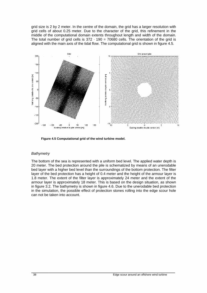
38 Edge scour around an offshore wind turbine
grid size is 2 by 2 meter. In the centre of the domain, the grid has a larger resolution with grid cells of about 0.25 meter. Due to the character of the grid, this refinement in the middle of the computational domain extents throughout length and width of the domain. The total number of grid cells is 372 · 190 = 70680 cells. The orientation of the grid is aligned with the main axis of the tidal flow. The computational grid is shown in figure 4.5.
Figure 4.5 Computational grid of the wind turbine model.
Bathymetry
The bottom of the sea is represented with a uniform bed level. The applied water depth is 20 meter. The bed protection around the pile is schematized by means of an unerodable bed layer with a higher bed level than the surroundings of the bottom protection. The filter layer of the bed protection has a height of 0.4 meter and the height of the armour layer is 1.8 meter. The extent of the filter layer is approximately 24 meter and the extent of the armour layer is approximately 18 meter. This is based on the design situation, as shown in figure 3.2. The bathymetry is shown in figure 4.6. Due to the unerodable bed protection in the simulation, the possible effect of protection stones rolling into the edge scour hole can not be taken into account.

Edge scour around an offshore wind turbine 39
Figure 4.6 Bathymetry around the pile.
Boundary conditions
Boundary conditions of the Riemann type are applied on the short boundaries of the domain. The long boundaries are closed. The weakly reflective Riemann boundaries are applied to prevent unintentional waves from being reflected back into the computational domain. The velocities are specified perpendicular to the short boundaries. Values for the velocity at the location of the most southern wind turbine in the large scale model described are applied on the short boundaries. No transport of sediment is simulated over the boundaries.
Wind turbine foundation
The support structure of the wind turbine is schematized with dry points, cells that are permanently dry during a computation. Eighteen dry points represent the diameter of the pile. Due to the nature of the grid, the wind turbine support structure consists of cells with a rectangular shape. This introduces stair case boundaries, which might cause artificial wall friction and flow separation.
4.3 Amplification factor
With the results of the Delft3D-Flow simulation, the amplification of the flow velocity downstream the wind turbine can be calculated. The amplification factor, called K-factor, is calculated by means of time series of the velocity at a location just downstream the bed protection. With this method is assumed that the K-factor is constant for different velocities. However, in reality, the Reynolds number, and thus the flow regime around the wind turbine foundation, changes with different velocities, see figure 2.2. In practice, this effect will be limited, as the velocity needs to be larger than the critical velocity in order to erode sediment. Even with a velocity of 0.1 meter per second, which is rather small for a critical velocity, a pile diameter of 4.6 meter and a kinematic viscosity of 10-6 meter2 per second, the Reynolds number is equal to 4.6·106 and the flow is still in the critical turbulence regime. This means that in any situation in which sediment is eroded, the

40 Edge scour around an offshore wind turbine
wake is completely turbulent. Dependence of the K-factor on the velocity is therefore not taken into account in this thesis. The transport of sediment has a non-linear relation with the velocity, larger velocities cause a considerable larger sediment transport. Taking the average amplification of the flow over a time series for the K-factor would cause an underestimation of the sediment transport. However, taking the maximum amplification of the flow, would cause the sediment transport to be overestimated, as this maximum velocity only occurs very rarely.
4.4 Edge scour prediction model
A model has been developed to calculate edge scour depth. This Edge Scour Prediction Model (ESPM) is based on mathematical relations of development towards an equilibrium in time and on empirical relations for the equilibrium edge scour depths and characteristic timescales. The Edge Scour Prediction Model assumes that the edge scour depth approaches an equilibrium depth for every occurring environmental condition, analogous to RAAIJMAKERS & RUDOLPH (2008) and RUDOLPH et al. (2008). According to these authors, local scour development in time can be described by an exponential function as equation 4.1.
1 expeqchar
tS t ST
4.1
in which S Edge scour depth [L] Seq Equilibrium edge scour depth [L] t Time [T] Tchar Characteristic time scale [T] The use of this formula implies that the scour depth approaches an equilibrium scour depth without completely reaching it. When the time is equal to the characteristic time scale Tchar, the scour depth is calculated to be 63 percent of the equilibrium scour depth Seq. It seems plausible that this is valid not only for local scour development, but for edge scour development as well, and that therefore equation 4.1 is also applicable for the edge scour depth as function of time. In this method, for every occurring combination of water depth and approach velocity in time series of 2006 to 2011, the equilibrium scour depth and the characteristic timescale are determined. These time series are predicted values, originating from an operational model. With these parameters and equation 4.1, the edge scour depth is calculated by means of a discretized formulation, shown in equation 4.2.
1 , 1 , 1 expn eq n n eq nchar
tS S S ST
4.2
This concept is illustrated in figure 4.7, where the first two graphs show the occurring flow velocity magnitude and the water depth, with which the equilibrium edge scour depth (third graph) and the characteristic time scale (fourth graph) are calculated. With the values in the third and fourth graph, the edge scour depth is calculated by means of equation 4.2.

Edge scour around an offshore wind turbine 41
Figure 4.7 Conceptual approach of the Edge Scour Prediction Model.
When the edge scour depth is smaller than the equilibrium edge scour depth at that moment, an increase of edge scour depth results. When the edge scour depth is larger than the equilibrium edge scour depth, backfilling takes place and the edge scour depth decreases. The characteristic timescale of backfilling is assumed to be equal to the characteristic timescale of edge scouring. Although local scour timescales of backfilling are easily about a factor ten larger than scouring timescales [RAAIJMAKERS & RUDOLPH (2008)], this seems to be a reasonable first assumption.
4.4.1 Equilibrium edge scour depth
One of the parameters to be defined in order to apply this model is the equilibrium depth. The equilibrium edge scour depth is calculated by means of a method that assumes that the effect of the velocity downstream of the wind turbine foundation is a factor K larger than the velocity upstream of the wind turbine foundation. This factor K accounts for additional velocity and turbulence and the resulting extra pick up of sediment due to the presence of the wind turbine. The bed load, suspended load and total load transport upstream of the pile are calculated with the sediment transport formulation of Van Rijn (1984), shown in equation 4.3, 4.4 and 4.5 respectively.
2.4 1.2
0 50,0 0 0
050
0.005 cb
U U ds U h
hgd 4.3
2.4
0.60 50,0 0 0 *
050
0.012 cs
U U ds U h D
hgd 4.4
,0 ,0 ,0s b sq s s 4.5

42 Edge scour around an offshore wind turbine
with:
1/3
* 50gD d 4.6
640 10
20 T 4.7
in which sb,0 Bed load sediment transport per unit width upstream [L2T-1] U0 Depth averaged velocity upstream [LT-1] h0 Water depth upstream [L] Uc Critical depth averaged velocity [LT-1]
Relative density [-] g Gravitational acceleration constant [LT-2] d50 Median grain diameter [L] ss,0 Suspended load sediment transport per unit width upstream [L2T-1] D* Sedimentological diameter [-] qs,0 Total sediment transport upstream [L2T-1] Kinematic viscosity [L2T-1]
T Temperature [°C] Downstream of the wind turbine, the factor K is applied. This results in equation 4.8, 4.9 and 4.10 for the bed load, suspended load en total load sediment transport downstream the wind turbine foundation respectively. However, also other sediment transport formulations could be easily implemented in this ESPM.
2.4 1.2
1 50,1 1 1
150
0.005 cb
KU U ds KU h
hgd 4.8
2.4
0.61 50,1 1 1 *
050
0.012 cs
KU U ds KU h D
hgd 4.9
,1 ,1 ,1s b sq s s 4.10 sb,1 Bed load sediment transport per unit width downstream [L2T-1] U1 Depth averaged velocity downstream [LT-1] h1 Water depth downstream [L] ss,1 Suspended load sediment transport per unit width downstream [L2T-1] qs,1 Total sediment transport downstream [L2T-1] K Coefficient depending on the flow velocity and turbulence
intensity [-]
In an equilibrium situation, the sediment transport upstream should be equal to the sediment transport downstream the wind turbine support structure. This means: ,0 ,1s sq q 4.11 The critical velocity is calculated with equation 4.12.
*,cc
D
UU
C 4.12
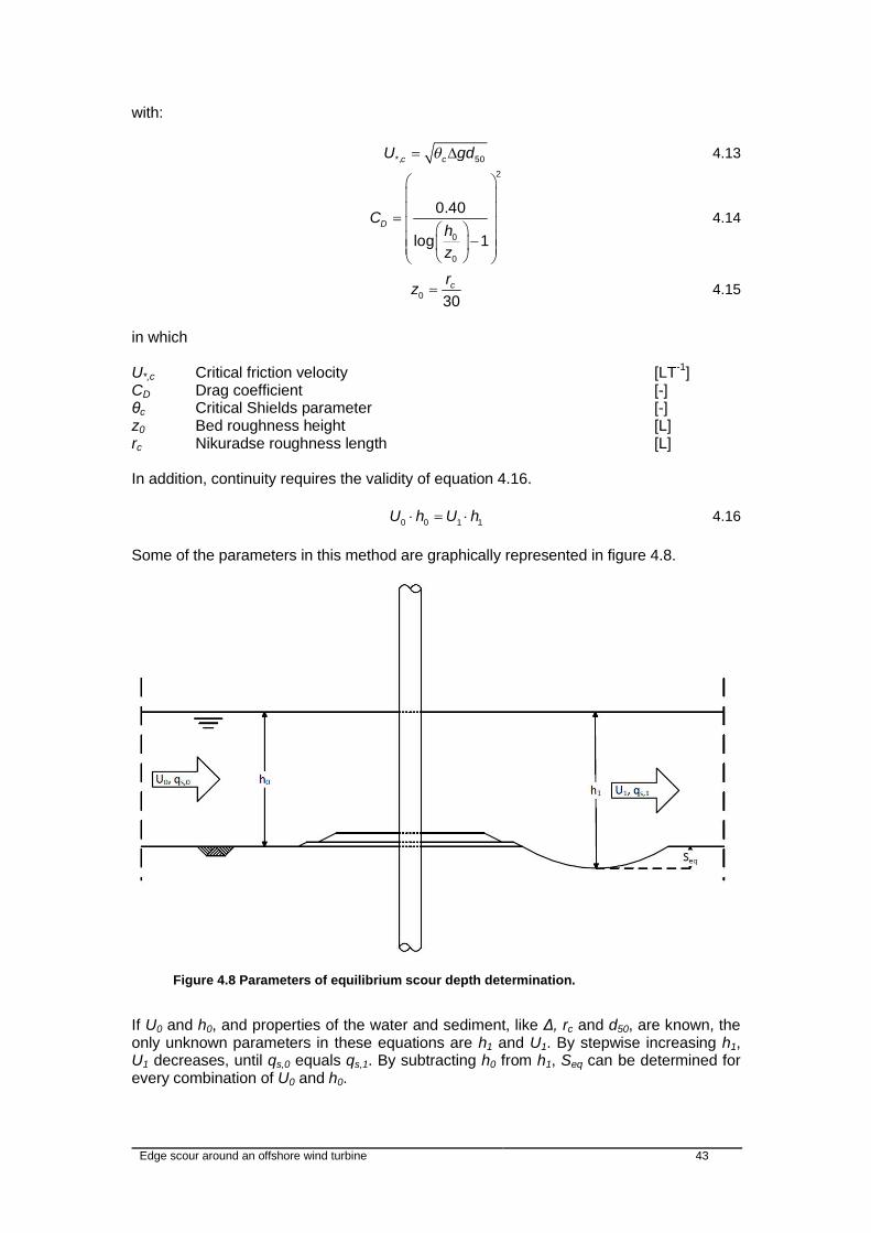
Edge scour around an offshore wind turbine 43
with: *, 50c cU gd 4.13
2
0
0
0.40
log 1DC
hz
4.14
0 30crz 4.15
in which U*,c Critical friction velocity [LT-1] CD Drag coefficient [-]
c Critical Shields parameter [-] z0 Bed roughness height [L] rc Nikuradse roughness length [L] In addition, continuity requires the validity of equation 4.16. 0 0 1 1U h U h 4.16 Some of the parameters in this method are graphically represented in figure 4.8.
Figure 4.8 Parameters of equilibrium scour depth determination.
If U0 and h0, and properties of the water and sediment, like , rc and d50, are known, the only unknown parameters in these equations are h1 and U1. By stepwise increasing h1, U1 decreases, until qs,0 equals qs,1. By subtracting h0 from h1, Seq can be determined for every combination of U0 and h0.

44 Edge scour around an offshore wind turbine
4.4.2 Characteristic timescale
For the characteristic timescale, an expression by Dietz (1969), mentioned by HOFFMANS & VERHEIJ (1997) for the characteristic time of scour downstream a bed protection of a sill is adapted. The expression by Dietz (1969) is written in equation 4.17.
1.5
04.0 2.5 0.5
0 Recharu
h CTu Fr
4.17
with
0
0
UFr
gh 4.18
0 0Re U h 4.19
0
cu
UK
U 4.20
in which Tchar Characteristic time scale [T] C Coefficient [-] Fr Froude number [-] Re Reynolds number [-] Kinematic viscosity [L2T-1] u Coefficient [-]
K Coefficient depending on the flow velocity and turbulence intensity
[-]
Dietz (1969) applied a value of 9.96·106 for the empirical coefficient C. The rate at which the scour hole approaches an equilibrium situation is highly sensitive to the turbulence intensity in non-uniform flow. Due to the presence of the wind turbine foundation and the vortex street behind it, the turbulence intensity is substantially larger compared to a situation with a sill only. As a consequence of this, the bed material is eroded faster. The timescale by Dietz (1969) is essentially applicable in situations where the equilibrium scour depth Seq downstream a sill is larger than the initial flow depth h0. However, in the case of edge scour around an offshore wind turbine, the equilibrium edge scour depth is smaller than the initial flow depth. Consequently, the process of approaching an equilibrium situation happens at a considerable higher rate, equivalent to a smaller timescale. The value for the coefficient C is therefore adapted and a value for C of 2·105 is used, a value approximately 50 times smaller than suggested by Dietz (1969).

Edge scour around an offshore wind turbine 45
5 Determination of amplification factor
The model of the area around a single wind turbine foundation has been run for one spring tidal cycle, starting with flow in the flood direction. Output has been generated every five minutes. In addition, a shorter simulation with output every six seconds has been run. This high frequent model output guarantees that the simulation of one lee-wake vortex is represented by multiple time steps in the output. In this simulation, a short period with the highest velocities of a spring tidal cycle is simulated. The results of the runs are presented in this chapter. In section 5.1 the hydrodynamic results of the simulations are presented, while section 5.2 presents the morphodynamic results. In the last section of this chapter, section 5.3, is the value for the K-factor determined.
5.1 Hydrodynamic results and analysis
The depth averaged velocity and the bed shear stress, both important for the sediment transport and bed level changes, are presented here. Section 5.1.1 demonstrates the depth averaged velocity and the bed shear stress is displayed in section 5.1.2.
5.1.1 Depth averaged velocity
The hydrodynamic results of the model simulations demonstrate the development of a vortex street behind the pile and flow contraction on both sides of the pile, as is shown in figure 5.1, which shows the instantaneous depth averaged velocity in part of the computational domain. The largest circle in this figure represents the extent of the filter layer of the bed protection, the smaller circle depicts the armour layer and the white circle represents the wind turbine support structure. The water flows from south to north and the undisturbed flow velocity equals approximately 0.75 meter per second.
Figure 5.1 Instantaneous depth averaged velocity.

46 Edge scour around an offshore wind turbine
In the results of model of the area around one wind turbine support structure, a distinct vortex street is developing in the flow downstream of the wind turbine support structure and the maximum depth averaged velocity and bed shear stress are situated on the north-north-east side of the wind turbine. Furthermore, the flow contraction on both sides of the wind turbine is well represented. The Reynolds number, expressed in equation 2.1, has a value in the order of 3·106. The Strouhal number, represented by equation 2.2, is in the simulation approximately equal to 0.17. This means, according to figure 5.2, that the frequency of the vortex shedding is reasonably well predicted by the model.
Figure 5.2 Variation of the Strouhal number with the Reynolds number and situation in OWEZ [SUMER & FREDSØE (1997)].
The mean and the maximum depth averaged velocity during one tidal cycle in time steps of five minutes is depicted in figure 5.3 for part of the computational domain.
Figure 5.3 Mean and maximum depth averaged velocity magnitude.
The highest velocities in the domain occur in two strips situated on the north side on the flanks of the pile. The velocity straight downstream the wind turbine foundation is in general lower than the velocity upstream the foundation of the wind turbine.

Edge scour around an offshore wind turbine 47
For a small period of fifteen minutes with a high frequent output, the mean and the maximum depth averaged velocities are normalized with the background depth averaged velocity. This background depth averaged velocity is the time-mean or time-maximum depth averaged velocity occurring 100 meter southwards of the wind turbine. During this period of fifteen minutes, the currents flow in north-north-east direction and output has been generated every six seconds. In this manner, the simulation of one vortex is represented by multiple time steps. The results are shown in figure 5.4.
Figure 5.4 Normalized mean and maximum depth averaged velocity magnitude.
5.1.2 Bed shear stress
The velocities over one tidal cycle give rise to mean and maximum bed shear stresses as displayed in figure 5.5.
Figure 5.5 Mean and maximum bed shear stress magnitude.

48 Edge scour around an offshore wind turbine
The bed shear stresses simulated in the short simulation with high frequent output are normalized by dividing the local bed shear stress by the background bed shear stress occurring 100 meter south of the wind turbine foundation. The resulting patterns are shown in figure 5.6.
Figure 5.6 Normalized mean and maximum bed shear stress magnitude.
The results representing the depth averaged velocity and the bed shear stress averaged or maximized over one tidal cycle demonstrate a rough pattern, especially the maximum values of the parameters. This is due to the relative low frequency of output over which is averaged or maximized. In the results of the simulations over a short period with high frequent output, the pattern is more smooth. Practical limitations prevent the processing of the results of a complete tidal cycle at a high frequency. However, the results over one tidal cycle give a good impression of the effect of the tidal asymmetry.
5.2 Morphodynamic results and analysis
Based on the hydrodynamic results, the morphological development is simulated. The next sections present the magnitude of the sediment transport around the support structure of the wind turbine and the resulting bed levels for different sediment transport formulations.
5.2.1 Sediment transport magnitude
With the sediment transport formulation of Van Rijn (1993), the sediment transport is calculated and averaged over fifteen minutes. In addition, the results are normalized by dividing the local bed shear stress by the background sediment transport magnitude occurring 100 meter south of the foundation of the wind turbine. The results for the middle part of the domain are shown in figure 5.7.
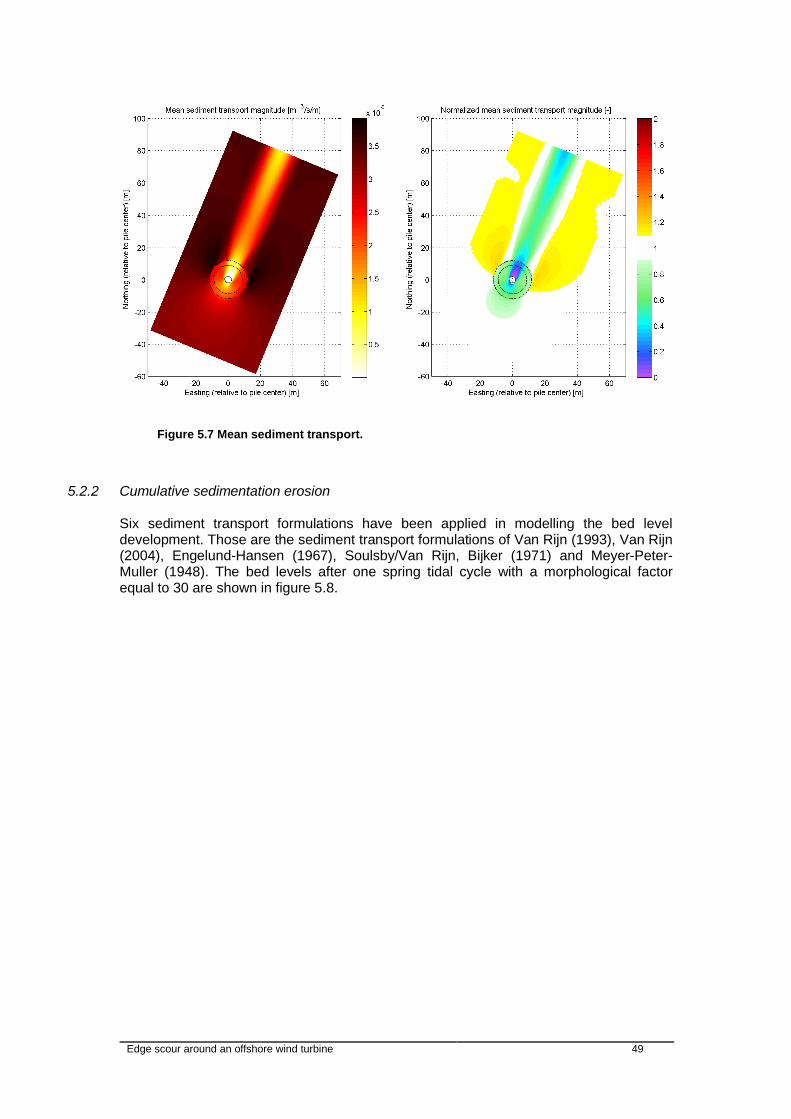
Edge scour around an offshore wind turbine 49
Figure 5.7 Mean sediment transport.
5.2.2 Cumulative sedimentation erosion
Six sediment transport formulations have been applied in modelling the bed level development. Those are the sediment transport formulations of Van Rijn (1993), Van Rijn (2004), Engelund-Hansen (1967), Soulsby/Van Rijn, Bijker (1971) and Meyer-Peter-Muller (1948). The bed levels after one spring tidal cycle with a morphological factor equal to 30 are shown in figure 5.8.

50 Edge scour around an offshore wind turbine
Figure 5.8 Cumulative sedimentation and erosion for different sediment transport formulations.
None of the resulting cumulative sedimentation and erosion patterns shown in figure 5.8 provides results that are similar to the measurements of the bed levels in OWEZ. Part of the reason for the lack of resemblance between the measurements and the model results is the atypical area of application in this research, being offshore, while the formulations are designed for application in coastal areas, estuaries and rivers. Especially the fact that straight downstream the wind turbine support structure in the bed level surveys edge scour is located, while the model predicts with all sediment transport formulations a certain degree of deposition at that location, is remarkable. Probably, this is due to the possibility that the hydrodynamics are not correctly simulated by the model. Presumably at least the maximum velocities straight downstream the wind turbine foundation are not simulated to be high enough at certain moments of time. This can have a number of reasons.
Firstly, it is noticeable that the flow particles with high velocities due to the flow contraction developing at one side of the wind turbine foundation, stay on the same side of the wind turbine foundation during their convection downstream. If these particles with high velocities are being drawn across the imaginary line from the centre of the wind turbine foundation downstream, the velocity straight downstream the wind turbine foundation is at certain moments higher than average.
Another possibility is that three-dimensional effects in the vortex street are responsible for higher velocity magnitudes straight downstream the wind turbine support structure. These effects cannot be modelled with this two dimensional model.
Due to the staircase boundary of the cylinder, the separation points of the vortices are at a fixed position at the widest point of the structure, see figure 5.9. However, the separation points of the vortices should move over the part of the

Edge scour around an offshore wind turbine 51
skin of the wind turbine foundation, as is visible in figure 5.10, where model results of a simulation with D-Flow FM are shown. This newly developed model was not available at the start of this research, but seems to generate promising results. In addition, the current at the boundaries is schematized to flow only perpendicular to the short boundaries and the interaction between the horseshoe vortex and the flow is not simulated. These facts could cause a lack of natural variability in the flow. In reality the flow could become more irregular, which could cause higher maximum velocities straight downstream the wind turbine support structure. This variability in flow velocity magnitudes is demonstrated by DARGAHI (1989) and Deltares, as is mentioned in section 2.1.2.
Which of these reasons is correct, can only be ascertained if detailed velocity measurements at a high resolution are available for calibration and validation of the model. With these velocity measurements, a conclusion can be drawn in terms of the flow pattern downstream a circular cylinder in current.
Figure 5.9 Separation points of vortices in Delft3D-Flow simulation at two times
Figure 5.10 Separation points of vortices in D-Flow FM at two times
Vorticity and turbulence intensity are important factors for the picking up sediment. These phenomena occur to a large extent in the vortices in the lee-wake of the foundation of the wind turbine, but are not taken into account in the sediment transport formulations in Delft3D or in any other existing sediment transport formulation.

52 Edge scour around an offshore wind turbine
Figure 5.8 shows large differences between the results with different sediment transport formulations. The formulation of Van Rijn (2004) gives very high and very low bed levels in grid cells adjacent to each other. This is not according to expectation. This formulation is most likely not correctly implemented in Delft3D-Flow. All other sediment transport formulations predict erosion at the transition of the bed protection and the sandy bed slightly to the sides of the wind turbine foundation. Straight downstream of the wind turbine foundation for the flood tide, all sediment transport formulations predict deposition of sediment to a certain degree. These locations of sedimentation and erosion correspond to the locations of the high and low flow velocities, as described in section 5.1. The formulations of Engelund-Hansen (1967), Bijker (1971) and Meyer-Peter-Muller (1948) reproduce results without an extensive strip of sedimentation straight behind the wind turbine foundation. These formulations are all formulations in which bed load transport plays a dominant role, either because the transport is imposed as bed load transport or because the suspended load transport is linearly dependent on the bed load transport. This is in contrast with the van Rijn formulations, which use separate formulations for bed load and suspended load transport. As particles transported by bed load transport generally travel less far than sediment in suspension, the influence of the wind turbine support structure on the morphological development is confined to the region close to the wind turbine for the formulations by Engelund-Hansen (1967), Bijker (1971) and Meyer-Peter-Muller (1948). This is an explanation for the differences between these and the other sediment transport formulations. During the ebb tide as well as during the flood tide, edge scour develops on either downstream side of the wind turbine support structure in the model simulation. During the ebb tidal currents, the edge scour hole that developed on the north-north-east side of the wind turbine foundation during the flood tide, becomes less deep. Backfilling takes place. It seems plausible that in this process an explanation can be found for the fact that in the bed level measurements of OWEZ, no edge scour can be discovered on the south-south-west side of the wind turbine foundation. As the tide is flood dominant, the higher velocities in flood direction can cause complete backfilling of the edge scour hole on the south-south-west side of the wind turbine foundation. The smaller velocities in ebb direction cause the edge scour hole on the north-north-east side of the wind turbine foundation to become less deep, but do not completely flatten out the edge scour hole on this side. The degree to which the tide is asymmetric is a very important factor in the development of edge scour. The deepest edge scour hole in the simulations occurs just outside the bed protection, on the transition between the bed protection and the erodable bed, while the measurements of the bed levels in OWEZ demonstrate that the deepest point is in reality slightly away from the bed protection. This can be explained by the fact that in reality the bed protection can degrade and stones can roll into the edge scour hole, armouring the slope of the hole. In the simulation, the bed protection is schematized by an unerodable bed. This causes a very steep slope just outside the bed protection on the transition between the bed protection and the sandy bed, which would not occur in reality. The hydrodynamic model is only calibrated with limited data. Caution is therefore required when interpreting the hydrodynamic results and the morphodynamic results, as they are based on the hydrodynamics.
5.3 Amplification factor
The depth averaged velocity magnitude in figure 5.4 suggests that the amplification of the flow velocity downstream the wind turbine foundation, just outside the bed protection, has a value between 1 and 1.3. The amplification of the bed shear stress just outside the bed

Edge scour around an offshore wind turbine 53
protection is approximately between 1.1 and 1.6, see figure figure 5.6. As the bed shear stress is a function of the velocity squared, the K-factor can be calculated by the square root of these factors. This would give a K-factor between 1.05 and 1.26. The measured values of the flow velocity around a circular cylinder by Deltares in section 2.1.2 give a K-factor between 0.76 and 1.96. The values for K simulated with Delft3D-Flow are within this range. The value for the K-factor should be larger than 1. Taking into account these considerations, a good value for the K-factor seems to be 1.2.


Edge scour around an offshore wind turbine 55
6 Edge scour depth
This chapter elaborates on the results of the Edge Scour Prediction Model. In the first two sections, the equilibrium edge scour depth and the characteristic timescale are discussed. In section 6.3 the calculated edge scour depth is compared with values for the edge scour depth measured in OWEZ. The tidal asymmetry in OWEZ is subject of section 6.4 and in section 6.5 is the influence of several parameters is investigated. Finally, the last section of this chapter elaborates on possible practical applications of the ESPM.
6.1 Equilibrium edge scour depth
Results for the ESPM are generated for approach velocities between 0 and 1.4 meter per second with water depths between 16 and 21 meter. A K-factor of 1.2 is applied. The equilibrium edge scour depth and the characteristic timescales for this range of values is shown in figure 6.1.
Figure 6.1 Equilibrium edge scour depth.

56 Edge scour around an offshore wind turbine
Figure 6.1 demonstrates that the equilibrium edge scour depth hardly has a relation to the approach flow velocity and is almost linearly dependent on the water depth. The weak dependence on the approach flow velocity is supported by MELVILLE & COLEMAN (2000), who describe this effect for the local scour depth. They state that the live-bed scour depth, for velocities larger than the threshold velocity, is largely independent of flow velocity. Also, the authors who relate the scour depth to the pile diameter in section 2.2, do not describe any dependency on the flow velocity for current-only situations. An almost linear dependence of the equilibrium edge scour depth on the water depth is predicted by Dietz (1960) in HOFFMANS & VERHEIJ (1997) and in equation 2.10 and equation 2.11.
6.2 Characteristic timescale
For the same range of conditions as for the equilibrium edge scour depth, the characteristic timescale is determined and shown in figure 6.2.
Figure 6.2 Characteristic timescale.
The characteristic timescale has a weak inversely proportional relation with the water depth and a strong relation with the approach flow velocity in this method. This is according to expectation, as a low velocity erodes only a small amount of sediment. This causes the characteristic timescale to be large for a low flow velocity.
6.3 Comparison with measured edge scour depth
The time series of flow velocities and water levels provide the opportunity to determine the equilibrium edge scour depth and the characteristic timescale for all occurring

Edge scour around an offshore wind turbine 57
conditions of the velocities and water depths, by interpolation of figure 6.1 and figure 6.2. With these parameters and equation 4.2, the edge scour development in time can be calculated. The result is shown in figure 6.3. The measured edge scour depths at all piles are plotted in the figure as well.
Figure 6.3 Edge scour depth with Edge Scour Prediction Model and measured values for edge scour depth.
The estimated edge scour depth agrees reasonably well with the measured values of the edge scour depth, especially for the three wind turbine foundations shown in figure 6.4.
Figure 6.4 Predicted edge scour depth and measured edge scour depth for three individual wind turbine foundations
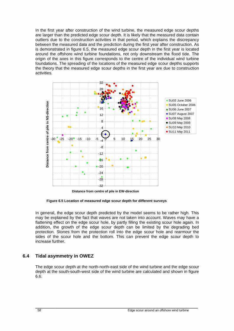
58 Edge scour around an offshore wind turbine
In the first year after construction of the wind turbine, the measured edge scour depths are larger than the predicted edge scour depth. It is likely that the measured data contain outliers due to the construction activities in that period, which explains the discrepancy between the measured data and the prediction during the first year after construction. As is demonstrated in figure 6.5, the measured edge scour depth in the first year is located around the offshore wind turbine foundations, not only downstream the flood tide. The origin of the axes in this figure corresponds to the centre of the individual wind turbine foundations. The spreading of the locations of the measured edge scour depths supports the theory that the measured edge scour depths in the first year are due to construction activities.
-32
-28
-24
-20
-16
-12
-8
-4
0
4
8
12
16
20
24
28
32
-30 -25 -20 -15 -10 -5 0 5 10 15 20 25 30
Distance from centre of pile in EW-direction
Dis
tanc
e fr
om c
entr
e of
pile
in N
S-di
rect
ion SU02 June 2006
SU05 October 2006SU06 June 2007SU07 August 2007SU08 May 2008SU09 May 2009SU10 May 2010SU11 May 2011
Figure 6.5 Location of measured edge scour depth for different surveys
In general, the edge scour depth predicted by the model seems to be rather high. This may be explained by the fact that waves are not taken into account. Waves may have a flattening effect on the edge scour hole, by partly filling the existing scour hole again. In addition, the growth of the edge scour depth can be limited by the degrading bed protection. Stones from the protection roll into the edge scour hole and rearmour the sides of the scour hole and the bottom. This can prevent the edge scour depth to increase further.
6.4 Tidal asymmetry in OWEZ
The edge scour depth at the north-north-east side of the wind turbine and the edge scour depth at the south-south-west side of the wind turbine are calculated and shown in figure 6.6.

Edge scour around an offshore wind turbine 59
Figure 6.6 Edge scour depth at the north-north-east and south-south-west side of the wind turbine.
A distinct difference between the edge scour depth on the north-north-east side of the wind turbine and the south-south-west side of the wind turbine is visible in figure 6.6. This is in agreement with the effect of the tidal asymmetry, described in section 5.2. However, the edge scour depth on the south-south-west side of the wind turbine, is not zero or very close to zero. This might also be attributed to the lack of the flattening effect of waves in the Edge Scour Prediction Model.
6.5 Influence of parameters
The dependency of edge scour on the tidal asymmetry, on the amplification factor and on the median sediment diameter is further investigated. To rule out other effects than the ones investigated, an artificial tidal signal is created with S2 and M2 tidal components. The maximum spring velocity is equal to 0.78 meter per second, while the maximum neap velocity is equal to 0.4 meter per second, unless stated otherwise.
6.5.1 Tidal asymmetry
For a completely symmetric tide, edge scour develops on both sides of the wind turbine foundation with the same rate, as is shown in figure 6.7. In this figure, both lines are on top of each other. Although the tide is symmetric, the ESPM predicts the development of edge scour on both sides of the wind turbine foundation. This is due to the fact that the backfilling process goes slower than the erosion in the ESPM in the early stages of the development of edge scour. This is because during the backfilling, the equilibrium edge scour depth is equal to zero, while it has a certain value during the process of erosion. Although the characteristic time scales in the ESPM are assumed to be equal during backfilling and erosion, the process of backfilling is slower during the beginning of edge scour development, as the difference between the actual edge scour depth and the equilibrium edge scour depth during backfilling is smaller than the difference between the actual

60 Edge scour around an offshore wind turbine
edge scour depth and the equilibrium edge scour depth during erosion. The expression for the development of edge scour is dependent on this difference, see equation 4.2.
Figure 6.7 Edge scour development in time for a symmetric tide.
The relation between edge scour depth and the asymmetry factor, defined as the ratio of the flood velocities and the ebb velocities, is plotted in figure 6.8. The larger the asymmetry factor, the larger the edge scour depth on the downstream side of the structure for the dominant tide.
Figure 6.8 Relation between edge scour and asymmetry factor.

Edge scour around an offshore wind turbine 61
Not only the tidal asymmetry is important for edge scour development, the absolute tidal velocities play a significant role as well. The edge scour after five years for different maximum spring velocities and a number of asymmetry factors is shown in figure 6.9.
Figure 6.9 Relation between edge scour and maximum spring velocity and tidal asymmetry
6.5.2 Amplification factor
The effect of the amplification factor in the ESPM on the prediction of the development of edge scour is considerable as demonstrated for a symmetric tide in figure 6.10.
Figure 6.10 Relation between edge scour and K-factor for a symmetric tide.

62 Edge scour around an offshore wind turbine
For the tide in OWEZ, the effect of the K-factor on the development of edge scour is demonstrated in figure 6.11.
Figure 6.11 Edge scour depth for the tide in OWEZ with several K-factors.
As can be expected, for a K-factor of one, no edge scour takes place, as no amplification of the flow is taken into account. The non-linear effect of the K-factor is clearly visible in figure 6.11.
6.5.3 Median sediment diameter
The influence of the median sediment diameter is depicted in figure 6.12, where the edge scour development for a symmetric tide is shown for different sediment diameters. A smaller sediment diameter results in a larger edge scour depth. This is according expectation, as smaller particles are more prone to erosion than larger particles.

Edge scour around an offshore wind turbine 63
Figure 6.12 Edge scour depth for a symmetric tide with different median sediment diameters
6.6 Prediction of edge scour depth for OWEZ
Under the assumption that the same hydrodynamic conditions as in the last years occur in the coming years, a prediction of the edge scour depth can be made for the future. According to the ESPM, an equilibrium situation arises after approximately 10 years. The edge scour depth on the north side of the wind turbine support structure is then about 2.9 meter. On the south side, the edge scour depth is than approximately 0.8 meter. The predicted edge scour development in time is shown in figure 6.13.
Figure 6.13 Prediction of edge scour development

64 Edge scour around an offshore wind turbine
6.7 Practical application of the ESPM
The results for this specific situation look promising, but the ESPM is also easily applicable to other environmental situations or for other bed protections. If for another situation time series of velocities are available and the K-factor is determined, an first estimation of the edge scour is easily made with the ESPM. If a good numerical model for flow around a wind turbine support structure becomes available, it is well likely that it has a large run time. With the ESPM, it is only needed to run a short time simulation with the numerical model, including the shedding of a number of vortices. From that short simulation, the K-factor can be determined and with time series of the velocity, a first estimate of the edge scour depth can be obtained and used in a new design of bed protection. Edge scour development near bed protections with another shape can be assessed with the ESPM as well. The results of the simulations in chapter 5 suggest that the amplification of the flow decreases with increasing distance of the wind turbine foundation. Therefore, less edge scour is to be expected at larger distance from the wind turbine support structure. This can be used to assess other shapes of bottom protection, for example egg shaped, like demonstrated in figure 6.14. With the same amount of stones, and therefore approximately the same costs, as currently in OWEZ, but less stones on the sides and more stones on the north side of the wind turbine, less edge scour is supposed to occur. Moreover, the edge scour occurs further downstream of the wind turbine support structure.
Figure 6.14 Egg shaped bottom protection around wind turbine support structure.
This is supported by the bed level measurements around wind turbine 10 in OWEZ. The abnormal construction of the filter layer around this wind turbine support structure was already discussed in section 3.3.3. Around this wind turbine, the filter layer was originally placed slightly north east of the planned location, see figure 6.15. Later on, additional filter material has been placed to correct for this. For comparison, also the bed level development around the adjacent wind turbine is shown.

Edge scour around an offshore wind turbine 65
Figure 6.15 Bed level development around wind turbine 9 and 10 in OWEZ.
It is clearly visible that after five years, the edge scour depth around wind turbine 10 is located further downstream of the wind turbine compared with the edge scour depth around wind turbine with number 9. In addition, the edge scour depth around wind turbine 10 is shallower than the edge scour depth around wind turbine 9. A first estimate of the edge scour depth near a bed protection with another shape than egg-shaped requires a value for the K-factor at the edge of the other bed protection. For a financial assessment of different shape of bed protection in a design, the costs of the required amount of stones need to be balanced against the costs of the burial depth and location of cables.
Wind turbine 9 in 2006 Wind turbine 10 in 2006
Wind turbine 10 in 2011 Wind turbine 9 in 2011


Edge scour around an offshore wind turbine 67
7 Conclusions and recommendations
The development of edge scour around an offshore wind turbine is a complicated process, due to the complex flow field around a circular cylinder in current, especially downstream of the wind turbine. The flow field and the development of edge scour around an offshore wind turbine have been investigated and the Edge Scour Prediction Model has been developed in this research. This chapter elaborates on the results of this research in relation to the objectives. Section 7.1 describes the conclusions of this research. These conclusions lead to recommendations for further research given in section 7.2.
7.1 Conclusions
The following objectives were studied in this thesis: 1. Gain insight in the hydrodynamic and morphodynamic processes around the
foundation of an offshore wind turbine with bottom protection, focussing on edge scour.
2. Explore the possibilities of applying Delft3D-Flow for modelling the hydrodynamic and morphodynamic processes around the foundation of an offshore wind turbine with bottom protection, focussing on edge scour.
3. Develop a model to predict the depth and rate of edge scour around the foundation of an offshore wind turbine.
The first objective was to gain insight in the hydrodynamic and morphodynamic processes around the foundation of an offshore wind turbine with bottom protection, focussing on edge scour. With respect to this objective, the following conclusions can be drawn:
The asymmetry of the tide is of major concern in the development of edge scour. Edge scour develops mainly downstream the wind turbine for the dominant tide.
Lee-wake vortices downstream the wind turbine play an important role in the formation of the edge scour holes.
No clear relation between the height or volume of the bottom protection and the edge scour depth could be established. A longer filter layer seems to reduce the edge scour depth effectively
The exploration of the possibilities of applying Delft3D-Flow for modelling the hydrodynamic and morphodynamic processes around the foundation of an offshore wind turbine with bottom protection, focussing on edge scour, was the second objective. This objective leads to the following conclusions:
A lack of resemblance between the bed levels modelled with Delft3D-Flow and the measured bed levels in OWEZ exists. Straight north-north-east of the wind turbine is deposition of sediment predicted by Delft3D-Flow, while the measurements show erosion at that location. Most likely this is due to poor performance of the two dimensional model with respect to the hydrodynamics in this specific situation.

68 Edge scour around an offshore wind turbine
Hardly any data for validation of the flow field exist, which makes the judgement about the exact performance of the model with respect to the hydrodynamics a challenging task. The hydrodynamic results, and with those the morphodynamic results, should therefore be treated with caution.
The frequency of the vortex shedding can be estimated reasonably well by Delft3D-Flow.
The simulated bed level development is fairly sensitive to the sediment transport formulation used.
Regarding the third objective, being to develop a model to predict the depth and rate of edge scour around the foundation of an offshore wind turbine, the following conclusions can be drawn:
The Edge Scour Prediction Model, a model based on mathematical relations of development towards an equilibrium in time and empirical relations for the equilibrium edge scour depth and characteristic timescale, has proven to reproduce the edge scour depth as function of time in OWEZ reasonably well.
The ESPM can be a valuable tool for a first impression of the edge scour depth in new designs at other locations.
According to the ESPM, the edge scour in OWEZ reaches an equilibrium situation after approximately 10 years. The edge scour depth on the north side of the wind turbine is then 2.9 meter.
7.2 Recommendations
In order to obtain a better understanding of the flow field around an offshore wind turbine, the development of edge scour and modelling of edge scour around an offshore wind turbine, more research is required. The following aspects deserve attention in further research on these subjects.
7.2.1 Validation
In the present study, the hydrodynamic model results hardly have been validated, due to the lack of suitable validation data. In order to obtain validation data, the execution of laboratory experiments with flow around a circular cylinder is recommended. Velocity measurements on a high resolution around the cylinder, especially downstream in the developing vortex street, could result in more information about the flow patterns that are causing edge scour. With these measurements, the models could be properly validated.
7.2.2 Application of a numerical model
The current study shows that improvement of the numerical simulation in Delft3D is needed. A number of methods is recommended. Firstly, research on numerical modelling in three dimensions or with the non-hydrostatic version of Delft3D-Flow is recommended, if the drawbacks reported in section 4.2.1 could be overcome. The application of a flexible, or unstructured, mesh is recommended as well. The newly developed software package D-Flow FM could come in useful.
7.2.3 Schematization of the bottom protection
The schematization of the bed protection around the offshore wind turbine is in the current research a highly simplified representation of reality. Due to the fact that the bed protection is schematized to be unerodable is degradation of the bed protection not possible in the Delft3D-Flow model. However, degradation of the bed protection can be

Edge scour around an offshore wind turbine 69
expected in reality and the stones of the filter layer of the bed protection are able to roll in to the edge scour hole. This falling apron effect and its simulation in a numerical model is recommended to be subject of further research.
7.2.4 Edge scour prediction model
The present research has shown the large potential of a simple Edge Scour Prediction Model. However, more research is recommended to improve this method. The application of a well calibrated and validated numerical model could come in useful to determine the amplification of the flow velocity downstream the wind turbine and the bed protection. At this moment, the effect of waves is not incorporated in the ESPM. Also, the effect of the application of other sediment transport formulations or other formulations for the equilibrium scour depth and the characteristic timescale is recommended as a subject for further investigation.


Edge scour around an offshore wind turbine 71
8 References
BOSBOOM, J. & STIVE, M. J. F. (2011). Coastal Dynamics I, Lecture notes of CT4305 Delft University of Technology
CHIEW, Y.-M. (1995). Mechanics of Riprap Failure at Bridge Piers. Journal of Hydraulic Engineering, 121(9), 635-643.
DARGAHI, B. (1989). The tubulent flow field around a circular cylinder. Experiments in Fluids, 8, 1-12.
DE VOS, L. (2008). Optimisation of scour protection design for monopiles and quantification of wave run-up - Engineering the influence of an offshore wind turbine on local flow conditions. Ghent University, Ghent.
DELTARES. (2010). Delft3D-Flow User Manual. DEN BOON, J. H., SUTHERLAND, J., WHITEHOUSE, R., SOULSBY, R., STAM, C. J. M., VERHOEVEN,
K. et al. (2004). Scour Behaviour and Scour Protection for Monopile Foundations of Offshore Wind Turbines. Paper presented at the European Wind Energy Conference.
EWEA. (2011a). Wind energy and EU climate policy. Brussels. EWEA. (2011b). Wind in our Sails - The coming of Europe’s offshore wind energy industry.
Brussels. HOFFMANS, G. J. C. M. & PILARCZYK, K. W. (1995). Local Scour Downstream of Hydraulic
Structures. Journal of Hydraulic Engineering, 121(4), 326-340. HOFFMANS, G. J. C. M. & VERHEIJ, H. J. (1997). Scour manual. Rotterdam: Balkema. LESSER, G. R., ROELVINK, J. A., VAN KESTER, J. A. T. M. & STELLING, G. S. (2004). Development
and validation of a three-dimensional morphological model. Coastal Engineering, 51(8-9), 883-915.
LOUWERSHEIMER, W. F. (2007). Scour around an offshore wind turbine. Delft University of Technology, Delft.
MELVILLE, B. W. & COLEMAN, S. E. (2000). Bridge scour. Highlands Ranch, Colorado, USA: Water Resources Publications, LLC.
NIELSEN, A. W. & HANSEN, E. A. (2007). Time-varying wave and current induced scour around offshore wind turbines. Paper presented at the 26th International Conference on Offshore Mechanics and Arctic Engineering OMAE2007, San Diego, California, USA.
NIELSEN, A. W., SUMER, B. M., FREDSOE, J. & CHRISTENSEN, E. D. (2010). Scour protection around offshore wind turbines. Monopiles. Paper presented at the International Conference on Scour and Erosion, San Fransisco.
NOORDZEEWIND. (2011). www.noordzeewind.nl. Retrieved 03 januari 2012, 2011 RAAIJMAKERS, T. C., OEVEREN, M. C. V., RUDOLPH, D., LEENDERS, V. & SINJOU, W. C. P. (2010).
Field performance of scour protection around offshore monopiles. Paper presented at the Fifth International conference on scour and erosion, San Francisco, USA.
RAAIJMAKERS, T. C. & RUDOLPH, D. (2008). Time-dependent scour development under combined current and waves conditions - laboratory experiments with online monitoring technique. Paper presented at the Fourth International Conference on Scour and Erosion, Tokyo, Japan.
RAAIJMAKERS, T. C., RUDOLPH, D., VAN BERGEN, M. R. J. & VAN LIESHOUT, G. (2007). Offshore Windpark Egmond aan Zee – performance of scour protection and edge scour protection. Paper presented at the European Offshore Wind Conference, Berlin.
ROULUND, A., SUMER, B. M., FREDSOE, J. & MICHELSEN, J. (2005). Numerical and experimental investigation of flow and scour around a circular pile. Journal of Fluid Mechanics, 534, 351-401.
RUDOLPH, D. & BOS, K. J. (2006). Scour around a monopile under combined wavecurrent conditions and low KC-numbers. Paper presented at the Third International Conference on Scour and Erosion, Amsterdam.

72 Edge scour around an offshore wind turbine
RUDOLPH, D., RAAIJMAKERS, T. C. & STAM, C. J. M. (2008). Time-dependent scour development under combined current and wave conditions -hindcast of field measurements. Paper presented at the Fourth International Conference on Scour and Erosion, Tokyo, Japan.
SCHIERECK, G. J. (2004). Introduction to bed, bank and shore protection. Delft: Delft University Press.
SUMER, B. M. & FREDSØE, J. (1997). Hydrodynamics around cylindrical structures. Singapore: World Scientific.
SUMER, B. M. & FREDSØE, J. (2001). Scour around Pile in Combined Waves and Current. Journal of Hydraulic Engineering, 127(5), 403-411.
SUMER, B. M. & FREDSØE, J. (2002). The mechanics of scour in the marine environment. Singapore: World Scientific.
SUMER, B. M., HATIPOGLU, F. & FREDSØE, J. (2007). Wave Scour around a Pile in Sand, Medium Dense, and Dense Silt. Journal of Waterway, Port, Coastal, and Ocean Engineering.
UIJTTEWAAL, W. (2011). Turbulence in hydraulics, Lecture notes of CT5312 Delft University of Technology
UITTENBOGAARD, R. E. & VAN VOSSEN, B. (Eds.). (2003). Subgrid-scale model for Quasi-2D turbulence in shallow water. London: Taylor and Francis Group.
VAN DER TEMPEL, J. (2006). Design of support structures for offshore wind turbines. Technische universiteit Delft, Delft.
VAN VOSSEN, B. (2000). Horizontal large eddy simulations: evaluation of flow computations with Delft3D-flow. Delft University of Technology, Delft.
WHITEHOUSE, R. J. S., HARRIS, J. M., SUTHERLAND, J. & REES, J. (2011). The nature of scour development and scour protection at offshore windfarm foundations. Marine Pollution Bulletin, 62(1), 73-88.
ZHAO, M., CHENG, L. & ZANG, Z. (2010). Experimental and numerical investigation of local scour around a submerged vertical circular cylinder in steady currents. Coastal Engineering, 57(8), 709-721.

Edge scour around an offshore wind turbine 73
9 Appendix
The software used in this research is Delft3D. The hydrodynamic and transport module of Delft3D, Delft3D-Flow, is a simulation program for calculating non-steady flow and transport phenomena. A number of principles on which the Delft3D-Flow module is based will be discussed in more detail in this section. The content of this section is partly based on LESSER et al. (2004) and DELTARES (2010).
9.1 Basic equations
Delft3D-Flow solves the non-linear shallow water equations, derived from the Navier-Stokes equations for an incompressible fluid. Equation 9.1 shows the horizontal momentum equations as they are solved by Delft3D-Flow in a Cartesian coordinate system.
2
0
20
1 1
1 1
x x x V
y y y V
u u u u uu v fv P F Mt x y h hv v v v yu v fu P F Mt x y h h
9.1
in which u Velocity in x-direction [LT-1] v Velocity in y-direction [LT-1] t Time [T] h Water depth [L]
Vertical velocity component in sigma coordinate system [T-1] Vertical sigma coordinate [-]
f Coriolis coefficient [T-1] 0 Reference density of water [ML-3]
Pi Horizontal pressure in i-direction [ML-2 T-2] Fi Horizontal Reynolds stresses in i-direction [LT-2] Mi Contributions due to external sources of sinks of momentum in i-
direction [LT-2]
v Vertical kinematic viscosity coefficient [L2T-1] The horizontal Reynolds stresses are determined with equation 9.2.
2 2
2 2
2 2
2 2
x H
y H
u uFx y
v vFx y
9.2
in which
H Horizontal kinematic viscosity coefficient [L2T-1]

74 Edge scour around an offshore wind turbine
Under the shallow water assumption, the vertical momentum equation reduces to the hydrostatic pressure equation, given by equation 9.3.
P gh 9.3
in which P Pressure [ML-1 T-2]
Density of water [ML-3] g Gravitational acceleration constant [LT-2] The depth-averaged continuity equation is shown in equation 9.4.
hu hv
St x y
9.4
in which Water surface elevation above reference datum [L] Average velocity in x-direction [LT-1] v Average velocity in y-direction [LT-1]
S Contribution per unit area due to the discharge or withdrawal of water, evaporation and precipitation
[LT-1]
The transport equation, or advection-diffusion equation, is given in equation 9.5.
1
H H V
hc huc hvc ct x y
c c ch D D D hSx x y y h
9.5
in which c Mass sediment concentration [ML-3] DH Horizontal diffusion coefficient [L2T-1] DV Vertical diffusion coefficient [L2T-1] S Contribution per unit area due sources and sinks [ML-2T-1] In Delft3D-Flow, the horizontal viscosity and diffusivity are assumed to consist of three parts, namely the molecular viscosity, which is a constant value for a fluid, ‘3D turbulence’ and ‘2D turbulence’.
9.2 Turbulence closure models
In a 3D simulation In Delft3D-Flow, the vertical distribution of turbulence is calculated by a turbulence closure model. Four turbulence closure models are available in Delft3D-Flow: the constant, algebraic, k-L, and k- turbulence model. For the constant turbulence model, background values for the eddy viscosity and diffusivity are user specified. The other turbulent closure models implemented in Delft3D-Flow are based on the ‘eddy viscosity’ concept. The diffusion and viscosity coefficients are assumed to be proportional

Edge scour around an offshore wind turbine 75
to a length scale and a velocity scale and the four models differ in their prescription of the turbulent kinetic energy, the dissipation of energy and/or the mixing length.
9.3 Horizontal large eddy simulation
The horizontal distribution of turbulence is a measure of the horizontal mixing that is not resolved by advection on the horizontal computational grid. The values for this ‘2D turbulence’ can be user-defined, as a constant or varying in space, or can be computed by a sub-grid model for horizontal large eddy simulation (HLES). With this last method, large scale horizontal turbulent motions are computed, whereas the horizontal turbulent motions smaller than a certain length scale remain computationally unresolved and are modelled by a turbulence closure model. This method can be justified by the fact that the large scale horizontal turbulent motions are more energetic than the turbulent motions with smaller scales and the fact that they determine the general behaviour of the flow. Also, the large scale motion is strongly anisotropic, in contrast to the small scale motion. The most important function of the turbulence on the small scale is to withdraw energy from the large scale motions. [VAN VOSSEN (2000), UITTENBOGAARD & VAN VOSSEN (2003), UIJTTEWAAL (2011)]
9.4 Sediment transport and morphology
With the results of the hydrodynamic computations, Delft3D-Flow can simulate the sediment transport. At each computational time step, the change in mass of bed material is calculated, and based on that information, the bed level is updated. With the feedback of the bed level changes to the hydrodynamic computation, a full morphodynamic computation is executed. A number of sediment transport formulations are available in Delft3D, including Van Rijn (1993), Van Rijn (2004), Engelund-Hansen (1967), Soulsby/Van Rijn, Bijker (1971) and Meyer-Peter-Muller (1948). For the mathematic expressions of the formulas is referred to DELTARES (2010). In the formulations of Van Rijn (1993), Van Rijn (2004) and Soulsby/Van Rijn the sediment transport formulations are splitted in separate expressions for bed load transport and suspended load transport. This is in contrast to the formulations of Engelund-Hansen (1967) and Meyer-Peter-Muller (1948), in which the transport rate is imposed as bed load transport due to currents. The formulation by Meyer-Peter-Muller (1948) is similar to the Engelund-Hansen formulation. Both are total transport formulations, but the formulation of Meyer-Peter-Muller (1948) takes a critical bed shear stress into account, which makes it more advanced than the Engelund-Hansen formulation. Bijker (1971) derived a formulation for bed load transport in which the total load is expressed as the sum of a bed load transport and a suspended load transport. The suspended load transport is defined as function of the bed load transport.
9.5 Morphological acceleration factor
In many situations in coastal engineering, morphological changes take place on a considerable longer timescale than changes in the hydrodynamics. In order to reduce computation time in modelling this kind of situations, a morphological acceleration factor (morfac) is applied. In this method, the erosion and deposition fluxes from the bed to the flow and vice versa are multiplied with this morfac every computational time step. After simulating a certain hydrodynamic time span, the morphologic time span simulated is effectively morfac times as large. By doing so, is implicitly assumed that the bed level changes after one time step do not have a significant influence on the hydrodynamics. In addition, by following this approach, the order of the events is changed and should therefore not have a major influence.

76 Edge scour around an offshore wind turbine
9.6 Assumptions underlying Delft3D-Flow
Due to practical limitations, a number of assumptions are adopted in Delft3D-Flow, of which the most important ones for this research are listed below.
As mentioned before, Delft3D-Flow solves the non-linear shallow water equations. These equations are derived from the Navier-Stokes equations under the assumption of shallowness of the water. This means that the vertical length scales are assumed considerably smaller than the horizontal length scales. Accelerations in vertical direction are expected to be small compared to the gravitational acceleration. This might not be the case near the wind turbine foundation, but it is assumed that downstream the bed protection, at the location of the edge scour, this assumption is valid. Above the bed protection, no relevant morphological changes are expected to occur.
The flow is assumed to be incompressible in Delft3D-Flow. In order to calculate the bed shear stress, Delft3D-Flow takes into account only
the horizontal component of the velocity, assuming that the vertical component of the flow velocity is negligible.