edge/cloud virtualization techniques and resource
TRANSCRIPT
Alma Mater Studiorum
University of Bologna
SCHOOL OF SCIENCE
MASTER’S DEGREE IN COMPUTER SCIENCE
EDGE/CLOUD VIRTUALIZATION
TECHNIQUES AND RESOURCE
ALLOCATION ALGORITHMS
FOR IOT-BASED SMART
ENERGY APPLICATIONS
Supervisor:Prof.MARCO DI FELICE
Co-Supervisor:Prof.ANDREAS KASSLER
Author:VIVIANA RAFFA
III SessionAcademic Year 2019/2020


Abstract
Nowadays, the installation of residential battery energy storages (BES) has
increased as a consequence of the decrease in the cost of batteries. The cou-
pling of small-scale energy generation (residential PV) and residential BES
promotes the integration of microgrids (MG), i.e., clusters of local energy
sources, energy storages, and customers which are represented as a single
controllable entity. The operations between multiple grid-connected MGs
and the distribution network can be coordinated by controlling the power
exchange; however, in order to achieve this level of coordination, a control
and communication MG interface should be developed as an add-on DMS
(Distribution Management System) functionality to integrate the MG energy
scheduling with the network optimal power flow.
This thesis proposes an edge-cloud architecture that is able to integrate
the microgrid energy scheduling method with the grid constrained power
flow, as well as providing tools for controlling and monitoring edge devices.
As a specific case study, we consider the problem of determining the energy
scheduling (amount extracted/stored from/in batteries) for each prosumer
in a microgrid with a certain global objective (e.g. to make as few energy
exchanges as possible with the main grid).
The results show that, in order to have a better optimization of the BES
scheduling, it is necessary to evaluate the composition of a microgrid in such
a way as to have balanced deficits and surpluses, which can be performed
with Machine Learning (ML) techniques based on past production and con-
sumption data for each prosumer.
i

Keywords
Battery Energy Storage, Edge-cloud computing, Energy management sys-
tem, Energy scheduling, Energy sources, Energy trading, Internet of Things,
Message broker, Photovoltaic, Renewable Energy Source, Smart energy, Smart
grid, Time series.
ii
Sommario
Oggigiorno, in seguito alla diminuzione del costo delle batterie, l’installazione
di accumulatori di energia (BES) residenziali e aumentata. La combinazione
tra produzione di energia su piccola scala (PV residenziale) e BES residenziali
promuove lo sviluppo delle microgrids, cioe cluster di fonti locali, accumula-
tori e consumatori di energia rappresentati come una singola entita control-
labile. Le operazioni tra piu MG connesse alla rete e la rete di distribuzione
principale possono essere coordinate controllando lo scambio di energia, ma
per raggiungere questo livello di coordinamento, dovrebbe essere sviluppata
un’interfaccia MG di controllo e comunicazione come funzionalita DMS (Dis-
tribution Management System) aggiuntiva per integrare la programmazione
energetica della microgrid con il flusso ottimale della rete.
Questa tesi propone un’architettura edge-cloud che e in grado di integrare
il metodo di pianificazione energetica della microgrid con il flusso di potenza
vincolato della rete, oltre a fornire strumenti per il controllo e il monitoraggio
dei dispositivi periferici.
Come caso di studio specifico, consideriamo il problema di determinare lo
scheduling dell’energia (quantita estratta/stoccata da/in batterie) per ogni
prosumer in una microgrid con un certo obiettivo globale (ad esempio fare
meno scambi di energia possibile con la rete principale).
I risultati mostrano che e necessario valutare la composizione di una mi-
crogrid in modo da avere deficit e surplus bilanciati per avere un’efficiente
ottimizzazione dello scheduling energetico, il che puo essere fatto basandosi
su tecniche di ML basate su dati di produzione e consumo passati per ogni
prosumer.
iii

iv

Acknowledgements
Foremost, I would like to express my sincere gratitude to my supervisor,
Prof. Marco Di Felice, for offering me the opportunity to have this exciting
experience, allowing me to work in such a stimulating research field.
My sincere thanks also go to my co-supervisor: Prof. Andreas Kassler,
for welcoming me at Karlstad University, and for his invaluable support and
guidance during this research.
I would also like to thank Prof. Andreas Theocharis for his helpful con-
tribution to the more technical knowledge of the energy sector.
Furthermore I would like to thank my co-worker in this project Phil Aupke
for all the great times in Karlstad and in CARL.
Finally, I would like to extend my gratitude to my family and friends for
encouraging and supporting me during my university years.
v

vi
Acronyms
Below is the list of acronyms that have been used throughout this thesis
listed in alphabetical order:
BAU Business As Usual
BES Battery Energy Storage
DER Distributed Energy Resource
DMS Distribution Management System
DN Distribution Network
DNO Distribution Network Operator
DSO Distribution System Operator
EMS Energy Management System
IoT Internet of Things
MFBP Multi Follower Bi-level Programming
MG Microgrid
MG-EMS Microgrid Energy Management System
MGA Microgrid Aggregator
MGCC Microgrid Central Controller
MGMS Microgrid Management System
vii

viii
MMG multi-MG
PCC Point of Common Coupling
PV Photo-voltaic
RES Renewable-based Energy Sources
RPC Remote Procedure Call
SoE State of Energy
SoS System of Systems
TB ThingsBoard
TSDB Time-series Database
TSO Transmission System Operator
VMG Virtual Microgrid
Contents
1 Introduction 1
1.1 Thesis Objective . . . . . . . . . . . . . . . . . . . . . . . . . 2
1.2 Project Goals . . . . . . . . . . . . . . . . . . . . . . . . . . . 2
1.3 Ethics and Sustainability . . . . . . . . . . . . . . . . . . . . . 2
1.4 Outline . . . . . . . . . . . . . . . . . . . . . . . . . . . . . . . 3
2 State of the art 5
2.1 Background . . . . . . . . . . . . . . . . . . . . . . . . . . . . 5
2.1.1 The Europe’s energetic transition . . . . . . . . . . . . 5
2.1.2 Smart energy systems and smart grids . . . . . . . . . 9
2.1.3 Microgrid . . . . . . . . . . . . . . . . . . . . . . . . . 13
2.1.4 Internet of things . . . . . . . . . . . . . . . . . . . . . 16
2.2 Related Works . . . . . . . . . . . . . . . . . . . . . . . . . . . 20
2.2.1 Existing Microgrid-based Energy Management Systems
models . . . . . . . . . . . . . . . . . . . . . . . . . . . 20
2.2.2 Microgrid Energy Management optimization problem . 24
2.2.3 Real-world Deployments of Microgrid Energy Manage-
ment Systems . . . . . . . . . . . . . . . . . . . . . . . 25
2.2.4 Identified research gaps . . . . . . . . . . . . . . . . . . 27
3 Design 29
3.1 Energy network structure . . . . . . . . . . . . . . . . . . . . 29
3.2 General system architecture . . . . . . . . . . . . . . . . . . . 31
3.2.1 Data structure in the flow . . . . . . . . . . . . . . . . 31
3.3 Input data preparation . . . . . . . . . . . . . . . . . . . . . . 34
ix

x CONTENTS
3.3.1 Datasets . . . . . . . . . . . . . . . . . . . . . . . . . . 35
3.3.2 Pattern extraction . . . . . . . . . . . . . . . . . . . . 36
3.4 ML model for production inference . . . . . . . . . . . . . . . 36
3.5 Structure of the energy scheduling problem and solution ap-
proaches . . . . . . . . . . . . . . . . . . . . . . . . . . . . . . 39
3.5.1 Rolling horizon . . . . . . . . . . . . . . . . . . . . . . 40
3.5.2 Business As Usual (local) strategy . . . . . . . . . . . . 41
3.5.3 Optimized (global) strategies . . . . . . . . . . . . . . 43
3.6 Evaluation metrics . . . . . . . . . . . . . . . . . . . . . . . . 46
4 Implementation 49
4.1 Development environment . . . . . . . . . . . . . . . . . . . . 49
4.2 Technologies used for the edge unit . . . . . . . . . . . . . . . 50
4.2.1 Jetson Nano Developer Kit . . . . . . . . . . . . . . . . 50
4.2.2 Node.js . . . . . . . . . . . . . . . . . . . . . . . . . . 51
4.2.3 TensorFlow . . . . . . . . . . . . . . . . . . . . . . . . 51
4.2.4 MQTT . . . . . . . . . . . . . . . . . . . . . . . . . . . 52
4.3 Technologies used in the cloud . . . . . . . . . . . . . . . . . . 53
4.3.1 Kubernetes and Docker . . . . . . . . . . . . . . . . . . 53
4.3.2 IoT managing platform - ThingsBoard . . . . . . . . . 55
4.3.3 Kafka as message broker . . . . . . . . . . . . . . . . . 61
4.3.4 Node.js . . . . . . . . . . . . . . . . . . . . . . . . . . 62
4.3.5 OptaPlanner . . . . . . . . . . . . . . . . . . . . . . . 62
4.4 Actual system architecture . . . . . . . . . . . . . . . . . . . . 65
4.5 Data simulation . . . . . . . . . . . . . . . . . . . . . . . . . . 69
4.5.1 Device and Assets creation . . . . . . . . . . . . . . . . 69
4.5.2 Consumption and production creation . . . . . . . . . 70
4.6 ML for inference of production data . . . . . . . . . . . . . . . 71
4.7 ThingsBoard telemetries collection and processing . . . . . . . 71
4.8 Kafka stream aggregator application . . . . . . . . . . . . . . 72
4.9 Consumer of the aggregated data . . . . . . . . . . . . . . . . 74
4.10 Support web service AlgorithmCaller . . . . . . . . . . . . . . 75
4.11 Energy scheduling optimizer . . . . . . . . . . . . . . . . . . . 76

CONTENTS xi
4.12 Support web service ResultsTracker . . . . . . . . . . . . . . . 79
5 Evaluation 81
5.1 Scenarios . . . . . . . . . . . . . . . . . . . . . . . . . . . . . . 81
5.2 Testing dataflow . . . . . . . . . . . . . . . . . . . . . . . . . . 83
5.3 Results . . . . . . . . . . . . . . . . . . . . . . . . . . . . . . . 84
5.3.1 Residential scenario . . . . . . . . . . . . . . . . . . . . 84
5.3.2 Commercial scenario . . . . . . . . . . . . . . . . . . . 84
5.3.3 Mixed scenario . . . . . . . . . . . . . . . . . . . . . . 86
5.4 Testing of different algorithms configurations . . . . . . . . . . 89
6 Conclusions and Future Works 91
6.1 Future Work . . . . . . . . . . . . . . . . . . . . . . . . . . . . 91
Bibliography 99

xii CONTENTS

List of Tables
3.1 Data structure from the board. . . . . . . . . . . . . . . . . . 33
3.2 Data structure of the output of the aggregator (for each device). 34
3.3 Data structure of the attribute microgridAggregator. . . . . . 34
5.1 Microgrids testing scenario 1. . . . . . . . . . . . . . . . . . . 82
5.2 Microgrids testing scenario 2. . . . . . . . . . . . . . . . . . . 82
5.3 Microgrids testing scenario 3. . . . . . . . . . . . . . . . . . . 83
5.4 Results of microgrids testing scenario 1 (residential prosumers
only). . . . . . . . . . . . . . . . . . . . . . . . . . . . . . . . 85
5.5 Results of microgrids testing scenario 2 (commercial prosumers
only). . . . . . . . . . . . . . . . . . . . . . . . . . . . . . . . 86
5.6 Results of microgrids testing scenario 3 (mixed types of pro-
sumers). . . . . . . . . . . . . . . . . . . . . . . . . . . . . . . 87
5.7 Results of microgrids testing scenario 3 without BES. . . . . . 89
xiii

xiv LIST OF TABLES
List of Figures
2.1 City-wide power consumption by generator source [1]. . . . . 6
2.2 Possible joins between different energy sector [1]. . . . . . . . 7
2.3 Share of imports in energy consumption for the main European
countries [1]. . . . . . . . . . . . . . . . . . . . . . . . . . . . . 10
2.4 Classical energy market compared to the one who use smart
grids [1]. . . . . . . . . . . . . . . . . . . . . . . . . . . . . . . 11
2.5 Microgrid standard structure [2]. . . . . . . . . . . . . . . . . 14
2.6 The edge computing infrastructure. . . . . . . . . . . . . . . . 18
2.7 Problem statement as a bi-level programming [3]. . . . . . . . 22
2.8 Standard MG system communication infrastructure, linking
the microgrid central controller (MGCC) and the local con-
trollers (LCs) [4]. . . . . . . . . . . . . . . . . . . . . . . . . . 24
2.9 Microgrid Control, by Siemens [5]. . . . . . . . . . . . . . . . . 26
2.10 MGMS Operational Flow, by Siemens [6]. . . . . . . . . . . . 27
3.1 Network structure with microgrids. In the microgrid (i) in the
scheme there are j prosumers. . . . . . . . . . . . . . . . . . . 30
3.2 General system architecture. In this schema is represented, as
an example, only one edge unit (i). . . . . . . . . . . . . . . . 32
3.3 Snapshot of the desktop version of the monitoring application
ferroAmp. . . . . . . . . . . . . . . . . . . . . . . . . . . . . . 35
3.4 Average daily energy consumption and the variation through-
out the different months. . . . . . . . . . . . . . . . . . . . . . 37
3.5 Average monthly load profiles of the block of flats. . . . . . . . 38
3.6 The integration of the MG-EMS to the DMS [7]. . . . . . . . . 41
xv

xvi LIST OF FIGURES
3.7 The rolling horizon approach. . . . . . . . . . . . . . . . . . . 42
4.1 NVIDIA Jetson Nano Developer Kit. . . . . . . . . . . . . . . 50
4.2 Architecture of a Kubernetes cluster. . . . . . . . . . . . . . . 53
4.3 High-level ThingsBoard architecture overview. . . . . . . . . . 57
4.4 ThingsBoard Assets - Devices relations in our use case [8]. . . 58
4.5 Widget example [8]. . . . . . . . . . . . . . . . . . . . . . . . . 59
4.6 Overview of Apache Kafka [9] . . . . . . . . . . . . . . . . . . 61
4.7 OptaPlanner solving process. [10] . . . . . . . . . . . . . . . . 66
4.8 MAPE-K loop in the actual system architecture. . . . . . . . . 67
4.9 Actual system architecture with used technologies. . . . . . . . 68
4.10 Root rule chain forwarding to Kafka stream. . . . . . . . . . . 72
4.11 Dashboard of a microgrid showing aggregated data of its de-
vices about the last 10 minutes. . . . . . . . . . . . . . . . . . 75
4.12 Class diagram of the domain model. . . . . . . . . . . . . . . . 77
5.1 Aggregated values for Microgrid 1 in the observed interval of
1 hour. . . . . . . . . . . . . . . . . . . . . . . . . . . . . . . . 88
5.2 Aggregated values for Microgrid 2 in the observed interval of
1 hour. . . . . . . . . . . . . . . . . . . . . . . . . . . . . . . . 88
Chapter 1
Introduction
In Europe, in the past 100 years, geopolitical strength has depended on access
to fossil fuel resources. Nowadays, with the support schemes for renewable
energy, the energy system is taking a new course towards greater democrati-
zation and decentralization: renewable capacity in the EU has increased by
71 percent between 2005 and 2015, contributing to sustainable development
and more local jobs [1].
The spread of renewable energy means a switch from a few large power plants
to many smaller sources and digitalization is the answer for integrating mil-
lions of solar panel and wind turbines into a reliable system that balances
out supply and demand in real time (as the capacity of power lines is a scarce
resource) [11].
Despite progress with renewables, the European Union is still energy depen-
dent from other countries. A solution lies in improving energy efficiency and
developing renewables so as to reduce dependency on imports, for example
with a distributed energy system: electricity produced by a large number of
small generators (solar roofs, wind turbines, etc.), opposed to a centralized
power supply based on large power stations (nuclear and fossil-fuel plants,
utility-scale photovoltaic power plants and large wind farms).
In the energy system, the growing phenomenon of decentralized community
energy has led to ordinary citizens becoming prosumers: they both pro-
duce and consume electricity, especially solar. Prosumers may generate large
1

2 CHAPTER 1. INTRODUCTION
amounts of renewable energy, and in doing so may disrupt the centralized
energy system [12].
1.1 Thesis Objective
The objective of this thesis is to illustrate an IoT architecture for the moni-
toring, managing and exchanging energy resources in microgrids.
In addition to this, the theoretical basis for understanding how this mecha-
nism works are provided and the current level of digitalization in the energy
sector is illustrated.
Finally, by comparing the different exchange optimisation strategies devel-
oped, the characteristics identified as crucial for successful optimisation are
shown.
1.2 Project Goals
The goal of the thesis project is to develop an edge-cloud architecture capable
of optimising the exchange of energy resources between the various prosumers
that make up a microgrid, making the latter ”smart”. Prosumers are users
who produce the energy they use, store it and exchange it with the local and
central grid, thus reducing the cost of buying it and the pollution involved
in transporting and storing it.
1.3 Ethics and Sustainability
With reference to economic sustainability, this project aims at a more sus-
tainable energy exchange between prosumers (consumers who also produce
energy, e.g. with photovoltaic panel installations) within a smart energy grid,
thanks to so-called microgrids.
The objective of smart energy grids is a more efficient exchange of energy
between different consumers using renewable energy production within the
microgrid, so that they do not need as much energy from the main grid

1.4. OUTLINE 3
(which only produces parts of it with renewable resources).
In regard to the scope of this thesis, there are no ethical concerns.
1.4 Outline
This thesis is structured as follows. The first Chapter describes the current
situation in Europe regarding the transition to renewable energy sources and
the ”smart” energy evolution; the concepts underlying this thesis project
such as smart grids, microgrids and IoT, as the leading technology in this
field, are then presented.
In Chapter 3, a technology-independent system architecture is illustrated,
which is therefore more generic and focuses only on the objective of the ar-
chitecture; the data sources and their refinement are then presented, and the
solutions designed for energy scheduling problems are illustrated in theoret-
ical terms. Chapter 4 explains how each component of the actually imple-
mented architecture works, also mentioning the technologies used, and how
data is processed at each step.
In Chapter 6 we assess the actual performance of the finished product, evalu-
ating and comparing in different scenarios the effectiveness of algorithms for
optimising energy exchanges between citizens and/or commercial activities.
Chapter 7 draws conclusions and discusses some ideas for possible future
developments.

4 CHAPTER 1. INTRODUCTION

Chapter 2
State of the art
This chapter aims at providing foundations for understanding, albeit in a
rather general way, the themes underlying this work, i.e. from Smart En-
ergy to IoT; subsequently some solutions on the market, similar to some
components of the conceived system, are analyzed, and finally we review the
literature which has been used as a starting point for the interaction models
between the agents involved in the smart grid.
2.1 Background
2.1.1 The Europe’s energetic transition
In the past, Europe was supplied largely by a small number of big energy
companies, but its future lies increasingly in the hands of cities and munici-
palities, and millions of ordinary citizens across Europe.
The energy transition is already well underway, but it is happening at differ-
ent speeds across the continent (as shown in Fig. 2.1).
Competition from North America and the Far East is pushing Europe to
invest further in research and innovation, and to establish conditions where
green technologies can flourish: flagship projects are emerging with EU fi-
nancial support, such as offshore wind-farms in the North Sea and Baltic
Sea, the conversion of district heating from fossil fuels to renewable energy,
and European corridors for electric mobility.
5

6 CHAPTER 2. STATE OF THE ART
Figure 2.1: City-wide power consumption by generator source [1].
2.1.1.1 Coupling sectors
The next big challenges in Europe’s energy transition are the heating and
transport sectors, bringing them together with the power sector will allow
Europe to reach a 100 percent renewable system with technology that is al-
ready available today [13].
So far, strategies to reduce emissions have been implemented independently
in the heating, electricity and transport sectors. The potential of sector
coupling-increased energy efficiency, reduced CO2, emissions, and cost reduc-
tions - remains untapped. However, in recent years, we have seen a growing

2.1. BACKGROUND 7
interest in a more integrated approach (e.g. Fig. 2.2). The first is in trans-
port, where excess power could be stored in the batteries of electric vehicles,
reducing the need for liquid fuel. To make this sector coupling commercially
Figure 2.2: Possible joins between different energy sector [1].
viable, electricity prices for end-users need to reflect the actual supply and
demand: they should be reduced when excess power is generated, and higher
at times of shortage. Today, households pay the same price for electricity
even when demand drops at night or during holidays, when industrial pro-
duction is curbed. At such times, electricity prices on the wholesale market
fall close to zero or may even be negative, meaning power plant operators ac-
tually have to pay to feed electricity into the grid. The sensible thing would
be to switch off some power stations, but big conventional coal and nuclear
power plants are not designed to ramp up and shut down quickly [14].
2.1.1.2 Renewable energy balance
Since electricity cannot easily be stored, the exact amount consumed gener-
ally has to equal the amount generated. Until recently, power supply sys-
tems were designed so that the supply side was managed to meet demand;
large central power plants ramp up and down as electricity demand increases

8 CHAPTER 2. STATE OF THE ART
and decreases. With intermittent renewables, however, power supply can no
longer be adjusted easily, so demand will have to be managed [1].
On windy and sunny days, turbines whirl and solar panels sizzle, feeding lots
of power into the grid. This depresses the price of power to a level that is
below the amount needed for solar and wind operators to cover the costs
of their initial investment. Without support schemes, they cannot make a
profit. But when the wind drops and night falls, wind and solar grind to a
halt, and other sources of power (or sufficiently large storage capacity) must
step in to bridge the gaps in supply.
The power grid could also be better stabilized by managing the amount
of power that consumers require. One strategy is to pool together consumers
who are willing to adjust their immediate power consumption. These compa-
nies, known as ”demand aggregators”, then offer these pools of consumers to
the grid operators. If there is a shortage of power in the grid (for example on
a calm, cloudy day when both wind and solar generators are idle), the grid
operator can reduce the amount of power used by the consumers in the pool.
By being aggregated together each individual customer only needs to reduce
a small amount. On sunny or windy days when power is in over-supply,
the operator can increase consumption by the consumers in the pool. Such
”demand-side responses” can decrease the cost and carbon footprint of the
power supply system, while increasing its flexibility, as the pooled consumers
can change their load faster than conventional power generators. Digital
solutions, such as smart meters and grids, will help to manage demand [15].
2.1.1.3 Digitalization in the energy industry
Digitalization in the energy sector is still in its infancy; this is probably due
to the fact that bringing new technologies and ideas into a tightly regulated
sector is challenging. Energy giants will look for legal arguments to bar new
technologies from market entry and young companies often find themselves
in legal battles over the most trivial issues. The future of a digitalized energy
system largely depends on whether new technologies are used as tools for de-

2.1. BACKGROUND 9
mocratizing the energy system, or as a means for increasing the efficiency of
incumbent energy giants.
Some hail digitalization as the future market maker of a decarbonized sys-
tem. Renewables, battery storage, electric cars and the grid would silently
and digitally negotiate the flow of green electricity in the background, while
people go about their daily lives. Other experts see digitalization as a mere
hype: because of the vital role of electricity for modern life, they say that
control over the system should be best entrusted to large, experienced energy
companies [11].
2.1.1.4 Energy dependence
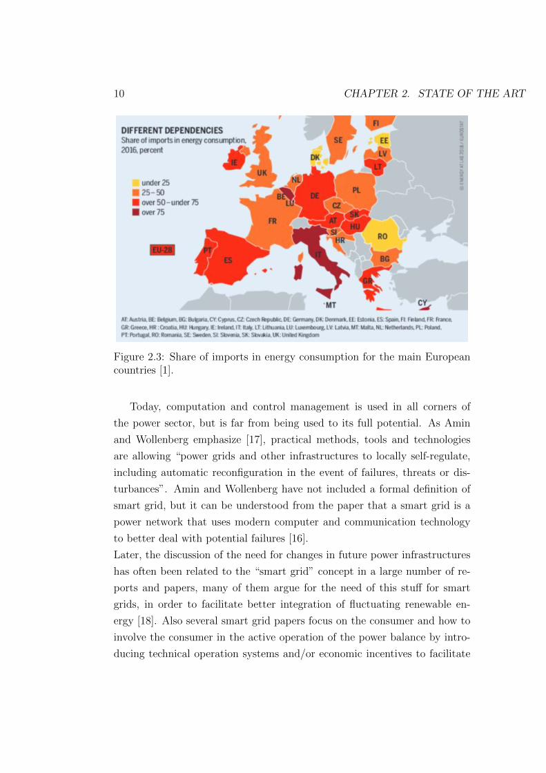
Despite progress with renewables, the European Union still imports 54 per-
cent of its energy needs, including 90 percent of its crude oil and 69 percent
of its natural gas. This import dependency comes at a high price: in 2013,
the EU spent 403 billion euros for fuel imports, falling to 261 billion euros
in 2015; this drop does not reflect lower demand but a fall in world market
prices-indicating the EU’s vulnerability to price volatility. In Fig. 2.3 we can
observe the share of imports in energy consumption for the main European
countries.
2.1.2 Smart energy systems and smart grids
In recent years, the terms “Smart Energy” and “Smart Energy Systems” have
been used to express an approach that reaches broader than the term “Smart
grid”. Where Smart Grids focus primarily on the electricity sector, Smart
Energy Systems take an integrated holistic focus on the inclusion of more
sectors (electricity, heating, cooling, industry, buildings and transportation)
and allow for the identification of more achievable and affordable solutions to
the transformation of renewable and sustainable energy. So smart grids may
require significant expansion of grid and storage infrastructures, while smart
energy systems can succeed within existing grid and storage infrastructures
[16].
10 CHAPTER 2. STATE OF THE ART
Figure 2.3: Share of imports in energy consumption for the main Europeancountries [1].
Today, computation and control management is used in all corners of
the power sector, but is far from being used to its full potential. As Amin
and Wollenberg emphasize [17], practical methods, tools and technologies
are allowing “power grids and other infrastructures to locally self-regulate,
including automatic reconfiguration in the event of failures, threats or dis-
turbances”. Amin and Wollenberg have not included a formal definition of
smart grid, but it can be understood from the paper that a smart grid is a
power network that uses modern computer and communication technology
to better deal with potential failures [16].
Later, the discussion of the need for changes in future power infrastructures
has often been related to the “smart grid” concept in a large number of re-
ports and papers, many of them argue for the need of this stuff for smart
grids, in order to facilitate better integration of fluctuating renewable en-
ergy [18]. Also several smart grid papers focus on the consumer and how to
involve the consumer in the active operation of the power balance by intro-
ducing technical operation systems and/or economic incentives to facilitate

2.1. BACKGROUND 11
flexible demands [16].
As showed in Fig. 2.4, the typical schema for defining a smart grid consists
Figure 2.4: Classical energy market compared to the one who use smart grids[1].
of a bi-directional power flow, i.e. the consumers also produce to the grid,
which differs from the traditional grid in which there is a clear separation
between producers on the one side and consumers on the other side resulting
in a uni-directional power flow. Consequently, concepts such as regulation
hierarchies, distributed generation (the challenge of integrating fluctuating
renewable energy sources into the electric power grid), vehicle to grid con-
cepts (charging systems capable of transferring energy not only from the

12 CHAPTER 2. STATE OF THE ART
source to the battery but also in the opposite direction, so that, if necessary,
the cars themselves can be transformed into reserves to draw on at particu-
larly critical moments to stabilize the network and avoid overloads) as well as
many micro-grids all become smart grids or part of the smart grid concepts
[1].
In 2013, [19] made a formal definition of a smart energy system con-
sisting of “new technologies and infrastructures which create new forms of
flexibility”. In simple terms, this means combining the electricity, thermal,
and transport sectors so that the flexibility across these different areas can
compensate for the lack of flexibility from renewable resources such as wind
and solar.
The smart energy system is built around three grid infrastructures:
• Smart Electricity Grids to connect flexible electricity demands such
as heat pumps and electric vehicles to the intermittent renewable re-
sources such as wind and solar power.
• Smart Thermal Grids (District Heating and Cooling) to connect the
electricity and heating sectors. This enables the utilisation of thermal
storage for creating additional flexibility and the recycling of heat losses
in the energy system.
• Smart Gas Grids to connect the electricity, heating, and transport
sectors. This enables the utilisation of gas storage for creating addi-
tional flexibility. If the gas is refined to a liquid fuel, then liquid fuel
storage can also be utilised.”
Based on these fundamental infrastructures, a smart energy system is defined
as follows: ”A Smart Energy System is defined as an approach in which smart
electricity, thermal and gas grids are combined with storage technologies and
coordinated to identify synergies between them in order to achieve an optimal
solution for each individual sector as well as for the overall energy system.”
Several synergies can be achieved by taking a coherent approach to the com-
plete smart energy system compared to looking at only one sector. This does
2.1. BACKGROUND 13
not only apply to finding the best solution for the total system, but also to
finding the best solutions for each individual sub-sector [16].
2.1.3 Microgrid
Following a decrease in the cost of batteries, the installation of residential,
stationary battery energy storages (BES) has increased, signifying their value
in reducing the electricity cost of the prosumers. BES can be combined with
residential PV to increase the self-supply level of end-users during the day
and can help small-scale RES owners increase their revenue by maximizing
self-consumption of PV generation [7].
The coupling of small-scale generation with residential BES could promote
the integration of microgrids (MG), i.e., clusters of local energy sources,
energy storages, and customers which are represented as a single control-
lable entity. The U.S. Department of Energy has defined the MG as [20]: ”a
group of interconnected loads and distributed energy resources within clearly
defined electrical boundaries that acts as a single controllable entity with re-
spect to the grid. A microgrid can connect and disconnect from the grid to
enable it to operate in both grid-connected or island mode.”
MGs can be employed at various locations including both rural and urban
areas. Off-grid solutions are usually ideal for remote rural areas. In cities, on
the other hand, grid-connected MGs can be formed by clusters of distributed
energy resources that are integrated in commercial or residential buildings [7].
2.1.3.1 Energy management
MGs are defined as clusters of distributed energy sources (generation, stor-
age, flexible loads, etc.) and energy consumers (non-flexible load): in grid-
connected mode, the difference between the MG generation and consumption
can be imported or exported to the main grid; while, in island mode, the MG
is completely autonomous meaning that energy is supplied exclusively from
the MG resources and any excess in generation must be stored or curtailed,
if self-consumption is not an option. In Fig. 2.5 we show a general micro-

14 CHAPTER 2. STATE OF THE ART
grid base structure with the DMS (Distribution Management System) of the
main grid that interact with the EMS (Energy Management System) of each
microgrid ( µ stands for one of the microgrids connected to the main grid).
Regardless of the mode of operation, a MG can be considered as a con-
Figure 2.5: Microgrid standard structure [2].
trollable entity, which is represented as a single entity to the distribution
grid. This can be achieved with the help of the MG controller, which is the
key component of the MG in control of the producing and consuming units
(distributed generation, flexible loads, storage) that are clustered together to
form the MG. The MG controller ensures that the operation of the MG is
both secure and reliable as well as efficient and economical.
The MG-EMS is employed by the MG controller and its main task is to
optimally balance load and supply both in the planning phase and in the
delivery phase (either by MG resources or through interconnections). The
use of the MG-EMS is essential in dispatching the MG resources in an in-
telligent, secure, and reliable manner and in achieving coordination both
among the MG components as well as with other grids. The objectives and
strategies that determine the decisions of MG-EMS are defined by the MG
operator. If the MG operator is different from the DSO and the MG operates

2.1. BACKGROUND 15
in grid-connected mode, then these objectives might not be co-aligned with
the operational objectives that optimize the operation of the main distribu-
tion network [7].
For example, if the objective for the DSO is to reduce the costs paid to
the TSO (thus minimising transmission costs), the whole grid operational ob-
jective for the DSO will be to make the microgrids as autonomous as possible
in such a way that they do not trade on the general distribution grid; for the
individual microgrids (MG operator) however the objective may be different,
e.g. in the case of profit maximisation the MG controller will inform the
MG-EMS to export as much energy as possible out of the microgrid, load-
ing the distribution grid and thus raising the transmission costs for the DSO.
The MG-EMS also determines the power exchange between the MG and
the main grid at the point of common coupling (PCC), which is the physical
interface of the MG with the distribution network. The operation between
multiple grid-connected MGs and the distribution network can be coordi-
nated by controlling the active (and/or reactive) power exchange at the
PCCs, but to achieve this level of coordination, a control and communi-
cation MG interface should be developed as an add-on DMS functionality to
integrate the MG energy scheduling with the network optimal power flow (a
functionality already available at the DMS) [7].
2.1.3.2 Optimal energy scheduling
The MG energy scheduling is the result of a decision-making process, where
the MGs and the DSO (or a MG aggregator) need to exchange information to
determine the interactions between the MGs and the main grid (e.g., power
exchange, energy prices). In this decision making process, there is often a
hierarchy with the DSO usually acting as the leader (upper level) and the
MG operators are the followers (lower level), then this problem can be for-
mulated as a bi-level optimization problem [7].
In most works presented in 2.1.3.1, the DSO is viewed as a supervisor and

16 CHAPTER 2. STATE OF THE ART
central coordinator for the energy exchange among all interconnected net-
work entities. Therefore, these studies usually assume that the DSO has full
knowledge of MG information, which extends beyond the PCC data such as
the MGs’ objectives, MG grid constraints as well as DER and customer data
in order to solve the bi-level optimization problem. Full knowledge helps
to simplify the bi-level optimization problem, as it can then be transformed
into an equivalent single-level mathematical problem with complementarity
constraints. Full MG information, however, comes into conflict with the
requirement of preserving the privacy of the MG data [7].
2.1.4 Internet of things
Internet of Things (IoT) refers to the networked interconnection of every-
day objects. It is described as a self-configuring wireless network of sensors
whose purpose would be to interconnect its nodes and deliver the informa-
tion to where it should be processed. Internet of Things has three important
characteristics:
1. Comprehensive sense, provided by the usage of sensors to collect infor-
mation of objects anytime, anywhere.
2. Reliable transmission, i.e. accurate real-time delivering information of
objects through meshing a variety of telecommunications networks and
Internet.
3. Intelligent processing, i.e. using intelligent computing such as cloud
computing to analyze and process vast amounts of data and informa-
tion, for the purpose of implementation of intelligent control to objects.
IoT has some use cases in intelligent environmental protection (an im-
portant long-term strategy of national development), as the massive envi-
ronmental data including water data, air data, regional environment data,
nature protection data and other data, should be collected accurately by
sensors and transmitted to servers to be treated and analyzed by software.
The intelligent environmental protection includes intelligent environmental

2.1. BACKGROUND 17
monitoring, intelligent public facilities monitoring, intelligent city pipeline
monitoring, intelligent sewage treatment monitoring, intelligent parks con-
trol and so on [21].
2.1.4.1 IoT role in smart grid technology
Smart Grid is a new kind of intelligent power system realized with infor-
mation, communication, the computer control technology and the existing
transmission/distribution power infrastructure. The applications of IoT in
the Smart Grid are divided into smart power generation, intelligent trans-
mission and substation and intelligent power use, data collection is the key
to smart power grid. Sensor technology in IoT forms interactive real-time
network connection between the users, corporation and power equipment to
make data reading real-time, high-speed and two-way, which improve the
overall efficiency of the integrated power grid [22]. Smart Grid may use
more devices, including a variety of intelligent sensors, control components
and electrical equipment, which require higher digitization degree of power
grid and better data collection, transmission, storage and utilization in the
process of power generation, transmission, substation and distribution [21].
2.1.4.2 IoT edge cloud architecture
An IoT edge cloud architecture (see Fig. 2.6) is a distributed system, typ-
ically consisting of an outer rim of IoT, sensor devices and networks, an
intermediate layer of local processing capabilities and more centralised cloud
systems for data processing and storage. Fog and edge architectures provide
a link between centralised clouds and the world of IoT and sensors. The
architectures consist of devices of different sizes that coordinate the commu-
nication with sensors and cloud services, and that process data from or for
the sensors and the cloud locally [23].
The next generation of factories will be digital, it will mostly work au-
tonomously and will adapt its production processes dynamically in order to
improve the product quality, detect machine failures, etc. This is fueled by
the integration in real time of big data, edge and cloud computing, analytics,

18 CHAPTER 2. STATE OF THE ART
Figure 2.6: The edge computing infrastructure.
machine learning and networks. For this purpose, the machines will have
numerous sensors and actuators, which detect, perceive and they act in real
time with a significant level of autonomy and adaptation. For this, artificial
intelligence and machine learning methods are very important. To adapt
quickly, intelligence must be close to machines, spreading analytical intelli-
gence on ”network-edges”, to run AI algorithms inside the factory both on
small integrated boards near the machines and on larger computing nodes
within the factory’s IT services. This edge/cloud-based architecture requires
reliable and real-time communication and custom hardware/software in local
controllers to support large-scale AI-based applications that can work with
temporal constraints [24].

2.1. BACKGROUND 19
Smart grids employ smart meters which are responsible for two-way flows
of electricity information to monitor and manage the electricity consumption.
In a large smart grid, smart meters produce tremendous amount of data that
is hard to process, analyze and store. The regular monitoring is expected to
be performed with all kinds of IoT devices and processing servers instead
of manpower, where IoT devices such as sensors and cameras will collect
and upload the real-time videos and other information about the power line
to the processing servers. Such information will then be automatically pro-
cessed by the servers running ML algorithms to detect potential threats and,
if necessary, trigger appropriate actuations to achieve timely and intelligent
monitoring with automatic threat identification.
Since deep learning algorithms are extremely data intensive, computation
intensive and hardware-dependent, the processing servers of smart grid are
expected to be equipped with abundant computation resources. This makes
cloud computing be widely proposed as a natural choice to host such servers.
However, transferring large volume of data into the cloud will push significant
pressure to the network and generate huge communication costs. In addition,
from power providers perspective, moving data to the remote cloud may also
incur privacy concerns. Moreover, the latency in the network can become
a severe performance bottleneck due to the latency sensitivity of real-time
monitoring.
Recently, the concept of edge computing has been proposed as a comple-
ment of cloud computing, attracting great interests from both academia and
industry. In contrast to cloud, edge usually refers to a geographical concept
which is in close proximity to the end devices in the network [25]. By pushing
applications, data and services away from centralized cloud to edge servers,
the computing paradigm will be extended to an edge-cloud collaborative com-
puting, which has shown outstanding performance on communication latency
and traffic reduction, and ease the privacy concerns of users as well [26].
In conclusion, edge computing is an environment that offers a place for col-
lecting, computing and storing smart meter data before transmitting them to

20 CHAPTER 2. STATE OF THE ART
the cloud. This environment acts as a bridge in the middle of the smart grid
and the cloud. It is geographically distributed and overhauls cloud comput-
ing via additional capabilities including reduced latency, increased privacy
and locality for smart grids [27].
2.2 Related Works
2.2.1 Existing Microgrid-based Energy Management
Systems models
Traditionally, energy consumers pay non-commodity charges (e.g. transmis-
sion, environmental and network costs) as a major component of their energy
bills. With the distributed energy generation, enabling energy consumption
close to producers can minimize such costs. The physically constrained en-
ergy prosumers in power networks can be logically grouped into virtual mi-
crogrids (VMGs) using communication systems.
There are centralized and distributed optimization approaches: distributed
approaches are, for example, based on game theory as no global information
is available and each agent makes its own decisions. Peer-to-peer (P2P) en-
ergy trading offers an approach to produce and sell energy at the edge of the
network and can help in reducing charges. Since there are multiple producers
and consumers involved, attaining optimal pricing as well as utility for the
consumers and producers respectively, can be complicated.
[28] introduces a game theory-based approach to optimize energy trading
costs in a single VMG. In this work prosumers can act as consumers when
they need to buy energy. In the model, A (a producer) sets up its own
energy price and the consumer has the liberty to choose who to purchase
energy from. Typically, the energy price defined by A is cheaper than the
grid-price at the prevailing transaction interval. Thus, the price set by A
depends on the prices set by other A’s and the grid. This type of coupling
between prosumers’ trading strategies necessitates the use of game theory to
model the interaction between the producers and consumers. Specifically, is
adopted a multi-leader multi-follower Stackelberg game.
2.2. RELATED WORKS 21
For [3] there are some reasons game theory is applied to model the energy
management of future distribution networks with the presence of multiple
microgrids, the main reasons for authors to use game theory in this problem
have been listed as follow:
• The strategic game is used to model selfish behaviors of other agents.
• Networked optimization usually consists of multiple agents who can
observe and react to their environment. Game theory offers a powerful
tool set to analyze interactions between such intelligent entities.
• Although network components or agents would like to cooperate, it
might be impractical or impossible to exchange the information re-
quired to implement presented method. It might then be better for
agents to optimize their local or private objective and react to limited
network information.
• Game theory provides a way to predict, analyze or even to improve the
outcome of a non-cooperative interaction, e.g. the notation of equilib-
rium.
[3] present optimal scheduling of resources from the DNO’s point of view con-
sidering reaction of multiple autonomous microgrid; since multiple microgrid
are considered multi follower bi-level programming has been implemented.
In general, MFBP is a bi-level decision-making problem which has three sig-
nificant characteristics:
• There exists two decision levels within a principally ordered structure.
• The decision level at the lower order executes its policies in consequence
of decision making at the upper level.
• Each level autonomously optimizes its objective but it is affected by
the reactions of other level.

22 CHAPTER 2. STATE OF THE ART
The decision maker at the upper level is denominated as the leader, and at
the lower level, is named as the followers. The leader cannot adequately
control the decision making process of the followers, however, it is affected
by the reaction of the followers. The optimal solution of the followers allow
the leader to execute his/her objective functions value. Since, this type of
decision making process has been appeared in many decentralized organiza-
tions, and been mainly handled by bi-level programming technique.
As shown in the Fig. 2.7 the problem has been formulated in two level witch
DNO as upper level determines its decision making considering reaction of
MGs.
Figure 2.7: Problem statement as a bi-level programming [3].
For [29], a critical point for the distributed management can be that each
microgrid control centre is not informed of generated and consumed powers
of other rivals, consequently, the microgrids may face the problem of common
line congestion.
Assuming a line limitation in PCC and some microgrids are connected to
the grid through this point. When grid electricity price is cheap/expensive,
each microgrid starts to buy/sell from/to grid without knowing about neigh-
bouring microgrids. For this purpose, in this work, a new unit to manage
congestion called MGA is proposed. This unit is responsible for line utilisa-
2.2. RELATED WORKS 23
tion, and allocating fair capacity among various microgrids.
The proposed mathematical framework for solving the problem is based on a
bi-level model: in the first level, microgrids implement day-ahead scheduling
independently and provide the aggregator with the results; In the second
level, a novel energy management mechanism is carried out by the aggrega-
tor, taking PCC constraints into consideration.
[30] and [31] formulate the problem as a stochastic bi-level problem with
the DNO in the upper level and MGs in the lower level and also for [32]
the MMG system is a hierarchical decentralized SoS. Individual MGs are in-
dependently managed and operated, and they can choose to join the MMG
system, but a controller for the MMG system, the DMS, is present to coordi-
nate the power exchange among the participating MGs and the trading with
the DN. Energy management at the level of MMG system interacts with the
DN and coordinates participating MGs in the system. In other words, the
MGCC of each participating MG derives an optimal solution of energy man-
agement for the MG with consideration of the request for power exchanges
and trading from the DMS. Meanwhile, the DMS assesses the optimality of
energy management solutions for the MMG system based on the optimal
solutions provided by the MGCCs.
The development of a cluster-based (similar to microgrid) energy manage-
ment scheme with a mathematical model for residential consumers of a smart
grid community is proposed by [33] to reduce energy use and monetary cost.
Solar and wind generators, an energy storage system and a typical energy
consumption profile for residential consumers are also considered. Further-
more, the home appliances considering peak-load, mid-peak, and off-peak
loads and real-time electricity prices scenarios are modeled.
However, we highlight that most models take into account a ”simplified”
microgrid structure (see Fig. 2.8) only with ”produce” and ”consume” agent-
types, in which the prosumer entity (an agent that both ”produce” and
”consume”) is not present.
The energy scheduling problem illustrated in the work [7] takes into con-

24 CHAPTER 2. STATE OF THE ART
Figure 2.8: Standard MG system communication infrastructure, linking themicrogrid central controller (MGCC) and the local controllers (LCs) [4].
sideration the prosumer entity and, respect to all the others works that
mostly focus on the dynamic prices based on supply/demand, this estab-
lish fixed prices (considered in the decision making process) and the main
issue is the energy exchange between the microgrid agents. For this reason
this was chosen as the starting point for the optimization component in this
work.
2.2.2 Microgrid Energy Management optimization prob-
lem
The energy management in microgrids is typically formulated as an offline op-
timization problem for day-ahead scheduling, most of the offline approaches
assume perfect forecasting of the renewables, the demands, and the mar-
ket, which is difficult to achieve in practice. Existing online algorithms,
on the other hand, oversimplify the microgrid model by only considering
the aggregate supply-demand balance while omitting the underlying power
distribution network and the associated power flow and system operational
constraints. Consequently, such approaches may result in control decisions
that violate the real-world constraints [4].

2.2. RELATED WORKS 25
2.2.3 Real-world Deployments of Microgrid Energy Man-
agement Systems
MG-EMSs are already offered by several manufacturers including Siemens,
Hitachi, and General Electric among others. Some of these platforms provide
also integration with the supervisory control and data acquisition (SCADA)
system of the utility through standard industrial protocols. Thus, the tech-
nology for both MG deployment and DSO integration is available. The adop-
tion of MGs could benefit both end-users, which could reduce their energy
cost, and the operation of the distribution system, which can exploit the
energy flexibility offered by MGs [7].
2.2.3.1 Siemens
Microgrid Control Microgrid Control from Siemens provides reliable con-
trol and monitor a microgrid, ensuring an independent power supply and bal-
ancing out grid fluctuations as well as fluctuations in energy consumption,
the Fig. 2.9 illustrates the components over which control is exercised [5]. It
offers the following functionalities:
• Blackout detection, black start, and automatic grid modes;
• Automatic start of backup generators;
• Optimization of operating points;
• Reserve monitoring;
• Peak shaving;
• State-of-charge management.
Spectrum Power™ Microgrid Management System The Siemens Spec-
trum Power™ MGMS is an advanced control and optimization software – used
to maximize the value of onsite generation and energy storage in coordina-
tion with local utility rates, it can be used as a support tool for the more

26 CHAPTER 2. STATE OF THE ART
Figure 2.9: Microgrid Control, by Siemens [5].
general Microgrid Controller. Spectrum Power™ has the ability to forecast
site electrical and thermal loads – and while taking into account the cur-
rent electric and fuel/gas utility tariffs, will execute a comprehensive plant
operation routine in order to find the economic optimal unit schedules for
the next 24 hours or 7 days. These schedules are then dispatched in real
time, turning units on and off, and sending the economic optimal operating
set points and charge/discharge rates. This results in significantly decreased
operating expenses from electricity and fuel/gas purchases.
The overall function of MGMS (as showed in Fig. 2.10) is the optimal coor-
dination of dispatchable generation (gas, diesel generators, etc.), renewable
generation (PV, wind, etc.), energy storage (batteries), and load (via Build-
ing Management System or remotely-operated switches) [6].
2.2.3.2 Hitachi e-mesh Energy Management System
Hitachi ABB Power Grids’ e-mesh™ EMS is specially designed to manage
distributed energy and renewable resources, conventional power generation
sources, and controllable loads like electric vehicle chargers. e-mesh EMS is
a flexible and highly scalable application that allows for easy expansion as

2.2. RELATED WORKS 27
Figure 2.10: MGMS Operational Flow, by Siemens [6].
the number of energy resources and the size of the operation grow [34].
The application comes with four key features:
• EMS Optimize: improves energy production whilst reducing costs and
emissions. With the optimisation module the assets’ management is
based on each unit’s constraints and costs. Flexible and scalable models
are implemented to rapidly expand from few to several units.
• Simulate & Plan: helps in making cost-effective decisions.
• Analyze: enhances transparency whilst providing energy insights.
• Integrate: enables connectivity options for integration with SCADA
(”Supervisory Control And Data Acquisition”) systems, third-party
systems such as forecast providers and trade platforms can also be easily
integrated with the application, allowing meaningful data exchange.
2.2.4 Identified research gaps
At present there are many practical and theoretical solutions that adopt
the technique of optimisation in distributed systems using e.g. game theory
which do not assume global knowledge, while there are missing centralised

28 CHAPTER 2. STATE OF THE ART
solutions that can calculate good solutions fast.
In addition, we would like to avoid using off-the-shelf products, this to
ensure maximum low coupling between the various components from the very
beginning of the project, in such a way that you can test the performance and
add, modify or remove components when necessary (for research purposes of
new solutions, testing for machine learning models, etc.).
As [7] has observed, studies on coordinated operation of the MGs and
the DSO have exclusively focused on defining the amount of energy trade
between the DSO and the MGs often without considering the underlying
constraints of the distribution network operation.
For efficient BES dispatch and accurate evaluation of the BES utilization, it
is important to consider both real-life performance and usage constraints of
the BES for each prosumer.

Chapter 3
Design
This chapter first presents the general structure of the existing context in
which we operate. It then illustrates the software architecture designed to
manage and process the data, irrespective of the technologies used. This
is followed by a presentation of the data sources used for the simulations,
the machine learning model used to derive the energy production data, the
theoretical structure of the energy scheduling problem and, finally, the per-
formance metrics chosen for the subsequent evaluation phase.
3.1 Energy network structure
The Fig. 3.1 shows the basic general structure of the smart grid on which
the project will be developed.
Each microgrid contains a cluster of prosumers, each with an associated
control board (edge unit) that is responsible for collecting data from the
various sensors (battery state of energy, energy consumption and energy pro-
duction from the photovoltaic panels) and for receiving any instruction for
the battery scheduling from the controllers. In the cloud we find the micro-
grid controllers, which are responsible for collecting all local information and
making optimal decisions at a global level (such as how much energy each
prosumer has to draw/feed from/into its battery); the main grid provides
other information such as energy buying and selling prices etc. and a circuit
29

30 CHAPTER 3. DESIGN
Figure 3.1: Network structure with microgrids. In the microgrid (i) in thescheme there are j prosumers.

3.2. GENERAL SYSTEM ARCHITECTURE 31
breaker acts as an automatically operated electrical switch.
As illustrated in the legend, there are two ”parallel” flows:
• the energy flow that, starting from the main grid, branches out on
the electricity grid and arrives at each prosumer (this configuration is
independent of the microgrid as the latter is intended to represent an
abstract level cluster only);
• the flow of information (depending on the configuration of the prosumer
cluster in the microgrid) which can be divided into two phases: sending
data to the server and receiving results/decisions.
3.2 General system architecture
Based on the structure illustrated in the previous section, the hardware/-
software system in Fig. 3.2 has been designed to achieve the objective of
this project: each prosumer predicts its energy supply and demand locally
using edge computing and pushes this information to the cloud that, in a
marketplace, optimize energy exchanges between prosumers.
Each edge unit receives the data from the sensors and, together with those
values, it sends to the server (as telemetries) also the data predicted by the
machine learning model for the next time interval. In the cloud server, the
data is received by a device manager that passes it to an aggregator that
groups together all the time series data-points received in a certain time in-
terval for each microgrid; the aggregated real-time data are sent to a tool
for graphical representation (consumption and production), while the aggre-
gated data becomes the input for the energy scheduling optimizer. The result
of the optimisation (which devices should charge or discharge their battery
in the next time interval) is finally communicated to the respective boards.
3.2.1 Data structure in the flow
The table 3.1 shows the structure of the data collected and sent (in out
use case, sent every 30 seconds) from the board (edge unit) to the server.

32 CHAPTER 3. DESIGN
Figure 3.2: General system architecture. In this schema is represented, asan example, only one edge unit (i).
Depending on the strategy used (local or global, see section 3.5 for a detailed
explanation) some of these fields may be empty or not.
This data structure is similar even after aggregation for each device and
then for each microgrid; indeed, the output of the aggregator contains the
attributes concerning the individual prosumer together with the ones of the
microgrid. As showed in table 3.2, the data that regard a property of the
single device are the ones with index: 1, 2, 7, 9, 10; while the ones which are
an aggregation of the values produced by the board in a 5-minute interval
have index: 3, 4, 5, 6, 8, 11, 12. Data such as consumption and production are
aggregated by summing all the data-points while the battery state of charge
is averaged over the 5-minutes interval. The attribute microgridAggregator
(index 13) has the structure represented in table 3.3 and contains the sum (for
that precise time interval) of consumption, production, import and export
for the microgrid stated in microgridID (index 1) and is replicated in every
device belonging to that microgrid.

3.2. GENERAL SYSTEM ARCHITECTURE 33
Index Data Source Strategiesthat usethe data
1 microgridID board local,global
2 deviceID board local,global
3 consumption (kW): energyconsumption of the buildingin the previous time step
sensor local,global
4 production (kW): energyproduction of the PVs in theprevious time step
sensor local,global
5 predictedConsumption(kW): predicted energyconsumption of the build-ing for the next timestep
ML inference global
6 predictedProduction (kW):predicted energy produc-tion of the PVs for the nexttime step
ML inference global
7 batteryCapacity (Ah) battery at-tributes
global
8 batteryStateOfCharge (Ah) sensor global9 chargingLimit (percentage):
maximum amount of bat-tery charge for a time step
battery at-tributes
global
10 dischargingLimit (percent-age): maximum amount ofbattery discharge for a timestep
battery at-tributes
global
11 energyImport (kW) local computa-tion
local
12 energyExport (kW) local computa-tion
local
Table 3.1: Data structure from the board.

34 CHAPTER 3. DESIGN
Index Data Strategies thatuse the field
1 microgridID local, global2 deviceID local, global3 sumConsumption (kW) local, global4 sumProduction (kW) local, global5 sumPredictedConsumption (kW) global6 sumPredictedProduction (kW) global7 batteryCapacity (Ah) global8 averageBatteryStateOfCharge (Ah) global9 chargingLimit (percentage over the battery
capacity)global
10 dischargingLimit (percentage over the bat-tery capacity)
global
11 sumEnergyImport (kW) local12 sumEnergyExport (kW) local13 microgridAggregator local
Table 3.2: Data structure of the output of the aggregator (for each device).
Index Data
1 microgridID3 sumConsumption (kW)4 sumProduction (kW)5 sumEnergyImport (kW)6 sumEnergyExport (kW)
Table 3.3: Data structure of the attribute microgridAggregator.
3.3 Input data preparation
For this project it has been decided to simulate consumption and production
data, in order to create prosumers with different profiles (e.g. residential
or commercial), otherwise connecting real sensors to the board would have
simulated at most one single prosumer at a time.
A number of datasets containing numbers on energy consumption and pro-
duction over the course of a day have been then used to simulate real data.
3.3. INPUT DATA PREPARATION 35
3.3.1 Datasets
3.3.1.1 Production
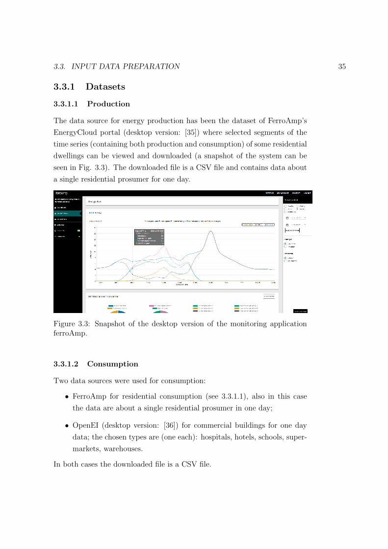
The data source for energy production has been the dataset of FerroAmp’s
EnergyCloud portal (desktop version: [35]) where selected segments of the
time series (containing both production and consumption) of some residential
dwellings can be viewed and downloaded (a snapshot of the system can be
seen in Fig. 3.3). The downloaded file is a CSV file and contains data about
a single residential prosumer for one day.
Figure 3.3: Snapshot of the desktop version of the monitoring applicationferroAmp.
3.3.1.2 Consumption
Two data sources were used for consumption:
• FerroAmp for residential consumption (see 3.3.1.1), also in this case
the data are about a single residential prosumer in one day;
• OpenEI (desktop version: [36]) for commercial buildings for one day
data; the chosen types are (one each): hospitals, hotels, schools, super-
markets, warehouses.
In both cases the downloaded file is a CSV file.

36 CHAPTER 3. DESIGN
3.3.2 Pattern extraction
For both consumption and production it has been decided to find the daily
pattern. For each time series of data (residential production/consumption
and commercial) hourly mean and standard deviation have been calculated
over a single prosumer, starting from a data granularity of 1 minute.
Arithmetic mean and standard deviation have been computed as well:
x =1
N
N∑i=1
xi (3.1)
s =
√√√√ 1
N − 1
N∑i=1
(xi − x)2 (3.2)
because, when looking at various graphs and/or time series representing pro-
duction and/or consumption values, it was noted that the values follow a
normal distribution (see figures 3.4 and 3.5).
Having these two values for each hour, the simulator generate a significant
value (a normally distributed random number) for any time of day and at
any granularity (depending on the frequency chosen for sending telemetry
from the board to the server) proportioning the values to the granularity of
the original dataset.
3.4 ML model for production inference
In our case, a 4-layer bidirecional LSTM model (from[38]) has been used to
infer the energy production of the photovoltaic panels.
In comparison to normal MLP (Multilayer Perceptron), which consists of
many layers with neurons in it and the input data is propagated through the
network itself, the LSTM (Long Short-Term Memory Network) has recurrent
connections. This means, that the state of the previous activations is also
used as a context for the output. Long short-term memory (LSTM) is, in
fact, an artificial recurrent neural network (RNN) architecture mostly used in
the field of deep learning and, unlike standard feedforward neural networks,

3.4. ML MODEL FOR PRODUCTION INFERENCE 37
(a) Average daily energy consumption during the weekdays and the variationthroughout the different months [37].
(b) Average daily energy consumption during the weekdays and the variationthroughout the different months [37].
Figure 3.4: Average daily energy consumption and the variation throughoutthe different months.

38 CHAPTER 3. DESIGN
(a) Average monthly load profiles of the block of flats from January to June [37].
(b) Average monthly load profile of the block of flats from July to December [37].
Figure 3.5: Average monthly load profiles of the block of flats.

3.5. STRUCTUREOF THE ENERGY SCHEDULING PROBLEMAND SOLUTION APPROACHES39
LSTM has feedback connections, this means that it can not only process
single data points (such as images), but also entire sequences of data (such
as speech or video). In addition, in comparison to normal RNN the design
of the LSTM Network allows to overcome the problem of the vanishing or
exploding gradients ( the weight update procedure changes the weights so fast
in one direction or the other, that it is graduate to zero or infinity) as those
phenomena make the neural network useless. Moreover, in general RNNs are
good for the processing of sequential data and for the prediction of those, but
those networks suffer from short-term memory. LSTM networks overcome
this obstacle processing a time series one step at a time and maintaining an
internal state that summarises the information acquired up to that moment
[38].
A Bidirectional LSTM, or biLSTM, is a sequence processing model that
consists of two LSTMs: one taking the input in a forward direction, and the
other in a backwards direction. BiLSTMs effectively increase the amount of
information available to the network, improving the context available to the
algorithm (e.g. knowing what words immediately follow and precede a word
in a sentence) [39]. In Sec. 4.6 the technical details of the model for inference
will be explained.
3.5 Structure of the energy scheduling prob-
lem and solution approaches
The solution of the MG energy scheduling problem depends on the opera-
tional objectives of the MG operator. It is assumed that the MG operator
has full access to the installed DERs in the MG and is responsible for deliv-
ering power to the MG customers; the MG operator is a different entity from
the DSO.
The architecture proposed by [7] for the integration of the MG to the distri-
bution system can be seen in Fig. 3.6, which is a schematic representation of
the interface between the MG-EMS and the DMS. Two-ways communication
is always assumed between the MG-EMS and the DMS. No communication or

40 CHAPTER 3. DESIGN
interaction is considered between different MG-EMSs, i.e., the MG-EMSs can
only interact with the DMS. Three different schemes of coordination between
the MG-EMS and the DMS are depicted, these coordination schemes, which
affect the approach followed for the solution of the MG energy scheduling
problem, can be described as follows:
• No coordination: the MG-EMS solves the energy scheduling problem
and dispatches the MG resources according to this solution.
• Centralized coordination: it is assumed that the DMS is empowered
to dispatch the MG resources, the MG-EMS receives the reference set-
points from the DMS and then transmits them to the MG resources.
• Decentralized coordination: the DMS can only transmit the desired
reference values for the PCC and is in no other way involved in the
MG energy scheduling.
In our use case we have decided to use ”No coordination” for the two global
strategies (see Sec. 3.5.3).
3.5.1 Rolling horizon
An energy management scheme can have a scheduling horizon that depends
on the accuracy of the forecasted values of load, non-dispatchable generation
and electricity price. It can be applied hour-ahead, day-ahead, week-ahead
or even month-ahead. The scheduling horizon is divided in time steps (time
discretization steps), which usually (although not necessarily) correspond to
the frequency update of the dispatched set-points and the resolution of the
input data (resolution of forecast).
Typically, hourly or 15-minutes time intervals are used in energy manage-
ment. Energy management schemes with time intervals which are shorter
than 5 minutes can be classified as real-time energy management schemes.
For implementation of real-time or close to real-time energy management,
the rolling horizon (RH) approach must be adopted. When the MG energy
scheduling follows a RH approach, the energy scheduling problem is solved

3.5. STRUCTUREOF THE ENERGY SCHEDULING PROBLEMAND SOLUTION APPROACHES41
Figure 3.6: The integration of the MG-EMS to the DMS [7].
before each time step [7]. In our case, as we have a 5 minutes time step
(to determine the transactions between the components of the microgrid) we
have decided to use the rolling horizon approach in our scheduling problem.
As showed in Fig. 3.7, during the time step 1 (between t and t+1, where +1
means 5 minutes) together with the real time data, the board also sends the
predicted data (production and consumption) for time step 3 (between t+2
and t+3), because we take into account time step 2 as the time-frame for
the computation of the optimised energy scheduling; therefore the decisions
for time step 3 will be made based on data received in time step 1. This
procedure is performed at each time step, shifting 2 units for the results.
3.5.2 Business As Usual (local) strategy
In this scenario, the dispatch of the BES follows a rule-based algorithm local
to the edge unit; each prosumer then acts independently of the others and
charges/discharges its battery and buys/sells energy only according to its
needs. The procedure showed in the Algorithm 1 is actuated in each board,

42 CHAPTER 3. DESIGN
Figure 3.7: The rolling horizon approach.
in case the chosen strategy is the BAU (Business As Usual, normal execution
of operations will be followed) this will also be the final local configuration
of the edge-unit. The first step is to check whether the prosumer has an
energy deficit or surplus, after this the energy balance of the single prosumer
is levelled with two possible alternatives:
• charging (in case of surplus) or discharging (in case of deficit) the bat-
tery: in this case it is checked that this meets the conditions indicated
in the Equations 3.4, 3.5, 3.6, 3.7, 3.8;
• importing/buying (in case of surplus) or exporting/selling (in case of
deficit) energy: this solution is adopted if and only if the energy balance
has not been completely levelled out by using the battery.
More in detail, the Algorithm 1 adopts the following procedure to check that
the scheduling meets the conditions indicated in the Equations 3.4, 3.5, 3.6,
3.7, 3.8:
• At line 1 it calculates the difference between production and consump-
tion, if this value is positive the prosumer has a surplus of energy,
otherwise there is a deficit.
• In case of surplus (from line 6 to 20) it is checked if it is possible to
recharge the battery of that particular building for the entire amount
of the extra energy (line 7) based on the maximum charging level for a
time-step.

3.5. STRUCTUREOF THE ENERGY SCHEDULING PROBLEMAND SOLUTION APPROACHES43
– If the quantity does not exceed the maximum charging level (lines
8-13), it is checked that the maximum SoE for that prosumer
(corresponding to 80% of the battery capacity) is not exceeded
(line 8); if this value is surpassed, the feasible amount is stored in
the battery and the remaining amount is exported (lines 12-13).
– If the quantity exceeds the maximum charging level (lines 15-20),
it is checked that the maximum SoE for that prosumer is not
exceeded by just adding the maximum charge quantity (line 15);
if the maximum SoE is surpassed, the feasible amount is stored in
the battery and the remaining amount is exported (lines 19-20).
• In case of deficit (from line 22 to 36) it is checked if it is possible to
balance the entire amount of the deficit of energy by discharging the
battery of that particular building for of the based on the maximum
discharging level for a time-step (line 23).
– If the quantity does not exceed the maximum discharging level
(lines 24-29), it is checked that the minimum SoE for that pro-
sumer (corresponding to 20% of the battery capacity) is not ex-
ceeded (line 24); if this value is surpassed, the feasible amount is
drawn from the battery to be used and the remaining amount is
imported (lines 25-26).
– If the quantity exceeds the maximum discharging level (lines 31-
36), it is checked that the minimum SoE for that prosumer is not
exceeded by withdrawing the maximum discharge quantity (line
31); if the minimum SoE is surpassed, the feasible amount is with-
drawn from the battery and the remaining amount is imported
(lines 19-20).
3.5.3 Optimized (global) strategies
The MGs can have different objectives (minimize the exchange with the
main grid or minimize the total cost) and centrally (respect to the MG)
coordinated energy scheduling (microgrid global optimization) is considered

44 CHAPTER 3. DESIGN
in this case. Depending on the strategy (operational objectives), a different
energy scheduling problem is formulated and solved.
The optimisation strategies are addressed to the single microgrid, foreseeing
energy exchanges only between prosumers within the same microgrid and not
between those belonging to different microgrids; outside the cluster there are
exchanges only with the DSO and the microgrids do not cooperate with
each other. We are not looking at individual prosumer exchanges within a
microgrid and we assume that they all cooperate because, otherwise, there
should be a rationale about what should be doe with surplus of money of the
microgrid, how should that be distributed to individual prosumers and which
prosumers are willing to exchange energy with others. This problem is solved
by the MG-EMS of each individual MG. However, the solution can also be
affected (or even directly dispatched) by the DMS of the DSO depending on
the level of interaction between the MGs and the DSO (in our case the only
interaction consist in communicating the energy prices).
3.5.3.1 General constraints
MG energy balance In 3.3, C is the set/cluster of prosumers in that
microgrid, pim and pex are its import and export. For each prosumer j,
bch, bdis respectively refer to the charging/discharging of his battery, pPV is
his photovoltaic energy production and pC is his energy consumption. This
constraint is necessary to ensure that the energy balance in the individual
microgrid is maintained.∑j∈C
(pPVj,t − pCj,t − bchj,t + bdisj,t ) + pim − pex = 0 (3.3)
BES scheduling The BES model that has been most frequently used in
the latest literature on BES scheduling (for [7]) assumes that the SoE of the
BES at each time step is linearly dependent on the cumulative BES through-
put of the previous time steps. This model is described by the following
equations:
soej,t = soej,t−1 + bchj,t−1 − bdisj,t−1,∀j ∈ C (3.4)

3.5. STRUCTUREOF THE ENERGY SCHEDULING PROBLEMAND SOLUTION APPROACHES45
SoEminj < soej,t < SoEmax
j ,∀j ∈ C (3.5)
0 ≤ bchj ≤ kchj , ∀j ∈ C (3.6)
0 ≤ bdisj ≤ kdisj ,∀j ∈ C (3.7)
bchj,t ∗ bdisj,t = 0,∀j ∈ C (3.8)
In the above formulation, C is the set/cluster of prosumers in that microgrid,
kch, kdis denotes the maximum charging/discharging power according to the
specifications of the battery manufacturer. Moreover, bch, bdis respectively
refer to the charging/discharging of the battery, SoE is the state-of-energy,
which must lie between the lower and upper limit (SoEmin and SoEmax, re-
spectively). It is also noticeable that the battery of a prosumer can only
be charged or discharged in a time step, is impossible having both values
different than 0.
3.5.3.2 Objective functions
Minimum exchange strategy In this case the objective function is the
energy exchange minimization and is related to the desired level of interaction
between the single microgrid and the main grid (as the microgrids do not
cooperate with each other).
min(pim + pex) (3.9)
46 CHAPTER 3. DESIGN
In 3.9, p is the power imported im and exported ex in that microgrid that
wants to minimize its energy exchange. These two variables are the result-
ing value for the entire microgrid after the energy deficits and surpluses of
the prosumers within it have been aligned and possibly compensated for by
charging and/or discharging the batteries.
Minimum cost strategy In this case the objective function is cost min-
imization for the single microgrid, which can alternatively be formulated as
profit maximization, and is related to economic operation targets.
min(pim ∗ P SLOT im − pex ∗ P SLOT ex
) (3.10)
In 3.10, p is the power imported im and exported ex in that microgrid that
wants to minimize its cost/maximize its profit and PSLOT is the price, given
by the main grid for import im and export ex. Also in this case pim and
pex are the resulting value for the entire microgrid after the energy deficits
and surpluses of the prosumers within it have been aligned and possibly
compensated for by charging and/or discharging the batteries, with the goal
of minimizing the cost.
3.6 Evaluation metrics
In order to evaluate the project, we consider in different scenarios the differ-
ences between the global optimisation strategies and the local BAU strategy.
For example, in the case of minimizing cost / maximizing profit, the cost
incurred by the microgrid in case of adoption of the global strategy will be
compared with the cost sustained in case of BAU. Different configurations
for the algorithms and their impact on the final performance (e.g. solving
times) will also be compared.

3.6. EVALUATION METRICS 47
Algorithm 1: BAU local algorithm
Data: prevBatterySoe, batteryCapacity,maxCharging,maxDischarging, production, consumptionResult: export, import, newBatterySoe
1 diff ← production− consumption;2 import← 0 ;3 export← 0 ;4 newBatterySoe← 0;5 if diff > 0 then6 charging ← diff ;7 if charging < maxCharging ∗ batteryCapacity then8 if (prevBatterySoe+ charging) < 0.8∗ batteryCapacity then9 newBatterySoe← prevBatterySoe+ charging;
10 export← 0;
11 else12 newBatterySoe← 0.8 ∗ batteryCapacity;13 export← charging− (newBatterySoe−prevBatterySoe);14 else15 if (prevBatterySoe+ (maxCharging ∗ batteryCapacity)) <
0.8 ∗ batteryCapacity then16 newBatterySoe←
prevBatterySoe+ (maxCharging ∗ batteryCapacity);17 export← charging − (maxCharging ∗ batteryCapacity);
18 else19 newBatterySoe← 0.8 ∗ batteryCapacity;20 export← charging− (newBatterySoe−prevBatterySoe);
21 else

48 CHAPTER 3. DESIGN
(21)
(22) discharging ← −1 ∗ diff ;(23) if discharging < maxDischarging ∗ batteryCapacity then(24) if (prevBatterySoe− discharging) < 0.2 ∗ batteryCapacity
then(25) newBatterySoe← 0.2 ∗ batteryCapacity;(26) import←
discharging − (prevBatterySoe− newBatterySoe);(27) else(28) newBatterySoe← prevBatterySoe− discharging;(29) import← 0;
(30) else(31) if
(prevBatterySoe− (maxDischarging ∗ batteryCapacity)) <0.2 ∗ batteryCapacity then
(32) newBatterySoe← 0.2 ∗ batteryCapacity;(33) import←
discharging − (prevBatterySoe− newBatterySoe);(34) else(35) newBatterySoe←
prevBatterySoe− (maxDischarging ∗ batteryCapacity);(36) import←
discharging − (maxDischarging ∗ batteryCapacity);

Chapter 4
Implementation
This chapter describes the implementation of the designed solution described
in the previous chapter. First of all, there is an overview of the technologies
used, from the development environment to the programming languages,
both edge and cloud side. Then the chosen software architecture is presented
and finally the individual interaction mechanisms between the components
are explained.
4.1 Development environment
For the development of the project Eclipse IDE for Java Developers has
been used. In our case, it has been chosen firstly for the possibility of using
different languages thanks to the plug-ins and secondly for the presence of the
”Remote System Explorer” tool which, by supporting SSH connections, has
made it possible to carry out the development phase directly on the servers
in a more user-friendly manner, speeding up and simplifying the procedures.
In addition to the programming language Node.js (see Sec. 4.2.2), Java and
Python were also used.
49

50 CHAPTER 4. IMPLEMENTATION
4.2 Technologies used for the edge unit
4.2.1 Jetson Nano Developer Kit
The NVIDIA Jetson Nano development kit 4.1 is a small, powerful computer
that enables multiple neural networks to run in parallel for applications such
as image classification, object recognition, segmentation and speech process-
ing. At 70 x 45 mm, the Jetson Nano-Module is the smallest Jetson device.
It has four USB 3.0 ports for peripherals, HDMI and display-port connectors,
a Micro-USB port to supply power or allow remote operation, an Ethernet
port, two ribbon connectors for attaching Raspberry Pi-compatible camera
modules, and a barrel jack socket for providing the additional power needed
for intensive computations [40].
It has been used as edge unit for sensor connection, computation and machine
learning inference.
Figure 4.1: NVIDIA Jetson Nano Developer Kit.

4.2. TECHNOLOGIES USED FOR THE EDGE UNIT 51
4.2.2 Node.js
Node.js is an open-source, cross-platform, back-end JavaScript runtime en-
vironment that runs on the Chrome V8 engine and executes JavaScript code
outside a web browser. Node.js lets developers use JavaScript to write com-
mand line tools and for server-side scripting—running scripts server-side to
produce dynamic web page content before the page is sent to the user’s
web browser. Consequently, Node.js represents a ”JavaScript everywhere”
paradigm, unifying web-application development around a single program-
ming language, rather than different languages for server-side and client-side
scripts.
Node.js allows the creation of Web servers (primary use) and networking
tools using JavaScript and a collection of ”modules” that handle various core
functionalities. Modules are provided for file system I/O, networking (DNS,
HTTP, TCP, TLS/SSL, or UDP), binary data (buffers), data streams, and
other core functions. Node.js’s modules use an API designed to reduce the
complexity of writing server applications [41].
4.2.3 TensorFlow
TensorFlow, is an end-to-end open source platform for machine learning. It
allows to create dataflow graphs structures that describe how data moves
through a graph, or a series of processing nodes. Each node in the graph
represents a mathematical operation, and each connection or edge between
nodes is a multidimensional data array, or tensor.
Basically, to develop a deep learning program, a set of graph nodes (op-
erations) and tensors (multidimensional data) must be designed. Tensors are
usually created by external data (i.e. the datasets images and annotations)
and are processed by the graph nodes to build and train, in this case, a deep
neural network [42]. In our case it has been used, together with python for
running the ML model for the inference.

52 CHAPTER 4. IMPLEMENTATION
4.2.4 MQTT
MQTT (MQ Telemetry Transport or Message Queue Telemetry Transport)
is an ISO standard (ISO/IEC PRF 20922) lightweight publish-subscribe mes-
saging protocol placed on top of TCP/IP. It is designed for situations where
low impact is required and where bandwidth is limited [43]. The MQTT pro-
tocol defines two types of network entities: a message broker and a number
of clients. An MQTT broker is a server that receives all messages from the
clients and then routes the messages to the appropriate destination clients.
An MQTT client is any device (from a micro controller up to a fully-fledged
server) that runs an MQTT library and connects to an MQTT broker over
a network.
Information is organized in a hierarchy of topics. When a publisher has a
new item of data to distribute, it sends a control message with the data to the
connected broker. The broker then distributes the information to any clients
that have subscribed to that topic. The publisher does not need to have any
data on the number or locations of subscribers, and subscribers, in turn, do
not have to be configured with any data about the publishers. If a broker
receives a message on a topic for which there are no current subscribers, the
broker discards the message unless the publisher of the message designated
the message as a retained message. A retained message is a normal MQTT
message with the retained flag set to true. The broker stores the last retained
message and the corresponding QoS for the selected topic. Each client that
subscribes to a topic pattern that matches the topic of the retained message
receives the retained message immediately after they subscribe. The broker
stores only one retained message per topic. This allows new subscribers to
a topic to receive the most current value rather than waiting for the next
update from a publisher. Clients only interact with a broker, but a system
may contain several broker servers that exchange data based on their current
subscribers’ topics [44].
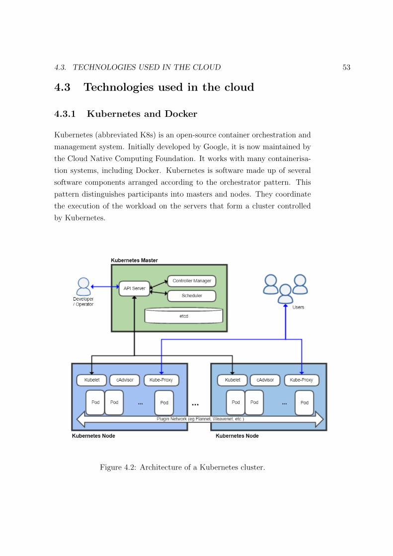
4.3. TECHNOLOGIES USED IN THE CLOUD 53
4.3 Technologies used in the cloud
4.3.1 Kubernetes and Docker
Kubernetes (abbreviated K8s) is an open-source container orchestration and
management system. Initially developed by Google, it is now maintained by
the Cloud Native Computing Foundation. It works with many containerisa-
tion systems, including Docker. Kubernetes is software made up of several
software components arranged according to the orchestrator pattern. This
pattern distinguishes participants into masters and nodes. They coordinate
the execution of the workload on the servers that form a cluster controlled
by Kubernetes.
Figure 4.2: Architecture of a Kubernetes cluster.

54 CHAPTER 4. IMPLEMENTATION
Fig. 4.2 shows the architecture of a cluster, in the case of this project
only one cluster was developed, with two worker nodes and one master node.
The pod is the resource describing the elementary unit executable on a clus-
ter node. A pod groups containers that share resources and run on the same
node. The pod abstracts network and storage in order to be easily moved and
replicated on cluster nodes, allowing strong horizontal scalability, especially
for microservice oriented applications.
Pods can be managed manually via Kubernetes APIs or more frequently via
controllers that ensure their execution is maintained [45] [46].
Docker is an open-source project that automates the deployment (delivery
or release to the customer, with associated installation and commissioning or
operation, of an application or software system typically within an enterprise
information system) of applications within software containers, providing an
additional abstraction through virtualization at the Linux operating system
level [47]. Docker uses Linux kernel resource isolation features such as cgroup
and namespace to allow independent ”containers” to coexist on the same
Linux instance, avoiding installation and maintenance.
Docker implements high-level APIs to manage containers that run processes
in isolated environments [48]. Because it uses Linux kernel functionality
(primarily cgroup and namespaces), a Docker container, unlike a virtual ma-
chine, does not include a separate operating system [49]. Instead, it uses
kernel functionality and leverages resource isolation (CPU, memory, block
I/O, network) and separate namespaces to isolate what the application can
see of the operating system. So is supported having multiple containers with
different application requirements and dependencies to run on the same host,
as long as they have the same operating system requirements.
According to industry analysis firm 451 Research, ”Docker is a tool that
can package an application and its dependencies into a virtual container that
can run on any Linux server” [49].
Using Docker to create and manage containers can simplify the creation
of distributed systems, allowing different applications or processes to work
4.3. TECHNOLOGIES USED IN THE CLOUD 55
autonomously on the same physical machine or on different virtual machines.
4.3.2 IoT managing platform - ThingsBoard
First of all ThingsBoard is presented and then some other existing platforms
specialised in managing, processing and monitoring data and devices from
the IoT are described. For example, classical databases cannot be relied upon
because we are talking about much larger data volumes.
ThingsBoard is an open-source IoT platform that enables rapid develop-
ment, management, and scaling of IoT projects. It provides an out-of-the-box
IoT cloud that enable server-side infrastructure for IoT applications, offer-
ing device management, data collection, visualization, and processing. The
platform integrates fault-tolerance, production and scalability.
With ThingsBoard, is possible to:
• Provision devices, assets and customers, and define relations between
them.
• Collect and visualize data from devices and assets.
• Analyze incoming telemetry and trigger alarms with complex event
processing.
• Control devices using remote procedure calls (RPC).
• Build work-flows based on a device life-cycle event, REST API event,
RPC request, etc.
• Design dynamic and responsive dashboards and present device or asset
telemetry and insights to your customers.
• Enable use-case specific features using customizable rule chains.
• Push device data to other systems.
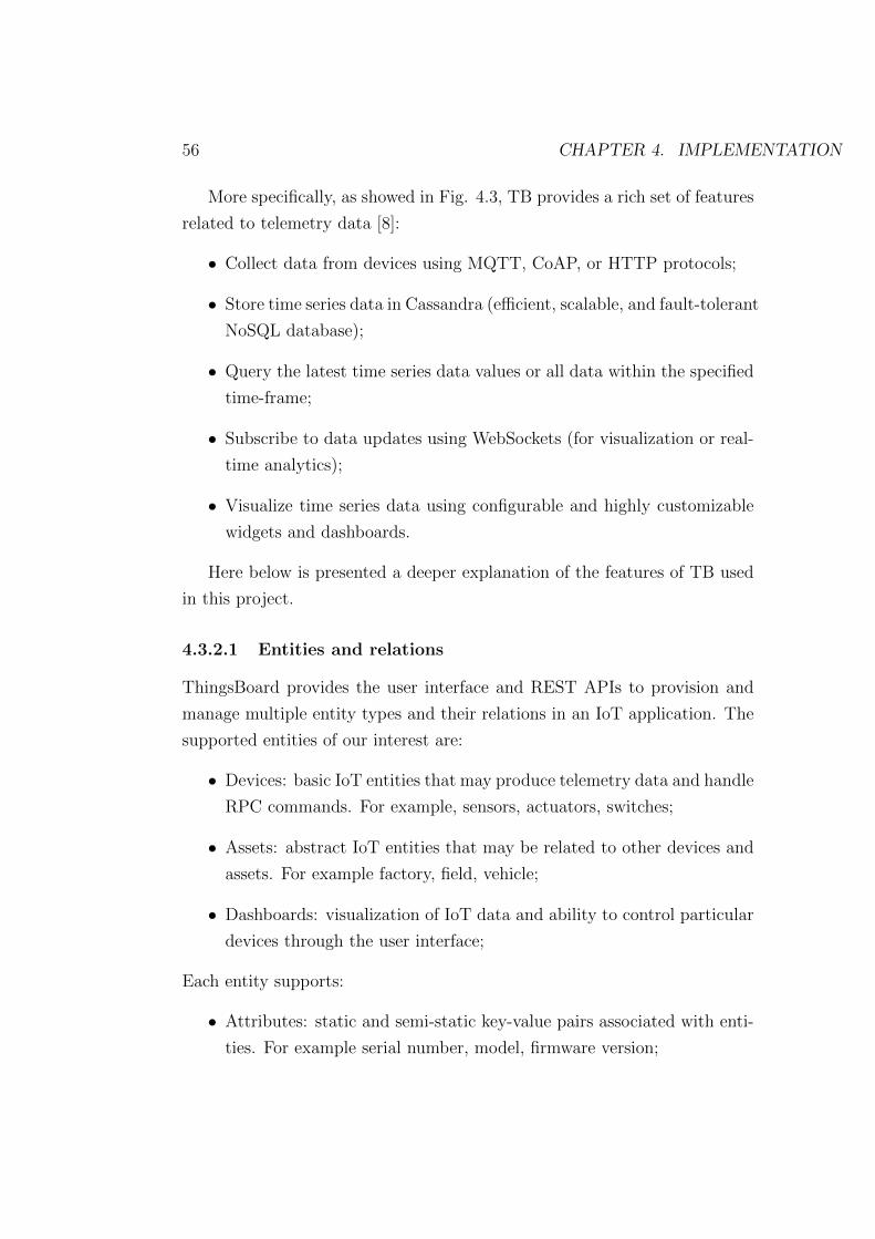
56 CHAPTER 4. IMPLEMENTATION
More specifically, as showed in Fig. 4.3, TB provides a rich set of features
related to telemetry data [8]:
• Collect data from devices using MQTT, CoAP, or HTTP protocols;
• Store time series data in Cassandra (efficient, scalable, and fault-tolerant
NoSQL database);
• Query the latest time series data values or all data within the specified
time-frame;
• Subscribe to data updates using WebSockets (for visualization or real-
time analytics);
• Visualize time series data using configurable and highly customizable
widgets and dashboards.
Here below is presented a deeper explanation of the features of TB used
in this project.
4.3.2.1 Entities and relations
ThingsBoard provides the user interface and REST APIs to provision and
manage multiple entity types and their relations in an IoT application. The
supported entities of our interest are:
• Devices: basic IoT entities that may produce telemetry data and handle
RPC commands. For example, sensors, actuators, switches;
• Assets: abstract IoT entities that may be related to other devices and
assets. For example factory, field, vehicle;
• Dashboards: visualization of IoT data and ability to control particular
devices through the user interface;
Each entity supports:
• Attributes: static and semi-static key-value pairs associated with enti-
ties. For example serial number, model, firmware version;
4.3. TECHNOLOGIES USED IN THE CLOUD 57
Figure 4.3: High-level ThingsBoard architecture overview.
• Telemetry data: time-series data points available for storage, querying
and visualization. For example temperature, humidity, battery level;
• Relations: directed connections to other entities. For example contains,
manages, owns, produces.
In our case the microgrids (Assets) contain various boards (Devices), see
Fig. 4.4.

58 CHAPTER 4. IMPLEMENTATION
Figure 4.4: ThingsBoard Assets - Devices relations in our use case [8].
4.3.2.2 Dashboards
ThingsBoard provides the ability to create and manage Dashboards. Each
Dashboard may contain plenty of widgets (e.g. Fig. 4.5) and display data
from many entities: devices, assets, etc.
4.3.2.3 Rule Engine
Rule Engine is an easy to use framework for building event-based workflows.
There are 3 main components:
• Message: any incoming event. It can be an incoming data from devices,
device life-cycle event, REST API event, RPC request, etc.
• Rule Node: a function that is executed on an incoming message. There
are many different Node types that can filter, transform or execute some
action on incoming Message.
• Rule Chain: nodes are connected with each other with relations, so the
outbound message from rule node is sent to next connected rule nodes.
Here are some common use cases that one can configure via ThingsBoard
Rule Chains:

4.3. TECHNOLOGIES USED IN THE CLOUD 59
Figure 4.5: Widget example [8].
• Data validation and modification for incoming telemetry or attributes
before saving to the database.
• Trigger actions based on device life-cycle events. For example, create
alerts if Device is Online/Offline.
• Load additional data required for processing. For example, load tem-
perature threshold value for a device that is defined in Device’s Cus-
tomer or Tenant attribute.
• Trigger REST API calls to external systems.
• Send emails when complex event occurs and use attributes of other
entities inside Email Template.
• Integrate with external pipelines like Kafka, Spark, AWS services, etc.
4.3.2.4 REST Client
The ThingsBoard REST API Client helps you interact with ThingsBoard
REST API from your Java application, with Rest Client you can program-

60 CHAPTER 4. IMPLEMENTATION
matically create assets, devices, customers, users and other entities and their
relations in ThingsBoard [8].
4.3.2.5 Others IoT platforms
Astarte Astarte is an Open Source IoT platform focused on Data man-
agement. It takes care of everything from collecting data from devices to
delivering data to end-user applications.
Ii is an Open Source IoT platform written in Elixir and it is a turnkey solu-
tion which packs in everything needed for connecting a device fleet to a set of
remote applications. It performs data modeling, automated data reduction
and real-time events.
Although Astarte’s main supported protocol is MQTT, Astarte can work
with any transport which provides a mean of authentication/authorization
and can be mapped to a key/value paradigm. Astarte can be used with
CoAP, HTTP and pretty much any protocol. And being Open Source, de-
velopers can implement their favorite protocol or wrapper, and have Astarte
work with it seamlessly.
InfluxDB InfluxDB is an open-source time series database (TSDB) de-
veloped by InfluxData. It is written in Go and optimized for fast, high-
availability storage and retrieval of time series data in fields such as oper-
ations monitoring, application metrics, Internet of Things sensor data, and
real-time analytics [50].
InfluxDB has no external dependencies and provides an SQL-like language
with built-in time-centric functions for querying a data structure composed
of measurements, series, and points. Each point consists of several key-value
pairs called the fieldset and a timestamp. When grouped together by a set
of key-value pairs called the tagset, these define a series [51].
Grafana Grafana is a multi-platform open source analytics and interactive
visualization web application. It provides charts, graphs, and alerts for the
web when connected to supported data sources.
As a visualization tool, Grafana is a popular component in monitoring stacks,

4.3. TECHNOLOGIES USED IN THE CLOUD 61
often used in combination with time series databases such as InfluxDB; mon-
itoring platforms and other data sources [52].
4.3.3 Kafka as message broker
Apache Kafka is an open-source stream-processing software platform devel-
oped by the Apache Software Foundation, written in Scala and Java. The
project aims to provide a unified, high-throughput, low-latency platform for
handling real-time data feeds. Kafka can connect to external systems (for
data import/export) via Kafka Connect and provides Kafka Streams, a Java
stream processing library. Kafka uses a binary TCP-based protocol that
is optimized for efficiency and relies on a ”message set” abstraction that
naturally groups messages together to reduce the overhead of the network
roundtrip.
Apache Kafka is based on the commit log, and it allows users to subscribe to
it and publish data to any number of systems or real-time applications [9].
Figure 4.6: Overview of Apache Kafka [9]
As showed in Fig. 4.6, Kafka stores key-value messages that come from
arbitrarily many processes called producers. The data can be partitioned into
different ”partitions” within different ”topics”. Within a partition, messages

62 CHAPTER 4. IMPLEMENTATION
are strictly ordered by their offsets (the position of a message within a par-
tition), and indexed and stored together with a timestamp. Other processes
called ”consumers” can read messages from partitions. For stream process-
ing, Kafka offers the Streams API that allows writing Java applications that
consume data from Kafka and write results back to Kafka.
Kafka runs on a cluster of one or more servers (called brokers), and the par-
titions of all topics are distributed across the cluster nodes. Additionally,
partitions are replicated to multiple brokers. This architecture allows Kafka
to deliver massive streams of messages in a fault-tolerant fashion.
4.3.3.1 Kafka Streams or Streams API
In a modern context, where speed of data processing seems to be the most
functional approach in the management of many services, Kafka Streams of-
fers itself as one of the most performing and scalable solutions. In fact, it
goes beyond a Batch data processing model, performed in the background
and at predefined intervals. It provides real-time data processing and enrich-
ment, while ensuring robustness and ease of use.
This API converts the input streams to output and produces the result;
allows for the development of stateful stream-processing applications that
are scalable, elastic, and fully fault-tolerant. The main API is a stream-
processing domain-specific language (that offers high-level operators like fil-
ter, map, grouping, windowing, aggregation, joins, and the notion of tables).
4.3.4 Node.js
Node.js programming language is also used in the cloud programming as in
the case of the edge unit, see Sec. 4.2.2.
4.3.5 OptaPlanner
OptaPlanner is an Open Source AI Constraint Solver. It solves constraint
satisfaction problems with construction heuristics and metaheuristic algo-

4.3. TECHNOLOGIES USED IN THE CLOUD 63
rithms, using multithreaded incremental solving [53].
It is a lightweight, embeddable engine which optimizes planning problems. A
planning problem has an optimal goal, based on limited resources and under
specific constraints. Optimal goals can be any number of things, such as:
maximized profits (the optimal goal results in the highest possible profit),
minimized ecological footprint (the optimal goal has the least amount of en-
vironmental impact), maximized satisfaction for employees or customers (the
optimal goal prioritizes the needs of employees or customers); the ability to
achieve these goals relies on the number of resources available, such as: the
number of people, amount of time, budget, etc.
Specific constraints related to these resources must also be taken into account,
such as the number of hours a person works, their ability to use certain ma-
chines, or compatibility between pieces of equipment.
OptaPlanner is able to solve constraint satisfaction problems efficiently
by combining optimization heuristics and metaheuristics with very efficient
score calculation.
Usually, a planning problem has at least two levels of constraints: a (nega-
tive) hard constraint that must not be broken (e.g. 1 teacher cannot teach
2 different lessons at the same time) and a (negative) soft constraint that
should not be broken if it can be avoided (e.g. teacher A does not like to
teach on Friday afternoon). Some problems have positive constraints too, a
positive soft constraint (or reward) should be fulfilled if possible (e.g. teacher
B likes to teach on Monday morning).
These constraints define the score calculation (AKA fitness function) of a
planning problem. Each solution of a planning problem can be graded with
a score. With OptaPlanner, score constraints are written in an Object Ori-
ented language, such as Java code or Drools rules. Such code is easy, flexible
and scalable.
A planning problem has a number of solutions. There are several cate-
gories of solutions:
• A possible solution is any solution, whether or not it breaks any number

64 CHAPTER 4. IMPLEMENTATION
of constraints. Planning problems tend to have an incredibly large
number of possible solutions, many of those solutions are worthless.
• A feasible solution is a solution that does not break any (negative) hard
constraints. The number of feasible solutions tends to be relative to the
number of possible solutions, sometimes there are no feasible solutions
(every feasible solution is a possible solution).
• An optimal solution is a solution with the highest score. Planning
problems tend to have 1 or a few optimal solutions. There is always
at least 1 optimal solution, even in the case that there are no feasible
solutions and the optimal solution is not feasible.
• The best solution found is the solution with the highest score found by
an implementation in a given amount of time. The best solution found
is likely to be feasible and, given enough time, it’s an optimal solution.
Counterintuitively, the number of possible solutions is huge (if calculated
correctly), even with a small dataset. As there is no silver bullet to find the
optimal solution, any implementation is forced to evaluate at least a subset
of all those possible solutions.
OptaPlanner supports several optimization algorithms to efficiently wade
through that incredibly large number of possible solutions. Depending on
the use case, some optimization algorithms perform better than others, but
it’s impossible to tell in advance. With OptaPlanner, it is easy to switch the
optimization algorithm, by changing the solver configuration in a few lines
of XML or code [10].
The Fig. 4.7 shows the solving process: a construction heuristic builds
a pretty good initial solution in a finite length of time, its solution isn’t
always feasible but it finds it fast, and metaheuristics can finish the job. The
algorithms used by default are:
• First Fit regarding the Construction Heuristics phase: the First Fit
algorithm cycles through all the planning entities (in default order),

4.4. ACTUAL SYSTEM ARCHITECTURE 65
initializing one planning entity at a time, it assigns the planning en-
tity to the best available planning value, taking the already initialized
planning entities into account. It terminates when all planning entities
have been initialized and it never changes a planning entity after it has
been assigned. A construction heuristics terminate automatically, so
there’s usually no need to configure a Termination on the construction
heuristic phase specifically.
• Late Acceptance (Meta Heuristic) for the Local Search phase: heuris-
tics are often problem-dependent (an heuristic is defined for a given
problem), metaheuristics are problem-independent techniques that can
be applied to a broad range of problems.
Local Search starts from an initial solution and evolves that single so-
lution into a mostly better and better solution. It uses a single search
path of solutions, not a search tree. At each solution in this path it
evaluates a number of moves on the solution and applies the most suit-
able move to take the step to the next solution. It does that for a high
number of iterations until it’s terminated (usually because its time has
run out).
Late Acceptance (also known as Late Acceptance Hill Climbing) also
evaluates only a few moves per step. A move is accepted if does not
decrease the score, or if it leads to a score that is at least the late score
(which is the winning score of a fixed number of steps ago)[10].
4.4 Actual system architecture
The MAPE-K (Monitor-Analyze-Plan-Execute over a shared Knowledge)
loop is the most influential reference control model for autonomic and self-
adaptive systems. Here in Fig. 4.8 is presented how this can be applied to
our system:
• Monitoring: pushing data from edge-devices to TB in the cloud with
the simulator.

66 CHAPTER 4. IMPLEMENTATION
Figure 4.7: OptaPlanner solving process. [10]
• Analyzing: pre-processing with Kafka Stream aggregator together with
python consumer.
• Planning: Algorithms caller and OptaPlanner optimizer.
• Executing: Algorithm caller sends instructions to edge units.
• Shared Knowledge: Thingsboard stores the values and could implement
machine learning on data to pre-plan better actions.
The Fig. 4.9 shows the final software architecture, after choosing the
technologies for the components and the types of interaction between them.
The first component to come into play is the ThingsBoard REST Client that
has the duty to create the elements representing our case in the abstract (De-
vices as boards, Assets as microgrids and Dashboards) within ThingsBoard;
once inserted and obtained the access credentials, it is the turn of the data
simulator that generates consumption and production values (following pat-
terns according to the prosumer typology, see 3.3.2) for real-time data and

4.4. ACTUAL SYSTEM ARCHITECTURE 67
Figure 4.8: MAPE-K loop in the actual system architecture.
the data of future consumption, while inferring (through ML) the data on
future production.
When ThingsBoard receives the data from the devices, it forwards them to
the Kafka broker, to which an application is connected that, intercepting
the stream of timeseries, aggregates them according to the device and the
microgrid to which it belongs.
To this out-topic of Kafka is subscribed a consumer that, first of all, publishes
on TB the aggregated real-time data for production and consumption of each
microgrid (so that we can observe the trend in the dashboards) and, after
that, depending on the chosen strategy decides whether to use the algorithms
for the optimization of energy scheduling in OptaPlanner and communicate
the decisions taken on the batteries to the boards via RPC or whether to
communicate directly the values of import and export to ResultsTracker that
will store them on CSV files.

68 CHAPTER 4. IMPLEMENTATION
Figure 4.9: Actual system architecture with used technologies.
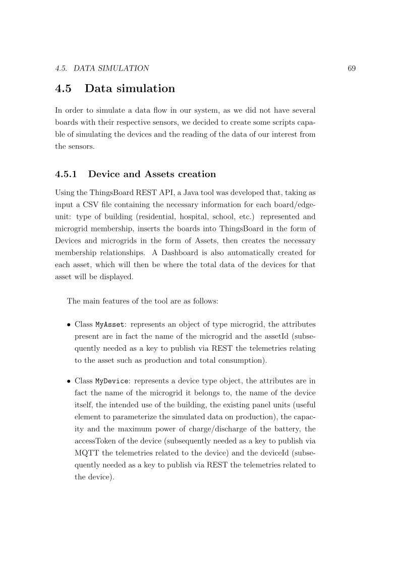
4.5. DATA SIMULATION 69
4.5 Data simulation
In order to simulate a data flow in our system, as we did not have several
boards with their respective sensors, we decided to create some scripts capa-
ble of simulating the devices and the reading of the data of our interest from
the sensors.
4.5.1 Device and Assets creation
Using the ThingsBoard REST API, a Java tool was developed that, taking as
input a CSV file containing the necessary information for each board/edge-
unit: type of building (residential, hospital, school, etc.) represented and
microgrid membership, inserts the boards into ThingsBoard in the form of
Devices and microgrids in the form of Assets, then creates the necessary
membership relationships. A Dashboard is also automatically created for
each asset, which will then be where the total data of the devices for that
asset will be displayed.
The main features of the tool are as follows:
• Class MyAsset: represents an object of type microgrid, the attributes
present are in fact the name of the microgrid and the assetId (subse-
quently needed as a key to publish via REST the telemetries relating
to the asset such as production and total consumption).
• Class MyDevice: represents a device type object, the attributes are in
fact the name of the microgrid it belongs to, the name of the device
itself, the intended use of the building, the existing panel units (useful
element to parameterize the simulated data on production), the capac-
ity and the maximum power of charge/discharge of the battery, the
accessToken of the device (subsequently needed as a key to publish via
MQTT the telemetries related to the device) and the deviceId (subse-
quently needed as a key to publish via REST the telemetries related to
the device).

70 CHAPTER 4. IMPLEMENTATION
• Class ThingsboardElementsCreator: first of all the CSV file contain-
ing the characteristics of the desired boards is read, after which the
corresponding Devices are created on Thingsboard, together with the
microgrids that are created in the form of Assets, through the REST
client; for each Device at the creation the accessToken and the deviceId
are assigned, while for the Assets only the assetId. Then the relation-
ships between Devices and Assets are established so that a microgrid
contains the correct boards and finally all the information on Device
and Asset (in particular the credentials) are saved in CSV files to be
used later.
• Class ThingsboardDashboardCreator: after reading the asset char-
acteristics (microgrid name and assetId) from the CSV file created as
output by ThingsboardElementsCreator, this class is responsible for
publishing on Thingsboard a dashboard for each of the assets using a
given JSON format dashboard template and modifying the attributes
of this JSON for each assets/microgrid.
4.5.2 Consumption and production creation
The script that takes care of this functionality is in JS format and is laid out
using NodeJS. To start it reads the content of the two CSV files produced
in the previous phase (devices and assets) through the Node module ”fs”,
that is responsible for all the asynchronous or synchronous I/O operations;
at the success of the operation it reads the content of the CSV file containing
the mean and variance for the production and consumption patterns; these
data are then used at the time of the creation of an MQTT client for each
board/edge-unit as input for the simulation of data (generating a random
number normally distributed) consistent with the building typology.
For the creation of an MQTT client, able to send telemetry to ThingsBoard
via MQTT, the accessToken of the device is required; when the connection is
successful the consumption and production data are simulated (generating a
random number following the normal distribution). Moreover, if the chosen
strategy is BAU, the local logic for the energy balance will be applied, as

4.6. ML FOR INFERENCE OF PRODUCTION DATA 71
seen in the previous section and illustrated in the algorithm 1; if the strategy
is global, no pre-computation will be done in the board before sending the
telemetries to ThingsBoard via MQTT.
A further function of the MQTT client used in this case (except with the BAU
strategy) is the ability to receive RPCs (Remote Procedure Calls): the client,
immediately after the connection registers to receive messages and defines
the actions to be performed following a given communication, in our case the
body of the message will contain how much to vary (charge/discharge) the
state of battery charge in the next time step.
4.6 ML for inference of production data
With regard to the PV panel production forecasts, introduced in the pre-
viously mentioned tool for simulation, an ML model (4-layer bi-directional
LSTM [38]) already trained for inference was used, while for consumption
forecasts the patterns of the respective prosumers are used. The input of the
inference is the production data of the previous 15 minutes with a granularity
of 30 seconds (so 30 data-points), the same for the output produced.
The Python support file inference.py uses the Tensorflow module to load the
model (this can be done once) while the simulator invokes a specific infer-
ence function (the loaded model predicts the data based on the input) at the
beginning of each time step (5 minutes), in order to obtain the prediction
information for time step +2 to be attached to the following telemetry.
4.7 ThingsBoard telemetries collection and
processing
When receiving telemetries, Thingsboard follows the so-called ”Root rule
chain”: the basic rule chain in which all messages arrive. As shown in Fig.
4.10, telemetries once saved are forwarded to Kafka broker as stream with
the predefined topic, simply by adding a node and configuration to the rule
chain.

72 CHAPTER 4. IMPLEMENTATION
Figure 4.10: Root rule chain forwarding to Kafka stream.
4.8 Kafka stream aggregator application
A Maven application was deployed in the cloud to manage the stream of
telemetries. Kafka broker receives the messages for a certain topic (in our
case we record the stream for the same topic outgoing from ThingsBoard).
The application must then first deserialize the message, save the content as
an object, aggregate the data in the chosen range, reserialize the output and
publish it in the out-topic.
In detail, the input is given by each telemetry coming from a device, with
the following attributes: microgridID, deviceID, consumption, production,
energyImport, energyExport, predicted consumption, predicted production,
battery capacity, battery state of charge, charging and discharging limit. If
the chosen strategy is BAU all these attributes will have a value because
they are the result of a pre-computation local to the board (except for pre-
dicted consumption and production that are not used because in this case we
are not interested in forecasting because prediction is used to decide on the
scheduling of prosumer batteries based on the exchanges they have to make
within the microgrid, but with the local BAU strategy each prosumer decides
autonomously), vice versa for the other strategies energyImport and energy-
Export will not be initialized because we will refer directly to the global ones
of the microgrid once the scheduling problem is optimized.
Regarding aggregation, it is performed according to the key that is declared,
in this case the key defined was (microgridID, deviceID); each telemetry pub-

4.8. KAFKA STREAM AGGREGATOR APPLICATION 73
lished as output of the stream in the cloud is therefore the aggregation by
device in a 5-minute interval with also the aggregation by microgrid (see the
following JSON schema that respects what is specified in the tables 3.2 3.3),
consequently the aggregation by microgrid could be redundant.
Listing 4.1: JSON schema of the message for aggregated data about a device
” type ” : ” ob j e c t ” ,
” p r o p e r t i e s ” : {” microgr idID ” : {” type ” : ” s t r i n g ”} ,
” deviceID ” : {” type ” : ” s t r i n g ”} ,
” count ” : {” type ” : ”number ”} ,
”sumConsumption ” : {” type ” : ”number ”} ,
” sumProduction ” : {” type ” : ”number ”} ,
” sumPredictedConsumption ” : {” type ” : ”number ”} ,
” sumPredictedProduction ” : {” type ” : ”number ”} ,
” sumEnergyImport ” : {” type ” : ”number ”} ,
”sumEnergyExport ” : {” type ” : ”number ”} ,
” capac i ty ” : {” type ” : ”number ”} ,
” sumStateOfEnergy ” : {” type ” : ”number ”} ,
” avgStateOfEnergy ” : {” type ” : ”number ”} ,
” charg ingLimit ” : {” type ” : ”number ”} ,
” d i s charg ingL imi t ” : {” type ” : ”number ”} ,
” microgr idAggregator ” :
{ ” type ” : ” ob j e c t ” ,
” p r o p e r t i e s ” : {” microgr idID ” : {” type ” : ” s t r i n g ”} ,
” count ” : {” type ” : ”number ”} ,
”sumConsumption ” : {” type ” : ”number ”} ,
” sumProduction ” : {” type ” : ”number ”} ,
” sumPredictedConsumption ” : {” type ” : ”number ”} ,
” sumPredictedProduction ” : {” type ” : ”number ”} ,
” sumEnergyImport ” : {” type ” : ”number ”} ,
”sumEnergyExport ” : {” type ” : ”number”}

74 CHAPTER 4. IMPLEMENTATION
}}
}
It should be noted finally that in order to aggregate all parameters, except
for the state of charge of the battery where a mathematical average of the
values is made, the data are summed.
4.9 Consumer of the aggregated data
The application that consumes the data from the topic containing the aggre-
gated values has been written in Python (see Python Consumer in Fig.4.9).
Once the message is received, it checks that it respects the default JSON
schema Lst. 4.1, if not, the content is ignored. If the schema is compliant,
the content is parsed and processed:
1. The ”properties” of the ”microgridAggregator” element are sent with
the ThingsBoard REST API to the microgrid assets, to be visualized
in a dashboard (see Fig. 4.11), as they represent the aggregation of
all the telemetries received for the devices of that microgrid. Since, as
explained above, this data is redundant for all aggregated devices, it is
sent to ThingsBoard only the first time, to identify the uniqueness of
the data the microgridID (formed by the ID of the microgrid and the
time-step identifier) is taken into account.
2. (a) In the case where the chosen strategy is BAU type, without hav-
ing to turn to the optimisation algorithm, the data aggregated
by microgrid on import and export are directly sent to the Node
service created ResultsTracker which, for the purposes of perfor-
mance evaluation and comparison, keeps them updated by writing
them in a CSV file.
(b) If the chosen strategy is a global one (minimum cost or mini-
mum exchange), all the aggregated data of the devices present
in the same microgrid are collected and sent to the supporting
4.10. SUPPORT WEB SERVICE ALGORITHMCALLER 75
Figure 4.11: Dashboard of a microgrid showing aggregated data of its devicesabout the last 10 minutes.
Node service AlgorithmCaller so that the latter can manage asyn-
chronously the request to the algorithm in the OptaPlanner ap-
plication.
4.10 Support web service AlgorithmCaller
This web service exposes a number of APIs, in particular the ability to call the
optimisation algorithm on OptaPlanner given the aggregated edge-devices
data as input. The endpoint for the request is ’/addsolve’ and the parameters
in the body accepted are the list of prosumer data and the type of strategy
76 CHAPTER 4. IMPLEMENTATION
to be used for the algorithm, all in JSON format; once the request is received
the service makes the solve enquiry to OptaPlanner sending it also the device
data and, at regular intervals, checks if a solution has been found or not:
in case of positive outcome the optimised energy scheduling is obtained,
otherwise it is tried again after a certain time.
When the solution is found:
1. the results are sent (import and export of the microgrid) to the Result-
sTracker service which will update its data;
2. the settings points on how to manage the prosumer’s devices (e.g. how
to charge/discharge the battery) are sent to the to the prosumer’s local
controller, via ThingsBoard RPC.
4.11 Energy scheduling optimizer
In our case we have two planning problems that differ in the goal (minimising
the total cost incurred by the microgrid or minimising the amount of energy
exchanged with the main grid) but have constraints in common (see 3.5.3.1
regarding the energy balance and battery scheduling).
A Maven project has been therefore created in Java using OptaPlanner
to solve these planning problems.
First, the classes representing the problem domain were defined (see Fig.
4.12):
• Prosumer: is considered a PlanningEntity, i.e. it varies during the res-
olution of the problem. Its static attributes are: id of the microgrid
it belongs to, id of the device itself, expected consumption and pro-
duction, battery capacity and charge/discharge limits, battery charge
status; while the PlanningVariable is the battery scheduling in the next
time-step (charge/discharge and quantity). The energy balance of a
prosumer is given by the difference between expected production and
consumption to which the battery scheduling is added.

4.11. ENERGY SCHEDULING OPTIMIZER 77
Figure 4.12: Class diagram of the domain model.
• Microgrid: is considered a PlanningEntity, the attribute that varies is
the energy exchange while the only other attribute is the identifier of
the microgrid itself. A microgrid can contain one or more prosumers.
• Solution: in this class of type PlanningSolution the attributes are the
list of microgrids and the list of prosumers as PlanningEntityCollection
and the relative score. Here the value ranges for the PlanningVariables
of the PlanningEntities are also specified, i.e. the possible values for
the prosumers’ battery charge/discharge and the amount of energy ex-
changed between the microgrids and the main grid.
After that, for the ”Entity” classes (Microgrid.java and Prosumer.java)
repositories were created with Panache Quarkus to give persistence.
For each of the three classes listed above, the possibility of access via
REST API to the resource has also been created; the Solution.java class
is however the only one which, in addition to the simple REST methods for
adding or removing, implements further endpoints such as launching a search
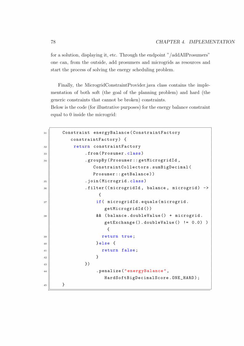
78 CHAPTER 4. IMPLEMENTATION
for a solution, displaying it, etc. Through the endpoint ”/addAllProsumers”
one can, from the outside, add prosumers and microgrids as resources and
start the process of solving the energy scheduling problem.
Finally, the MicrogridConstraintProvider.java class contains the imple-
mentation of both soft (the goal of the planning problem) and hard (the
generic constraints that cannot be broken) constraints.
Below is the code (for illustrative purposes) for the energy balance constraint
equal to 0 inside the microgrid:
31 Constraint energyBalance(ConstraintFactory
constraintFactory) {
32 return constraintFactory
33 .from(Prosumer.class)
34 .groupBy(Prosumer :: getMicrogridId ,
ConstraintCollectors.sumBigDecimal(
Prosumer :: getBalance))
35 .join(Microgrid.class)
36 .filter (( microgridId , balance , microgrid) ->
{
37 if( microgridId.equals(microgrid.
getMicrogridId ())
38 && (balance.doubleValue () + microgrid.
getExchange ().doubleValue () != 0.0) )
{
39 return true;
40 }else {
41 return false;
42 }
43 })
44 .penalize("energyBalance",
HardSoftBigDecimalScore.ONE_HARD);
45 }

4.12. SUPPORT WEB SERVICE RESULTSTRACKER 79
As it can be seen, the sum of the energy balances of the prosumers is cal-
culated respecting the constraint stated in equation 3.3 (it is not obligatory
for each prosumer to be 0 as in the end the overall positive or negative bal-
ance of the microgrid is compensated by the import/export of the microgrid
itself) and is then compared with the energy exchange value of the microgrid
with the main grid, this value must compensate for the balance in order to
reach 0; if it is not 0, the HardScore of the solution is penalised by 1 point,
going negative. In our use case all solutions with a HardScore equal to 0 are
considered feasible solutions, but they are not always optimal.
In order to evaluate which solution is better than another among the fea-
sible ones, the SoftScore is analysed, as an example the code of the goal for
the minimum energy exchange strategy is shown:
46 Constraint minEnergyExchange(ConstraintFactory
constraintFactory) {
47 return constraintFactory
48 .from(Microgrid.class)
49 .penalizeBigDecimal("minEnergyExchange",
HardSoftBigDecimalScore.ONE_SOFT ,
50 Microgrid :: getAbsValExchange );
51 }
In this case, as it can be seen, for each microgrid the amount of energy
exchanged (import or export) is checked and the SoftScore is penalised by
that value; the optimality in this case would be that all the microgrids had
an exchange of 0.
4.12 Support web service ResultsTracker
This service has been created in order to have an automated record of the
results obtained with both the local BAU scheduling and the global ones, so
that they can be compared. Its API exposes an endpoint for each strategy

80 CHAPTER 4. IMPLEMENTATION
and when a scheduling solution is received it is temporarily saved in the
corresponding support array (one for each strategy). Every 10 seconds it
updates the content of the CSV files (one for each strategy) with the import
and export values of the supporting arrays.

Chapter 5
Evaluation
This chapter presents the results of the final phase of the project’s perfor-
mance evaluation. First of all, an environment useful only for testing was
recreated, then different scenarios of microgrid composition were created, and
finally the parameters (briefly introduced in Sect. 3.6), different for each of
the strategies according to the objective, were evaluated.
5.1 Scenarios
Three scenarios have been created for testing:
• 2 microgrids with only residential prosumers: with the characteristics
shown in Tab. 5.1;
• 2 microgrids with only commercial prosumers: with the characteristics
shown in Tab. 5.2;
• 2 microgrids with residential and commercial prosumers together: with
the characteristics shown in Tab. 5.3.
We remind that the optimisation strategies are addressed to the single mi-
crogrid, foreseeing energy exchanges only between prosumers within the same
microgrid and not between those belonging to different microgrids. Outside
the cluster there are exchanges only with the DSO.
81

82 CHAPTER 5. EVALUATION
MicrogridID
Device ID BuildingType
PanelsUnits
BatteryCapacity
ChargingLimit
DischargingLimit
Microgrid-1 Device-1 Residential 1 50 0.4 0.4Microgrid-1 Device-2 Residential 1 50 0.4 0.4Microgrid-1 Device-3 Residential 1 50 0.4 0.4Microgrid-2 Device-4 Residential 1 50 0.4 0.4Microgrid-2 Device-5 Residential 1 50 0.4 0.4Microgrid-2 Device-6 Residential 1 50 0.4 0.4
Table 5.1: Microgrids testing scenario 1.
MicrogridID
Device ID BuildingType
PanelsUnits
BatteryCapacity
ChargingLimit
DischargingLimit
Microgrid-1 Device-1 Hotel 70 100 0.4 0.4Microgrid-1 Device-2 Supermarket 70 100 0.4 0.4Microgrid-1 Device-3 Mall 70 100 0.4 0.4Microgrid-2 Device-4 Hospital 230 100 0.4 0.4Microgrid-2 Device-5 School 120 100 0.4 0.4Microgrid-2 Device-6 Supermarket 70 100 0.4 0.4
Table 5.2: Microgrids testing scenario 2.
With regard to the prices of energy imported and exported by the micro-
grid, in our use case we have referred to the Eurostat 2020 statistics and the
Eurostat 2020 statistics [54] and to [55].
The EU-27 average price in the first semester of 2020, a weighted average us-
ing the most recent (2020) data for electricity consumption by non-household
consumers (given that the microgrid is considered a single entity with an
overall consumption level higher than residential), was 0.1254 €/kWh (in
our case approximated to 0.13 EUR per kWh). As far as energy fed into the
grid is concerned, this is valued on average at 0.09-0.10 €/kWh.

5.2. TESTING DATAFLOW 83
MicrogridID
Device ID BuildingType
PanelsUnits
BatteryCapacity
ChargingLimit
DischargingLimit
Microgrid-1 Device-1 Residential 1 50 0.4 0.4Microgrid-1 Device-2 Residential 1 50 0.4 0.4Microgrid-1 Device-3 Mall 70 100 0.4 0.4Microgrid-2 Device-4 Residential 1 50 0.4 0.4Microgrid-2 Device-5 School 120 100 0.4 0.4Microgrid-2 Device-6 Supermarket 70 100 0.4 0.4
Table 5.3: Microgrids testing scenario 3.
5.2 Testing dataflow
In order to obtain comparable results in the strategies, we decided to create
a standard input for each scenario in order to have the same production and
consumption values for each prosumer.
For the set of devices indicated in each of the three different scenarios, the
simulator (4.5.2) was then started for a period of one hour, during which
the BAU strategy (local decisions to each device) was performed. After the
aggregation phase by the Kafka Stream, via the Python consumers, from the
aggregated telemetries obtained:
• the summed import and export values for each microgrid were stored
by the ResultsTracker (in an external CSV file);
• the consumption and production values were forwarded to the energy
scheduler in OptaPlanner to obtain the import and export values also
in the two global strategies, also in this case the results were sent to
the ResultsTracker.
It should be noted that, running everything at the same time, in the
case of the BAU strategy the SoE battery was changed automatically by
the device, while with the global strategies instead of changing it with the
RPC (which would have affected the changes made in real-time by the local
strategy) it was changed in the AlgorithmCaller in the next time-step for
each device.

84 CHAPTER 5. EVALUATION
5.3 Results
This section presents the results obtained in the three scenarios, comparing
the different strategies.
The outcomes show that just applying an optimisation strategy to a cluster
of prosumers is not enough. It is necessary to evaluate the composition of a
microgrid in such a way as to have deficits and surpluses roughly balanced
between them, which can be done by comparing past production and con-
sumption data for each prosumer, the more balanced they are the better the
optimisation will be.
It is also good practice to assess the best battery capacity for each require-
ment, e.g. if a minimum exchange strategy is to be pursued it is good to
have a high storage capacity.
5.3.1 Residential scenario
Regarding the results in the residential scenario (see Tab. 5.4) we can note
that the results are not optimized.
This is due to the fact that, as we can already see in the BAU strategy, there
is in general no energy surplus in either of the two microgrids.
In the two strategies, initially the deficits of the single prosumers are compen-
sated with the batteries of all the others that have charge available but, since
there is never an energy surplus, the batteries are not given the possibility
to recharge and these, remaining at the minimum level, have no possibility
to exchange energy.
Each prosumer can therefore rely solely on the main grid to import energy
and respect the energy balance.
5.3.2 Commercial scenario
Regarding the results in the business scenario (see Tab. 5.5) we can note
that:
• With the minimum exchange strategy, an overall reduction in exchanged
power was effectively achieved, for both microgrids, compared to the
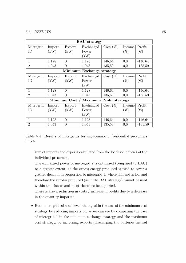
5.3. RESULTS 85
BAU strategy
MicrogridID
Import(kW)
Export(kW)
ExchangedPower(kW)
Cost (€) Income(€)
Profit(€)
1 1.128 0 1.128 146,64 0,0 -146,642 1.043 0 1.043 135,59 0,0 -135,59
Minimum Exchange strategy
MicrogridID
Import(kW)
Export(kW)
ExchangedPower(kW)
Cost (€) Income(€)
Profit(€)
1 1.128 0 1.128 146,64 0,0 -146,642 1.043 0 1.043 135,59 0,0 -135,59
Minimum Cost / Maximum Profit strategy
MicrogridID
Import(kW)
Export(kW)
ExchangedPower(kW)
Cost (€) Income(€)
Profit(€)
1 1.128 0 1.128 146,64 0,0 -146,642 1.043 0 1.043 135,59 0,0 -135,59
Table 5.4: Results of microgrids testing scenario 1 (residential prosumersonly).
sum of imports and exports calculated from the localised policies of the
individual prosumers.
The exchanged power of microgrid 2 is optimised (compared to BAU)
to a greater extent, as the excess energy produced is used to cover a
greater demand in proportion to microgrid 1, where demand is low and
therefore the surplus produced (as in the BAU strategy) cannot be used
within the cluster and must therefore be exported.
There is also a reduction in costs / increase in profits due to a decrease
in the quantity imported.
• Both microgrids also achieved their goal in the case of the minimum cost
strategy by reducing imports or, as we can see by comparing the case
of microgrid 1 in the minimum exchange strategy and the maximum
cost strategy, by increasing exports (discharging the batteries instead

86 CHAPTER 5. EVALUATION
of storing the energy).
BAU strategy
MicrogridID
Import(kW)
Export(kW)
ExchangedPower(kW)
Cost (€) Income(€)
Profit(€)
1 277 20.559 20.836 36,01 2.055,90 2.019,802 15.617 13.133 28.750 2.030,21 1.313,30 -716,91
Minimum Exchange strategy
MicrogridID
Import(kW)
Export(kW)
ExchangedPower(kW)
Cost (€) Income(€)
Profit(€)
1 0 20.821 20.821 0,0 2.082,10 2.082,102 4.516,5 979,5 5.496 587,14 97,95 -489,19
Minimum Cost / Maximum Profit strategy
MicrogridID
Import(kW)
Export(kW)
ExchangedPower(kW)
Cost (€) Income(€)
Profit(€)
1 0 20.890 20.890 0,0 2.089,90 2.089,902 3.737,5 1.302,5 5.040 485,87 130,25 -355,62
Table 5.5: Results of microgrids testing scenario 2 (commercial prosumersonly).
5.3.3 Mixed scenario
Regarding the results in the scenario with both residential and commercial
prosumers (see Tab. 5.6) we can note that:
• For the minimum exchange strategy, in both microgrids, the overall
exchanged power corresponds more or less to the balance that would
be obtained in the BAU strategy by subtracting the energy deficit to the
surplus (by acting with the BAU locally to each device without having
a global overview, it is however impossible to achieve this objective if
not with a global strategy such as minimum exchange); profits are also
increased.

5.3. RESULTS 87
• As regards profit maximisation, we can say that, again, balancing im-
port (low) and export (high) and selling the stored energy of the bat-
teries (thus not keeping them always at a high level of charge) resulted
in a good increase in profits, but increased exchanged power.
BAU strategy
MicrogridID
Import(kW)
Export(kW)
ExchangedPower(kW)
Cost (€) Income(€)
Profit(€)
1 1.010 2.625 3.635 131,3 262,50 131,202 929 13.219 14.148 120,77 1.321,90 1201,13
Minimum Exchange strategy
MicrogridID
Import(kW)
Export(kW)
ExchangedPower(kW)
Cost (€) Income(€)
Profit(€)
1 0 1.682,5 1.682,5 0,0 168,25 168,252 0 12.271,5 12.271,5 0,0 1.227,15 1.227,15
Minimum Cost / Maximum Profit strategy
MicrogridID
Import(kW)
Export(kW)
ExchangedPower(kW)
Cost (€) Income(€)
Profit(€)
1 13 1.700,5 1.713,5 1,69 170,05 168,812 0 12.321 12.321 0,0 1232,10 1232,10
Table 5.6: Results of microgrids testing scenario 3 (mixed types of pro-sumers).
Moreover, only for this scenario, the graphs in Fig. 5.1 and 5.1 show
the aggregated production and consumption values for Microgrid 1 in the
considered interval of 1 hour and the exchange values (positive in case of
export and negative in case of import) that the microgrid would have if the
prosumers did not have any kind of storage device (BES).
The Tab. 5.7 presents the import and export values (and respective costs)
of the two microgrids analysed, in the case where prosumers can compensate
each other for individual surpluses and deficits but do not have a storage

88 CHAPTER 5. EVALUATION
Figure 5.1: Aggregated values for Microgrid 1 in the observed interval of 1hour.
Figure 5.2: Aggregated values for Microgrid 2 in the observed interval of 1hour.

5.4. TESTING OF DIFFERENT ALGORITHMS CONFIGURATIONS 89
device (BES).
Analysing the values and comparing them with those in Tab. 5.6 it emerges
that:
• Microgrid 1: the total exchanged power is higher than for the two
global optimisation strategies but still lower (therefore better to give
autonomy to the grid) than for the local non-cooperation prosumer
(BAU) strategy, the total profit is lower than for all three previous
strategies.
• Microgrid 2: the total exchanged power is higher than that obtained
with the minimum exchange algorithm but lower than the value that
would be obtained with the local optimisation or the minimum cost
strategy; the same result is obtained with the total profit, which is
worse only than the amount obtained with the profit maximisation
strategy.
No battery usage
MicrogridID
Import(kW)
Export(kW)
ExchangedPower(kW)
Cost (€) Income(€)
Profit(€)
1 354,5 1.727 2.081,5 46,09 172,70 126,612 0 12.295,5 12.295,5 0 1.229,55 1.229,55
Table 5.7: Results of microgrids testing scenario 3 without BES.
5.4 Testing of different algorithms configura-
tions
For both global strategies the default optimizing algorithms are applied (first
fit for the construction heuristics phase and late acceptance for the local
search phase), as after some tests it was noticed that the score obtained (or
the number of moves to obtain it) did not improve with the other alternatives.

90 CHAPTER 5. EVALUATION
These algorithms are also influenced by the resolution times and termination
conditions imposed in the configuration phase:
• solver.termination.spent-limit : with this element we configure the max-
imum processing time for the algorithm, for the test a time limit of 2
minutes was used, after having proven that even with 5 minutes it gave
the same result and did not give a better score.
• solver.termination.best-score-limit : this element imposes an early ter-
mination on the algorithm in case of premature achievement of the
goal (e.g. score 0hard/0soft means getting 0 hard and soft constraints
broken, which is usually the optimal solution). However, not all strate-
gies benefit from the inclusion of this condition (which usually avoids
unnecessary computation in the server), such as cost minimisation or
profit maximisation because it ends the solving process as soon as it
has a positive score and, in the case of energy exports, that score can
be improved because selling energy gives a positive score with a reward.

Chapter 6
Conclusions and Future Works
The aim of this thesis was to create a hardware and software architecture
for monitoring and managing energy resources in microgrids, optimising the
exchange of energy resources between the various ”prosumers” that make up
the microgrid.
The result was an edge-cloud structure, with initial processing of data near
the place where it is generated (prosumer) and subsequent management in
the cloud for resources shared with other edge nodes.
From the analysis of the results obtained by applying this optimisation to
real scenarios, it is emerged that the heterogeneity of the types of prosumers
that constitute a microgrid (i.e. their production and consumption patterns)
and the type of storage chosen have a great impact on the quality of energy
scheduling, regardless of the hardware and software technologies used.
Despite this, both strategies implemented have good optimizations (min-
imum exchange and minimum cost) compared to traditional (BAU) or a
microgrid whose prosumers have no energy storage devices for the extra-
production.
6.1 Future Work
For the extension of the work presented in this master thesis, the first step
could be to introduce the possibility for prosumers within a certain geograph-
91

92 CHAPTER 6. CONCLUSIONS AND FUTURE WORKS
ical radius to switch the microgrid they belong to in order to optimise the
overall performance (as shown in the evaluation, optimisation was more ef-
fective if import and export were balanced with each other) or, using ML
based clustering with graph networks, to identify prosumers with optimal
exchange possibilities.
Furthermore, in combination with the ML model used for inference re-
garding the energy production of PVs, we could add a model that predicts
consumption for different profiles of prosumers (commercial or residential
and, in the case of residential, also have as data the number of occupants
etc.) based on a larger training dataset (so that, for example, the season of
the year or the day of the week is also taken into account).
Finally, it would be very useful to add an internal energy market within
the microgrid with prices that vary according to the supply and demand
of individual prosumers; in connection with this, the demand of prosumers
could be dynamically managed by shifting it from peak to off-load periods
for non-essential energy consumption (e.g. recharging an electric vehicle).

Bibliography
[1] Energy atlas 2018 – facts and figures about renewables in europe.
https://gef.eu/wp-content/uploads/2018/04/energyatlas2018_
facts-and-figures-renewables-europe.pdf. visited 10-Feb-2021.
[2] Peter Vaessen. Will microgrids become the dominant electric power
supply source of the future? https://blogs.dnvgl.com/energy/
will-microgrids-become-the-dominant-electric-power-supply-\
\source-of-the-future. visited 15-Feb-2021.
[3] Mehdi Jalali, Kazem Zare, and Heresh Seyedi. Strategic decision-making
of distribution network operator with multi-microgrids considering de-
mand response program. Energy, 141:1059–1071, 2017.
[4] Wenbo Shi, Na Li, Chi-Cheng Chu, and Rajit Gadh. Real-time energy
management in microgrids. IEEE Transactions on Smart Grid, 8, 08
2015.
[5] Siemens - microgrid control. https://new.siemens.com/global/
en/products/energy/energy-automation-and-smart-grid/
microgrid/sicam-microgrid-controller.html. visited 12-Feb-
2021.
[6] Siemens - spectrum power™ mgms. https://new.siemens.com/
global/en/products/energy/energy-automation-and-smart-\
\grid/microgrid/spectrum-power-mgms.html. visited 12-Feb-2021.
[7] Kyriaki Antoniadou-Plytaria. Optimal energy scheduling of grid-
93

94 BIBLIOGRAPHY
connected microgrids with battery energy storage. Master’s thesis,
Chalmers University of Technology, 2020.
[8] Thingsboard user guide. https://thingsboard.io/docs/user-guide.
visited 18-Feb-2021.
[9] Overview of apache kafka. https://upload.wikimedia.org/
wikipedia/commons/6/64/Overview_of_Apache_Kafka.svg. visited
18-Feb-2021.
[10] Optaplanner user guide. https://docs.optaplanner.org/8.2.0.
Final/optaplanner-docs/html_single/index.html. visited 18-Feb-
2021.
[11] Heather Clancy. Greenbiz, blockchain energy apps may hit thegrid faster
than you expect. 05 2017.
[12] Eurostat. Energy dependance.
[13] Manish Ram, Dmitrii Bogdanov, Arman Aghahosseini, Theophilus Men-
sah, Christian Breyer, Michael Schmela, Raffaele Rossi, Aurelie Beau-
vais, Lukas Clark-Memler, and Kristina Thoring. 100% renewable eu-
rope how to make europe’s energy system climate-neutral before 2050.
04 2020.
[14] David Connolly, Brian Vad Mathiesen, and Henrik Lund. Smart energy
europe: From a heat roadmap to an energy. pages 16–17, 2015.
[15] Sacha Alberici, Sil Boeveand Pieter van Breevoort, Yvonne Deng,
Sonja Forster, Ann Gardiner, Valentijn van Gastel, Katharina Grave,
Heleen Groenenberg, David de Jager, Erik Klaassen, Willemijn Pouwels,
Matthew Smith, Erika de Visser, Thomas Winkel, and Karlien Wouters.
Ec/ecofys, subsidies and costs of eu energy, final report. pages 23–29,
11 2014.
[16] Henrik Lund, Poul Alberg Østergaard, David Connolly, and Brian Vad
Mathiesen. Smart energy and smart energy systems. Energy, 137:556–
565, 2017.

BIBLIOGRAPHY 95
[17] S. Massoud Amin and B. F. Wollenberg. Toward a smart grid: power de-
livery for the 21st century. IEEE Power and Energy Magazine, 3(5):34–
41, 2005.
[18] Fabio Orecchini and Adriano Santiangeli. Beyond smart grids – the
need of intelligent energy networks for a higher global efficiency through
energy vectors integration. International Journal of Hydrogen Energy,
36(13):8126–8133, 2011. Hysydays.
[19] David Connolly, Henrik Lund, Brian Vad Mathiesen, Poul Alberg Øster-
gaard, Bernd Moller, Steffen Nielsen, Iva Ridjan, Frede Hvelplund, Karl
Sperling, Peter Karnøe, et al. Smart energy systems: holistic and inte-
grated energy systems for the era of 100% renewable energy. 2013.
[20] Adam Hirsch, Yael Parag, and Josep Guerrero. Microgrids: A review
of technologies, key drivers, and outstanding issues. Renewable and
Sustainable Energy Reviews, 90:402–411, 2018.
[21] L. Li, H. Xiaoguang, C. Ke, and H. Ketai. The applications of wifi-based
wireless sensor network in internet of things and smart grid. In 2011
6th IEEE Conference on Industrial Electronics and Applications, pages
789–793, 2011.
[22] Miao Yun and Bu Yuxin. Research on the architecture and key tech-
nology of internet of things (iot) applied on smart grid. In 2010 Inter-
national Conference on Advances in Energy Engineering, pages 69–72,
2010.
[23] C. Pahl, N. E. Ioini, S. Helmer, and B. Lee. An architecture pattern
for trusted orchestration in iot edge clouds. In 2018 Third International
Conference on Fog and Mobile Edge Computing (FMEC), pages 63–70,
2018.
[24] Farhad Ameri and Ramin Sabbagh. Digital factories for capability mod-
eling and visualization. In Advances in Production Management Sys-
tems. Initiatives for a Sustainable World, pages 69–78, Cham, 2016.
Springer International Publishing.

96 BIBLIOGRAPHY
[25] N. Abbas, Y. Zhang, A. Taherkordi, and T. Skeie. Mobile edge comput-
ing: A survey. IEEE Internet of Things Journal, 5(1):450–465, 2018.
[26] Y. Huang, Y. Lu, F. Wang, X. Fan, J. Liu, and V. C. M. Leung. An edge
computing framework for real-time monitoring in smart grid. In 2018
IEEE International Conference on Industrial Internet (ICII), pages 99–
108, 2018.
[27] F. Y. Okay and S. Ozdemir. A fog computing based smart grid model.
In 2016 International Symposium on Networks, Computers and Com-
munications (ISNCC), pages 1–6, 2016.
[28] K. Anoh, S. Maharjan, A. Ikpehai, Y. Zhang, and B. Adebisi. En-
ergy peer-to-peer trading in virtual microgrids in smart grids: A game-
theoretic approach. IEEE Transactions on Smart Grid, 11(2):1264–
1275, 2020.
[29] Ali Badri, Ali Zangeneh, and Farshad Khavari. Energy management in
multi-microgrids via an aggregator to override point of common coupling
congestion. IET Generation, Transmission & Distribution, 13, 12 2018.
[30] Z. Wang, B. Chen, J. Wang, M. M. Begovic, and C. Chen. Coordinated
energy management of networked microgrids in distribution systems.
IEEE Transactions on Smart Grid, 6(1):45–53, 2015.
[31] Z. Wang, B. Chen, J. Wang, and J. kim. Decentralized energy manage-
ment system for networked microgrids in grid-connected and islanded
modes. IEEE Transactions on Smart Grid, 7(2):1097–1105, 2016.
[32] B. Zhao, X. Wang, D. Lin, M. M. Calvin, J. C. Morgan, R. Qin, and
C. Wang. Energy management of multiple microgrids based on a sys-
tem of systems architecture. IEEE Transactions on Power Systems,
33(6):6410–6421, 2018.
[33] Md Mamun Ur Rashid, Fabrizio Granelli, Md. Alamgir Hossain,
Md. Shafiul Alam, Fahad Saleh Al-Ismail, and Rakibuzzaman Shah.

BIBLIOGRAPHY 97
Development of cluster-based energy management scheme for residen-
tial usages in the smart grid community. Electronics, 9(9), 2020.
[34] e-mesh™ energy management system. https://www.
hitachiabb-powergrids.com/offering/product-and-system/
grid-edge-solutions/our-offering/e-mesh/ems. visited 12-Feb-
2021.
[35] Ferroamp - energycloud. https://portal.ferroamp.com/. visited 17-
Feb-2021.
[36] Commercial and residential hourly load profiles for all tmy3 locations
in the united states. https://openei.org/datasets/dataset/
commercial-and-residential-hourly-load-profiles-for-all\
\-tmy3-locations-in-the-united-states. visited 17-Feb-2021.
[37] Nikolay Mihailov, Boris Evstatiev, Seher Kadirova, Tzvetelin Gue-
orguiev, Tsvetelina Georgieva, and Aleksandar Evtimov. Load profile of
typical residential buildings in bulgaria. IOP Conference Series: Earth
and Environmental Science, 172:012035, 06 2018.
[38] Phil Aupke. Uncertainty in renewable energy time series prediction using
neural networks. Master’s thesis, Hochschule Osnabruck - University of
applied science, 2020.
[39] Bidirectional lstm. https://paperswithcode.com/method/bilstm.
visited 18-Feb-2021.
[40] S. Cass. Nvidia makes it easy to embed ai: The jetson nano packs a lot of
machine-learning power into diy projects - [hands on]. IEEE Spectrum,
57(7):14–16, 2020.
[41] Pedro Teixeira. Professional Node.js: Building Javascript Based Scalable
Software. John Wiley & Sons, Indianapolis, Indiana, 2013.
[42] Tensorflow introduction. https://www.tensorflow.org/learn. visited
18-Feb-2021.

98 BIBLIOGRAPHY
[43] Mqtt specifications. https://mqtt.org/mqtt-specification/. visited
18-Feb-2021.
[44] Mqtt essentials. https://www.hivemq.com/blog/mqtt-essentials/.
visited 18-Feb-2021.
[45] Official kubernetes website. https://kubernetes.io/. visited 18-Feb-
2021.
[46] Kubernetes blog. https://kubernetes.io/blog/. visited 18-Feb-2021.
[47] Ben golub, who sold gluster to red hat, now
running dotcloud. https://icloud.pe/blog/
ben-golub-who-sold-gluster-to-red-hat-now-running-dotcloud/.
visited 18-Feb-2021.
[48] Docker libcontainer unifies linux container
powers. https://www.zdnet.com/article/
docker-libcontainer-unifies-linux-container-powers/. vis-
ited 18-Feb-2021.
[49] Docker documentation: Kernel requirements. https://docker.
readthedocs.io/en/v0.7.3/installation/kernel/. visited 18-Feb-
2021.
[50] Get started with influxdb. https://docs.influxdata.com/influxdb/
v2.0/. visited 20-Feb-2021.
[51] Michael Duffy. DevOps Automation Cookbook. Packt Publishing Ltd,
2015.
[52] George Anadiotis. Devops and observability in the 2020s. https://www.
zdnet.com/article/devops-and-observability-in-the-2020s/.
visited 20-Feb-2021.
[53] Geoffrey De Smet and Tony Wauters. Multithreaded incremental solving
for local search based metaheuristics with step chasing. 09 2020.

BIBLIOGRAPHY 99
[54] Eurostat. Electricity price statistics. https://ec.europa.eu/
eurostat/statistics-explained/index.php/Electricity_price_
statistics#Electricity_prices_for_household_consumers. vis-
ited 25-Feb-2021.
[55] Qual e il costo della vendita di energia da foto-
voltaico? https://www.fotovoltaiconorditalia.it/idee/
costo-vendita-energia-fotovoltaico. visited 25-Feb-2021.