Edinburgh Research Explorer

Solving the Boltzmann equation deterministically by the fastspectral method

Citation for published version:Wu, L, Reese, JM & Zhang, Y 2014, 'Solving the Boltzmann equation deterministically by the fast spectralmethod: application to gas microflows', Journal of Fluid Mechanics, vol. 746, pp. 53-84.https://doi.org/10.1017/jfm.2014.79

Digital Object Identifier (DOI):10.1017/jfm.2014.79

Link:Link to publication record in Edinburgh Research Explorer

Document Version:Publisher's PDF, also known as Version of record

Published In:Journal of Fluid Mechanics

General rightsCopyright for the publications made accessible via the Edinburgh Research Explorer is retained by the author(s)and / or other copyright owners and it is a condition of accessing these publications that users recognise andabide by the legal requirements associated with these rights.

Take down policyThe University of Edinburgh has made every reasonable effort to ensure that Edinburgh Research Explorercontent complies with UK legislation. If you believe that the public display of this file breaches copyright pleasecontact openaccess@ed.ac.uk providing details, and we will remove access to the work immediately andinvestigate your claim.

Download date: 14. Mar. 2020

J. Fluid Mech. (2014), vol. 746, pp. 53–84. c© Cambridge University Press 2014doi:10.1017/jfm.2014.79

53

Solving the Boltzmann equationdeterministically by the fast spectral method:

application to gas microflows

Lei Wu1, Jason M. Reese2 and Yonghao Zhang1,†1James Weir Fluids Laboratory, Department of Mechanical and Aerospace Engineering,

University of Strathclyde, Glasgow G1 1XJ, UK2School of Engineering, University of Edinburgh, Edinburgh EH9 3JL, UK

(Received 15 August 2013; revised 28 January 2014; accepted 5 February 2014)

Based on the fast spectral approximation to the Boltzmann collision operator, wepresent an accurate and efficient deterministic numerical method for solving theBoltzmann equation. First, the linearized Boltzmann equation is solved for Poiseuilleand thermal creep flows, where the influence of different molecular models onthe mass and heat flow rates is assessed, and the Onsager–Casimir relation at themicroscopic level for large Knudsen numbers is demonstrated. Recent experimentalmeasurements of mass flow rates along a rectangular tube with large aspect ratioare compared with numerical results for the linearized Boltzmann equation. Then,a number of two-dimensional microflows in the transition and free-molecular flowregimes are simulated using the nonlinear Boltzmann equation. The influence of themolecular model is discussed, as well as the applicability of the linearized Boltzmannequation. For thermally driven flows in the free-molecular regime, it is found that themagnitudes of the flow velocity are inversely proportional to the Knudsen number.The streamline patterns of thermal creep flow inside a closed rectangular channel areanalysed in detail: when the Knudsen number is smaller than a critical value, theflow pattern can be predicted based on a linear superposition of the velocity profilesof linearized Poiseuille and thermal creep flows between parallel plates. For largeKnudsen numbers, the flow pattern can be determined using the linearized Poiseuilleand thermal creep velocity profiles at the critical Knudsen number. The criticalKnudsen number is found to be related to the aspect ratio of the rectangular channel.

Key words: computational methods, micro-/nano-fluid dynamics, rarefied gas flow

1. IntroductionThe Knudsen number Kn, the ratio of the molecular mean free path λ to the

characteristic flow length `, is an important parameter in rarefied gas dynamics. TheNavier–Stokes–Fourier (NSF) equations based on the continuum fluid hypothesiscan usually be used up to Kn ∼ 0.001. (There are some exceptions where the NSFequations do not describe the gas dynamics properly even when Kn→ 0, for examplethe ghost effect induced by a spatially periodic variation of the wall temperature,

† Email address for correspondence: yonghao.zhang@strath.ac.uk

54 L. Wu, J. M. Reese and Y. Zhang

see Sone (2002).) When Kn is larger, the continuum hypothesis breaks down andthe NSF equations fail to capture the non-conventional behaviour of the rarefiedflow. This situation is most frequently encountered in high-altitude aerodynamicsand in the vacuum industry (where λ is large), and in micro/nano-electromechanicalsystems (where ` is small). The Boltzmann equation (BE) is a fundamental modelat the microscopic level describing rarefied gas dynamics for the full range ofKnudsen number (Cercignani 1990). It uses the velocity distribution function (VDF)defined in a six-dimensional phase space to describe the system state, along with theBoltzmann collision operator (BCO) to model the intermolecular interactions. TheBE is complicated, which makes it highly desirable to use macroscopic equationslike the NSF model. In the past, Burnett models and Grad moment equations havebeen derived from the BE. While the Burnett models are intrinsically unstable(Garcia-Colin, Velasco & Uribe 2008), regularized Grad moment equations have beenapplied up to the transition flow regime for some specific problems (Gu & Emerson2009; Rana, Torrilhon & Struchtrup 2013).

For moderately or highly rarefied gases, it is necessary to solve the BE numerically.The direct simulation Monte Carlo (DSMC) method (Bird 1994) is the prevailingtechnique. It is efficient for high-speed flows, but becomes computationally time-consuming in microflow simulations where the flow velocity is far smaller than thethermal velocity. To tackle this difficulty, information-preservation (Fan & Shen 2001;Masters & Ye 2007) and low-noise (Baker & Hadjiconstantinou 2005; Homolle &Hadjiconstantinou 2007; Radtke, Hadjiconstantinou & Wagner 2011) DSMC methodshave been proposed. The information-preserving method introduces informationquantities (such as the information velocity and information temperature) to reducethe statistical noise, which has proven highly effective. However, its convergence tothe BE has not been rigorously shown. The low-noise DSMC method significantlyimproves the computational efficiency of the original DSMC method by simulatingonly the deviation from the equilibrium state. To our knowledge, for microflowsimulations, it is currently the most efficient stochastic method to solve the BE(Radtke et al. 2011).

The deterministic numerical solution of the BE is, however, theoretically the bestmethod to resolve small signals, because it is not subject to fluctuations. However,the high computational cost in the approximation of the BCO restricts the numberof discrete velocity grids one can use; this does not cause problems when the VDFis smooth, but it does lead to failure at large Kn where discontinuities and/or finestructures exist. Therefore, a deterministic numerical method allowing a large numberof discrete velocity grids but with reduced computational cost is needed for highlyrarefied gas flow simulations.

The fast spectral method (FSM), proposed by Mouhot & Pareschi (2006), andimproved by Wu et al. (2013), is one such method. The FSM handles the binarymolecular collisions in frequency space instead of velocity space, where the Fourierspectrum of the BCO appears as a convolved sum of the weighted spectrum ofthe VDF. When this sum is carried out directly, the computational cost is O(N6

ξ ),where Nξ is the number of frequency components in one direction. The main ideaof the FSM is to separate the frequency components in the weighted function, sothat the convolution theorem can be applied, reducing the computational cost toO(M2N3

ξ log Nξ ), where the number of discrete angles M is far less than Nξ . Thisseparation requires special forms of the collision kernel. In our previous paper (Wuet al. 2013), these special forms were constructed and validated, making the FSMapplicable to all inverse power-law (IPL) potentials (except for the Coulomb potential)and the Lennard-Jones (LJ) potential.

Application of the fast spectral method to gas microflows 55

In this present paper we explore the features of the FSM for microflow simulation.We assess the influence of the discrete velocity grids, the number of frequencycomponents, and the number of discrete angles M on the accuracy of the FSM.Based on this accurate and efficient numerical method, a number of two-dimensionalmicroflows are simulated, and the influence of the molecular models is discussed.The asymptotic behaviour of thermally driven flows in the free-molecular regimeis investigated and, specifically, the flow pattern of the thermal creep flow insidea closed rectangular channel is studied in detail. A new criterion and method areproposed to predict the flow pattern in closed rectangular channels of arbitrary aspectratio and Knudsen number.

The paper is organized as follows: the BE with special anisotropic collision kernelsis introduced in § 2, and the approximation of the (nonlinear and linear) BCOs by theFSM is presented in § 3. In § 4, based on the linearized BE, the numerical accuracyof the FSM is evaluated and its computational efficiency is demonstrated for bothPoiseuille and thermal creep flows. The influence of different molecular models onthe flow rates is discussed and the accuracy of the special collision kernel for the LJpotential is evaluated. In § 5, based on the nonlinear BE, a number of two-dimensionalflows are simulated and the influence of the molecular model is assessed. A newscaling law for the flow velocity is proposed for thermally driven flows in the free-molecular regime. The flow field of the thermal creep flow inside a closed rectangularchannel is also investigated. Finally, we conclude this paper in § 6.

2. The Boltzmann equation2.1. The nonlinear Boltzmann equation

In this paper we consider a monatomic gas. In reality, the intermolecular interactionis best described by the (6–12) LJ potential. For simplicity, however, IPL molecularmodels have been introduced, and are widely used by researchers. Hence we firstconsider IPL intermolecular potentials. According to the Chapman–Enskog expansion(Chapman & Cowling 1970), the shear viscosity µ is proportional to Tω, with T beingthe temperature and ω the viscosity index. Special collision kernels can be used torecover not only the value of the shear viscosity but also its temperature dependence(Wu et al. 2013). We therefore consider the BE

∂f∂t+ v ·

∂f∂x=Q(f , f∗), (2.1)

where the BCO is given by

Q(f , f∗)≡∫∫

B(|u|, θ)(f ′∗f ′ − f∗f )dΩdv∗, (2.2)

with the following form of the collision kernel:

B(|u|, θ)= |u|α

Ksinα+γ−1

(θ

2

)cos−γ

(θ

2

), (2.3)

where α = 2(1−ω), θ is the deflection angle, and γ is a free parameter.The BE above is given in dimensionless form: the spatial variable x is normalized

by a characteristic flow length `; the molecular velocity v and relative velocity uare normalized by the most probable molecular speed vm = √2kBT0/m, with kB theBoltzmann constant, T0 the reference temperature, and m the molecular mass. The

56 L. Wu, J. M. Reese and Y. Zhang

time t is normalized by `/vm, while the VDF is normalized by n0/v3m, where n0 is the

reference molecular number density. The subscript ∗ represents the second moleculein the binary collision, the superscript prime stands for quantities after the collision,and Ω is the solid angle. Finally, to recover the shear viscosity, we have

K = 27−ω

50

(α + γ + 3

2

)0(

2− γ2

)Kn, (2.4)

where

Kn= µ(T0)

n0`

√π

2mkBT0, (2.5)

is the unconfined Knudsen number and 0 is the gamma function. Note that therarefaction parameter Kn is 15π/2(7 − 2ω)(5 − 2ω) times larger than the Knudsennumber Knvhs, where λ is defined by equation (4.52) in the book by Bird (1994).Also note that sometimes the parameter δ is used (Sharipov & Seleznev 1994, 1998),which is related to the unconfined Knudsen number Kn by

δ =√

π

2Kn. (2.6)

For realistic (6–12) LJ potentials, the shear viscosity from the Chapman–Enskogexpansion is not a power-law function of temperature; only in a small temperaturerange could the viscosity be described by a single power-law function of temperature.For instance, for helium and argon, in the temperature range 293 < T < 373 K, ithas been suggested to use ω= 0.66 and ω= 0.81, respectively (Chapman & Cowling1970; Bird 1994). Over a broader temperature range, the single IPL model may notwork well. Note that if we use the realistic collision kernel given by Sharipov &Bertoldo (2009a), the calculation of the weighted function becomes very complicatedand, moreover, the efficiency of the FSM is reduced by one order of magnitude.Therefore, we propose using the following collision kernel:

B(|u|, θ)=5

3∑j=1

bj(kBT0/2ε)(αj−1)/2 sinαj−1(θ/2)|u|αj/0

(αj + 3

2

)

64√

2Kn3∑

j=1

bj(kBT0/ε)(αj−1)/2

, (2.7)

to approximate that of the realistic (6–12) LJ potential (Wu et al. 2013), where b1 =407.4, b2 = −811.9, b3 = 414.4, α1 = 0.2, α2 = 0.1, α3 = 0, and ε is the potentialdepth. This expression can recover the shear viscosity for the LJ potential over thetemperature range 1 < kBT/ε < 25, and produce accurate macroscopic quantities andmicroscopic VDFs in normal shock waves when compared to both experimental dataand molecular dynamics simulations (Wu et al. 2013). Hereafter, the BE using theapproximated collision kernel (2.7) will be called the LJ model, and the accuracy ofthis model in microflow simulations will be assessed.

2.2. The linearized Boltzmann equationIf the state of the gas is weakly non-equilibrium, the nonlinear BE (2.1) can belinearized. We express the VDF then as

f (t, x, v)= feq + h(t, x, v), (2.8)

Application of the fast spectral method to gas microflows 57

where

feq(v)= exp(−|v|2)π3/2

(2.9)

is the global equilibrium velocity distribution function, and h(t, x, v) representsthe deviation from global equilibrium satisfying |h| 1. The nonlinear BE is thenlinearized to

∂h∂t+ v ·

∂h∂x=Lg(h)− νeq(v)h, (2.10)

where

Lg(h)=∫∫

B(|u|, θ)[feq(v′)h(v′∗)+ feq(v

′∗)h(v

′)− feq(v)h(v∗)]dΩdv∗, (2.11)

which can be viewed as a linear gain term, and

νeq(v)=∫∫

B(|u|, θ)feq(v∗)dΩdv∗ (2.12)

is the equilibrium collision frequency.

3. The fast spectral methodThe five-fold integral BCO poses a challenge for the numerical solution of the BE.

Unlike the discrete velocity method, which handles the binary collision in velocityspace, the FSM works in a corresponding frequency space, where the VDF and BCOare expanded in Fourier series. The discrete velocity grid points can be non-uniform tocapture discontinuities; however, in order to take advantage of fast Fourier transform(FFT)-based convolution, the frequency components should be uniformly distributed,i.e.

f (v)=N/2−1∑

j=−N/2

f j exp(iξ j · v),

f j = 1VD

∫D

f (v) exp(−iξ j · v)dv,

(3.1)

where i is the imaginary unit, N= (N ′1,N ′2,N ′3), the equidistant frequency componentsare ξ j = jπ/L with j = (j1, j2, j3) and L being the maximum truncated velocity, andD is the truncated velocity domain with VD its volume. The velocity domain isdiscretized by N1 ×N2 ×N3 points and the spectrum f of the VDF can be calculatednumerically by the trapezoidal rule. Note that the number of velocity grid points isusually larger than the number of frequency components.

The BCO and its Fourier spectrum Q are also expanded by Fourier series. The jthFourier mode of the BCO is related to the spectrum f as follows (Wu et al. 2013):

Q( j)= 1VD

∫D

Q(f , f∗) exp(−iξ j · v)dv=N/2−1∑l+m= j

l,m=−N/2

fl fm[β(l,m)− β(m,m)], (3.2)

where l = (l1, l2, l3), m= (m1,m2,m3), and β(l,m) is the weighted function. For thecollision kernel (2.3) for IPL potentials, the frequency components ξl and ξm in the

58 L. Wu, J. M. Reese and Y. Zhang

weighted function can be separated as

β(l,m)IPL ' 4K

M∑p,q=1

ψγ

√|ξm|2 − (ξm · eθp,ϕq)

2ωpωq sin θpφα+γ (ξl · eθp,ϕq), (3.3)

while for the collision kernel (2.7) to approximate the LJ potential, we have

β(l,m)LJ ' 5

16√

2Kn∑3

j=1 bj(kBT0/ε)(αj−1)/2

M∑p,q=1

ψγ

√|ξm|2 − (ξm · eθp,ϕq)

2

×ωpωq sin θp

3∑j=1

bj(kBT0/2ε)(αj−1)/2φαj(ξl · eθp,ϕq)/0

(αj + 3

2

), (3.4)

where θp (ϕq) and ωp (ωq) are the p (q)th point and weight in the Gauss–Legendrequadrature, respectively, with θ, ϕ ∈ [0, π]; eθp,ϕq = (sin θp cos ϕq, sin θp sin ϕq, cos θp),φα+γ (s)=2

∫ R0 ρ

α+γ cos (ρs)dρ, and ψγ (s)=2π∫ R

0 ρ1−γ J0(ρs)dρ. Here R=2

√2L/(2+√

2) is chosen approximately as the average of its minimum allowed value 2√

2L/(3+√2) and its maximum allowed value L (see figure 5 in Wu et al. 2013), and J0 is

the zeroth-order Bessel function.For conventional spectral methods (Pareschi & Russo 2000; Gamba &

Tharkabhushanam 2009), (3.2) is calculated by direct summation, with a computationalcost O(N ′21 N ′22 N ′23 ). However, if the FFT-based convolution is applied, the computationalcost is reduced to O(M2N ′1N ′2N ′3 log(N ′1N ′2N ′3)). The number of discrete angles Mcontrols the computational cost and the numerical accuracy. It will be shown belowthat M = 6 produces sufficiently accurate results. Hence the FSM is significantlyfaster than conventional spectral methods. Note that the computational cost of theIPL and LJ models is exactly the same.

When the spectrum of the BCO is obtained, we calculate the BCO through thefollowing equation:

Q(f , f∗)=N/2−1∑

j=−N/2

Q( j) exp(iξ j · v). (3.5)

Now we consider the fast spectral approximation of the linearized collision operator.The equilibrium collision frequency can be calculated analytically. For the linearizedgain term Lg, when the IPL potential is considered, the jth Fourier mode of Lg is

Lg( j) ≈ 4K

M∑p,q=1

N/2−1∑l+m= j

l,m=−N/2

ωpωq feq(l)φα+γ (ξl, θp, ϕq)hmψγ (ξm, θp, ϕq) sin θp

+ 4K

M∑p,q=1

N/2−1∑l+m= j

l,m=−N/2

ωpωqhlφα+γ (ξl, θp, ϕq)feq(m)ψγ (ξm, θp, ϕq) sin θp

− 4K

N/2−1∑l+m= j

l,m=−N/2

feq(l)hmφloss, (3.6)

Application of the fast spectral method to gas microflows 59

where φloss=∑M

p,q=1 ωpωqφα+γ (ξm, θp, ϕq)ψγ (ξm, θp, ϕq) sin θp and h is the spectrum ofthe VDF h. For the LJ collision kernel (2.7), the jth Fourier mode of the linear gainterm can be obtained in a similar way.

Note that each term on the right-hand side of (3.6) is a convolution; like (3.2), thesecan be calculated effectively by a FFT-based convolution. Since the Fourier transformof the terms feq(l)φα+γ (ξl, θp, ϕq) and feq(m)ψγ (ξm, θp, ϕq) can be precomputed andstored, the computational time required for the linearized collision operator is nearlythe same as that for the full BCO. However, for IPL potentials, if γ = (1− α)/2, thelinear gain operator is simplified to

Lg(h)=∫∫

B(|u|, θ)[2feq(v′)h(v′∗)− feq(v)h(v∗)]dΩdv∗, (3.7)

and its jth Fourier mode is approximated by

Lg( j) ≈ 8K

M∑p,q=1

N/2−1∑l+m= j

l,m=−N/2

ωpωq feq(l)φα+γ (ξl, θp, ϕq)hmψγ (ξm, θp, ϕq) sin θp

− 4K

N/2−1∑l+m= j

l,m=−N/2

feq(l)hmφloss, (3.8)

so the computational cost can be reduced by half.The symmetry in the VDF can also help to reduce computational cost further. For

example, if h is symmetric with respect to v3, i.e. h(v3) = h(−v3), then q in (3.8)can only take values of 1, 2, . . . ,M/2 for even M. We denote the spectrum obtainedin this way as L z

g ( j) and let L zg (v) =

∑j L z

g ( j) exp(iξ j · v). Then the linear gainoperator Lg(v) can be obtained as L z

g (v1, v2, v3) + L zg (v1, v2, −v3). In this way

the computational cost is reduced by half. This technique can also be applied to thenonlinear BCO.

4. Numerical results for Poiseuille and thermal creep flows using the linearizedBoltzmann equationPoiseuille and thermal creep flows are two classical problems in rarefied gas

dynamics. Because of the singular (over-concentration) behaviour in the VDF (Takata& Funagane 2011), the numerical simulation of a highly rarefied gas is a difficulttask; for a long time accurate numerical results have been limited to Kn 6 20 for ahard-sphere gas (Ohwada, Sone & Aoki 1989; Doi 2010). Recently, some progress hasbeen achieved both analytically and numerically in obtaining the mass and heat flowrates at large Knudsen numbers (Takata & Funagane 2011; Doi 2012a,b; Funagane &Takata 2012). Here, based on the FSM for the linearized BCO, we solve these twoclassical flows in parallel plate and rectangular tube configurations up to Kn ∼ 106.The accuracy of the FSM for solving the linearized BE is evaluated by comparingour numerical results for the Poiseuille flow of a hard-sphere gas with those obtainedby the numerical kernel method (Ohwada et al. 1989). We can then determine thediscretization resolutions required in the velocity and frequency spaces, as well asthe number of discrete angles M. The influence of the molecular models on the massand heat flow rates is discussed below; specifically, we check the model accuracyby comparing flow rates for the IPL and LJ models with those for the realistic LJpotentials presented in Sharipov & Bertoldo (2009b). Finally, the recent experimentaldata by Ewart et al. (2007) is evaluated.

60 L. Wu, J. M. Reese and Y. Zhang

4.1. Poiseuille flow between parallel platesConsider a gas between two parallel plates located at x2=−`/2 and `/2, respectively.A uniform pressure gradient is imposed on the gas in the x1 direction: the pressureis given by n0kBT0(1 + βPx1/`) with |βP| 1. The BE is linearized around theequilibrium state at rest with number density n0 and temperature T0, where the VDFis expressed as f = feq + βP(x1feq + h). The linearized BE in dimensionless form isthen

v2∂h∂x2=Lg(h)− νeq(v)h− v1feq, (4.1)

and the velocity and heat flux are V1=∫v1hdv and q1=

∫(|v|2 − 5/2)v1hdv, respect-

ively.Due to symmetry, only half of the spatial region (−0.56 x2 6 0) is simulated, with

a specular-reflection boundary condition at x2 = 0. The diffuse boundary condition isadopted at the wall, i.e. h(x2 =−0.5, v2 > 0)= 0. The spatial domain is divided intoNs non-uniform sections, with most of the discrete points placed near the wall:

x2 = (10− 15s+ 6s2)s3 − 0.5, (4.2)

where s= (0, 1, . . . ,Ns)/2Ns. For Ns= 100, the size of the smallest section is 1.24×10−6, while the largest is 0.0094.

Because of the symmetry and smoothness of the VDF, N1, N3 = 12 uniform gridsare used in the v1(> 0) and v3(> 0) directions. The maximum molecular velocity isat L= 6. In the discretization of v2, N2 non-uniform grids are used:

v2 = L2

(N2 − 1)ı(−N2 + 1,−N2 + 3, . . . ,N2 − 1)ı , (4.3)

where L2 = 4 and ı is a positive odd number. Due to the over-concentration in theVDF, large values of Ns and ı should be chosen when investigating large-Kn problems.

The number of frequency components in the ξ1 and ξ3 directions are N ′1 × N ′3 =24× 24, and there are N ′2 frequency components in the ξ2 direction. The FFT is usedin the v1 and v3 directions, while in the v2 direction the direct sum is implemented:for non-uniform velocity grids (4.3), we use

∑m g(v2m)wm to approximate

∫g(v2)dv2,

where wm= ıL2mı−1/(N2− 1)ı with m∈ [−N2+ 1,−N2+ 3, . . . ,N2 − 1]. The resultingoverall computational cost is O(N2N ′2N ′1N ′3 ln(N ′1N ′3)), which is comparable to the FFT-based convolution sum of (3.8).

To obtain the stationary solution, the following implicit iteration scheme is used:

νeq(v)hk+1 + v2∂hk+1

∂x2=Lg(hk)− v1feq, (4.4)

where ∂h/∂x2 is approximated by a second-order upwind finite difference. Thecalculation of Lg(hk) is as follows: when hk is known, we obtain Lg from (3.8).Then we obtain Lg(hk) by applying the inverse FFT to Lg: Lg(hk) = ∑N/2−1

j=−N/2

Lg(j) exp(iξ j · v). The iterations are terminated when changes in the mass flow rate

M = 2∫ 0

−1/2V1dx2, (4.5)

Application of the fast spectral method to gas microflows 61

and heat flow rate

Q= 2∫ 0

−1/2q1dx2, (4.6)

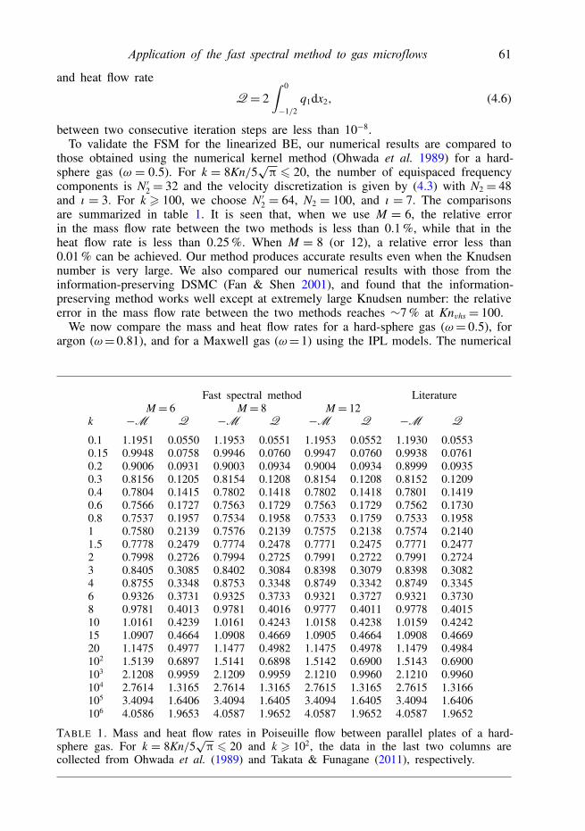
between two consecutive iteration steps are less than 10−8.To validate the FSM for the linearized BE, our numerical results are compared to

those obtained using the numerical kernel method (Ohwada et al. 1989) for a hard-sphere gas (ω = 0.5). For k = 8Kn/5

√π 6 20, the number of equispaced frequency

components is N ′2 = 32 and the velocity discretization is given by (4.3) with N2 = 48and ı = 3. For k > 100, we choose N ′2 = 64, N2 = 100, and ı = 7. The comparisonsare summarized in table 1. It is seen that, when we use M = 6, the relative errorin the mass flow rate between the two methods is less than 0.1 %, while that in theheat flow rate is less than 0.25 %. When M = 8 (or 12), a relative error less than0.01 % can be achieved. Our method produces accurate results even when the Knudsennumber is very large. We also compared our numerical results with those from theinformation-preserving DSMC (Fan & Shen 2001), and found that the information-preserving method works well except at extremely large Knudsen number: the relativeerror in the mass flow rate between the two methods reaches ∼7 % at Knvhs = 100.

We now compare the mass and heat flow rates for a hard-sphere gas (ω= 0.5), forargon (ω= 0.81), and for a Maxwell gas (ω= 1) using the IPL models. The numerical

Fast spectral method LiteratureM = 6 M = 8 M = 12

k −M Q −M Q −M Q −M Q

0.1 1.1951 0.0550 1.1953 0.0551 1.1953 0.0552 1.1930 0.05530.15 0.9948 0.0758 0.9946 0.0760 0.9947 0.0760 0.9938 0.07610.2 0.9006 0.0931 0.9003 0.0934 0.9004 0.0934 0.8999 0.09350.3 0.8156 0.1205 0.8154 0.1208 0.8154 0.1208 0.8152 0.12090.4 0.7804 0.1415 0.7802 0.1418 0.7802 0.1418 0.7801 0.14190.6 0.7566 0.1727 0.7563 0.1729 0.7563 0.1729 0.7562 0.17300.8 0.7537 0.1957 0.7534 0.1958 0.7533 0.1759 0.7533 0.19581 0.7580 0.2139 0.7576 0.2139 0.7575 0.2138 0.7574 0.21401.5 0.7778 0.2479 0.7774 0.2478 0.7771 0.2475 0.7771 0.24772 0.7998 0.2726 0.7994 0.2725 0.7991 0.2722 0.7991 0.27243 0.8405 0.3085 0.8402 0.3084 0.8398 0.3079 0.8398 0.30824 0.8755 0.3348 0.8753 0.3348 0.8749 0.3342 0.8749 0.33456 0.9326 0.3731 0.9325 0.3733 0.9321 0.3727 0.9321 0.37308 0.9781 0.4013 0.9781 0.4016 0.9777 0.4011 0.9778 0.401510 1.0161 0.4239 1.0161 0.4243 1.0158 0.4238 1.0159 0.424215 1.0907 0.4664 1.0908 0.4669 1.0905 0.4664 1.0908 0.466920 1.1475 0.4977 1.1477 0.4982 1.1475 0.4978 1.1479 0.4984102 1.5139 0.6897 1.5141 0.6898 1.5142 0.6900 1.5143 0.6900103 2.1208 0.9959 2.1209 0.9959 2.1210 0.9960 2.1210 0.9960104 2.7614 1.3165 2.7614 1.3165 2.7615 1.3165 2.7615 1.3166105 3.4094 1.6406 3.4094 1.6405 3.4094 1.6405 3.4094 1.6406106 4.0586 1.9653 4.0587 1.9652 4.0587 1.9652 4.0587 1.9652

TABLE 1. Mass and heat flow rates in Poiseuille flow between parallel plates of a hard-sphere gas. For k = 8Kn/5

√π 6 20 and k > 102, the data in the last two columns are

collected from Ohwada et al. (1989) and Takata & Funagane (2011), respectively.

62 L. Wu, J. M. Reese and Y. Zhang

Hard sphereArgonMaxwell 0.1

0.3

0.5

0.7

0.1

0.3

0.5

0.7

0.9

1.2

1.4

1.6

1.8

2.0

1.0

0.8

1.0

1.2

1.4

10–1 100 101 102

10–1 100 101 102 10–1 100 101 102

10–1 100 101 102

0.5

0.50.40.30.20.09

0.11

0.13

0.15

0.7

0.755

0.765

0.775

0.9

(a) (b)

(d)(c)

FIGURE 1. (Colour online) Comparisons of mass and heat flow rates for different IPLmolecular models in Poiseuille gas flow between parallel plates. (a) Mass flow rate −Mand (b) heat flow rate Q, at αa = 1.0; (c) −M and (d) Q, at αa = 0.8. Here αarepresents the wall accommodation coefficient, where the boundary condition at x2=−0.5is h(v1, v2, v3, x2 =−0.5)= (1− αa)h(v1,−v2, v3, x2 =−0.5) for v2 > 0.

results are shown in figure 1. We denote as Knc (≈ 0.9) the Knudsen number at whichthere is the Knudsen minimum in the mass flow rate. When Kn>Knc (or Kn<Knc),the mass flow rate decreases (or increases) as the viscosity index ω increases, fora fixed value of Kn. For instance, at Kn = 10, the mass flow rate of the Maxwellgas is ∼94 % that of the hard-sphere gas when αa = 1. The underlying mechanismfor this may be understood in terms of the effective collision frequency: for thesame value of shear viscosity, the average collision frequency

∫νeq(v)feqdv/

∫feqdv

increases with ω (see figures 12 and 13 in Wu et al. 2013 and the corresponding texttherein). Therefore, Maxwell molecules have a greater effective collision frequency(and a smaller effective Kn) than hard-sphere molecules. Since at large Kn the massflow rate increases with Kn, the Maxwell gas has a lower mass flow rate than thehard-sphere gas. Conversely, since at small Kn the mass flow rate decreases with Kn,when Kn < Knc, the Maxwell gas has a higher mass flow rate than the hard-spheregas, although the difference is very small. The heat flow rate behaves similarly tothe mass flow rate; that is, when Kn> 0.5 (or Kn< 0.5), the heat flow rate decreases(or increases) as ω increases, for a fixed value of Kn. The difference in flow rates

Application of the fast spectral method to gas microflows 63

10–2 10−1 100 101 10–2 10−1 100 101

0

2

4

6

8

10

12

He (IPL)He (LJ)Ne (IPL)Ne (LJ)Ar (IPL)Ar (LJ)Kr (IPL)Kr (LJ)Xe (IPL)Xe (LJ)

−4

0

4

8

12

(a) (b)

FIGURE 2. (Colour online) Relative differences in (a) the mass and (b) heat flow ratesbetween the molecular models and LJ potentials in Poiseuille gas flow between parallelplates for various δ. The subscripts SB indicate the results from Sharipov & Bertoldo(2009b).

between various gases with the same value of shear viscosity holds when the wallaccommodation coefficient αa is not 1, see figure 1(c,d).

Since IPL potentials are simplifications of the realistic LJ potential, it is interestingto check the accuracy of the collision kernels (2.3) and (2.7). Tables 2 and 3 comparethe mass flow rates and heat flow rates for five noble gases with the data of Sharipov& Bertoldo (2009b) for the LJ potential. For the IPL models, at a temperature of300 K, we use the viscosity index ωHe = ωNe = 0.66 (so only the results for heliumare shown), ωAr = 0.81 ' ωKr = 0.80 (so only the results for argon are shown), andωXe = 0.85. For the LJ potential, the potential depth ε of He, Ne, Ar, Kr, and Xeis 10.22kB, 35.7kB, 124kB, 190kB, and 229kB, respectively. The relative differencesbetween the mass and heat flow rates produced by the FSM and those in Sharipov &Bertoldo (2009b) are visualized in figure 2. For δ >0.2, the relative difference |MIPL−MSB|/|MSB| between the IPL models and LJ potentials is less than 1 %. For δ < 0.2,the relative difference increases as δ decreases. Specifically, at δ=0.01, the IPL modeloverestimates the mass flow rate by around 6.9 %, 10.5 %, 11.4 %, 11.7 %, and 11.0 %for He, Ne, Ar, Kr, and Xe, respectively. When the collision kernel (2.7) is used forthe LJ potential, at δ= 0.01, the LJ model overestimates the mass flow rate by around5.5 %, 6.0 %, 4.5 %, 3.3 %, and 2.6 % for He, Ne, Ar, Kr, and Xe, respectively. As δincreases, the relative difference quickly decreases. Similar behaviour can be observedfor the heat flow rate, except that the LJ models for Ar, Kr, and Xe underestimate theheat flow rate at small values of δ. Generally speaking, when compared to the solutionfor the realistic LJ potential, the LJ model yields closer results than the IPL model.

4.2. Thermal creep flow between parallel platesIn thermal creep flow, the wall temperature varies as T=T0(1+βTx1/`), where |βT |1. The VDF is expressed as f = feq + βT[x1feq(|v|2 − 5/2)+ h] and the linearized BEis given by (4.1) with the last term replaced by v1(|v|2 − 5/2)feq.

The Onsager–Casimir relation (Loyalka 1971; Sharipov 1994a,b; Takata 2009a,b)states that the mass flow rate in thermal creep flow is equal to the heat flow ratein Poiseuille flow:

∫V1[hT]dx2 =

∫q1[hP]dx2. Recently, Takata & Funagane (2011)

64 L. Wu, J. M. Reese and Y. Zhang

He

Ne

Ar

Kr

Xe

IPL

LJ

LJ

LJ

LJ

IPL

LJ

LJ

LJ

LJ

IPL

LJ

LJ

δFS

MFS

MSB

FSM

SBFS

MFS

MSB

FSM

SBFS

MFS

MSB

0.01

02.

852

2.81

42.

668

2.73

32.

581

2.78

82.

615

2.50

22.

577

2.49

52.

770

2.56

22.

497

0.02

02.

534

2.50

72.

424

2.44

42.

358

2.47

82.

349

2.28

02.

318

2.26

92.

463

2.30

62.

270

0.02

52.

438

2.41

42.

345

2.35

72.

287

2.38

52.

270

2.21

12.

242

2.19

92.

371

2.23

12.

199

0.04

02.

246

2.23

02.

182

2.18

52.

140

2.20

02.

115

2.07

22.

092

2.05

82.

188

2.08

22.

057

0.05

02.

160

2.14

82.

107

2.10

92.

073

2.11

72.

046

2.00

92.

025

1.99

52.

106

2.01

71.

993

0.10

01.

920

1.91

71.

893

1.89

41.

876

1.88

91.

853

1.83

01.

838

1.81

61.

881

1.83

21.

813

0.20

01.

726

1.72

81.

715

1.71

71.

707

1.70

41.

691

1.67

91.

681

1.66

81.

699

1.67

71.

665

0.25

01.

674

1.67

71.

667

1.66

81.

661

1.65

61.

647

1.63

71.

638

1.62

81.

651

1.63

51.

625

0.40

01.

584

1.58

71.

582

1.58

31.

580

1.57

21.

569

1.56

61.

564

1.55

91.

569

1.56

11.

557

0.50

01.

552

1.55

51.

552

1.55

11.

550

1.54

21.

541

1.54

01.

537

1.53

51.

540

1.53

61.

533

1.00

01.

504

1.50

51.

507

1.50

51.

508

1.50

21.

504

1.50

71.

504

1.50

71.

502

1.50

41.

507

1.60

01.

530

1.53

01.

534

1.53

11.

536

1.53

31.

536

1.54

01.

538

1.54

31.

534

1.53

91.

544

2.00

01.

565

1.56

51.

570

1.56

61.

572

1.57

01.

573

1.57

81.

576

1.58

21.

572

1.57

81.

583

2.50

01.

619

1.61

81.

624

1.62

01.

626

1.62

61.

629

1.63

41.

633

1.63

91.

628

1.63

51.

641

4.00

01.

813

1.81

11.

819

1.81

41.

822

1.82

41.

827

1.83

31.

833

1.83

91.

827

1.83

61.

842

5.00

01.

955

1.95

31.

963

1.95

71.

966

1.96

81.

971

1.97

81.

978

1.98

51.

972

1.98

11.

988

10.0

02.

723

2.72

12.

740

2.72

62.

743

2.74

42.

746

2.75

62.

755

2.76

42.

748

2.75

92.

768

TAB

LE

2.M

ass

flow

rate(−

2M)

inPo

iseu

ille

flow

ofva

riou

sga

ses

betw

een

para

llel

plat

esfo

rva

riou

sδ,

see

(2.6

).T

heda

tain

colu

mns

deno

ted

bySB

are

thos

ere

sults

from

Shar

ipov

&B

erto

ldo

(200

9b).

Application of the fast spectral method to gas microflows 65

He

Ne

Ar

Kr

Xe

IPL

LJ

LJ

LJ

LJ

IPL

LJ

LJ

LJ

LJ

IPL

LJ

LJ

δFS

MFS

MSB

FSM

SBFS

MFS

MSB

FSM

SBFS

MFS

MSB

0.01

01.

252

1.21

71.

142

1.14

31.

103

1.18

51.

043

1.05

51.

013

1.05

31.

166

1.00

11.

056

0.02

01.

092

1.06

61.

027

1.00

60.

990

1.03

30.

924

0.93

70.

899

0.93

31.

016

0.89

00.

935

0.02

51.

042

1.02

00.

989

0.96

50.

954

0.98

60.

890

0.90

00.

866

0.89

50.

970

0.85

70.

897

0.04

00.

942

0.92

70.

909

0.88

40.

878

0.89

30.

821

0.82

40.

801

0.81

80.

879

0.79

30.

819

0.05

00.

897

0.88

50.

870

0.84

70.

843

0.85

10.

790

0.79

00.

771

0.78

20.

838

0.76

40.

783

0.10

00.

764

0.76

10.

751

0.73

70.

734

0.72

90.

697

0.68

90.

682

0.68

00.

719

0.67

70.

679

0.20

00.

641

0.64

40.

637

0.63

10.

627

0.61

70.

604

0.59

50.

593

0.58

50.

610

0.58

90.

583

0.25

00.

604

0.60

70.

601

0.59

70.

593

0.58

30.

574

0.56

50.

564

0.55

60.

577

0.56

00.

554

0.40

00.

527

0.53

10.

526

0.52

50.

521

0.51

30.

509

0.50

30.

502

0.49

50.

509

0.49

90.

493

0.50

00.

492

0.49

50.

491

0.49

10.

487

0.48

00.

477

0.47

30.

473

0.46

70.

477

0.47

00.

465

1.00

00.

386

0.38

70.

385

0.38

60.

383

0.38

10.

381

0.37

90.

379

0.37

70.

380

0.37

90.

376

1.60

00.

316

0.31

60.

315

0.31

60.

314

0.31

50.

316

0.31

50.

316

0.31

50.

315

0.31

60.

315

2.00

00.

283

0.28

40.

282

0.28

40.

282

0.28

40.

285

0.28

40.

286

0.28

50.

284

0.28

60.

286

2.50

00.

252

0.25

20.

251

0.25

20.

251

0.25

40.

255

0.25

40.

256

0.25

60.

254

0.25

70.

256

4.00

00.

189

0.18

90.

188

0.19

00.

189

0.19

20.

193

0.19

30.

195

0.19

60.

193

0.19

60.

197

5.00

00.

162

0.16

20.

161

0.16

30.

162

0.16

60.

166

0.16

60.

168

0.16

90.

167

0.16

90.

170

10.0

00.

094

0.09

30.

093

0.09

40.

093

0.09

70.

097

0.09

70.

099

0.09

90.

098

0.10

00.

100

TAB

LE

3.H

eat

flow

rate(2

Q)

inPo

iseu

ille

flow

ofva

riou

sga

ses

betw

een

para

llel

plat

esfo

rva

riou

sδ.

The

data

inco

lum

nsde

note

dby

SBar

eth

ose

resu

ltsfr

omSh

arip

ov&

Ber

told

o(2

009b

).

66 L. Wu, J. M. Reese and Y. Zhang

−4 −3 −2 −1 0 1 2 3 4

−4 −3 −2 −1 0 1 2 3 4

−4 −3 −2 −1 0 1 2 3 40

0.02

0.04

0.06

0.08

0.10

0

0.02

0.04

0.06

0.08

0.10

0

0.02

0.04

0.06

0.08

0.10

(a) (b)

(c)

FIGURE 3. (Colour online) Demonstration of a strong Onsager–Casimir relation at themicroscopic level. Lines (or dots): velocity distribution functions (|v|2 − 5/2)hP inPoiseuille flow (or hT in thermal creep flow) at v1, v3 = 6/31 and Kn = 104. Thecurves correspond to, from top to bottom the hard-sphere, helium (IPL), argon (IPL), andMaxwell gases, respectively. (a) x2 =−0.5, (b) x2 =−0.25, (c) x2 = 0.

observed a strong relation, that is, at large Kn, V1[hT] and q1[hP] have identical spatialprofiles, i.e. V1[hT] = q1[hP] + O[Kn−1(ln Kn)2]. The VDFs obtained by our FSM infigure 3 show that a stronger Onsager–Casimir relation exists at the microscopic level,that is, hT ≈ (|v|2 − 5/2)hP, at large Kn, for various IPL models.

Because of the Onsager–Casimir relation, we compare only the heat flow rates inthermal creep flow for different potential models. The results are in table 4. For aparticular molecular model, the heat flow rate increase monotonically as δ decreases.As in the Poiseuille flow case, different molecular models have different flow rates atthe same value of shear viscosity; for IPL models, the heat flow rate always decreasesas ω increases.

The relative difference in heat flow rates is visualized in figure 4. At δ= 0.01, forHe, Ne, Ar, Kr, and Xe, the IPL models overestimate the heat flow rate relative toSharipov & Bertoldo (2009b) by 6.6 %, 10.3 %, 11.4 %, 11.7 %, and 11 %, while theLJ model overestimates the heat flow rate by 5.1 %, 5.7 %, 4.6 %, 3.5 %, and 2.9 %,respectively. As δ increases, the relative difference quickly decreases. This comparison,together with those for Poiseuille flows, indicate that, in the free-molecular regime,it is necessary to consider the LJ potential to get highly reliable results (Sharipov

Application of the fast spectral method to gas microflows 67

He

Ne

Ar

Kr

Xe

IPL

LJ

LJ

LJ

LJ

IPL

LJ

LJ

LJ

LJ

IPL

LJ

LJ

δFS

MFS

MSB

FSM

SBFS

MFS

MSB

FSM

SBFS

MFS

MSB

0.01

06.

269

6.18

25.

879

6.01

05.

684

6.14

05.

768

5.51

25.

691

5.49

66.

104

5.66

25.

500

0.02

05.

496

5.43

55.

263

5.30

15.

121

5.38

55.

109

4.95

85.

048

4.93

45.

354

5.02

44.

935

0.02

55.

255

5.20

25.

059

5.08

24.

936

5.15

14.

906

4.77

94.

850

4.75

45.

121

4.82

84.

754

0.04

04.

761

4.72

54.

626

4.63

24.

542

4.67

04.

491

4.40

44.

445

4.37

64.

644

4.42

74.

373

0.05

04.

532

4.50

54.

421

4.42

44.

353

4.44

84.

298

4.22

54.

257

4.19

74.

424

4.24

04.

193

0.10

03.

848

3.84

03.

792

3.79

33.

761

3.78

43.

709

3.66

93.

679

3.64

13.

766

3.66

63.

635

0.20

03.

196

3.20

03.

174

3.17

53.

162

3.15

13.

120

3.10

33.

098

3.08

03.

138

3.08

93.

074

0.25

02.

992

2.99

72.

977

2.97

72.

968

2.95

12.

929

2.91

82.

909

2.89

72.

940

2.90

12.

891

0.40

02.

569

2.57

52.

562

2.56

22.

560

2.53

82.

526

2.52

52.

511

2.50

82.

529

2.50

42.

502

0.50

02.

371

2.37

72.

367

2.36

72.

366

2.34

32.

335

2.33

72.

321

2.32

22.

336

2.31

62.

317

1.00

01.

772

1.77

61.

770

1.77

01.

771

1.75

21.

750

1.75

61.

741

1.74

51.

748

1.73

71.

741

1.60

01.

387

1.39

11.

385

1.38

71.

387

1.37

31.

371

1.37

71.

365

1.36

91.

369

1.36

21.

366

2.00

01.

216

1.21

91.

213

1.21

51.

216

1.20

31.

202

1.20

71.

197

1.20

11.

200

1.19

41.

198

2.50

01.

054

1.05

71.

051

1.05

41.

053

1.04

31.

042

1.04

61.

038

1.04

11.

040

1.03

61.

039

4.00

00.

752

0.75

40.

750

0.75

20.

752

0.74

50.

745

0.74

70.

742

0.74

40.

743

0.74

00.

743

5.00

00.

631

0.63

30.

629

0.63

10.

630

0.62

50.

625

0.62

70.

622

0.62

50.

623

0.62

10.

624

10.0

00.

347

0.34

80.

345

0.34

70.

346

0.34

40.

344

0.34

50.

343

0.34

40.

343

0.34

20.

344

TAB

LE

4.H

eat

flow

rate(2

Q)

inth

erm

alcr

eep

flow

ofva

riou

sga

ses

betw

een

para

llel

plat

esfo

rva

riou

sδ.

The

data

inco

lum

nsde

note

dby

SBar

eth

ose

resu

ltsfr

omSh

arip

ov&

Ber

told

o(2

009b

).

68 L. Wu, J. M. Reese and Y. Zhang

10–2 10−1 100 101

0

2

4

6

8

10

12

He (IPL)

He (LJ)Ne (IPL)

Ne (LJ)

Ar (IPL)

Ar (LJ)

Kr (IPL)

Kr (LJ)

Xe (IPL)

Xe (LJ)

FIGURE 4. (Colour online) Relative difference in the heat flow rate between differentmolecular models and the LJ potential in thermal creep flow between parallel plates as afunction of δ.

& Strapasson 2012; Venkattraman & Alexeenko 2012; Sharipov & Strapasson 2013).However, the LJ model with the collision kernel (2.7) can produce mass and heat flowrates with a relative error less than 2 % when δ > 0.04 or, equivalently, Kn< 22.

In the free-molecular limit, it has previously been found that the mass flow ratesin Poiseuille and thermal creep flows increase logarithmically with the Knudsennumber (Cercignani & Daneri 1963; Takata & Funagane 2011). Our numericalresults show that the heat flow rate in thermal creep flow can also be fitted to alogarithmic function of Kn, namely Q[hT] = −0.6345 ln(Kn) − Q0 in the region105 <Kn< 2× 106, where the constant Q0 is 0.2679, 0.1762, 0.07371, and −0.09903for hard-sphere, helium, argon, and the Maxwell gases when the IPL model is used,respectively.

4.3. Poiseuille and thermal creep flow along a rectangular tubeWe now consider rarefied gases in a long straight tube that lies along the x3 axis.The cross-section is uniform and rectangular, so that −A`/2< x1 <A`/2 and −`/2<x2 < `/2, where A is the aspect ratio. The linearized BE in dimensionless form forPoiseuille flow along this rectangular tube is

v1∂h∂x1+ v2

∂h∂x2=Lg(h)− νeq(v)h− v3feq, (4.7)

while v3 should be replaced by v3(|v|2 − 5/2

)for a thermal creep flow. Due

to symmetry, only one quarter of the spatial domain is considered. The massflow rate is defined as M = (4/A) ∫ 0

−1/2

∫ 0−A/2 V3dx1dx2 and the heat flow rate is

Q= (4/A) ∫ 0−1/2

∫ 0−A/2 q3dx1dx2, where V3 =

∫v3hdv and q3 =

∫ (|v|2 − 5/2)v3hdv.

Application of the fast spectral method to gas microflows 69

This problem was first solved for a hard-sphere gas by the numerical kernelmethod (Doi 2010) and then by the low-noise DSMC method (Radtke et al. 2011).To compare the numerical accuracy and efficiency of our new FSM, we first considerthe thermal creep flow at Knvhs= 0.1 and A= 2. We use a 50× 50 non-uniform spatialgrid (see (4.2)), 32× 32 non-uniform velocity grids ((4.3) with ı = 3) in the v1 andv2 directions, and 12 uniform mesh points in the v3 direction. The FSM with M = 6yields M = 0.0478, compared to 0.048 by Doi (2010) and 0.0473 by Radtke et al.(2011). We then consider Poiseuille flow in the square tube; with a 25 × 25 spatialcell mesh, 32 × 32 × 24 frequency components, and M = 6, we obtain M = 0.3808and 0.3966, Q = 0.1365 and 0.1874 for Knvhs = 1 and 10, respectively, compared toDoi’s 0.381 and 0.396 for M , and 0.136 and 0.187 for Q. The computational timeis 100 and 40 s, respectively (our Fortran program runs on a computer with an IntelXeon 3.3 GHz CPU, and only one core is used), compared to the low-noise DSMCthat takes 66 and 12 min , respectively. (This DSMC code runs on a single core ofan Intel Q9650, 3.0 GHz Core 2 Quad processor. The time is obtained when thereis better than 0.1 % statistical uncertainty in the mass flow rate. To achieve the samelevel of uncertainty in the velocity field, the low-noise DSMC would need 240 and120 min, respectively). These comparisons indicate that the FSM is both accurate andefficient new numerical method.

We observe that the difference in mass and heat flow rates between differentmolecular models is very small when A = 1. Although the difference increases withA, at A = 10, |(MAr −MHe)/MAr| is only 1.6 % at δ = 0.01, while that at A =∞is 7.6 %, when the LJ model is used. So, in the following numerical simulation weonly use the IPL model.

We now compare our numerical results with recent experiments on the reduced massflow rate in Poiseuille flow (Ewart et al. 2007). The tube cross-section is rectangular,with an aspect ratio of A = 52.45. The working gas is helium and we take the IPLmodel with ω= 0.66. In the spatial discretization, 100 and 50 non-uniform grid pointsare used in the x1 and x2 directions, respectively. The number of velocity grids is 32×32×12, the frequency components are 32×32×24, and the number of discrete anglesis M = 6. Different wall accommodation coefficients αa are used: the wall boundarycondition is given by h(v1, v2, v3, x1=−A/2, x2)= (1−αa)h(−v1, v2, v3, x1=−A/2, x2)for v1 > 0 and h(v1, v2, v3, x1, x2 =−1/2)= (1− αa)h(v1,−v2, v3, x1, x2 =−1/2) forv2 > 0. The obtained mass flow rate M is transformed to the reduced mass flow rateG via the following equation (Sharipov & Seleznev 1994):

G(δin, δout)= 2δout − δin

∫ δout

δin

M (δ)dδ, (4.8)

where the subscripts ‘in’ and ‘out’ stand for the inlet and outlet, respectively. Thereduced mass flow rate G no longer depends on the local pressure gradient, but onlyon the mean value of pressure; so the parameter δm at the mean pressure of the tubeis also introduced. We consider the published experimental data where the inlet tooutlet pressure ratio is 5, so that δin = 5δm/3 and δout = δm/3. The mass flow rate Mis obtained at discrete values of the rarefaction parameter. The reduced mass flow rateis calculated by (4.8), where M at an unknown δ is obtained by cubic interpolation.Comparisons between the numerical and experimental data are visualized in figure 5.When δ> 6, the experimental data agree well with the numerical results from the BEif αa = 0.92. In the region 1 6 δ < 6, the experimental data agree with the numericalresults if αa = 0.92 ∼ 1. For 0.2 6 δ 6 1, the mass flow rates from the BE withαa = 0.92 agree with the experimental measurements. When δ 6 0.1, the BE withαa = 0.95∼ 1 agrees well with the experimental results.

70 L. Wu, J. M. Reese and Y. Zhang

10−2 10−1 100 101

1.5

1.7

1.9

2.1

2.3

2.5

2.7

2.9

G

Experiment

= 1.00= 0.95

= 0.92

FIGURE 5. (Colour online) Comparison of the FSM-calculated reduced mass flow rate Gin Poiseuille flow along a rectangular tube (aspect ratio 52.45) with the experimental dataof Ewart et al. (2007), for various values of the wall accommodation coefficient αa.

Note that the advantage of the FSM over the DSMC method becomes moreprofound for a series of simulations with the same spatial geometry but differentvalues of Kn. Sorting Kn in descending order, the converged VDF at the previousKn can be used as the initial condition for the FSM for those subsequent Kn. Inthis way, the computational efficiency can be improved further. For example, for thisPoiseuille flow problem, it takes 4.4 h to compute the solution for Kn = 0.1 whenthe initial VDF is the global equilibrium one, but only 2 h when the initial VDF istaken as the solution at Kn= 0.15.

5. Numerical results for the nonlinear Boltzmann equationIn this section, a number of two-dimensional simulations using the nonlinear BE

are carried out in the transition flow regime (0.1 6 Kn 6 10) and the free-molecularregime using the IPL models. The influence of the IPL models on the macroscopicflow properties is assessed, and the applicability of the linear BCO for microflowswith large temperature variations is evaluated. A linear scaling law is proposed forthe flow velocities in thermally driven flows in the free-molecular regime. Specifically,thermal creep flow inside a closed channel is analysed, where the flow pattern can bewell explained as the superposition of both the velocity profiles of linearized Poiseuilleand thermal creep flow between parallel plates.

5.1. Lid-driven cavity flowConsider the lid-driven flow in a square cavity, as has been previously studied usingDSMC (John, Gu & Emerson 2010, 2011). Since the gas velocity near the lower

Application of the fast spectral method to gas microflows 71

wall is small, the DSMC solution is extremely time-consuming. Even when thevelocity of the moving upper lid is so small that the linearized BE can be applied,the low-noise DSMC method (Radtke et al. 2011) takes more than 1 day to achievereasonably resolved results at Knvhs = 0.1.

We solve this problem (for argon gas, an upper lid velocity of 50 m s−1, and awall temperature of 273 K) in a 51 × 51 non-uniform spatial grid, see (4.2). Theminimum length of the spatial cell is 7.8× 10−5, while the maximum is 0.0375, withmost of the grid points located near the walls. For Knvhs = 0.1 and 1, 32× 32× 12grid points in velocity space are used, while for Knvhs = 10, there are 64× 64× 12velocity grid points, with most of the grid points located in v1, v2 ∼ 0 to capture thediscontinuities in the VDF. The number of frequency components is 32 × 32 × 24.The BCO is approximated by the FSM with M = 6, and the spatial derivatives areapproximated by second-order upwind finite differences. We solve the discretized BEby the implicit scheme in an iterative manner. At the (k + 1)th iteration step, theVDF at the wall (entering the cavity) is determined according to the diffuse boundarycondition, using the VDF at the same position (but leaving the cavity) at the previousiteration step. This numerical scheme is much faster than an explicit time-dependenttechnique because no Courant–Friedrichs-Lewy condition is imposed (Frangi, Ghisi &Frezzotti 2007). However, the disadvantage is that, when the mass flux entering thecavity at the (k+ 1)th step (which is equal to that leaving the cavity at the kth step)is not equal to that leaving the cavity at the (k + 1)th step, the total mass insidethe cavity is not conserved. To overcome this, at the end of each iteration step, asimple correction of the VDF by a factor equal to the initial total mass divided by thecurrent total mass is introduced. This is sufficient to recover the correct steady-stateconditions, and was introduced by Mieussens & Struchtrup (2004).

The convergence rate of our iterative scheme is proportional to the Knudsen number.For Knvhs = 0.1 and 1, starting from the global equilibrium state, the FSM takes 110and 14 min, respectively, to produce a converged solution, which is when the errorbetween two consecutive iteration steps,

‖ε‖2 =max

√√√√√√√∫|Vk+1

1 − Vk1 |2dx1dx2∫

|Vk1 |2dx1dx2

,

√√√√√√√∫|Vk+1

2 − Vk2 |2dx1dx2∫

|Vk2 |2dx1dx2

, (5.1)

is less than 10−5.Figure 6 shows the calculated temperature contours and streamlines in the lid-driven

cavity flow of argon gas with diffuse boundary conditions. Compared to DSMC, thesesolutions are free of noise. We have also simulated the flow of a hard-sphere gas, withthe same values of the normalized wall velocity (i.e. 0.148) and shear viscosity (theKnudsen numbers Kn are the same, but the Knvhs are different). Comparisons of thevelocity, temperature, and heat flux profiles between the two IPL molecular models areshown in figure 7, and demonstrate that the molecular model has little influence onthe flow pattern. This may explain why, for the same problem, the Bhatnagar–Gross–Krook (BGK) and Shakhov kinetic models can both produce excellent results that arein agreement with DSMC data (Huang, Xu & Yu 2012).

72 L. Wu, J. M. Reese and Y. Zhang

0 0.1 0.3 0.5 0.7 0.9

0.2

0.4

0.6

0.8

1.0

270.5

272.5

274.5

276.5

0 0.1 0.3 0.5 0.7 0.9

0.2

0.4

0.6

0.8

1.0

270.5

272.5

274.5

276.5

0 0.1 0.3 0.5 0.7 0.9

0.2

0.4

0.6

0.8

1.0

270.0

272.0

274.0

276.0

0 0.1 0.3 0.5 0.7 0.9

0.2

0.4

0.6

0.8

1.0

270.0

272.0

274.0

276.0

0 0.1 0.3 0.5 0.7 0.9

0.2

0.4

0.6

0.8

1.0

x1 x1

x2

x2

x2

269.0

271.5

273.5

275.5

0 0.1 0.3 0.5 0.7 0.9

0.2

0.4

0.6

0.8

1.0

269.0

272.0

274.0

276.0

(a)

(c) (d)

( f )(e)

(b)

FIGURE 6. Temperature contours and streamlines (velocity: left-hand column; heat flux:right-hand column) in the lid-driven cavity flow of argon gas. The Knudsen number Knvhsis: (a,b) 0.1, (c,d) 1, and (e,f ) 10. The lid moves from left to right, and the temperatureis not normalised.

5.2. Thermally driven flows5.2.1. Thermal creep flow inside a closed channel

Consider thermal creep flow in a two-dimensional closed rectangular channel witha length-to-width ratio of 5. The temperature at the right-hand side is set to be twicethat of the left-hand side, while the temperature of the top and bottom walls varieslinearly along the channel. Using the mean density, the temperature of the left-handwall, and the channel width, Kn is set to be 0.08, 0.2, 0.25, 0.6, 2, and 10 in thecases we investigate. Figure 8 presents the resulting streamlines and the temperaturedistributions inside the channel for the flow of argon gas. Due to symmetry, only the

Application of the fast spectral method to gas microflows 73

0 0.2 0.4 0.6 0.8 1.0x1, x2

271

272

273

274

275

Tem

pera

ture

(e)

(c) (d)

V1 / Vwall

−0.2 0 0.2 0.4 0.6

0 0.2 0.4 0.6 0.8 1.0x1

−6 −2 2 6 10 14

0

0.2

0.4

0.6

0.8

1.0

0

0.2

0.4

0.6

0.8

1.0

x2

x2

(b)

0 0.2 0.4 0.6 0.8 1.0x1

−0.20

−0.15

−0.10

−0.05

0

0.05

0.10

0.15V

2 / V

wal

l

(a)

−3

−2

−1

0

1

2

q 2 ×

103

q1 × 103

FIGURE 7. Comparisons of the velocity, heat flux, and temperature profiles between argonand hard-sphere gases in lid-driven cavity flow. The solid (or dashed) lines are the resultsfor argon with Knvhs= 0.1 (or 10). The circles (or stars) are the results for the hard-spheregas with Knvhs = 0.132 (or 13.2). (a,c) at x2 = 0.5. (b,d) at x1 = 0.5. (e) Filled (open)markers: x1 = 0.5 (x2 = 0.5).

lower half of the spatial domain is shown. Unlike thermal creep in an open channel,where the flow straightforwardly moves towards the hot region, the thermal creep flowin a closed channel exhibits richer phenomena. At Kn = 0.08, the gas flows fromthe cold region to the hot region along the bottom wall, and returns in the centralregion. At Kn = 0.2, the flow still moves from hot to cold in the central region;however, near the lower wall the flow moves towards the hot region when x1 < 2and towards the cold region for x1 > 2, i.e. a circulation emerges near the lowerhot corner of the domain. At Kn = 0.25, the circulation near the lower wall grows,which divides the flow in the central region into two circulation zones. The lowercirculation zone keeps expanding, and pushes the other two circulations in the centralregion towards the left- and right-hand boundaries, as Kn increases. At Kn = 0.6,the flow direction is reversed (as compared to that when Kn = 0.08) and only onecirculation zone remains near the left-hand wall. The reversal of the flow direction

74 L. Wu, J. M. Reese and Y. Zhang

x2

x2

x2

x2

x2

x2

0 0.5 1.0 1.5 2.0 2.5 3.0 3.5 4.0 4.5 5.0

0.2

0.4

0 0.5 1.0 1.5 2.0 2.5 3.0 3.5 4.0 4.5 5.0

0.2

0.4(b)

(a)

0 0.5 1.0 1.5 2.0 2.5 3.0 3.5 4.0 4.5 5.0

0.2

0.4(c)

0 0.5 1.0 1.5 2.0 2.5 3.0 3.5 4.0 4.5 5.0

0.2

0.4(d)

0 0.5 1.0 1.5 2.0 2.5 3.0 3.5 4.0 4.5 5.0

0.2

0.4(e)

x1

0 0.5 1.0 1.5 2.0 2.5 3.0 3.5 4.0 4.5 5.0

0.2

0.4( f )

FIGURE 8. (Colour online) Temperature contours and velocity streamlines in the thermalcreep flow of argon gas within a closed rectangular channel (only the lower half-domain isshown). In each figure, from left to right, the non-dimensional temperature of each contouris 1+ 0.1i, where i= 1, 2, . . . , 9. (a) Kn= 0.08, (b) Kn= 0.2, (c) Kn= 0.25, (d) Kn= 0.6,(e) Kn= 2, (f ) Kn= 10.

Application of the fast spectral method to gas microflows 75

50 60 80100 150 200 300 500 800 1000

10–5

10−4

10−3

Hard sphereArgonMaxwell

(a) (b)

−12 −8 −6 −2 2 6

x2

Hard sphere Kn = 1000Hard sphere Kn = 100Argon Kn = 1000Argon Kn = 100Maxwell Kn = 1000Maxwell Kn = 100

0

0.1

0.2

0.3

0.4

0.5

FIGURE 9. (Colour online) (a) The horizontal velocity varying with Kn in thermalcreep flow inside a closed rectangular channel, in the free-molecular regime. In thisdouble-logarithmic diagram, the three lines have a slope of 1, demonstrating that thevelocity magnitude is proportional to 1/Kn. (b) Examples of the linear scalability in thefree-molecular regime of the horizontal velocity at x1 = 1.4825.

persists but the circulations near the left-hand wall gradually disappear as the Knudsennumber increases further, for instance, to Kn= 2. By Kn= 10, the gas near the bottomwall moves from hot to cold, and two clockwise circulations emerge near the left-and right-hand sides. Finally, when the flow enters the free-molecular regime, thestreamline pattern does not change, but the velocity magnitudes are proportional to1/Kn, see figure 9. The magnitudes of density, pressure, and temperature, however,remain unchanged irrespective of the Knudsen number in this regime.

Comparison of the velocity profiles for different molecular models at the start andthe end of the transition flow regime are shown in figure 10; it can be seen that themolecular model affects the velocity magnitudes significantly.

The flow patterns shown in figure 8 can be understood qualitatively as follows.Starting from the global equilibrium state, the temperature gradient drives the gasmolecules to move from cold to hot (thermal creep flow). This process increases thepressure at the right-hand side of the channel while decreasing the pressure at the left.Then, the pressure gradient causes the gas molecules to move to the left (Poiseuilleflow). The steady state is reached when the effects of Poiseuille and thermal creepflows cancel each other out, that is, when the net mass flow rate across the linesperpendicular to the top and bottom walls is zero. The horizontal velocity profile canbe analysed by assuming the wall temperature gradient to be small (i.e. the channelis long enough) so that the BE can be linearized. In this case, we can directly use thevelocity profiles obtained in § 4. Figure 11 plots the net velocity profiles in the linearsuperposition of Poiseuille and thermal creep flows between parallel plates where thenet mass flow rate is zero. The flow velocities are normalized; in real problems, thehorizontal velocity is given by (see the first paragraph in § 4.2):

V1 = βT

V1[hT] −M [hT]

M [hP]V1[hP], (5.2)

where βT is the temperature gradient; in this case, it is about 1/5.Now the horizontal velocity profiles in figure 11 can be used to explain the

flow patterns in figure 8. From figure 11 we find that, when Kn = √π/20, the

76 L. Wu, J. M. Reese and Y. Zhang

0 1.0 2.0 3.0 4.0 5.0x1

x1

x2

Hard sphereArgonMaxwell

−18

−14

−10

−6

−2

(a) (b)

(c) (d)

−15 −10 −5 0 5 10 150

0.1

0.2

0.3

0.4

0.5

x2

0

0.1

0.2

0.3

0.4

0.5

0 1 2 3 4 50

1

2

3

4

−10 −8 −6 −4 −2 0 2 4

FIGURE 10. Velocity profiles for thermal creep flow within a closed rectangular channel;(a,b) Kn = 0.08, and (c,d) Kn = 10 are represented by the red and blue lines andaxis labels, respectively. (a,c) Horizontal velocity along the central horizontal line. (b,d)Horizontal velocity along the central vertical line.

net horizontal velocity is positive when x2 < 0.25 and negative otherwise, whichagrees well with the flow pattern in figure 8(a). Also, from figure 10(a) we findthat, at Kn = 0.08, V1(x2 = 0.5) ' −0.0018 near the left-hand side of the channel,which is well predicted by (5.2) when we choose Kn = √π/20 and x2 = 0.5:V1(x2 = 0.5) ' (−0.009)/5 = −0.0018. Furthermore, as Kn increases, the magnitudeof the horizontal velocity at x2= 0.5 decreases (figure 11). This is in accordance withthe horizontal velocity profiles shown in figure 10(a), where the velocity magnitudedecreases as x1 increases from 1 to 4, because the local Knudsen number increasesalong the channel as a result of increasing temperature and decreasing particle numberdensity. When Kn = √π/10 (and

√π/8), the net horizontal velocity in figure 11 is

positive when 0.26 > x2 > 0.009 (and 0.28 > x2 > 0.023) and negative otherwise.This explains the flow patterns at the right-hand side of the channel, as shown infigure 8(b). As Kn increases, the extent of the region near the bottom wall wherethe velocity is negative increases (figure 11), so that the circulation near the bottomwall in figure 8(c) is larger than that in figure 8(b). When Kn increases above acritical value of around

√π/5, the horizontal velocity in figure 11 is negative when

x2 is smaller than some fixed value x2c and positive otherwise. In this case, the flowdirection is completely reversed in comparison with that at small Knudsen numbers.When Kn>

√π/2, the fixed value is x2c = 0.2. In figure 8(d–f ), we see that the gas

moves from left to right if x2 < 0.2, and moves right to left if x2 > 0.2.

Application of the fast spectral method to gas microflows 77

−0.020 −0.015 −0.010 −0.005 0 0.005 0.0100

0.05

0.10

0.15

0.20

0.25

0.30

0.35

0.40

0.45

0.50

x2

FIGURE 11. (Colour online) Net horizontal velocity profiles obtained by linearsuperposition of the velocity profiles of Poiseuille and thermal creep flows betweenparallel plates, which result in zero mass flow rate. The walls are at x2 = 0 and x2 = 1and the working gas is argon, where the IPL model with ω= 0.81 is used.

Note that the above analysis is valid at positions far from the left- and right-handwalls; near the ends of the channel, the horizontal velocity is nearly zero and theabove analysis fails. This end effect becomes dominant in the whole channel whenthe molecular mean free path is of the order of half the distance between the left- andright-hand walls. When the mean free path is much larger than the wall distance, fromfigures 8 and 9 we find that the streamline pattern does not change very much, but thevelocity magnitude is inversely proportional to the Knudsen number. In other words,at large Knudsen numbers, the flow pattern is determined by the velocity profiles infigure 11 at a critical Knudsen number. In our numerical simulations, we find thatthe critical Knudsen number varies linearly with the length-to-height ratio A of thechannel:

Knc ' 0.35A. (5.3)

For instance, when A= 0.25, the end effect becomes dominant when Knc > 0.09, andthe flow pattern at KnKnc is similar to the flow pattern at Knc. Figure 11 shows thatat Kn= 0.09 the molecules move from left to right near the bottom wall, and returnto the left at x2 = 0.5, which is exactly the case shown in figure 12(a). For A= 0.5,Knc = 0.18 ' √π/10, and from figure 11 we see the horizontal flow velocity turnsfrom negative to positive and then back to negative as we move from the bottom wallto the central region, which is the same as in figure 12(b). The aspect ratio A= 1 is acritical case, since near Knc = 0.35'√π/5, the horizontal velocity at x2 = 0.5 could

78 L. Wu, J. M. Reese and Y. Zhang

(b)

0 0.1 0.2 0.3 0.4 0.5

(c)

0 0.2 0.4 0.6 0.8 1.0

0.1

0.2

0.3

0.4

0.5

x2

x2

(a)

0 0.125 0.250

0.1

0.2

0.3

0.4

0.5

0.1

0.2

0.3

0.4

0.5

x1

x1 x1 x1

(d)

0 0.2 0.4 0.6 0.8 1.0 1.2 1.4 1.6 1.8 2.0

0.1

0.2

0.3

0.4

0.5

FIGURE 12. Thermal creep flow patterns of argon gas (IPL model with ω = 0.81) inthe free-molecular regime at different values of length-to-height ratio A: (a) A= 0.25, (b)A= 0.5, (c) A= 1, and (d) A= 2.

be negative or positive, depending on whether the local Knudsen number is smalleror larger than

√π/5. That is why the flow pattern shown in figure 12(c) is more

complicated. For A=2, where Knc=0.7, the flow pattern is simpler, and the moleculesmove from the hot to the cold region near the bottom and return from the cold tothe hot region near x2 = 0.5, see figure 12(d). For Kn< Knc, the horizontal velocityprofiles can be analysed using the data in figure 11.

5.2.2. Flow induced by a spatially periodic wall temperatureConsider the gas flow between two parallel plates that have a spatially periodic

temperature: the upper (x2= `) and lower plates (x2= 0) have the temperature T0(1−0.5 cos 2πx1). Due to symmetry, the spatial domain is chosen as 06 x1, x2 6 1/2. Thespecular reflection boundary condition is chosen for the left-hand, upper, and right-hand boundaries, while the diffuse boundary condition is employed at the lower wall.Using the mean density, mean temperature T0, and the wall distance `, the unconfinedKnudsen number Kn is chosen to be 0.1, 1, and 10. In the spatial discretization, 51equispaced points are used in the x1 direction and 51 non-uniform points (see (4.2))are placed in the x2 direction, with most of the points close to the lower wall. In thediscretization of the velocity space, 64×64×16 (maximum velocity L=7.5, L2=5 in(4.3) with ı = 3) grid points are used when Kn= 0.1 and 1, while 128× 128× 16 gridpoints are used when Kn= 10. The number of frequency components is 32× 32× 32.Even with such a large number of velocity grid points, the FSM with M = 6 takesonly ∼150 min to converge to ‖ε‖2 less than 10−5 at Kn= 0.1.

The temperature contours and velocity streamlines are shown in figure 13. The gasmoves from the cold to the hot region near the lower wall, while it returns from hotto cold around the central horizontal region. The circulation centre approaches thelower wall as Kn increases. The marginal VDFs, which become more complicatedas Kn increases, are shown in figure 14, and large discontinuities at the lower wall

Application of the fast spectral method to gas microflows 79

0 0.1

0.05

0.15

0.25

0.35

0.45

0.05

0.15

0.25

0.35

0.45

0.05

0.15

0.25

0.35

0.45

0.2 0.3 0.4 0.5

0 0.1 0.2 0.3 0.4 0.5

0.7

0.8

0.9

1.0

1.1

0.7

0.8

0.9

1.0

1.1

1.2

0 0.1 0.2 0.3 0.4 0.5

0.7

0.9

1.1

1.3

x1

x1

x2

x2

x1

(a) (b)

(c)

FIGURE 13. Contour plots of the temperature, and the velocity streamlines in argon gassubjected to a spatially periodic wall temperature: (a) Kn= 0.1, (b) Kn= 1, (c) Kn= 10.

(a) (b)

0.010.020.030.040.050.060.070.080.090.100.11

0.02

0.04

0.06

0.08

0.10

0.12

0.14

0.16

FIGURE 14. Contour plots of the marginal VDF,∫

f dv3, for hard sphere gas for (a)Kn = 1 and (b) Kn = 10. In each figure, from bottom to top, x2 = 0.5, 0.25, and 0.5,respectively; from left to right, x1 = 0, 0.25, and 0.5, respectively. The velocity regionshown is [−2, 2] × [−2, 2].

and fine structures are clearly seen. This demonstrates the necessity of using a largenumber of velocity grid points in the v1 and v2 directions at large Kn, in order to get

80 L. Wu, J. M. Reese and Y. Zhang

0 0.05 0.15 0.25 0.35 0.45

0.5

1.0

1.5

2.0

2.5

3.0

3.5

4.0

4.5

Hard sphere: nonlinearHard sphere: linearArgon: nonlinearArgon: linearMaxwell: nonlinearMaxwell: linear

x1

x2

V2

V1

(a) (b)

0 0.2 0.4 0.6 0.8 1.0 1.2 1.4 1.6

0.05

0.10

0.15

0.20

0.25

0.30

0.35

0.40

0.45

0.50

FIGURE 15. (Colour online) Comparisons of the velocity profiles predicted by the fullnonlinear and the linearized BEs, and for different molecular models. The unconfinedKnudsen number is Kn = 1 and the temperature of the top and bottom walls varies asT0(1− 0.5 cos 2πx1). (a) x2 = 0, (b) x1 = 0.5.

a high resolution. The flow velocities for different molecular models are comparedin figure 15: the maximum velocity increases with the viscosity index. We havealso investigated the flow in the free-molecular regime and find that the velocitymagnitudes are inversely proportional to the Knudsen number, as was the case forthermal creep flow inside closed channels.

Note that this problem has also been solved by the low-noise DSMC method, basedon the linearized BE (Radtke et al. 2011): from figure 14 we see that the VDFsdeviate significantly from the equilibrium state, so the required linearization around theglobal equilibrium state may not be appropriate. We test this by solving the linearizedBE using the same spatial and velocity grids. Although the velocity is very small,the numerical comparisons shown in figure 15 indicate that linearization around theglobal state does not give accurate results in this problem if the variation of the walltemperature is strong. If the temperature variation is weak, e.g. the wall temperatureis T0(1− 0.05 cos 2πx1), however, the linearized BE can be used effectively.

5.2.3. Flow induced by a temperature discontinuityFinally, we consider the gas flow inside a square box that is driven by a temperature

discontinuity: the temperature of the left-hand wall is one half that of the other threewalls. In terms of the mean density, temperature of the left-hand wall, and the walldistance, Kn is 0.1, 1, and 10 in the cases we investigate. Half the spatial region(0 6 x1 6 1, 0 6 x2 6 0.5) is simulated, due to symmetry. The non-uniform spatialgrids are 101× 100 for Kn= 0.1, and 51× 30 for Kn= 1 and 10. The velocity gridsare 48 × 48 × 12 for Kn = 0.1 and 1, and 64 × 64 × 12 for Kn = 10. The resultingtemperature contours and velocity streamlines for a Maxwell gas in this configurationare shown in figure 16. At Kn = 0.1, four circulation zones arise. As Kn increases,the two circulations near the left- and the right-hand walls gradually disappear, whilethe centre of the largest circulation moves towards the right-hand wall. Note that thisproblem was previously studied using the original DSMC method (Huang, Xu & Yu2013), and comparison shows that our FSM yields much smoother streamlines thanthe DSMC method at Kn= 0.1.

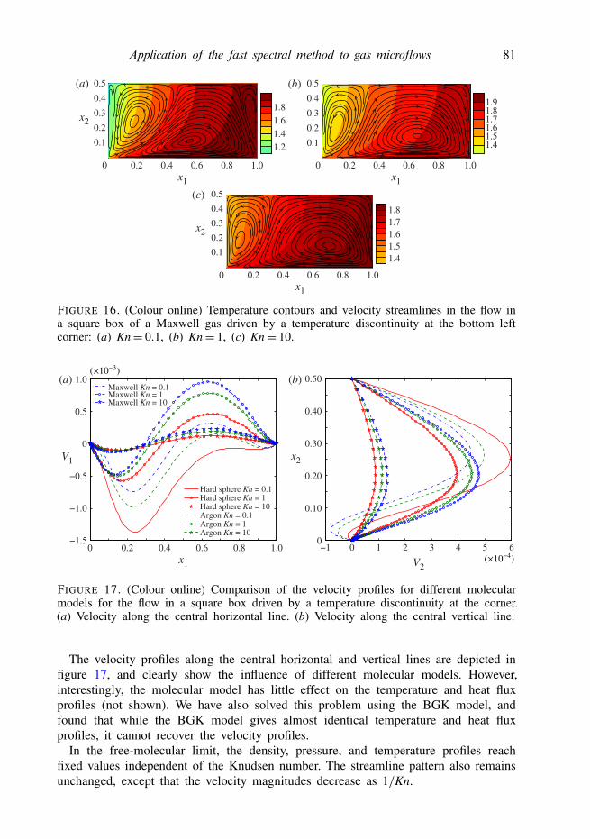
Application of the fast spectral method to gas microflows 81

0 0.2 0.4 0.6 0.8 1.0

0.1

0.2

0.3

0.4

0.5

1.21.41.61.8

(a)

0 0.2 0.4 0.6 0.8 1.0

0.1

0.2

0.3

0.4

0.5

1.41.51.61.71.81.9

(b)

0 0.2 0.4 0.6 0.8 1.0

0.1

0.2

0.3

0.4

0.5

1.41.51.61.71.8

(c)

x1

x1

x2

x2

x1

FIGURE 16. (Colour online) Temperature contours and velocity streamlines in the flow ina square box of a Maxwell gas driven by a temperature discontinuity at the bottom leftcorner: (a) Kn= 0.1, (b) Kn= 1, (c) Kn= 10.

0 0.2 0.4 0.6 0.8 1.0−1.5

−1.0

−0.5

0

0.5

1.0

x2

x1

V1

V2

(a) (b)

−1 0 1 2 3 4 5 60

0.10

0.20

0.30

0.40

0.50

Hard sphere Kn = 0.1Hard sphere Kn = 1Hard sphere Kn = 10Argon Kn = 0.1Argon Kn = 1Argon Kn = 10

Maxwell Kn = 1Maxwell Kn = 10

Maxwell Kn = 0.1

FIGURE 17. (Colour online) Comparison of the velocity profiles for different molecularmodels for the flow in a square box driven by a temperature discontinuity at the corner.(a) Velocity along the central horizontal line. (b) Velocity along the central vertical line.

The velocity profiles along the central horizontal and vertical lines are depicted infigure 17, and clearly show the influence of different molecular models. However,interestingly, the molecular model has little effect on the temperature and heat fluxprofiles (not shown). We have also solved this problem using the BGK model, andfound that while the BGK model gives almost identical temperature and heat fluxprofiles, it cannot recover the velocity profiles.

In the free-molecular limit, the density, pressure, and temperature profiles reachfixed values independent of the Knudsen number. The streamline pattern also remainsunchanged, except that the velocity magnitudes decrease as 1/Kn.

82 L. Wu, J. M. Reese and Y. Zhang

6. ConclusionsWe have studied the application and usefulness of the FSM for gas microflow

simulations. A numerical approximation to both the linearized and nonlinearBoltzmann collision operator was presented. Numerical accuracy has been evaluatedby comparing our FSM results with the numerical kernel method for Poiseuille flow,and excellent agreements in the mass and heat flow rates were seen up to Kn∼ 106.Computational efficiency has been demonstrated on two-dimensional Poiseuille andlid-driven cavity flows, and we found that the FSM can be 10–50 times faster thanthe low-noise DSMC method (which itself is much faster than the original DSMCtechnique for microflow simulations).

We have investigated the influence of different molecular models on the mass andheat flow rates in Poiseuille and thermal creep flows between parallel plates. Themechanism of the variability in flow rates for different molecular models with thesame value of shear viscosity is explained in terms of the effective collision frequency.We also assessed the accuracy of special collision kernels for the LJ potential, andfound that these can produce mass and heat flow rates with a relative error of lessthan 2 % for Kn< 22 and ∼5 % at Kn' 88, when compared to results obtained usingthe realistic LJ potential; for the flow along a rectangular channel, this relative errordecreases as the aspect ratio decreases from infinity to 1.

We have simulated a number of two-dimensional microflows. New insight intoexperimental mass flow rates along a rectangular tube with a large aspect ratio (Ewartet al. 2007) has been provided. We have also analysed quantitatively the influence ofdifferent molecular models on the flow properties. In lid-driven cavity flow, we foundthat the solution is only determined by the value of the shear viscosity, irrespectiveof the molecular model. For thermally driven flows, however, the molecular modelaffects the flow velocity significantly, but the temperature field is not very sensitiveto the molecular model. In the free-molecular regime, our numerical results showedthat the streamline pattern does not change but the velocity magnitudes are inverselyproportional to the Knudsen number. We have also analysed in detail the thermalcreep flow inside a closed rectangular channel, and found that the streamline patterncan be predicted based on the velocity profiles of superposed Poiseuille and thermalcreep flows between parallel plates. These thermally driven flows can serve asbenchmark cases for future investigations.

Finally, we brief analyse why the FSM is suitable for the simulation of moderatelyand/or highly rarefied microflows. The molecular velocity distribution functions havelarge discontinuities at large Kn, hence a significant number of velocity grids areneeded. This poses an extremely difficult problem for other deterministic methodsthat handle binary collisions in velocity space. However, this problem is amenable forthe FSM because the collisions are treated in frequency space. The FSM approximatesthe collision operator with spectral accuracy (Mouhot & Pareschi 2006); the number offrequency components does not need to be as large as the velocity grids. One reasonfor this is that discontinuities in the distribution function produce high-frequencycomponents in its spectrum (and this is usually smooth, or at least smoother than thedistribution function); in the calculation of the spectrum of the collision operator, thespectrum of the distribution function is multiplied by a weight function which is verysmall for high-frequency components (see figure 4 in Wu et al. 2013). Therefore,very high frequencies can be safely ignored: in the transition flow regime, we haveshown that 32 frequency components in each direction is enough.

The only drawback of the FSM, like all other deterministic numerical methods, isthat a large amount of computer memory is required (relative to that required for theDSMC method).

Application of the fast spectral method to gas microflows 83

AcknowledgementsY.Z. thanks the UK’s Royal Academy of Engineering (RAE) and the Leverhulme

Trust for the award of a RAE/Leverhulme Senior Research Fellowship. This workis financially supported by the UK’s Engineering and Physical Sciences ResearchCouncil (EPSRC) under grants EP/I036117/1 and EP/I011927/1. The authors alsothank the reviewers of this paper for their helpful comments.

REFERENCES

BAKER, L. L. & HADJICONSTANTINOU, N. G. 2005 Variance reduction for Monte Carlo solutionsof the Boltzmann equation. Phys. Fluids 17 (5), 051703.

BIRD, G. A. 1994 Molecular Gas Dynamics and the Direct Simulation of Gas Flows. OxfordUniversity Press.

CERCIGNANI, C. 1990 Mathematical Methods in Kinetic Theory. Plenum.CERCIGNANI, C. & DANERI, A. 1963 Flow of a rarefied gas between two parallel plates. J. Appl.

Phys. 34, 3509–3513.CHAPMAN, S. & COWLING, T. G. 1970 The Mathematical Theory of Non-uniform Gases. Cambridge

University Press.DOI, T. 2010 Numerical analysis of the Poiseuille flow and thermal transpiration of a rarefied gas

through a pipe with a rectangular cross-section based on the linearized Boltzmann equationfor a hard-sphere molecular gas. J. Vac. Sci. Technol. A 28, 603–612.

DOI, T. 2012a Effect of weak gravitation on the plane Poiseuille flow of a highly rarefied gas.Z. Angew. Math. Phys. 63, 1091–1102.

DOI, T. 2012b Plane thermal transpiration of a rarefied gas in the presence of gravitation. Vacuum86, 1541–1546.

EWART, T., PERRIER, P., GRAUR, I. A. & MÉOLANS, J. G. 2007 Mass flow rate measurementsin a microchannel, from hydrodynamic to near free molecular regimes. J. Fluid Mech. 584,337–356.

FAN, J. & SHEN, C. 2001 Statistical simulation of low-speed rarefied gas flows. J. Comput. Phys.167, 393–412.

FRANGI, A., GHISI, A. & FREZZOTTI, A. 2007 Analysis of gas flow in MEMS by a deterministic3D BGK kinetic model. Sensor Lett. 6 (1), 1–7.

FUNAGANE, H. & TAKATA, S. 2012 Hagen-Poiseuille and thermal transpiration flows of a highlyrarefied gas through a circular pipe. Fluid Dyn. Res. 44, 055506.

GAMBA, I. M. & THARKABHUSHANAM, S. H. 2009 Spectral-Lagrangian methods for collisionalmodels of non-equilibrium statistical states. J. Comput. Phys. 228 (6), 2012–2036.

GARCIA-COLIN, L. S., VELASCO, R. M. & URIBE, F. J. 2008 Beyond the Navier–Stokes equations:Burnett hydrodynamics. Phys. Rep. 465, 149–189.

GU, X. J. & EMERSON, D. R. 2009 A high-order moment approach for capturing non-equilibriumphenomena in the transition regime. J. Fluid Mech. 636, 177–216.

HOMOLLE, T. M. M. & HADJICONSTANTINOU, N. G. 2007 A low-variance deviational simulationMonte Carlo for the Boltzmann equation. J. Comput. Phys. 226 (2), 2341–2358.

HUANG, J. C., XU, K. & YU, P. B. 2012 A unified gas-kinetic scheme for continuum and rarefiedflows II: multi-dimensional cases. Commun. Comput. Phys. 12, 662–690.

HUANG, J. C., XU, K. & YU, P. B. 2013 A unified gas-kinetic scheme for continuum and rarefiedflows III: microflow simulations. Commun. Comput. Phys. 14, 1147–1173.

JOHN, B., GU, X. J. & EMERSON, D. R. 2010 Investigation of heat and mass transfer in a lid-drivencavity under nonequilibrium flow conditions. Numer. Heat Transfer B 52, 287–303.

JOHN, B., GU, X. J. & EMERSON, D. R. 2011 Effects of incomplete surface accommodation onnon-equilibrium heat transfer in cavity flow: a parallel DSMC study. Comput. Fluids 45,197–201.

LOYALKA, S. K. 1971 Kinetic theory of thermal transpiration and mechanocaloric effect. I. J. Chem.Phys. 55, 4497.

84 L. Wu, J. M. Reese and Y. Zhang

MASTERS, N. D. & YE, W. J. 2007 Octant flux splitting information preservation DSMC methodfor thermally driven flows. J. Comput. Phys. 226 (2), 2044–2062.

MIEUSSENS, L. & STRUCHTRUP, H. 2004 Numerical comparison of Bhatnagar–Gross–Krook modelswith proper Prandtl number. Phys. Fluids 16 (8), 2297–2813.

MOUHOT, C. & PARESCHI, L. 2006 Fast algorithms for computing the Boltzmann collision operator.Maths Comput. 75 (256), 1833–1852.

OHWADA, T., SONE, Y. & AOKI, K 1989 Numerical analysis of the Poiseuille and thermal transpirationflows between two parallel plates on the basis of the Boltzmann equation for hard-spheremolecules. Phys. Fluids A 1, 2042–2049.

PARESCHI, L. & RUSSO, G. 2000 Numerical solution of the Boltzmann equation I: spectrally accurateapproximation of the collision operator. SIAM J. Numer. Anal. 37 (4), 1217–1245.

RADTKE, G. A., HADJICONSTANTINOU, N. G. & WAGNER, W. 2011 Low-noise Monte Carlosimulation of the variable hard sphere gas. Phys. Fluids 23 (3), 030606.

RANA, A., TORRILHON, M. & STRUCHTRUP, H. 2013 A robust numerical method for the R13equations of rarefied gas dynamics: application to lid driven cavity. J. Comput. Phys. 236,169–186.

SHARIPOV, F. 1994a Onsager-Casimir reciprocity relations for open gaseous systems at arbitraryrarefaction. I. General theory for single gas. Physica A 203, 437–456.

SHARIPOV, F. 1994b Onsager–Casimir reciprocity relations for open gaseous systems at arbitraryrarefaction. II. Application of the theory for single gas. Physica A 203, 457–485.

SHARIPOV, F. & BERTOLDO, G. 2009a Numerical solution of the linearized Boltzmann equation foran arbitrary intermolecular potential. J. Comput. Phys. 228, 3345–3357.

SHARIPOV, F. & BERTOLDO, G. 2009b Poiseuille flow and thermal creep based on the Boltzmannequation with the Lennard-Jones potential over a wide range of the Knudsen number. Phys.Fluids 21, 067101.

SHARIPOV, F. & SELEZNEV, V. 1994 Rarefied flow through a long tube at any pressure ratio. J. Vac.Sci. Technol. A 12 (5), 2933–2935.

SHARIPOV, F. & SELEZNEV, V. 1998 Data on internal rarefied gas flows. J. Phys. Chem. Ref. Data27 (3), 657–706.

SHARIPOV, F. & STRAPASSON, J. L. 2012 Ab initio simulation of transport phenomena in rarefiedgases. Phys. Rev. E 86, 031130.

SHARIPOV, F. & STRAPASSON, J. L. 2013 Benchmark problems for mixtures of rarefied gases. I.Couette flow. Phys. Fluids 25, 027101.

SONE, Y. 2002 Kinetic Theory and Fluid Dynamics. Birkhauser.TAKATA, S. 2009a Note on the relation between thermophoresis and slow uniform flow problems

for a rarefied gas. Phys. Fluids 21, 112001.TAKATA, S. 2009b Symmetry of the linearized Boltzmann equation and its application. J. Stat. Phys.

136, 751.TAKATA, S. & FUNAGANE, H. 2011 Poiseuille and thermal transpiration flows of a highly rarefied

gas: over-concentration in the velocity distribution function. J. Fluid Mech. 669, 242–259.VENKATTRAMAN, A. & ALEXEENKO, A. A. 2012 Binary scattering model for Lennard-Jones

potential: transport coefficients and collision integrals for non-equilibrium gas flow simulations.Phys. Fluids 24, 027101.

WU, L., WHITE, C., SCANLON, T. J., REESE, J. M. & ZHANG, Y. H. 2013 Deterministic numericalsolutions of the Boltzmann equation using the fast spectral method. J. Comput. Phys. 250,27–52.