Edinburgh Research Explorer

Experimental study of extracting artificial boundary conditionfrequencies for dynamic model updating

Citation for published version:Hou, C, Mao, L & Lu, Y 2017, 'Experimental study of extracting artificial boundary condition frequencies fordynamic model updating', Smart Structures and Systems, vol. 20, no. 2.https://doi.org/10.12989/sss.2017.20.2.000

Digital Object Identifier (DOI):10.12989/sss.2017.20.2.000

Link:Link to publication record in Edinburgh Research Explorer

Document Version:Peer reviewed version

Published In:Smart Structures and Systems

General rightsCopyright for the publications made accessible via the Edinburgh Research Explorer is retained by the author(s)and / or other copyright owners and it is a condition of accessing these publications that users recognise andabide by the legal requirements associated with these rights.

Take down policyThe University of Edinburgh has made every reasonable effort to ensure that Edinburgh Research Explorercontent complies with UK legislation. If you believe that the public display of this file breaches copyright pleasecontact openaccess@ed.ac.uk providing details, and we will remove access to the work immediately andinvestigate your claim.

Download date: 10. Mar. 2020

1  

Experimental study of extracting artificial boundary condition frequencies for dynamic model updating

Chuanchuan Hou1, Lei Mao2 and Yong Lu1*

1Institute for Infrastructure and Environment, School of Engineering, the University

of Edinburgh, The King”s Buildings, Edinburgh EH9 3JL, UK 2Department of Aeronautical and Automotive Engineering, Loughborough

University, Loughborough, UK

(Received , Revised , Accepted ) Abstract In the field of dynamic measurement and structural damage identification, it is generally known that modal frequencies may be measured with higher accuracy than mode shapes. However, the number of natural frequencies within a measurable range is limited. Accessing additional forms of modal frequencies is thus desirable. The present study is concerned about the extraction of artificial boundary condition (ABC) frequencies from modal testing. The ABC frequencies correspond to the natural frequencies of the structure with a perturbed boundary condition, but they can be extracted from processing the frequency response functions (FRF) measured in a specific configuration from the structure in its existing state without the need of actually altering the physical support condition. This paper presents a comprehensive experimental investigation into the measurability of the ABC frequencies from physical experiments. It covers the testing procedure through modal testing, the data processing and data analysis requirements, and the FRF matrix operations leading to the extraction of the ABC frequencies. Specific sources of measurement errors and their effects on the accuracy of the extracted ABC frequencies are scrutinised. The extracted ABC frequencies are subsequently applied in the damage identification in beams by means of finite element model updating. Results demonstrate that it is possible to extract the first few ABC frequencies from the modal testing for a variety of artificial boundary conditions incorporating one or two virtual pin supports, and the inclusion of ABC frequencies enables the identification of structural damages without the need to involve the mode shape information. Keywords: Damage identification, finite element model updating, modal testing, frequency response function, antiresonance, artificial boundary condition frequencies

                                                            * Corresponding author, Professor, yong.lu@ed.ac.uk

2  

1. Introduction

In structural identification and damage detection, much research has been devoted to developing vibration-based techniques to either perform essentially an inverse procedure to identify structural parameters or construct statistical patterns. The most commonly used vibration data are the natural frequencies, mode shapes, and to a lesser extent damping parameters (Doebling et al. 1996; Sohn et al. 2004; Carden and Fanning 2004). In a physical measurement environment, however, measurement errors and environmental noises dictate that only a limited amount of such data may be obtained with sufficient accuracy.

It is generally recognised that modal frequencies can be measured with higher accuracy than the mode shapes; the errors in the measured natural frequencies may be controlled within 1%, whereas the errors in the mode shape displacements are generally much larger (Mottershead and Friswell 1993; Jones and Turcotte 2002; Fan and Qiao 2011). Moreover, in practice the mode shapes cannot be measured at all DOFs of a system, and this necessitates the mode shape expansion or FE model reduction and such process introduces additional errors. These issues have greatly limited the application of mode shapes or mode shape derivatives in practice (Ratcliffe 1997; Shi and Law 1998; Shi et al. 2000; Qiao et al. 2007).

When it comes to using the natural frequency information for the damage detection, an obvious limitation is by the fact that each natural mode has only one frequency, so the total number of natural frequencies that may be measured from a structure is very limited. Therefore, an enhanced ability to acquire additional modal frequency data is highly desirable in the general damage detection and structural identification field.

In the past, researchers have proposed the use of the zeros (antiresonances) in the frequency response function (FRF) curves as a new type of modal information for damage detection of structures (Lallement and Cogan 1992; Rade and Lallement 1998; Mottershead 1998). Unlike the resonances, zeros occur generally at different frequencies for different measurement points, thus the antiresonance frequencies provide a plentiful resource for the enlargement of the modal data space.

Antiresonances have been employed in FE model updating and damage identification on various types of laboratory structures and proven to be effective. Some of the examples included a steel frame structure and a simplified aircraft beam-assembly called “GARTEUR SM-AG19” benchmark structure (D'Ambrogio and Fregolent 2000, 2003, 2004), a 6m flexible truss structure (Jones and Turcotte 2002), a gas exhaust system and an 8-DOF mass-spring system (Meruane and Heylen 2011, Meruane 2013, Meruane and Mahu 2014), and steel rods and bending vibration beams (Dilena and Morassi 2004, 2009, 2010). Comparisons of updating results with antiresonances and the results with mode shapes indicate that similar accuracy could be achieved. This suggests that antiresonances can serve as an alternative to mode shapes in the finite element model updating.

Theoretically speaking, antiresonances in a particular FRF may be determined from the eigenmode analysis by eliminating a row and a column from both the stiffness and mass matrices of the original system, with the row and column corresponding to the force and response positions of the FRF, respectively (Mottershead 1998). When the row and the column being eliminated are of the same number, i.e., a driving-point FRF case, then the antiresonances are exactly the natural frequencies of the modified system by adding a pin (restraint) to the corresponding DOF.

The above perspective of the driving-point antiresonances is in line with the more general concept of perturbed natural frequencies of a structure, in which case the boundary condition of the structure is to be physically altered (perturbed) so as to generate additional frequency information (Li et al. 1995). The idea of the perturbed boundary condition frequencies, albeit novel, has found

3  

little scope of application because of the obvious impracticality of physically changing the boundary condition of a real structure. The driving-point antiresonances can be seen as a special case of the perturbed natural frequencies in which one single pin support would be added; but by identifying the antiresonances from the driving point FRF, which is measured from the existing structure, the need of physically adding the pin support is avoided.

The possibility of obtaining a diverse range of “perturbed” natural frequencies without the need of physically imposing additional supports has been theoretically established by Gordis (1996, 1999) through the introduction of the concept of artificial boundary condition (ABC) frequencies. Using this approach, the natural frequencies of a structure with “artificially” added (i.e. virtual) pin supports at certain locations may be derived from the incomplete frequency response function (FRF) matrix measured from the existing structure. In the case of one-pin ABC frequencies, the situation degenerates to the driving-point antiresonances (zeros) of the existing structure with a virtual pin added at the driving point. For this reason, and to be consistent with the general ABC frequencies discussed in this paper, hereinafter the driving-point antiresonances will be referred to as “one-pin ABC frequencies”.

With the incorporation of the ABC frequencies, the modal frequency dataset can potentially be expanded drastically. A series of studies has been conducted in this research group to evaluate and enhance the effectiveness of incorporating ABC frequencies in a comprehensive structural identification process and look into the potential issues in extracting ABC frequencies from physical tests (Tu and Lu 2008, Lu and Tu 2008, Mao and Lu 2016). Continued effort is being made to evaluate different experimental aspects of extracting the ABC frequencies, specific measurement error sources, and improve the measurement accuracy, especially for ABC frequencies with more than one pin and in different structural and measurement configurations, as well as the use of such frequencies in structural damage identification.

This paper presents a comprehensive experimental investigation into the extraction of the ABC frequencies in laboratory experiments. Specific error sources in the measured ABC frequencies are discussed and the accuracy of the obtained ABC frequencies is assessed. The extracted experimental ABC frequencies before and after damage are compared to demonstrate the sensitivity of the measured ABC frequencies to damage. FE model updating is then presented in which different sets of the measured modal data, including different combinations of natural modes and/or ABC frequencies, to illustrate the effectiveness of incorporating the ABC frequencies in a practical damage identification application.

2. Overview of basic formulation As mentioned in the Introduction section, modal frequency data for a given structure with added (perturbed) supports provide extended response information which can be used in the structural parameter identification. However, the practicality of such a seemingly attractive idea has been hindered by the fact that imposing added support(s) on a real structure is not normally feasible.

The theoretical work by Gordis (1996, 1999) paved a way for the potential application of the idea of the perturbed boundary frequencies in real structures. In the above publications, it was shown that the natural frequencies of a structure with additional pin supports may be determined by manipulating the frequency response functions measured on the existing structure, without the need to actually impose the additional supports. The perturbed natural frequencies obtained in this way are thus called “artificial boundary condition” frequencies, or in short ABC frequencies herein, to

4  

reflect the fact that the required additional supports are virtual. The theoretical basis of the method is outlined below.

By partitioning between the measured and unmeasured coordinate sets (degrees of freedom, or DOFs), the steady state response of a linear system at a forcing frequency (rad/s) may be written as:

o

m

o

m

ooom

momm2

ooom

momm

f

f

x

x

mm

mm

kk

kk (1)

where, k and m are stiffness and mass matrices, x and f are vectors of generalized response and excitation amplitudes, respectively. Subscript “m” represents measured DOFs and subscript “o” refers to the unmeasured DOFs (“omitted coordinate set” or OCS). The OCS is effectively a reduced system, in which all the measured DOFs are restrained or pinned to the ground.

Introducing the impedance matrix, Z=k-2m, equation (1) can be re-written as:

o

m

o

m

ooom

momm

f

f

x

x

ZZ

ZZ (2)

Assuming no excitations are imposed on the omitted DOFs, i.e., fo=0, from equation (2) we can get:

mom1

oomommm xZZZZf (3)

or

om1

oomomm1

mmm

m ZZZZHx

f (4)

where, Hmm = xm/fm is the measured frequency response function (FRF) matrix containing mm FRF entries (hence incomplete) from the existing structure.

Equation (4) establishes the inherent relationship between the inverse of Hmm and the dynamic characteristics of the OCS as represented by Zoo, such that at the natural frequencies of the OCS, Zoo

-1 is singular, hence Hmm-1 is also singular, and vice versa. Therefore, by identifying the

singularities from the elements of Hmm-1, one can determine the natural frequencies of the OCS, i.e.,

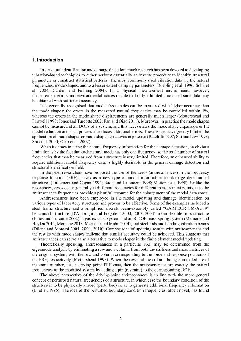
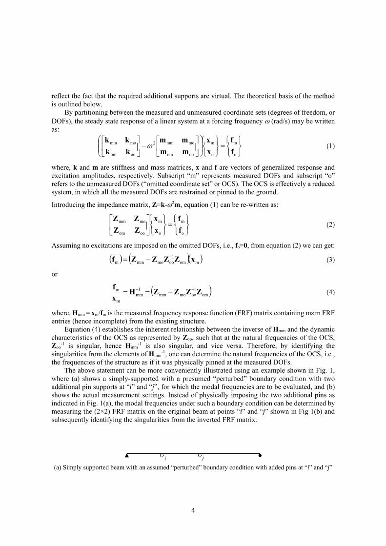
the frequencies of the structure as if it was physically pinned at the measured DOFs. The above statement can be more conveniently illustrated using an example shown in Fig. 1,

where (a) shows a simply-supported with a presumed “perturbed” boundary condition with two additional pin supports at “i” and “j”, for which the modal frequencies are to be evaluated, and (b) shows the actual measurement settings. Instead of physically imposing the two additional pins as indicated in Fig. 1(a), the modal frequencies under such a boundary condition can be determined by measuring the (2×2) FRF matrix on the original beam at points “i” and “j” shown in Fig 1(b) and subsequently identifying the singularities from the inverted FRF matrix.

(a) Simply supported beam with an assumed “perturbed” boundary condition with added pins at “i” and “j”

5  

(b) Artificial boundary condition frequency measurements

Fig. 1 Illustration of artificial boundary condition frequency measurement settings.

3. Experimental investigation of modal testing for ABC frequencies

Previous studies using numerically simulated structures (Tu and Lu 2008) have demonstrated

the effectiveness of incorporating ABC frequencies with one to two pins in the identification of structural parameters and detection of structural damage. The key to bringing the approach of involving ABC frequencies in practical applications rests upon the reliability and accuracy in the acquisition of the ABC frequencies from measured responses. In this section, an experimental exploration on extracting ABC frequencies from physical measurements is presented with a laboratory experiment. Issues and possible improvements with regard to the quality of FRF measurements from an experimental modal testing point of view are highlighted and discussed.

The driving-point antiresonances, i.e. one-pin ABC frequencies as we shall call herein in the context of the present paper, have been actually obtained in modal testing and applied in model updating in the past, as reviewed in the Introduction section. But experimental information on obtaining two-pin ABC frequencies from physical experiments has been scarce. This section aims to discuss the extraction of both one-pin and two-pin ABC frequencies from the experiments.

3.1 Test structure and modal testing program To avoid unnecessary complications from possible structural uncertainties in the experimental study concerned within this paper, the test setup has been kept as simple as possible. The test specimen included steel beams in intact and damaged states. The beams had an identical length of 1020 mm, and a cross-section of width 50 mm and depth 6 mm. The beams were tested under a fixed-end condition, with both ends clamped onto steel supports through bolts and clamping plates, as shown in Fig. 2. The steel supports were considerably stiffer than that of the beam to satisfy the requirement of a fixed support.

6  

(a) Test specimen set-up

(b) Dimensions and test points (Unit: mm)

Fig. 2 Test setup.

In the experiment, an instrumented impact hammer (B&K type 8206-002) was used to excite the test beam. The impact pulse was controlled via using a hammer tip; in the present experiment a plastic tip was found to be suitable to excite the relatively flexible beam. Preliminary tests showed that the hammer was able to generate a flat force spectrum in the range of 0-1000 Hz, which covered comfortably the frequency range of interest for the test beam.

Response of the beam was measured with modal testing accelerometers (B&K Delta Tron® 4508 B 003 type). The accelerometers are light-weight (4.9 g) as compared to the unit segment weight of the test steel beam; therefore the influence of transducer mass on modal testing results was negligible. Because the driving point FRF curves are required as part of the FRF matrix in order to determine the ABC frequencies, all accelerometers were attached to the bottom side of the steel beam (Fig. 2(a)). During the experiment, a measurement array was arranged by dividing the beam length along the centreline into a number of segments, herein 10 segments were considered, giving rise to 9 measurement points (excluding the two end supports), as shown in Fig. 2(b).

For simplicity and without losing generality, the experimental study was focused on two-pin ABC frequencies, in addition to the simpler one-pin ABC frequencies. As a matter of fact, with just one and two-pin supports a large number of variations in the support locations can already be configured, providing a range of ABC frequency combinations. It is also worth noting that the extraction of ABC frequencies involves inversion of the incomplete FRF matrix whose dimension increases with the number of the artificial pins, therefore using more than 2-pins would introduce increased complexity in the influence of the measurement errors. To facilitate the measurements for all one- and two-pin configurations, two accelerometers are required and these were attached to two measurement points (i and j) at any one time, as illustrated earlier in Fig. 1.

The impact force and acceleration response signals were acquired with a multi-channel data acquisition module. Because the detailed FRFs are needed to generate the ABC frequency function curves, it was essential that the impact force time history was captured with high accuracy; otherwise

7  

spurious peaks could occur on the FRFs. Since the impact force lasts for a very short duration, typically in a fraction of a millisecond (see Fig. 3(a)), a high sampling rate of above 10 kHz was required. After trial testing and data analysis with different sampling rates, it was found that sampling at 25.6 kHz was appropriate in that the resulting FRF curves were smooth enough and further increase of the sampling rate had no noticeable effect. This sampling rate was therefore employed for both input and output signals during the tests. One further requirement for transient modal testing is that the response signals of the structure should be fully recorded to avoid leakage in modal analysis (Ewins 1984). To this end, a record duration was set at 16 s, which proved to be adequate to both cover the useful signal and maintain a manageable data size. Representative input force and output acceleration signals obtained from the tests are shown in Fig. 3.

(a) Impact force (Zoomed) (b) Acceleration

Fig. 3 Representative recorded impact force and acceleration signals.

Three different groups of tests were carried out to obtain the natural modes, one-pin ABC frequencies and two-pin ABC frequencies, respectively. More details follow.

(1) The first test was to obtain natural frequencies as well as mode shapes of the beam. As mentioned earlier the beam was evenly divided into 10 segments, resulting in 9 measurement points along the beam length. To obtain the mode shapes, a complete row or column of the FRF matrix needs to be measured. In the present test the response measurement location was fixed while the impact location moved from point to point. To avoid nodal point in any of the first few mode shapes an accelerometer was fixed at location P7 (Fig. 2), and 9 different measurements with excitation at each of the 9 measurement points, respectively, were carried out.

(2) One-pin ABC frequencies can be obtained from the driving point FRF curves. As representation, three driving points (or ABC pin locations) at P4, P7 and P8, respectively, were tested.

(3) Two-pin ABC frequencies involve two virtual pin locations. Again as representation, three two-pin configurations were chosen in the tests, with pins at (P2, P5), (P4, P7) and (P4, P8), respectively. For each configuration, two accelerometers were attached at the virtual pin locations and the excitation was imposed at each of the two locations in turn. Referring to Fig. 1 again, to measure the FRFs for the two-pin ABC frequencies with the two virtual pins at locations (i, j), the excitation (impact) is firstly applied at location i while the responses are measured at both i and j, yielding FRFii and FRFij. Subsequently the excitation is applied at j while the responses are measured again at i and j, yielding FRFji and FRFjj. Thus, four FRF curves are obtained, including two driving-point FRFs and two transfer FRFs. This completes the measurement for the two-pin ABC

-30

0

30

60

90

120

150

0.977 0.978 0.979 0.98 0.981 0.982

For

ce/N

t/s

-200

-100

0

100

200

0 4 8 12 16

Acc

eler

atio

n/m

/s2

t/s

8  

configuration of (i, j). The same procedure was repeated for all selected two-pin ABC configurations. Note that in the current tests both the one-pin and two-pin ABC configurations (locations of the pins) were randomly chosen.

The FRF curves are calculated by the following equation:

)(

)()(

F

XH (5)

where, X() is the Fourier transform of the output signal and F() is the Fourier transform of the input signal, H() is the measured FRF curve.

From the definition explained in the Basic Formulation section, the two-pin ABC frequency function curves can be calculated as:

1

jjji

ijii

jjji

ijii

HH

HH

AA

AA (6)

where, Aij (i, j=1, 2) are the elements of the inverse of the incomplete FRF matrix, which effectively form the two-pin ABC frequency function curves with the resonance in each of these functions being the ABC frequencies. Hereinafter Aij will be referred to simply as ABC frequency function.

In obtaining the measured FRF curves, standard force windowing is applied on the impact force curve and a rectangular window with the same duration as the impact force is used. 5 repetitive tests were performed to allow for an average on the resulting FRF curves.

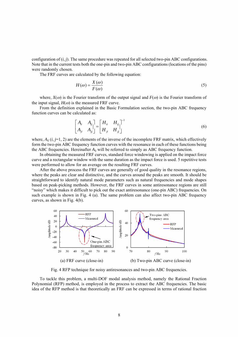
After the above process the FRF curves are generally of good quality in the resonance regions, where the peaks are clear and distinctive, and the curves around the peaks are smooth. It should be straightforward to identify natural mode parameters such as natural frequencies and mode shapes based on peak-picking methods. However, the FRF curves in some antiresonance regions are still “noisy” which makes it difficult to pick out the exact antiresonance (one-pin ABC) frequencies. On such example is shown in Fig. 4 (a). The same problem can also affect two-pin ABC frequency curves, as shown in Fig. 4(b).

(a) FRF curve (close-in) (b) Two-pin ABC curve (close-in)

Fig. 4 RFP technique for noisy antiresonances and two-pin ABC frequencies.

To tackle this problem, a multi-DOF modal analysis method, namely the Rational Fraction Polynomial (RFP) method, is employed in the process to extract the ABC frequencies. The basic idea of the RFP method is that theoretically an FRF can be expressed in terms of rational fraction

9  

polynomials. With numerical manipulations on a measured FRF curve, the coefficients of the polynomials can be obtained. The actual modal parameters can then be extracted from the polynomial form of the FRF curve. Richardson and Formenti (1982) employed orthogonal polynomials in the RFP method and made it suitable for computer-based calculation. The RFP method is employed here to obtain ABC frequencies which would otherwise be difficult to determine with the peak-picking method due to noise in the curves. To obtain one-pin ABC frequencies, RFP is applied on the FRF curves directly. But when obtaining the two-pin ABC frequencies, RFP is applied on the ABC frequency function curves instead of the original FRF curves.

The effect of RFP on FRF curves and ABC frequency function curves is shown in Fig. 4 in which the original measured data are labelled as “Measured” and the RFP-processed data are labelled as “RFP”. It can be seen that the processed FRF and ABC frequency function curves from using RFP match quite well the measured curves overall, and at the same time the valleys, as well as peaks, are cleared up, paving the way for the extraction of the ABC frequencies from the RFP curves.  

Fig. 5 presents representative driving FRF and ABC frequency function curve for a two-pin scenario in a combined plot. The natural (resonance) frequencies, one-pin ABC (antiresonance) frequencies, as well as two-pin ABC frequencies are marked respectively. While one-pin ABC frequencies are simply driving-point antiresoannce and hence are subject to the same measruement constraints as antiresoannces, it can be observed clearly that the two-pin ABC frequencies are generally not associated with the antiresonances. Recall the theoretical background presented in Section 2; the multi-pin ABC frequency curves are constructed from inverting the measured FRF matrix (for two-pin ABC here this is 22 matrix), and as a result the peaks on the inverted matrix elements have no direct connection to either antiresonance frequencies or the resonances in an individual FRF.

Fig. 5 Representative driving FRF and two-pin ABC frequency function curves.

3.2 Modal testing results

The implementation of the above mentioned data processing procedure proved to work well in this experiment towards generating the ABC frequencies. From Fig. 5 it can be seen that both the FRF curve and ABC frequency function curve exhibit satisfactory quality; the noise level in the curves is relatively low, and resonances and antiresonances can be clearly identified from the FRF

-60

-40

-20

0

20

40

60

0 100 200 300 400 500

Am

plit

ude/

dB

f/Hz

FRFABC

Natural

One-pin

Two-pin

10  

curve as well as the two-pin ABC frequency function curve. With the basic peak-picking, deep-picking methods and RFP technique, the natural frequencies, mode shapes and ABC frequencies can now be obtained conveniently.

Table 1. Measured and predicted natural and one-pin ABC frequencies (Unit: Hz).

Mode Natural frequency One-pin at P4 One-pin at P7 One-pin at P8

f0Nm f0Nc /% f0Am f0Ac /% f0Am f0Ac /% f0Am f0Ac /%

1 28.9 29.0 0.1 66.8 66.2 0.8 52.6 51.4 2.2 41.4 41.2 0.5 2 79.9 79.9 0.0 145.8 145.8 0.0 146.0 143.6 1.7 117.3 115.0 1.9 3 157.0 156.6 0.2 211.9 210.1 0.8 247.3 251.8 1.8 231.0 227.1 1.7 4 259.2 259.2 0.0 385.1 386.2 0.3 322.6 321.0 0.5 380.6 375.8 1.3 5 387.3 388.3 0.3 - - - - - - - - - Mean 0.1 0.5 1.5 1.3

Table 2. Measured and predicted two-pin ABC frequencies (Unit: Hz).

Mode Pins at P2 and P5 Pins at P4 and P7 Pins at P4 and P8

f0Am f0Ac /% f0Am f0Ac /% f0Am f0Ac /%

1 95.6 95.4 0.2 139.8 138.6 0.9 116.5 113.5 2.6 2 218.6 212.2 2.9 211.4 209.2 1.1 172.5 169.7 1.6 3 305.9 303.9 0.7 298.2 299.5 0.5 376.1 369.1 1.8 4 533.9 542.0 1.5 452.4 452.3 0.0 471.6 471.8 0.0 Mean 1.3 0.6 1.5

Tables 1 and 2 summarize the measured natural frequencies and one-pin and two-pin ABC frequencies of the intact steel beam. In the tables, “fN” represents natural frequencies and “fA” represents ABC frequencies. Subscript “0” indicates the beam is intact, subscript “m” denotes measured data while subscript “c” denotes predicted data. The predicted data are from calibrated finite element model of the beam, which will be discussed slightly later.

Fig. 6 Displacement-normalized mode shapes.

-1

-0.5

0

0.5

1

0 102 204 306 408 510 612 714 816 918 1020

Mod

e sh

ape

x/mm

1st mode2nd mode

11  

Fig. 6 illustrates the first two displacement-normalized mode shapes. In all, the first 5 natural modes, including natural frequencies and mode shape displacements at the measured locations could be obtained from the tests. On the other hand, the first 4 ABC mode frequencies for each of the two-pin configuration can be determined from the tests without ambiguity.

4. Discussion on the measurement accuracy of ABC frequencies

The previous section has established that the first few (4 herein) ABC mode frequencies are obtainable from a standard modal testing and data processing procedure. This section examines the accuracy in the measured ABC frequencies in terms of the susceptibility of these frequencies to some common variability in conducting the physical tests, such as the actual impact location.

It is generally believed that antiresonances will have similar measurement accuracy as resonances (D'Ambrogio and Fregolent 2000, 2003), and as such when these data are employed in a parameter identification (model updating) process, uniform weighting is generally used regardless resonances or antiresonances (D'Ambrogio and Fregolent 2000; Meruane and Heylen 2011). Non-uniform weighting for resonances and antiresonances has also been considered; for example Jones and Turcotte (2002) assigned different weighting factors for resonances and antiresonances based on the assumption that the coefficient of variance of antiresonances is 2 times of that of resonances. However, in the context of the general ABC frequencies with more than one pin, there is a lack of analysis on the accuracy of the measured ABC frequencies from a modal testing procedure.

Natural frequencies and ABC frequencies share the same character in that they both are associated with the peaks on the FRF curve or ABC frequency function curve, respectively. However there exist fundamental differences between the two types of frequencies. While the natural frequencies are independent of the excitation and response measurement locations, the ABC frequencies depend closely upon the locations of excitation and response. This characteristic is similar to the well-known location-dependent characteristic of the antiresonances, which in the driving-point case are simply a special case of the ABC. As a consequence, any imprecision in the excitation and measurement locations could bring errors into the ABC frequencies.

The following error sources are examined here; (1) errors due to misalignment of the excitation location and the sensor location, (2) errors due to sensor mass, and (3) additive noise.

4.1 Errors pertaining to imprecise excitation location Input location error could arise from the limitation of modal testing setup or manual operation. For example, one-pin ABC frequencies are obtained from driving antiresonances. To get driving FRF curves, we need the input excitation and the output response measurement locations in the structure to be identical. However this is hard to achieve in practice. Usually there are three alternative options to deal with driving point measurements (Ewins 1984). The first one is to use an impedance head which can measure both the impact force and excitation response at a single point. The second one is to place the sensor alongside but as close as possible to the excitation point, as shown in Fig. 7. As the excitation location is actually shifted from the theoretical target point, the ABC frequencies will be affected. The third option may be suitable for thin structure such as the steel beam tested herein, and in this approach the impact and the output sensor are placed in line but on opposite sides of the structure. However there is still no 100% guarantee of achieving the exact alignment, especially when the excitation (e.g. an impact hammer) is handled manually. For these reasons, a

12  

detailed examination of the sensitivity of the one-pin and two-pin ABC frequencies to the misalignment of the impact and output response locations is deemed to be instructive.

The scenario is illustrated in Fig. 7. The target driving FRF is at point i, Hii, and the sensor is placed at i. Assuming the impact point is offset by a distance of d, at point i′. We shall examine the sensitivity of ABC frequencies to d.

Fig. 7 Modal testing operation when obtaining one-pin ABC frequencies.

The sensitivity of antiresonances from an FRF curve Hkj to parameter p has been given in Mottershead (1998), which is a linear combination of sensitivities of eigenvalues and eigenvectors. It is convenient to get an explicit sensitivity relationship for driving function Hii, i.e. one-pin ABC frequencies fA. If we take d as a structural parameter, and consider that eigenvalues will not change with d because they are global parameters and do not depend on the excitation location, we can get the sensitivity of fA

2 to d, as:

N

kik

N

kpp

pkik

N

kikk

ik

f

fd

d

f

1 1,

2A

1

2A2

A

det

det

IΛ

IΛ (7)

where, = diag(n), n=1, 2, …, N, andk is the nth eigenvalue; the subscripts k, p on the matrix (-fA

2I) mean that the kth and pth rows and columns have been deleted. ∂ik is the change of mode shape element ik due to the change of excitation location; in the example considered here,

ikkiik (8)

It is actually the difference of the mode shape elements at point i′ and i. It is clear from equation (7) that the sensitivity of fA

2 is a linear combination of the sensitivities of the mode shape element at point i from different modes. In other words, the error brought by the location misalignment in the one-pin ABC frequency is a linear combination of shifts in the mode shape element at the driving point due to the misalignment. The same procedure can be applied on two-pin ABC frequencies. From equation (6), the two pin ABC frequencies are actually frequency points which satisfy:

0 jiijjjii HHHH (9)

13  

In the two-pin situation, the excitation location errors involve two contributions, one from the actual point i′, which is d1 away from point i, and one from the actual point j′, which is d2 away from point j. So the measured two-pin ABC frequencies manifest as satisfying:

0 ijjijjii HHHH (10)

The FRF curves can be expressed in terms of the eigenmode data (Mottershead14), as:

N

k k

jkikijH

12

(11)

With equation (10) and (11), the two-pin ABC frequencies fA can be determined from:

0det1 1

,2

A

N

p

N

pqq

qpiqjpjqippjpi f IΛ (12)

The sensitivity of fA2 to d1 and d2 can be calculated following a similar approach as the

ansiresonance sensitivity:

11

1 1,

1,,

2A

1,

2A

1

2A

det

det

df

f

d

f ipN

p N

p

N

pqq

N

qpmm

mqpjpiqjqipjqip

N

pqq

qpjpiqjqipjq

IΛ

IΛ

(13a)

21

1 1,

1,,

2A

1,

2A

2

2A

det

det

df

f

d

f jqN

q N

p

N

pqq

N

qpmm

mqpjpiqjqipjqip

N

qpp

pqjpiqjqipip

IΛ

IΛ

(13b)

Thus the shift of a two-pin ABC frequency fA due to the location errors can be calculated as:

22

2A

11

2A2

A ddd

fdd

d

fdf

(13c)

Equation (13) showed that, similar to one-pin ABC frequencies, the error brought by the location misalignment in two-pin ABC frequencies is also a linear combination of shifts of the mode shape displacements at the two virtual pin locations.

14  

Considering that the offset distance d can be controlled within a reasonably small range, with an upper limit of the order of the size of the sensor (when placed on the same side of the impact strike), it can be assumed that the mode shape variation within this range is linear. On this basis, and using the expressions in equation (7) and (13), it can be demonstrated that the relationship between the error in ABC frequencies and d, d1 or d2 are approximately linear. Such relationship has also been confirmed with FEA analysis, which is not presented here for the sake of space. This property leads to a proposed testing operation for the measurement of ABC frequencies in terms of mitigating the location errors, which can be stated as follows. a) Generally speaking, a sufficient number of repeated tests should be performed with the impact being imposed around the target location in a random manner, and the obtained ABC frequencies (squared) should be averaged in order to cancel out the errors due to the location misalignment. b) When the sensor and impact need to be applied on the same side of the structure (as would be the case for civil engineering structures), such that the precise location is occupied by the sensor, repetitive tests should be performed with the impact being applied on both sides of the sensor, and average of the resulting ABC frequencies (squared) should be taken. 4.2 Errors pertaining to the sensor mass

It is well known that the testing devices attached to the structure, such as a sensor or a shaker stinger, will alter the dynamic properties of the tested structure itself to a certain extent due to the presence of an additional mass. Several studies have been conducted to find ways to cancel out the mass effect of sensors (Ashory 2001). As far as antiresonances and ABC frequencies are concerned, however, these frequencies can be deemed as immune to the effect of a sensor mass so long as sensors are only attached at the “pin” positions. This is because ABC frequencies are by virtue the natural frequencies of the structure with the measured nodes being “pinned”. Consequently there should be no vibration in the ABC system at the locations of the sensors.

4.3 Errors pertaining to additive noise

It is generally known that the commonly used FRF curve estimators H1 and H2 are biased to the uncorrelated additive noise, as shown in equation (14) (He and Fu35).

)()()(

)(1)(

)(ˆ)(ˆ

ˆ1

1

FF

MM

FF

XF1

H

S

SH

S

SH

(14a)

)()()(

)(1)(

)(ˆ)(ˆ

ˆ2

XX

NN

XF

XX2

H

S

SH

S

SH

(14b)

where, “F” stands for the excitation force; “M” stands for the additive noise in the excitation force; “X” stands for the output response; “N” stands for the additive noise in the output response. S() is the auto- or cross- spectrum of the signals. H() is the real value of FRF curves. The symbol “^” indicates the term is an estimator.

It is clear from equation (14) that the amplitude of the FRF curves will be biased when additive noise is present. For the extraction of one-pin ABC frequencies, as the quality of FRF curve around the antiresonant area is of main concern, H1 should be a better estimator over H2 due to the fact that

15  

the response of the structure is quite insignificant at antiresonances and 2 is relative large. If the spectrum of the force is generally smooth and 1 does not have a large variation around the antiresonances, the extracted one-pin ABC frequencies can be seen as unbiased. This is due to the fact that the antiresonances are obtained from the frequency axes of the FRF curves rather than the amplitude axes. So as long as 1 does not present a large variation, the location of the peak on the frequency axes would not change even though the amplitude might be biased.

When H1 or H2 are used as the estimator of FRF, the two-pin ABC frequencies calculated with equation (9) can be written as:

0ˆˆˆˆ jiijjiijjjiijjiijiijjjii HHaaHHaaHHHH (15)

In modal testing, we use the same excitation force to obtain FRFii and FRFij (Excitation at point i), and the same excitation force to obtain FRFji and FRFjj (Excitation at point j). As a result, when H1 is used as the estimator, we will have ii=ij, ji=jj. We can see from equation (15) that the two-pin ABC frequencies from the FRF estimators will be unbiased to the values from real FRF curves. When H2 is used as the estimator, from equation (14b) we can see that the coefficient 2 will depend on the SNR (signal-to-noise ratio) of the response. As the SNR could be different for the four responses, the obtained two-pin ABC frequencies could be biased, especially when the driving and transfer FRF curves have distinctive SNRs. From this point of view, H1 should also be a better choice under such conditions.

From the above analysis on the effects of a few common error sources, it can be argued that the measured ABC frequencies are generally unbiased to such errors, and through properly designed modal testing and signal processing strategies the influence of these errors can be minimised. We can therefore postulate that the measurement of ABC frequencies can achieve similar accuracy as that of the natural frequencies. In the next section, we shall examine the accuracy in the measured ABC frequencies from the experiment against the predicted results from a calibrated (updated) finite element model.

4.4 Verification of accuracy of extracted ABC frequencies from test data

The ABC frequencies generated from the experimental data are verified against numerically simulated ABC frequencies from a carefully calibrated FE model to evaluate their accuracy. Once a finite element model is calibrated to a satisfactory degree, the computation of the ABC frequencies is straightforward as these frequencies are simply the natural frequencies of the structure when the artificial pin constraints are physically imposed, and this can be done easily with the FE model. However, the FE model should be accurate enough to represent the test beam, and to this end a calibration updating of the basic properties of the FE model needs to be carried out beforehand.

To be consistent with the measurement arrangement in the experiment, in the FE model the beam is discretised into 10 elements, corresponding to the 10 segments in the test. To compensate the coarse discretisation and to take into account the shear deformation and rotational inertia, high order (cubic) Timoshenko beam elements are used to establish the FE model and this ensures a minimal modelling error. The boundary conditions of the beam model follow the experiment and are fixed. The density and Poisson”s ratio of the material are known constants for the steel material and are 7850 kg/m3 and 0.3, respectively. The bending stiffness as represented by the beam flexural rigidity EI is unknown and needs to be identified (updated). Since the intact beam is highly uniform, a single flexural rigidity value is updated from the FE model updating.

16  

For the updating of a single variable, we choose to employ only the natural frequencies as these data are deemed to have the highest measurement accuracy. The first five natural frequencies as available from the experiment are employed and accordingly the objective function, which is to be minimised in the updating process, is formed as follows:

5

12Nm0

2Nm0

2Nc0abs

i i

ii

f

ffJ (16)

where, f0Nmi and f0Nci stand for the measured and calculated ith natural frequencies of the intact beam. The parameter EI in the beam model is iteratively adjusted to achieve minimum of the objective

function J. The result for EI is 168.9 N·m2. A comparison between the measured natural frequencies and the computed ones using the above property is given in Table 1. It can be seen that the results match very well.

The updated FE model is then employed to compute the one-pin and two-pin ABC frequencies in a forward manner (adding actual pin(s)). The results are presented in Tables 1 and 2, in which the relative differences between the measured and predicted frequencies are also included (the term in percent).

It can be seen that the measured and predicted ABC frequencies match quite well with each other. The average error is less than 1.5%, which is about the order that is generally known to the measurement of the natural frequencies. It is worth noting that the error in the natural frequencies shown in Table 1 is considerably small (average about 0.1%) in the present case, and this is attributable to the fact that the FE model has been calibrated against these measured natural frequencies, therefore a near zero difference between the measured and predicted values is expected and this may not be directly comparable with the differences in the subsequently calculated ABC frequencies.

From the above verification against the predicted results, it can be concluded that both one-pin and two-pin ABC frequencies can be measured with good accuracy from actual experiment.

5. Extracting ABC frequencies from damaged beams and damage identification The last two sections have demonstrated that good quality one-pin and two-pin ABC frequencies can be obtained from modal testing in a physical measurement environment and the accuracy of the measured ABC frequencies is similar to the generally recognised measurement accuracy of the natural frequencies. In this section the effectiveness of employing ABC frequencies in the damage identification is evaluated with comparison to the use of conventional modal data. 5.1 Test specimens and modal testing results Two steel beams with the same properties as the one reported in Fig. 2, but with the introduction of damages, were tested under the same procedure. The damages were intended to represent a realistic scenario where identification using a global method with modal data could be possible. To this end, the damages were created in the beam by making several cuts within a limited length to simulate a sensible reduction of the flexural rigidity over the area, as shown in Fig. 8. In the first beam, denoted as B1, the cuts were spread slightly less than a segment length, in the area between 300 mm to 400 mm from the left support. The saw cuts were made with a width of 1 mm and depth of 12.5 mm,

17  

and the interval between the cuts was 10 mm. The damage area was located between the points P3 and P4 shown in Fig. 2. The resulting stiffness reduction as equivalent over a whole segment was about 40%. The second beam, denoted as B2, had exactly the same pattern of cuts located between points P3 and P4, but it had a second damage area between points P7 and P8 with cuts spreading over half of the segment length. Therefore, the first beam effectively represented a scenario with a single damage zone, whereas the second beam represented a scenario with multiple damaged zones.

Fig. 8 Damages in steel beams.

Table 3. Measured natural and ABC frequencies of damaged beams (Unit: Hz).

Mode Natural frequency (fdNm)

One-pin at P4 (fdAm)

One-pin at P7 (fdAm)

Two-pin at P4 and P7 (fdAm)

Beam B1 Beam B2 Beam B1 Beam B2 Beam B1 Beam B2 Beam B1 Beam B2 1 28.4 28.3 65.2 62.6 49.7 46.5 137.8 137.1 2 77.1 74.3 142.9 142.9 144.4 142.1 203.4 200.5 3 156.6 153.3 205.3 201.3 243.3 242.3 295.9 286.4 4 248.6 248.5 385.1 368.6 49.7 301.9 433.7 433.9 5 377.9 370.0 - - - - - -

The modal testing procedure was applied on the two damaged beams and the same types of

modal data, including the first 5 modes of natural frequencies and mode shapes and the first 4 modes of one-pin and two-pin ABC frequencies from selected configurations, were obtained. The measured natural frequencies and selected ABC frequencies are listed in Table 3. In the table, the subscript “d” denotes damaged beams. Comparing with Table 1 and 2, it shows that the damages will bring a decrease of 0.3-5% to natural and ABC frequencies of beam B1 and a decrease of 2-11% to those of beam B2.

5.2 Damage identification through FE model updating

The measured modal data are employed to do damage identification through FE model updating

for the two damaged beams. To evaluate the effectiveness of different types of the modal data in the FE model updating, a comparative study is carried out with different combinations of the dataset to include natural frequencies, one-pin or two-pin ABC frequencies, and mode shapes, separately or in a mixed fashion.

Different objective functions are formed in accordance with different types of modal data employed, and parallel updating procedures are performed with different objective functions to compare the outcome. The objective functions are established with the residuals of the modal data.

18  

In what follows, different types of residuals are described first, and the objective functions combining different residuals and hence different combinations of the modal data are presented next.

(1) Residual from natural frequencies

The residual from natural frequencies is defined as Rf in equation (17a). It gauges the difference between theoretical (from FE model) and measured frequencies for the damaged beam. To minimise the influence of the model error, the measured and theoretical natural frequencies for the damaged beam are normalised with respect to their undamaged counterparts, and the residual is formulated from the normalised values:

f

12Nc0

2dNc

2Nm0

2dNm

ff abs

1 N

i i

i

i

i

f

f

f

f

NR (17a)

where, fNi represents the ith natural frequency; subscripts “c” and “m” stand for the FE calculated and the measured data, respectively; and subscripts “d” and “0” stand for the damaged and intact states of the beam, respectively. Nf is the number of modes used.

(2) Residual from ABC frequencies (one-pin or two-pin)

A similar form of residual, defined as RA, is formed for one-pin and/or two-pin ABC frequencies:

A

12Ac0

2dAc

2Am0

2dAm

AA abs

1 N

i i

i

i

i

f

f

f

f

NR (17b)

where, fAi represents the ith mode of ABC frequency (one-pin or two-pin). NA is the number of ABC modes used.

(3) Residual from Modal Assurance Criterion (MAC)

Mode shapes may be applied to form the residual by directly using the mode shape changes or mode shape derivative changes. Residuals from these two different types of data might provide different results for model updating, so both methods are employed in the updating analysis here.

Firstly the widely used mode shape derivative, Modal Assurance Criterion (MAC), is used here to gauge the effect of damage from the perspective of the mode shapes, and this is defined as:

iiii

iii

dTd0

T0

2

dT0MAC

(17c)

where, i stands for the ith mode shape vector of the beam; subscripts “0” and “d” stand for mode shapes of the intact and damaged beam, respectively.

The residual is then formed by taking into account the difference between the measured and predicted MAC values of the first NMAC modes, as:

MAC

1

2cm

MACMAC MACMAC

1 N

iiiN

R (17d)

19  

where, subscripts “c” and “m” stand for the FE calculated and measured MAC values, respectively.

(4) Residual from mode shape changes

As mentioned, the residual can also be directly formed from mode shape changes, as shown in equation (17e). The first NMS modes of mode shapes are used in the formula. To make the mode shape displacements comparable, both the measured and predicted mode shapes are displacement-normalized.

MS N

1 1

dc

dm

NMSMS abs

1 N

i

N

jjijiNN

R (17e)

where, ji is the jth element in the ith displacement-normalized mode shape vector. The superscript “d” stands for damaged beam and NN is the total number of elements in each mode shape vector, which is 9 in the current measurements.

The objective functions can then be formed with different combinations of the above residuals. Five different types of objective functions are used in the comparative study, as listed below. In all of the objective functions, unit weights were applied to different types of modal data in the study here.

The first objective function is formed only with natural frequencies to serve as a reference for the other ones, as shown in equation (18a). The first five modes of natural frequencies are used in J1.

f1 RJ (18a)

One-pin ABC frequencies are added in J1 to form the second objective function J2, as shown in equation (18b). The numbers in the subscript denote the “pin” locations. In each configuration, the first three modes of one-pin ABC frequencies are used, making the total number of one-pin ABC frequencies involved in the objective function to be 9.

A8A7A4f2 RRRRJ (18b)

Two-pin ABC frequencies are added to J1 to form the third objective function J3, as shown in equation (18c). Similar to equation (18b), the numbers in the subscript denote the “pin” locations and the first three modes of two-pin ABC frequencies are used for each configuration. Similar to J2, the total number of two-pin ABC frequencies involved in J3 is also 9.

A48A47A25f3 RRRRJ (18c)

The fourth objective function J4 is formed by adding the MAC residual to J1, as shown in equation (18d). Considering that in modal testing practice generally only the first couple of mode shapes may be measured with reliable accuracy, the first two mode shapes are used in this objective function.

MACf4 RRJ (18d)

The fifth objective function J5 is formed by adding the mode shape change residual to J1, as shown in equation (18e). Similar to J4, the first two modes are used in J5.

20  

MSf5 RRJ (18e)

5.3 Model updating considerations

An FE model with 10 Timoshenko beam elements is used to model the damaged beams. Herein the damage is modelled as a reduction of the element stiffness for a beam element. A stiffness reduction ratio Di is defined for the ith element in the model by the following expression:

0d 1 KK ii D (19)

where, K0 and Kd are the stiffness matrix of the intact and damaged beam element, respectively. In the model updating, for generality each element in the beam model is assumed to have an

unknown damage state which need to be updated. So totally there are 10 parameters to be updated, i.e., Di, i=1, 2, …, 10.

For the search of the damage parameters the Genetic algorithm (GA) is employed. GA has been used widely as an optimization tool in engineering applications (Perera and Torres 2006). Compared with using traditional methods, GA-based model updating has several advantages. For example, the GA searching results do not depend on the initial setting of the updating parameters, thus a global optimal result rather than a local one is generally guaranteed. Furthermore, because the variable parameters are gradually optimized through an evolutionary algorithm, it does not involve the calculation of the sensitivity matrix of the structure, and this makes the updating process more robust. There have been many successful applications of using GA in model updating problem, some of which are summarized in Perera and Torres (2006). In the present study, the standard GA function in Matlab has been used to update the FE model. The convergence process of the GA calculation is monitored and it is found that a limit of maximum generation of 1500 is adequate to achieve satisfactory converging result in the present FE model updating applications.

5.4 FE model updating (damage identification) results Five parallel updating procedures with five different objective functions listed in equation (18a-

e) are carried out for the two damaged beams separately. The updating results are presented in Fig. 9-13. In beam B1, the damaged element should be the 4th element, while in beam B2 the damaged elements should be the 4th and 8th elements. The equivalent element stiffness changes in the damage segments of the test beams were approximately 40% and 25% respectively, according to the cuts. This means the expected damage index Di would be about 0.4 in element 4 for beam B1, and 0.4 in element 4 and 0.25 in element 8 for beam B2. The rest of the elements should have a D value being virtually zero (undamaged).

It can be seen that when only the lowest five modes of natural frequencies are used in the updating (J1, Fig. 9), the correct damage element cannot be identified for beam B1, whereas in beam B2, a false crack is identified in the 7th element. The first reason for the failed updating is that natural frequencies are global scalar properties and cannot resolve the symmetry problem in terms of the damage location. As seen from the result for beam B1, the real damage should be in the 4th element but the identified damage is in the symmetric element along the beam span. Another reason here is that the number of unknown parameters (being updated) is larger than that of the input data, therefore

21  

it is an under-determined problem and consequently false identification of damages, such as the situation in beam B2, is basically inevitable.

Fig. 9 Updating results with J1. Left: Beam B1; Right: Beam B2.

Fig. 10 Updating results with J2. Left: Beam B1; Right: Beam B2.

 

Fig. 11 Updating results with J3. Left: Beam B1; Right: Beam B2.

When one-pin ABC frequencies are added into the objective function (J2, Fig. 10), it is found that the above issues are readily avoided and correct damage elements can be identified in both beam B1 and B2. Even better results are obtained when two-pin ABC frequencies are joined with the natural frequencies (J3, Fig. 11). These outcomes demonstrate that both one-pin and two-pin ABC frequencies can provide enhanced information with local features, thus enable a reliable and more robust updating process.

0

0.1

0.2

0.3

0.4

0.5

1 2 3 4 5 6 7 8 9 10

D

Element number

0

0.1

0.2

0.3

0.4

0.5

1 2 3 4 5 6 7 8 9 10

D

Element number

0

0.1

0.2

0.3

0.4

0.5

1 2 3 4 5 6 7 8 9 10

D

Element number

0

0.1

0.2

0.3

0.4

0.5

1 2 3 4 5 6 7 8 9 10

D

Element number

0

0.1

0.2

0.3

0.4

0.5

1 2 3 4 5 6 7 8 9 10

D

Element number

0

0.1

0.2

0.3

0.4

0.5

1 2 3 4 5 6 7 8 9 10

D

Element number

22  

On the other hand, when mode shape information is added to the objective functions (J4 and J5, Fig. 12, 13), good updating results can also be achieved for beam B1. However, a false damage element is identified in Beam B2 in both combinations. This is believed to be attributable to the measurement errors in the mode shapes.

Fig. 12 Updating results with J4. Left: Beam B1; Right: Beam B2.

Fig. 13 Updating results with J5. Left: Beam B1; Right: Beam B2.

The above comparisons between the updating results show that the incorporation of ABC frequencies performs very well in the damage identification of both single- and multiple-damaged beams, whereas use of the measured mode shapes show inconsistent performance in the damaged cases. Considering that ABC frequencies and mode shapes provide similar sort of information to the updating process, and the fact that the measurement accuracy of ABC frequencies can be more reliable than mode shapes, it may be concluded that ABC frequencies can be good alternatives to mode shapes in the model updating.

It should also be pointed out that in the present updating examples, only three sets of one-pin or two-pin ABC frequencies, corresponding to three pin location configurations, have been utilised. There exists an abundant choice of other possible configurations and as a result a lot more of such modal information can be available for the updating purposes. This special feature of ABC frequencies can be very useful when it comes to identification of a large number of unknown structural parameters, making the incorporation of the ABC frequencies potentially even more beneficial for general structural parameter identification.

0

0.1

0.2

0.3

0.4

0.5

1 2 3 4 5 6 7 8 9 10

D

Element number

0

0.1

0.2

0.3

0.4

0.5

1 2 3 4 5 6 7 8 9 10D

Element number

0

0.1

0.2

0.3

0.4

0.5

1 2 3 4 5 6 7 8 9 10

D

Element number

0

0.1

0.2

0.3

0.4

0.5

1 2 3 4 5 6 7 8 9 10

D

Element number

23  

6. Conclusions The ability to obtain good-quality additional modal frequency data is highly desirable in

structural health monitoring and damage detection applications. Introducing ABC frequencies to the spectrum of modal data provides a promising opportunity to expand the modal frequency dataset and enhance its overall sensitivity for detecting and identifying structural changes, as has been demonstrated in the preceding studies using simulated ABC frequency data. However, to bring the approach closer to practical applications, acquisition of the ABC frequencies from real measured data is a key.

In this paper a comprehensive experimental investigation on the acquisition of ABC frequencies from laboratory experiments has been presented. The effects of general modal testing operation, data acquisition and signal processing have been examined systematically in the context of acquiring ABC frequencies. Since the ABC frequencies, especially in multi-pin situations, do not generally coincide with either the antiresonances or resonances in individual FRF, particular attention is required to ensure smooth FRF curves across the whole frequency range. In this connection, specific requirements, such as an accurate measurement of the excitation impact force history, as well as the use of RFP to enhance the identifiability of the ABC frequencies, have been highlighted. The possible error sources in the measurement of ABC frequencies have also been discussed.

Results from the representative beam experiments demonstrate that, with a careful implementation of modal testing and data analysis procedures, one-pin and two-pin ABC frequencies in the first few ABC modes for any pin location configurations can be obtained with good quality, and the accuracy can be comparable or close to that of the natural frequencies.

Through finite element model updating, it is shown that the incorporation of ABC frequencies in the dataset significantly improves the parameter identification results, and both single- and multi-damage scenarios in the experimental beams can be identified correctly. In comparison, the results using combined natural frequencies and limited mode shapes exhibit less satisfactory results due to higher measurement errors in the mode shapes. Therefore, using ABC frequencies as alternatives to mode shapes is deemed promising in structural identification applications.

Further study can now focus on extending the ABC frequency measurements and its application for damage identification in more sophisticated structural conditions.

Acknowledgements The research reported in the paper is partly funded by the Chinese Scholarship Council and the University of Edinburgh through a joint scholarship for the PhD study of the first author.

24  

References Ashory, M.R. (1999), “High quality modal testing methods”, PhD thesis, University of London. Carden, E.P. and Fanning, P. (2004), “Vibration based condition monitoring: a review”, Structural

Health Monitoring - an International Journal, 3, 355-77. D'Ambrogio, W. and Fregolent, A. (2004), “Dynamic model updating using virtual antiresonances”,

Shock and Vibration, 11, 351-63. D'Ambrogio, W. and Fregolent, A. (2003), “Results obtained by minimising natural frequency and

antiresonance errors of a beam model”, Mechanical Systems and Signal Processing, 17, 29-37. D'Ambrogio, W. and Fregolent, A. (2000), “The use of antiresonances for robust model updating”,

Journal of Sound and Vibration, 236, 227-43. Dilena, M. and Morassi, A. (2010), “Reconstruction method for damage detection in beams based

on natural frequency and antiresonant frequency measurements”, Journal of Engineering Mechanics-ASCE, 136, 329-44.

Dilena, M. and Morassi, A. (2009), “Structural health monitoring of rods based on natural frequency and antiresonant frequency measurements”, Structural Health Monitoring-an International Journal, 8, 149-73.

Dilena, M. and Morassi, A. (2004), “The use of antiresonances for crack detection in beams”, Journal of Sound and Vibration, 276, 195-214.

Doebling, S.W., Farrar, C.R., Prime, M.B. and Shevitz, D.W. (1996), “Damage identification and health monitoring of structural and mechanical systems from changes in their vibration characteristics: a literature review”, Los Alamos National Lab., NM (United States).

Ewins, D.J. (1984), Modal testing: theory and practice. Research studies press, Letchworth. Fan, W. and Qiao, P.Z. (2011), “Vibration-based damage identification methods: A review and

comparative study”, Structural Health Monitoring - an International Journal, 10, 83-111. Gordis, J.H. (1999), “Artificial boundary conditions for model updating and damage detection”,

Mechanical Systems and Signal Processing, 13, 437-48. Gordis, J.H. (1996), “Omitted coordinate systems and artificial constraints in spatially incomplete

identification”, Modal Analysis - the International Journal of Analytical and Experimental Modal Analysis, 11, 83-95.

He, J.M. and Fu, Z.F. (2001), Modal analysis. Butterworth-Heinemann, Oxford. Jones, K. and Turcotte, J. (2002), “Finite element model updating using antiresonant frequencies”,

Journal of Sound and Vibration, 252, 717-27. Lallement, G. and Cogan, S. (2008), “Reconciliation between measured and calculated dynamic

behaviors: enlargement of the knowledge space”, in: Proceedings of the 10th International Modal Analysis Conference, San Diego, CA (United States), 487-493.

Li, S.M., Shelley, S. and Brown, D. (1995), “Perturbed boundary condition testing concepts”, in: Proceedings of the 13th International Modal Analysis Conference, TN (United States), 902-907.

Lu, Y. and Tu, Z..G. (2008), “Artificial boundary condition approach for structural identification: a laboratory perspective”, in: Proceedings of 26th International Modal Analysis Conference. Orlando, FL(United States).

Mao, L. and Lu, Y. (2016), “Selection of optimal artificial boundary condition (ABC) frequencies for structural damage identification”, Journal of Sound and Vibration, 374, 245–259.

Meruane, V. and Heylen, W. (2011), “Structural damage assessment with antiresonances versus mode shapes using parallel genetic algorithms”, Structural Control & Health Monitoring, 18, 825-39.

25  

Meruane, V. and Mahu, J. (2014), “Real-time structural damage assessment using artificial neural networks and antiresonant frequencies”, Shock and Vibration, Article ID 653279, 14p.

Meruane, V. (2013), “Model updating using antiresonant frequencies identified from transmissibility functions”, Journal of Sound and Vibration, 332, 807-20.

Mottershead, JE and Friswell MI. Model updating in structural dynamics - a survey. Journal of Sound and Vibration. 1993; 167: 347-75.

Mottershead, J.E. (1998), “On the zeros of structural frequency response functions and their sensitivities”, Mechanical Systems and Signal Processing, 12, 591-7.

Pandey, A.K., Biswas, M. and Samman, M.M. (1991), “Damage detection from changes in curvature mode shapes”, Journal of Sound and Vibration, 145, 321-32.

Perera, R. and Torres, R. (2006), “Structural damage detection via modal data with genetic algorithms”, Journal of Structural Engineering-ASCE, 132, 1491-501.

Qiao, P.Z., Lu, K., Lestari, W. and Wang, J.L. (2007), “Curvature mode shape-based damage detection in composite laminated plates”, Composite Structures, 80, 409-28.

Rade, D.A. and Lallement, G. (1998), “A strategy for the enrichment of experimental data as applied to an inverse eigensensitivity-based fe model updating method”, Mechanical Systems and Signal Processing, 12, 293-307.

Ratcliffe, C.P. (1997), “Damage detection using a modified laplacian operator on mode shape data”, Journal of Sound and Vibration, 204, 505-17.

Richardson, M.H. and Formenti, D.L. (1982), “Parameter estimation from frequency response measurements using rational fraction polynomials”, in: Proceedings of the 1st international modal analysis conference. Orlando, FL (United States), 167-181.

Shi, Z.Y. and Law, S.S. “Structural damage localization from modal strain energy change”, Journal of Sound and Vibration, 218, 825-44.

Shi, Z.Y., Law, S.S. and Zhang, L.M. (2000), “Structural damage detection from modal strain energy change”, Journal of Engineering Mechanics-ASCE, 126, 1216-23.

Sohn, H., Farrar, C.R., Hemez, F.M., et al. (2004), “A review of structural health monitoring literature: 1996-2001”, Los Alamos National Laboratory, Los Alamos, NM.

Tu, Z.G. and Lu, Y. (2008), “FE model updating using artificial boundary conditions with genetic algorithms”, Computer and Structures, 86, 714-727.