This is the authors’ version of the work. It is posted here for your personal use. Not for redistribution. The definitive version was publishedin the IEEE/OSA Journal of Optical Communications and Networking, vol. 5, no. 5, pp. 394–410, May 2013 (DOI: 10.1364/JOCN.5.000394).

1

Algorithms for the Multi-Period Power-Aware Logical

Topology Design with Reconfiguration CostsEdoardo Bonetto, Luca Chiaraviglio, Filip Idzikowski, Esther Le Rouzic

Abstract—We tackle the problem of reducing power con-sumption in the Internet Protocol (IP)-over-Wavelength Di-vision Multiplexing (WDM) networks, targeting the power-aware Logical Topology Design (LTD). Unlike the previouswork in the literature, our solution minimizes the powerconsumption and the cost (in terms of reconfigured traffic)incurred when the network is reconfigured. We first formu-late the LTD with reconfiguration costs as an optimizationproblem. Then, we present three heuristics to effectivelysolve it. We compare our algorithms over an extensive setof realistic networks and scenarios. Results indicate thatour algorithms are effective in reducing power consumptionwhile limiting the amount of traffic which is reconfigured.Moreover, we show that the input parameters are intuitiveand easy to set, which makes our algorithms more practical.

Index Terms—Optical Networks, Energy-Efficiency

I. INTRODUCTION

Recent studies show that the Information and Communi-

cation Technology (ICT) sector is responsible for a significant

percentage of the worldwide power consumption. According

to estimations in [1], the worldwide operations of network

equipment accounts for 25 GW (yearly average) of the total

ICT consumption. While the joule/bit in telecommunica-

tion networks is decreasing with time, the joule/user keeps

steadily increasing.

In this context, as the traffic volume increases and access

solutions shift from x Digital Subscriber Line (xDSL) to

Passive Optical Network (PON), the major fraction of power

consumption is moving from access to backbone networks

[2]. Hence, the design of energy-efficient backbone networks

becomes essential to reduce power requirements of the fu-

ture Internet. Today’s core segments of the networks are

usually implemented using Wavelength Routed (WR) op-

tical networks. Traffic in WR networks is carried by optical

circuits, called lightpaths, which are optically switched at

intermediate nodes without the need of electronic processing.

The design of WR networks requires solving both the LTD

(in which the set of lightpaths is determined given certain

traffic demands and their routing scheme) and the Routing

and Wavelength Assignment (RWA) (in which the lightpaths

are routed over the physical topology).

In this work, we focus on a multi-period approach for the

LTD of the network. In particular, we exploit the traffic vari-

ability in order to configure the network in a more energy-

efficient manner. The intuition is to allow to switch off un-

necessary resources in low demand periods achieving energy

savings. However, a drawback of this approach is that the

E. Bonetto and L. Chiaraviglio are with the Department of Elec-tronics and Telecommunications, Politecnico di Torino, Torino, Italy(e-mail: {firstname.lastname}@polito.it).

F. Idzikowski is with Technische Universitat Berlin, TKN, Berlin,Germany (e-mail: filip.idzikowski@tu-berlin.de).

E. Le Rouzic is with Orange Labs, Networks and Carriers, Lan-nion, France (e-mail: esther.lerouzic@orange.com).

c©2013 Optical Society of America

network has to be reconfigured between two subsequent time

periods. Frequent and regular reconfigurations may cause a

deterioration of the Quality of Service (QoS) perceived by

the users, since the reconfiguration time is non-negligible.

For this reason, we present a solution to reduce the power

consumption with consideration of the amount of traffic that

is reconfigured. In this way, while being energy-efficient, the

negative effect of frequent reconfigurations is limited. In

detail, we define three heuristics to solve the problem, and

compare them over an extensive set of scenarios, adopting

as realistic assumptions as possible on network topologies,

traffic, Capital Expenditures (CapEx) and power values.

The problem of reducing power consumption with con-

sideration of reconfiguration costs in terms of reconfigured

traffic has been first presented in our previous work [3]. The

main differences of this work with respect to [3] are the

following. First, we corroborate the set of algorithms of [3] by

introducing a new heuristic to efficiently solve the problem.

Second, we extend our analysis over different networks.

Third, we consider explicitly the constraints on the installed

devices coming from the design of the network. Fourth, the

network that the algorithms start with is designed using

different (past) traffic data than the (future) traffic used for

evaluation of the energy savings. Fifth, we define a new

set of metrics to assess the algorithm performance. Finally,

we extend our analysis with a sensitivity analysis of the

algorithms to their parameters.

The paper is organized as follows. Section II reviews

related and previous work. The general approach that we

propose is presented in Section III. The algorithms to solve

the Multi-Period Power-Aware LTD (MP-PA-LTD) are de-

scribed in Section IV. The considered scenarios are described

in Section V. Evaluation metrics are reported in Section VI.

Section VII reports the complete set of results. Discussion

and implementation issues are reported in Section VIII.

Finally, conclusions are drawn in Section IX.

II. RELATED AND PREVIOUS WORK

The design of a Logical Topology (LT) realized by the

optical network has been widely tackled by the research

community so far [4], [5]. We first review the LTD approaches

exploiting the temporal variation of traffic, but not aiming at

the energy saving. Then, we move to the solutions reducing

power consumption of the network.

A. Non-power aware Approaches

LTD had been a topic of research since long before the

green networking era. We survey selected works focusing

on the exploitation of traffic variation and reconfiguration

aspects.

Two heuristic approaches targeting minimization of the

average hop distance (Maximizing Single-Hop Traffic and

2

Maximizing Multihop Traffic) are proposed in [6]. A comple-

mentary method is proposed in [7]. The usage of an auxiliary

graph is considered in [8]. Reconfiguration issues in traffic

adaptive broadcast and multihop WDM networks are studied

in [9] and [10], respectively. The reconfiguration policies are

formulated as a Markovian decision process, and a heuristic

is proposed and evaluated. Algorithms for the reconfigura-

tion are studied in [11] (Branch-Exchange Sequences), [12]

(meta-heuristics) and [13] (Longest lightPath First, Shortest

lightPath First, and Minimal Disrupted lightPath First).

The work [14] by Narula-Tam and Modiano proposes a

multihop network reconfiguration strategy that makes a

small change to the LT at regular intervals in order to reduce

the network load.

More recent studies include [15], where a two step recon-

figuration Fuzzy Metric Reconfiguration Algorithm (FMRA)

is proposed. A Tabu-search heuristic is proposed in [16]

as alternative to complex Mixed-Integer Linear Problems

(MILPs) for the Scheduled Virtual Topology Design (non-

reconfigurable and reconfigurable). Lagrangian relaxation

of the planning problem is first proposed in [17] and then

extended in [18]. Eventually, Greedy Approach with Recon-

figuration Flattening (GARF) utilizing also the Tabu-search

meta-heuristic is proposed in [19]. Finally, the concept of

domination between Traffic Matrices (TMs) is proposed for

large problem instances in [20], [21].

An adaptive solution based on watermarks has been in-

troduced in [22] and extended in [23]. Multi-layer virtual

topology design taking into account multiple periods and

physical layer impairments are tackled in [24]. Finally, a

distributed algorithm for dynamic LT reconfiguration using

Lagrange multipliers is proposed in [25].

All of these works exploit the reconfigurability feature of

optical networks, without directly taking into account the

reduction of power consumption.

B. Power-aware Approaches

The energy saving schemes influence the LT as network

elements are put into sleep mode or are completely switched

off. There are several works in the field of green networking

that consider networks under different load (refer to [26],

[27], [28], [29] for an overview). However, only a few works

consider the traffic variation in addition to the different load

scenarios.

The authors of [30] investigate a Power-Aware Traffic

Engineering (GreenTE), by proposing MILP coupled with

methods to reduce its complexity. In particular, the concept of

balancing the load in the “greened” network is proposed, and

the signaling issues are thoroughly discussed. QoS is inve-

stigated using link utilization, delay, queue length (with ns-2

simulations), and number of MultiProtocol Label Switching

(MPLS) tunnels. Reconfiguration aspects and the constraints

of the WDM layer are not considered.

The authors of [31] eliminate rerouted traffic at the IP

layer by introducing a layer 2 topology. An Energy-Aware

Router architecture is also presented. However, this solution

introduces a new level in the control plane architecture, and

the rerouting takes place at the layer 2.

The QoS-aware energy optimal network topology design

is tackled in [32], where a Depth d Search Algorithm is

proposed and implemented in MiDORi (Multi-(layer, path

and resources) Dynamically Optimized Routing) Network

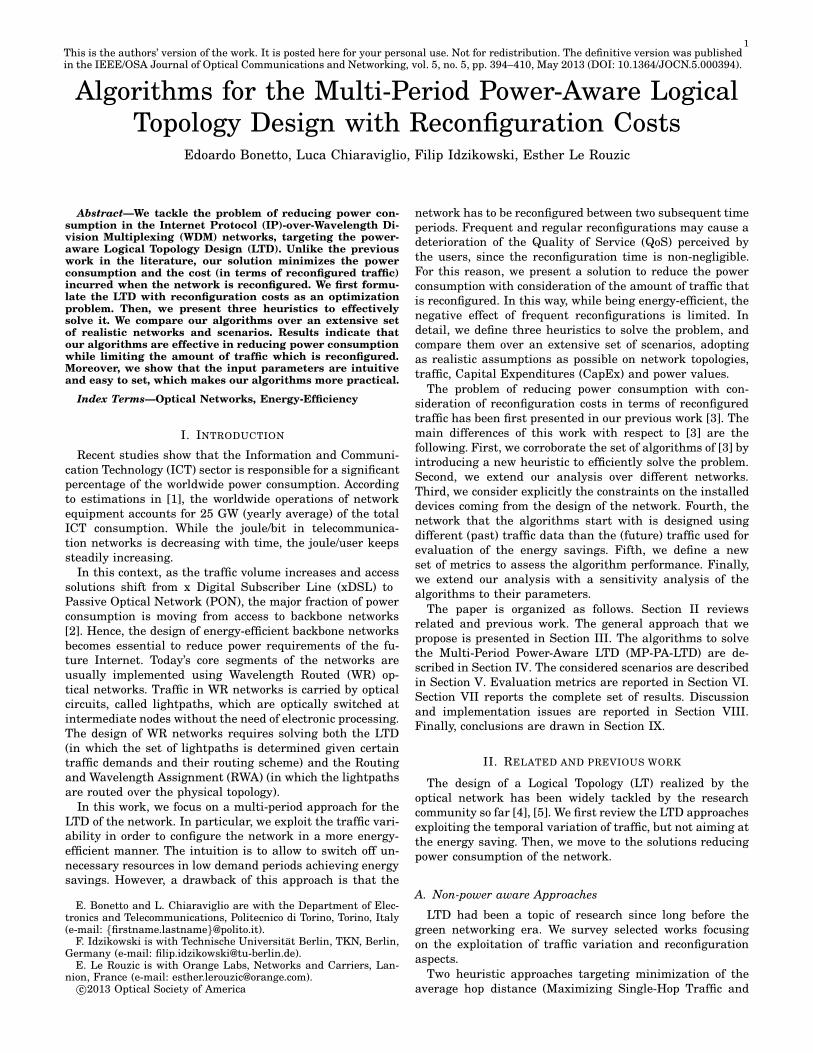
ConsumptionPowerSBN Power

Consumption ∆ t

futTpastT

MP−PA−LTD

Time

Time

TrafficTraffic

Fig. 1. Main idea of MP-PA-LTD (mind different scales of x-axes).

Architecture. The algorithm checks the fulfillment of the

QoS requirements, but the reconfiguration cost is not taken

into account. The authors of [33] perform a reality check

of Energy-Aware Routing on different network scenarios

assuming three different energy models (energy-agnostic,

idleEnergy and fully proportional). The constraints on ma-

ximum load on logical links are incorporated in the formu-

lated MILP, and analyzed in the solutions. The MILP does

not take into account reconfiguration costs. Minimization of

power consumed by router Line Cards (LCs) and chassis

in each of 12 periods over a day is investigated in [34].

The authors analyze the newly turned-on and shut down

LCs (and lightpaths), as well as the percentage of traffic

rerouted in the Virtual Topology that is produced as outcome

of the MILP solution. The reconfiguration cost is however not

included in the objective function of the formulated MILP.

A design of a complete IP-over-WDM network has been

presented in our previous work [26]. Updates of the network

configuration (including LT) for energy saving assuming

different levels of freedom of rerouting in the IP and WDM

layers are discussed. The reconfiguration cost is not included

in [26], since this work targets the assessment of the poten-

tial of energy saving in IP-over-WDM networks.

Performance of switch-off and switch-on schemes are com-

pared in [35]. The authors propose a network designed for

off-peak hour with the possibility to establish dynamic op-

tical circuits in the peak hour. Then, routing parameters are

introduced to trade between energy consumption and route

changes. Solutions of the formulated MILPs are presented,

without investigating practical heuristics.

Distributed algorithms are proposed in [36] (GRiDA), [37]

(utilization of periodic Link State Advertisements (LSAs)

describing configuration and load of links, and broadcasting

critical states) and in [38] (Distributed and Adaptive Inter-

face Switch off for Internet Energy Saving (DAISIES)). The

reconfiguration cost in terms of rerouted traffic is considered

in none of these works, while the number of reconfigurations

per node is analyzed in [36], [37].

All the works presented above are focused on the reduction

of power consumption assuming a temporal variation of

traffic, without directly targeting the reduction of the recon-

figuration costs. To solve these issues, in this work we tackle

explicitly the minimization of the weighted sum of power

consumption and reconfiguration costs. In particular, we

start from our works [39] and [40] to redesign our previous

algorithms by considering also the reconfiguration costs.

Moreover, we propose a new algorithm, called Energy Wa-

termark Algorithm (EWA) [41], which is fully adaptive and

makes decisions about establishing and releasing lightpaths.

In this way, we are able to compare different algorithms,

and discuss deeply the trade-off between power consump-

tion and reconfiguration costs. Additionally, we evaluate our

algorithms on as realistic scenarios as possible. Finally, we

differentiate between past and future traffic respectively

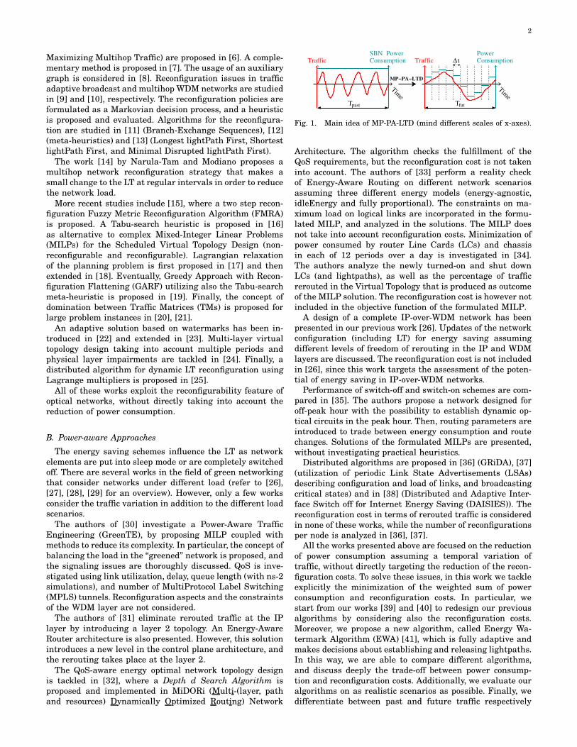
3

A B

C

DE

Fiber

OXC

Logical link

IP router

Fig. 2. Network model on exemplary logical and physical topologies.

used for the design of the Static Base Network (SBN), and

for evaluation of the energy savings achieved with heuris-

tics starting from the SBN. While the terms ‘virtual’ and

‘logical’ are used interchangeably in the related work, we

consistently use the term ‘logical’ in this work.

III. MULTI-PERIOD POWER-AWARE LOGICAL TOPOLOGY

DESIGN

In the MP-PA-LTD, we exploit the dynamic nature of

traffic, which is not constant in time, but usually follows a

day-night pattern with high traffic demands during the day

and low traffic demands during the night. Today, network

resources are allocated to constantly satisfy the maximum

demands. These resources consume energy even if not used

or underutilized. Indeed, power consumption in currently

deployed network devices is basically independent of load

[42]. Therefore, we divide the day into smaller time periods.

Each period is characterized by a TM used to design the

LT for the current period. Configuring the network for each

of these periods allows utilization of resources to a higher

extent, and consequently power can be saved by switching

off some devices. Fig. 1 reports a schematic description of

our solution. Normally, power consumption of the network

is constant, independently of the current traffic (Fig. 1 left).

With our approach, instead, the network power consumption

is wisely adapted for each time period (Fig. 1 right). However,

the network configuration (network nodes with installed

devices in active or inactive states, established lightpaths,

and routing of traffic demands) has to be changed between

two consecutive time periods. Reconfiguring means adding or

deleting lightpaths from the LT, which involves changing the

routing of the traffic over the LT. In this work we consider

the latter as a metric to quantify the reconfiguration costs.

Therefore, we define the reconfiguration cost for each light-

path as the amount of new traffic that has to be routed on

the lightpath at the beginning of the new time period. All the

notation used in this work is summarized in Appendix VIII.

A. Network and node model

We consider a backbone IP-over-WDM network schemati-

cally modeled in Fig. 2. Fibers (blue solid lines) interconnect

Optical Cross-Connects (OXCs) at the physical layer. They

are used to realize the LT at the IP layer. We model the

LT as a directed network composed of nodes and logical

links (green dashed lines). A logical link consists of all the

lightpaths established between a corresponding pair of IP

routers, independently of their realization in the physical

topology.

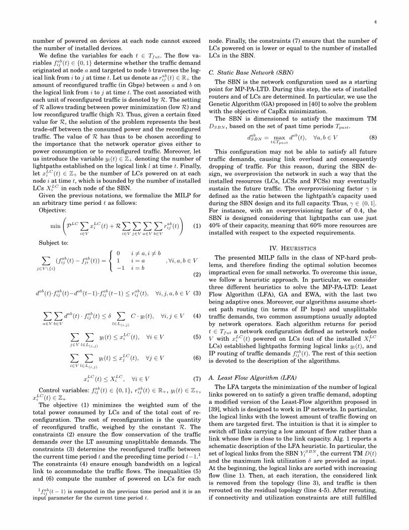
Each IP router has a modular structure, and is composed

of one or more Line Card Shelves (LCSs) interconnected by

Fabric Card Shelves (FCSs), as depicted in Fig. 3. The LCS is

the basic structure of the router. It is composed of the router

chassis, switching fabric, cooling and power supply systems.

FCS LCS

LC

LC

LC

LC

LC

LC

LCS

...

...

Fig. 3. IP router model – configuration with 2 LCSs and a FCS.

It implements the control plane and data plane software.

Furthermore, it is equipped with LCs which are responsible

for the physical connectivity of the router. Colored router

interfaces are assumed. In the case that two or more LCSs

are required, the FCSs are essential to interconnect the

LCSs. Indeed, the FCSs contain the switching fabrics that

are used for the interconnections of the LCSs. In this work,

we target reduction of the power by switching off LCs. This

choice is due to the fact that LCs are expected to have

significantly lower boot times than LCSs and FCSs, which

makes their frequent activation and deactivation possible.

We do not consider the power consumption of the OXCs

and optical amplifiers since we focus on the LTD. Moreover,

powering these devices on and off is expected to be time

consuming.

B. Mathematical model

An informal description of the problem we target is the

following. Given the current network configuration and the

set of current traffic demands, find the set of lightpaths

and corresponding LCs that must be powered on so that

the weighted sum of the power consumption and the recon-

figured traffic is minimized, subject to flow conservation

constraints, maximum lightpath utilization constraints, and

constraints on the installed devices.

More formally, let us represent the LT of an IP-over-WDM

network as a directed graph H = (V,L) where V is the set of

all nodes in the network and L is the set of supplied logical

links on which lightpaths can be established. Let L(i,j) ⊂ Ldenote the set of supplied logical links between node i and

node j. We exclude parallel logical links, therefore |L(i,j)| = 1for each (i, j) ∈ V × V .

Each logical link is formed by a trunk of parallel light-

paths. Let us define the capacity of a lightpath as C. More-

over, we denote by δ ∈ (0, 1] the maximum lightpath uti-

lization. Each lightpath needs a transmitter and a receiver

located in two LCs installed at the endpoints of the lightpath.

The power consumption of a LC is denoted as PLC .

We consider a set of time periods T consisting of past and

future time periods (T = Tpast ∪ Tfut, Tpast ∩ Tfut = ∅).

We assume to know the traffic exchanged in the past time

periods Tpast ⊂ T (Fig. 1 left) and we determine the set

of installed devices using this past traffic. We call this

procedure Static Base Network (SBN) design. At the end of

the SBN design, a set of installed devices is defined. Then

we apply the MP-PA-LTD to the SBN on future time periods

Tfut ⊂ T (Fig. 1 right). While time periods Tpast regard

the traffic before the SBN design, the future time periods

Tfut concern future traffic which we assume to be unknown

during the SBN design phase. The duration of each time

period t ∈ Tfut is denoted as ∆t. A Traffic Matrix (TM)

D(t) for each time period t ∈ T contains traffic demands

between the nodes (a, b) ∈ V × V with values dab(t). During

the MP-PA-LTD constraints of the SBN are checked – the

4

number of powered on devices at each node cannot exceed

the number of installed devices.

We define the variables for each t ∈ Tfut. The flow va-

riables fabij (t) ∈ {0, 1} determine whether the traffic demand

originated at node a and targeted to node b traverses the log-

ical link from i to j at time t. Let us denote as rabij (t) ∈ R+ the

amount of reconfigured traffic (in Gbps) between a and b on

the logical link from i to j at time t. The cost associated with

each unit of reconfigured traffic is denoted by R. The setting

of R allows trading between power minimization (low R) and

low reconfigured traffic (high R). Thus, given a certain fixed

value for R, the solution of the problem represents the best

trade-off between the consumed power and the reconfigured

traffic. The value of R has thus to be chosen according to

the importance that the network operator gives either to

power consumption or to reconfigured traffic. Moreover, let

us introduce the variable yl(t) ∈ Z+ denoting the number of

lightpaths established on the logical link l at time t. Finally,

let xLCi (t) ∈ Z+ be the number of LCs powered on at each

node i at time t, which is bounded by the number of installed

LCs XLCi in each node of the SBN.

Given the previous notations, we formalize the MILP for

an arbitrary time period t as follows:

Objective:

min

(

PLC∑

i∈V

xLCi (t) +R

∑

i∈V

∑

j∈V

∑

a∈V

∑

b∈V

rabij (t)

)

(1)

Subject to:

∑

j∈V \{i}

(fabij (t)− fab

ji (t)) =

0 i 6= a, i 6= b1 i = a−1 i = b

,∀i, a, b ∈ V

(2)

dab(t)·fabij (t)−d

ab(t−1)·fabij (t−1) ≤ rabij (t), ∀i, j, a, b ∈ V (3)

∑

a∈V

∑

b∈V

dab(t) · fabij (t) ≤ δ

∑

l∈L(i,j)

C · yl(t), ∀i, j ∈ V (4)

∑

j∈V

∑

l∈L(i,j)

yl(t) ≤ xLCi (t), ∀i ∈ V (5)

∑

i∈V

∑

l∈L(i,j)

yl(t) ≤ xLCj (t), ∀j ∈ V (6)

xLCi (t) ≤ XLC

i , ∀i ∈ V (7)

Control variables: fabij (t) ∈ {0, 1}, rabij (t) ∈ R+, yl(t) ∈ Z+,

xLCi (t) ∈ Z+

The objective (1) minimizes the weighted sum of the

total power consumed by LCs and of the total cost of re-

configuration. The cost of reconfiguration is the quantity

of reconfigured traffic, weighed by the constant R. The

constraints (2) ensure the flow conservation of the traffic

demands over the LT assuming unsplittable demands. The

constraints (3) determine the reconfigured traffic between

the current time period t and the preceding time period t−1.1

The constraints (4) ensure enough bandwidth on a logical

link to accommodate the traffic flows. The inequalities (5)

and (6) compute the number of powered on LCs for each

1fabij (t − 1) is computed in the previous time period and it is an

input parameter for the current time period t.

node. Finally, the constraints (7) ensure that the number of

LCs powered on is lower or equal to the number of installed

LCs in the SBN.

C. Static Base Network (SBN)

The SBN is the network configuration used as a starting

point for MP-PA-LTD. During this step, the sets of installed

routers and of LCs are determined. In particular, we use the

Genetic Algorithm (GA) proposed in [40] to solve the problem

with the objective of CapEx minimization.

The SBN is dimensioned to satisfy the maximum TM

DSBN , based on the set of past time periods Tpast.

dabSBN = maxt∈Tpast

dab(t), ∀a, b ∈ V (8)

This configuration may not be able to satisfy all future

traffic demands, causing link overload and consequently

dropping of traffic. For this reason, during the SBN de-

sign, we overprovision the network in such a way that the

installed resources (LCs, LCSs and FCSs) may eventually

sustain the future traffic. The overprovisioning factor γ is

defined as the ratio between the lightpath’s capacity used

during the SBN design and its full capacity. Thus, γ ∈ (0, 1].For instance, with an overprovisioning factor of 0.4, the

SBN is designed considering that lightpaths can use just

40% of their capacity, meaning that 60% more resources are

installed with respect to the expected requirements.

IV. HEURISTICS

The presented MILP falls in the class of NP-hard prob-

lems, and therefore finding the optimal solution becomes

impractical even for small networks. To overcome this issue,

we follow a heuristic approach. In particular, we consider

three different heuristics to solve the MP-PA-LTD: Least

Flow Algorithm (LFA), GA and EWA, with the last two

being adaptive ones. Moreover, our algorithms assume short-

est path routing (in terms of IP hops) and unsplittable

traffic demands, two common assumptions usually adopted

by network operators. Each algorithm returns for period

t ∈ Tfut a network configuration defined as network nodes

V with xLCi (t) powered on LCs (out of the installed XLC

i

LCs) established lightpaths forming logical links yl(t), and

IP routing of traffic demands fabij (t). The rest of this section

is devoted to the description of the algorithms.

A. Least Flow Algorithm (LFA)

The LFA targets the minimization of the number of logical

links powered on to satisfy a given traffic demand, adopting

a modified version of the Least-Flow algorithm proposed in

[39], which is designed to work in IP networks. In particular,

the logical links with the lowest amount of traffic flowing on

them are targeted first. The intuition is that it is simpler to

switch off links carrying a low amount of flow rather than a

link whose flow is close to the link capacity. Alg. 1 reports a

schematic description of the LFA heuristic. In particular, the

set of logical links from the SBN Y SBNl , the current TM D(t)

and the maximum link utilization δ are provided as input.

At the beginning, the logical links are sorted with increasing

flow (line 1). Then, at each iteration, the considered link

is removed from the topology (line 3), and traffic is then

rerouted on the residual topology (line 4-5). After rerouting,

if connectivity and utilization constraints are still fulfilled

5

Algorithm 1 Pseudo-code of LFA.

Input: Set Y SBNl from SBN, current TM D(t), maximum

utilization δOutput: Updated netConfig

1: LLs=sortLeastFlow(Y SBNl );

2: for j = 1; j ≤size(LLs); j++ do

3: disableLogicalLink(LLs[j]);4: paths=computeAllShortestPaths(D(t));5: computeAllLinkFlow(paths, D(t));6: if (checkPaths(paths) == false) ||

(checkFlows(paths, δ) == false) then

7: enableLogicalLink(LLs[j]);8: end if

9: end for

(line 6), then the selected link is definitively powered off.

Otherwise it is left on. The procedure is repeated for all the

logical links (line 2). In the case that the current TM cannot

be satisfied by the SBN, LFA does not power off any link.

B. Genetic Algorithm (GA)

The GA was first introduced in [40], where it optimizes just

the power consumption of the network. It has been adapted

to solve the MP-PA-LTD to directly minimize the power

consumption and the reconfiguration cost. The GA is a meta-

heuristic based on the principles of the natural evolution:

the initial population evolves through several generations

in which only a subset of the individuals survive from one

generation to the following one.

Each individual represents a LT. Only feasible individuals

can be part of the population. In particular, an individual

is feasible if its corresponding LT satisfies the TM and

the constraints (7) on the maximum number of powered

on devices. If the GA cannot find any feasible solution, the

constraints (7) are relaxed and dummy LCs are installed.

However, the traffic routed over these additional LCs is

considered as overload.

The individuals survive through generations depending on

their fitness value which is defined as the weighted sum of

normalized power consumption and normalized reconfigu-

ration cost. Thus, the GA optimizes the same objective (1)

as the mathematical model presented in Section III-B. The

normalization of the power and of the reconfiguration cost is

performed with respect to the possible worst case, i.e., every

node has to process all the traffic of the current TM. The

sum is weighted by the parameter α ∈ [0, 1], which is used,

similarly to the constant R of (1), to trade between power

and reconfiguration costs.

Alg. 2 describes briefly how the GA works. The algorithm

requires as input the network configuration from previous

time period t − 1 and the current TM D(t). Moreover, three

algorithm parameters have to be provided: the maximum

number of generations without improvements M , the pop-

ulation size S and the offspring size K. At the beginning,

the first population is randomly generated (line 1). After

this step the fitness is evaluated (line 3) and the evolution

process begins (line 4). At each generation, the reproduction

and the selection phases are repeated. In particular, new

individuals are created during the reproduction phase (line

5), starting from some other individuals that have been

chosen as parents. Then, a new population is created (line

Algorithm 2 Pseudo-code of GA.

Input: netConfig from period t− 1, current TM D(t), α, M ,

S, KOutput: Updated netConfig

1: population=generateFirstPopulation(D(t), netConfig, S,

α);

2: i=0;

3: fitness=evaluateFitness(population, α);

4: while (i ≤ M ) do

5: offspring=generateOffspring(population, D(t), netCon-

fig, α, K);

6: population=selectPopulation(population, offspring, α,

S);

7: newFitness=evaluateFitness(population, α);

8: if (newFitness ≥ fitness) then

9: i++;

10: else

11: i=0;

12: fitness=newFitness;

13: end if

14: end while

15: netConfig=applyConfiguration(population);

6) by selecting the individuals with best fitness value from

the old population and its offspring. At each generation, the

best fitness value among all the individuals is selected and

stored (line 7). If the fitness has not improved with respect to

the previous generation, the current number of generations

without improvement is incremented (line 9). The evolution

process stops when the fitness value has not improved for

more than a maximum number of generations (line 4). At

the end, the individual with the best fitness is chosen, and

the set of powered on lightpaths is updated (line 15).

C. Energy Watermark Algorithm (EWA)

The EWA is an adaptive algorithm based on [22] which

uses a low and a high watermark (WL and WH) in order

to switch off as many LCs as possible without exceeding

maximum utilization of last lightpath on a logical link ψ.

Each watermark is defined as a threshold on the utilization

of the last lightpath on a logical link. In particular, WH

triggers attempts to establish additional lightpath(s) in order

to avoid overload of the network and ensure appropriate QoS.

On the contrary, WL triggers attempts to release lightpath(s)

in order to save energy.

The algorithm takes as input the network configuration in

previous time period t− 1 TM D(t) for the current period t,capacity of a lightpath (WDM channel) C, WL, WH and ψ.

Alg. 3 shows the main pseudocode of EWA. The complete

algorithm description is reported in [41]. EWA first checks

whether all the demands in the current network configura-

tion are routable, and iteratively tries to establish additional

lightpaths for the unroutable demands (if any), starting

from the largest ones (line 1). The logical links on which

watermarks are exceeded are identified next (line 2), and

violation of the WH is checked, starting from the logical links

with the highest utilization of the last lightpath (line 3). For

each overloaded logical link (from the most overloaded to

the least overloaded), the algorithm first tries to increase the

capacity of the logical link if a demand with the same source

and target nodes flows through it. If this is not the case,

6

Algorithm 3 Pseudo-code of EWA.

Input: netConfig from period t−1, current TM D(t), C, WL,

WH , ψOutput: Updated netConfig

1: ensureDemandsRoutability(netConfig, D(t), C);

2: sortedLLsExceedingWMs = getSortedLLsExceeding-

WMs(netConfig, D(t), WL, WH);

3: establishNecessaryLpaths(netConfig, D(t), C, sortedLL-

sExceedingWMs, WL, WH);

4: releaseUnnecessaryLpaths(netConfig, D(t), sortedLL-

sExceedingWMs, WL, WH , ψ);

attempts are made to establish lightpath(s) for the possibly

biggest demand flowing over the overloaded logical link.

Once the load is lower than WH for all logical links, or it is

impossible to reduce overload anymore, violation of the WL

is checked starting from the least loaded logical links (line

4). One lightpath at a time is tried to be released, making

sure that ψ is not exceeded.

Differently from [22], EWA is able to add or delete more

than one lightpath during the execution of the algorithm

(lines 1, 3 and 4). Moreover, EWA considers the case in

which adding some lightpath(s) does not forbid deleting other

lightpath(s). Finally, parameter ψ is added in order to trade

between QoS and energy saving. These differences result in

a different approach in establishing and releasing lightpaths

compared to [22].

V. SCENARIOS

We first describe the considered networks and the traffic

assumptions. Next, we detail the CapEx and power consump-

tion figures of the adopted network components.

A. Networks and Traffic

We consider traffic demands that have been measured in

three different networks: Abilene (12 nodes), Germany17 (17

nodes) and Geant (22 nodes). The physical supply networks

and the corresponding TMs are available in [26], [43]. More-

over, each lightpath has capacity C equal to 40 Gbps.

TMs with granularity ∆t equal to 15 minutes are avail-

able for Geant, while for Abilene and Germany17 TMs are

measured every 5 minutes. In order to be consistent, we

compute TMs with granularity 15 minutes for Abilene and

Germany17 by taking the maximum values out of the 3

corresponding 5-minute TMs.

Total period covered by Tpast (design of the SBN) equals 1

month for Abilene and Geant. Note that fine granular TMs

(5 min.) cover only one day in the Germany17 network [43].

Therefore we use 12 TMs with time granularity equal to 1

month over the year 2004 to dimension the SBN. Since these

TMs contain average values of traffic demands over a month,

they alter temporal peaks of the traffic, and hence higher

overprovisioning is needed during the design of the SBN.

We consider the total period covered by Tfut equal to 1

day. We select the evaluation days belonging to two different

types (Working Day (WD) and WeekEnd day (WE)) in order

to compare the MP-PA-LTD algorithms under various traffic

conditions.

The original TMs from [43] are scaled in order to mimic

actual traffic demands and to have comparable load in the

three networks. We introduce the total demand per node

d|V | =∑

(a,b)∈V ×VdabSBN/|V |, and the corresponding unit Gi-

gabit per second per node (Gpn). We consider three different

load assumptions, and scale DSBN to have the total demand

per node equal to 100, 300 and 500 Gpn. The same scaling

factors as for DSBN are used for D(t) for each t ∈ Tfut.

The networks, as well as the traffic data that we used

for both the design of the SBN and evaluation of energy

savings are summarized in Table I. Total demand (defined

as∑

(a,b)∈V ×Vdab(t)) over time is indicated (as TRF) in

Figures 4(a) and 5(a) for two exemplary days (2004-08-27

for Abilene and 2005-06-11 for Geant). We do not present

all traffic patterns due to lack of space. More details can be

found in [41].

B. Power and CapEx Data

Cisco CRS-1 router [44] was used to parameterize our

study. Each LCS can accommodate up to WLCS = 16 LCs,

and a FCS can interconnect up to WFCS = 9 LCSs. The power

consumption values have been taken from [45]. In detail, a

LCS consumes PLCS = 2920 W and a FCS consumes PFCS

= 9100 W. We consider as LC the “Cisco CRS 4-port 10-GE

Tunable WDMPHY Interface Module” with the “Cisco CRS-1

Modular Services Card”, consuming together PLC = 500 W.

The CapEx values used during the design of the SBN have

been taken from [46]. In particular, we adopt values of 13.37,

16.67 and 53.35 units to LC, LCS and FCS, respectively.

VI. METRICS

We describe the metrics adopted to assess the algorithms

performance. We first introduce the power consumption of

all active LCs in the network:

PLC(t) = PLC∑

i∈V

xLCi (t) (9)

The energy consumption due to LCs is then defined as:

ELC =∑

t∈Tfut

PLC(t)∆t (10)

Moreover, we account also for the power of LCSs and FCSs.

The number of LCSs used at each node is expressed as:

xLCSi (t) = ⌈xLC

i (t)/WLCS⌉ (11)

Similarly, one FCS is used to interconnect up to WFCS LCSs:

xFCSi (t) =

{

0 if xLCSi (t) ≤ 1

⌈xLCSi (t)/WFCS⌉ otherwise

(12)

We define the power consumption of active LCSs in the

network as:

PLCS(t) = PLCS∑

i∈V

xLCSi (t) (13)

Similarly, the power consumption of active FCSs is defined

as:

PFCS(t) = PFCS∑

i∈V

xFCSi (t) (14)

The total network energy consumption is hence defined as:

ETOT =∑

t∈Tfut

[

PLC(t) + PLCS(t) + PFCS(t)]

∆t (15)

Together with energy consumption, we are also interested

in assessing the performance of our algorithms in terms of

7

TABLE ICONSIDERED NETWORKS AND TRAFFIC DATA [43]

Network Nodes Phy. supply links (bidir.) TMs considered at SBN design (Tpast) TMs to evaluate energy savings (Tfut)

Abilene 12 15 max. between 2004-07-01 and 2004-07-31(granularity of 5 min.)

every 15 min. over 2004-08-27 (WD), 2004-08-28(WE), 2004-08-29 (WE), 2004-09-02 (WD)

Geant 22 36 max. between 2005-05-05 and 2005-06-04(granularity of 15 min.)

every 15 min. over 2005-06-07 (WD), 2005-06-10(WD), 2005-06-11 (WE), 2005-06-12 (WE)

Germany17 17 26 max. between 2004-01 and 2004-12(granularity of 1 month)

every 15 min. over 2005-02-15 (WD)

reconfigured traffic. We therefore introduce the reconfigura-

tion ratio2 over all subsequent pairs of time periods in Tfut

as:

ξ =

∑

t∈Tfut

∑

i∈V

∑

j∈V

∑

a∈V

∑

b∈Vrabij (t)

∑

t∈Tfut

∑

a∈V

∑

b∈Vdab(t)

(16)

This metric captures the amount of traffic that is reconfig-

ured over all time periods in Tfut, normalized by the total

amount of traffic that is exchanged in the network. Note that

the reconfigured traffic may be counted multiple times (as

many times as many logical links a traffic demand passes

from its source to its target), so ξ may be greater than 1.

Finally, we define the overload ratio metric φ to capture

overload traffic in all periods t ∈ Tfut:

φ =

∑

t∈Tfut

∑

i∈V

∑

j∈Vχij(t)

∑

t∈Tfut

∑

a∈V

∑

b∈Vdab(t)

(17)

where χij(t) is defined for each t ∈ Tfut, i ∈ V and j ∈ V as:

χij(t) = max

∑

a∈V,b∈V

dab(t) · fabij (t)−

∑

l∈L(i,j)

Cyl(t), 0

(18)

φ should be as low as possible (ideally 0) to prevent service

disruptions and deterioration of QoS. Note that we account

as overload each hop between a source and a target, even

though the traffic may get dropped already at the first hop.

Therefore, also φ may be greater than 1.

VII. RESULTS

We have implemented the algorithms presented in Sec-

tion IV on custom simulators written in C++ and Java.

The LFA and GA simulations are run on a server machine

equipped with 2 Quad CPU at 2.66 GHz and 4 GB of RAM.

The EWA simulations are run on a personal computer with a

Dual Core CPU at 2.4 GHz and 2 GB of RAM. In particular,

we start considering SBN with d|V | = 300 Gpn of traffic

and overprovisioning γ = 0.5. Unless specified otherwise,

we adopt the following set of algorithm parameters: δ = 1.0for LFA, α = 0.1, M = 500, S = 30 and K = 20 for GA,

WL = 0.1, WH = 0.9 and ψ = WH for EWA. We first

compare the algorithms with the following metrics: LCs daily

energy consumption ELC , total daily energy consumption

ETOT , reconfiguration ratio ξ, and overload ratio φ. Table II

reports ELC for the different scenarios, considering working

and weekend days (WE label in the table). Focusing on the

Abilene case, ELC is lower for weekend days than working

days since traffic is lower and hence more LCs are powered

off. For example, considering the GA, ELC is 821.75 kWh

on 2004-09-02, and 689.5 kWh on 2004-08-29. Then, ELC is

2Note that rabij (t) and ξ take no value in the first period of Tfut.

higher for LFA: this is due to the fact that LFA switches off

entire logical links rather than single lightpaths. However,

turning off a logical link requires rerouting of the entire

amount of traffic flowing on it, which is not always possible.

This in turn leads to an increase of energy consumption, with

ELC always higher than 1645 kWh. On the contrary, both

EWA and GA guarantee lower energy consumption, since

they work on single lightpaths rather than logical links.

We then extend our analysis to the Germany17 and Geant

networks. In particular, all the heuristics consume a larger

amount of energy in Germany17 network than in Abilene.

This is quite intuitive, since Germany17 has more nodes

than Abilene. However, despite the Geant network being

bigger than Germany17, the energy consumption on at least

three out of four considered days in the Geant network

is lower than in Germany17 on 2005-02-15. This can be

explained by the traffic patterns on the days considered for

evaluation of the heuristics, and by the overprovisioning of

the SBNs. The overprovisioning of the Germany17 SBN is

different from the overprovisioning of the other two networks

despite using the same parameter γ. This is caused by

the fact that the traffic data available for the Germany17

network contains only one day of TMs with fine granularity

(see Section V-A and [43]). Therefore the TMs of granularity

of one month were used to design the SBN (see Table I).

Since the values in the TMs are average values over the

considered period duration, the traffic peaks are averaged

out, and are not included in DSBN , which is calculated

by taking maximum values for each demand over all TMs

(see Eq. (8)). Interestingly, EWA and GA consume similar

amount of energy in the Germany17 network compared to

LFA suggesting that, for this network, it is difficult to turn

off single lightpaths. This is caused by the fact that traffic

in the Germany17 network is centralized in Frankfurt [26].

Only 9 out of 97 logical links not attached to Frankfurt in

the SBN are composed of more than one lightpath. The LFA

tries to switch off each logical link, however, since most of

the links are composed of just a single lightpath, there is

little difference to EWA and GA, which try to switch off

single lightpaths, and not logical links. The (relatively little)

advantage in terms of energy consumption that EWA and

GA have over LFA in the Germany17 network is caused

by the logical links attached to Frankfurt (21 out of 26 are

composed of more than one lightpath), and the possibility of

establishing logical links not existing in the SBN. Finally, we

point out that EWA guarantees lower energy consumption

ELC with respect to GA and LFA in the Geant network

(Table II).

In the following, we compare the heuristics considering

the total energy consumption ETOT . Table III reports the

main results. In particular, ETOT is higher than ELC , since

we are accounting also for the power of LCSs and FCSs.

8

TABLE IILINE CARD DAILY ENERGY CONSUMPTION ELC [KWH]

Scenario LFA EWA GA

2004-08-27 Abilene 2205.37 693.37 771.25

2004-08-28 Abilene (WE) 1673 587.75 697.875

2004-08-29 Abilene (WE) 1645.37 607.50 689.5

2004-09-02 Abilene 2255.62 712.75 821.75

2005-02-15 Germany17 2378.75 1946 1739

2005-06-07 Geant 3625.75 1312 1510.38

2005-06-10 Geant 2077 1231 1312.5

2005-06-11 Geant (WE) 2206.37 1136.12 1244.13

2005-06-12 Geant (WE) 2004.12 1061.5 1209.13

TABLE IIITOTAL DAILY ENERGY CONSUMPTION ETOT [KWH]

Scenario LFA EWA GA

2004-08-27 Abilene 4246.25 1534.33 1612.21

2004-08-28 Abilene (WE) 3385.65 1428.71 1538.84

2004-08-29 Abilene (WE) 3338.97 1448.46 1530.46

2004-09-02 Abilene 4330.29 1589.77 1683.75

2005-02-15 Germany17 5467.78 4729.9 4302.93

2005-06-07 Geant 7753.17 3391.11 3632.37

2005-06-10 Geant 4847.14 3246.36 3266.59

2005-06-11 Geant (WE) 5081.82 2997.75 3107.17

2005-06-12 Geant (WE) 4685.66 3024.23 3046.11

However, both GA and EWA are able to reduce the total

energy consumption with respect to LFA, especially during

weekends. These results confirm our intuition that minimi-

zing the power consumption of LCs is of great benefit also

for reducing the total power consumption of the network,

assuming the possibility to switch off and on the LCSs and

FCSs installed in the SBN.

As the next step, we compare the heuristics in terms

of the reconfiguration ratio ξ. Table IV reports the results

for the different scenarios. Intuitively, a ratio ξ approach-

ing 1 indicates that the amount of reconfigured traffic is

comparable with the total amount of traffic demands. This

condition is not of benefit in a network, since it might have

a negative impact on the QoS of users due to temporary

service disruptions and network congestion as many devices

are changing their operational state. Focusing on the Abilene

network, ξ is typically larger than 0.66 for LFA. On the

contrary, ξ is clearly reduced by the other heuristics, being

lower than 0.15 and 0.18 for EWA and GA, respectively. This

means that targeting explicitly the reconfiguration cost has

a positive feedback on ξ. Similar considerations hold for the

Germany17 and Geant networks. Finally, observe also that

ξ does not significantly change over the different days, i.e.,

between working days and weekend days. This is due to the

fact that a larger amount of traffic exchanged in the network

(denominator of Eq. (16)) implies also a larger amount of

reconfigured traffic (numerator of Eq. (16)).

Finally, Table V reports the overload ratio over the diffe-

rent scenarios. Intuitively, φ should be kept as low as possible

to limit the negative effects of packet dropping. Focusing

on the Abilene network, φ = 0 for both EWA and GA. On

the contrary, φ > 0 for different days when LFA is adopted.

This is due to the intrinsic behavior of the algorithm: since

LFA starts from SBN and tries to switch off logical links,

in some cases the set of logical links provided by the SBN

TABLE IVRECONFIGURATION RATIO ξ

Scenario LFA EWA GA

2004-08-27 Abilene 0.75 0.13 0.16

2004-08-28 Abilene (WE) 0.72 0.15 0.18

2004-08-29 Abilene (WE) 0.70 0.15 0.17

2004-09-02 Abilene 0.66 0.12 0.14

2005-02-15 Germany17 0.35 0.1 0.12

2005-06-07 Geant 0.40 0.09 0.11

2005-06-10 Geant 0.49 0.08 0.12

2005-06-11 Geant (WE) 0.48 0.1 0.13

2005-06-12 Geant (WE) 0.44 0.08 0.11

TABLE VOVERLOAD RATIO φ

Scenario LFA EWA GA

2004-08-27 Abilene 7 × 10−5 0 0

2004-08-28 Abilene (WE) 0 0 0

2004-08-29 Abilene (WE) 3 × 10−5 0 0

2004-09-02 Abilene 2 × 10−3 0 0

2005-02-15 Germany17 5 × 10−3

2 × 10−2

4 × 10−6

2005-06-07 Geant 8 × 10−4 0 0

2005-06-10 Geant 0 0 0

2005-06-11 Geant (WE) 7 × 10−4 0 0

2005-06-12 Geant (WE) 3 × 10−5

3 × 10−5 0

is not sufficient to satisfy the peak traffic.3 Consequently,

the overload is larger than zero, even if it is kept quite low,

i.e., typically lower than 10−3. On the contrary, both EWA

and GA can accommodate the traffic demands more wisely,

since they integrate the possibility to add lightpaths while

satisfying the constraint of installed LCs in each network

node. Table V reports also the results for the Germany17

network. In this case, φ > 0 for all the heuristics, suggesting

that the SBN is not sufficient to satisfy the traffic without

exceeding the number of installed LCs. This is due to the

fact that the SBN is designed with dabSBN calculated using

monthly averages of demand values (see Section V). Finally,

the Table V reports the results for the Geant network. In

this case, φ < 8× 10−4 and φ < 3× 10−5 for LFA and EWA,

respectively. However, the overload is limited, since it occurs

only in the first 15-minute period on 2005-06-12, and can

be avoided by using the network configuration from the last

period of 2005-06-11 instead of the SBN as a starting point.

GA avoids overload for all the periods in the Geant network.

A. Time Variation

We then investigate the temporal behavior of the algo-

rithms. In particular, we start considering the Abilene net-

work4 and the day 2004-08-27. Fig. 4(a) shows the power

consumption of LCs versus time PLC(t). Power follows a day-

night trend of traffic (right y-axis) for GA and EWA. Higher

power is consumed by LFA, whose trend presents also spikes.

In some cases LFA finds an aggressive configuration with

many logical links switched off. Hence, the total power

consumption is close to the other heuristics. However, the

aggressive configuration is not able to accommodate traffic

3Recall that we have adopted different time periods for designingthe SBN and for evaluating the heuristics.

4We do not change the time zone of the original TMs [43], thereforethe day-night patterns in Abilene look shifted in time.

9

0

20

40

60

80

100

120

140

00:00 06:00 12:00 18:00 00:00 0

1

2

3

4

5

6

7

PL

C[k

W]

To

tal

dem

and

[T

bp

s]

Time

LFAEWA

GATRF

(a) Power consumption and total demand

0

100

200

300

400

500

600

700

800

00:00 06:00 12:00 18:00 00:00

To

tal

reco

nfi

gu

red

tra

ffic

[G

bp

s]

Time

LFAEWA

GA

(b) Total reconfigured traffic

Fig. 4. Power consumption of active Line Cards, total demand andtotal reconfigured traffic in the Abilene network.

for a long period, i.e., more than one TM. This in turn leads

to a new, less aggressive configuration of logical links with

consistently higher power consumption. On the contrary,

observe how GA and EWA are able to reduce power, with

smooth power transitions. Note that the power consumption

of all LCs installed in the SBN is more than 142 kW (not

reported in the figure), thus we can conclude that our heuris-

tics are effective in reducing the power consumption. To give

more insight, Fig. 4(b) reports the total reconfigured traffic

(sum of rabij (t) in (1)), expressed in Gbps. Both GA and EWA

reduce the amount of traffic that is reconfigured, so that the

reconfigured traffic is always smaller than 220 Gbps. On the

contrary, LFA always requires higher amount of reconfigured

traffic.

We then extend our analysis considering the Geant net-

work and the 2005-06-10 day. Fig. 5(a) reports power con-

sumption of LCs versus time PLC(t). In this case, the power

consumption of the always on network (SBN) is 276 kW,

while our heuristics guarantee that power consumption is al-

ways lower than 105 kW. Again, a day-night behavior clearly

emerges. Finally, the total reconfigured traffic is reported in

Fig. 5(b). In this case, lower reconfigurations occur during

the night for the three algorithms, suggesting that during

the night the set of powered on devices does not frequently

vary.

B. Impact of Static Base Network (SBN)

In this section, we investigate the impact of the SBN

design on the performance of our heuristics. In particular,

we vary the overprovisioning factor γ in the range [0.2-

0.5], trading between large and medium overprovisioning

of SBNs. Intuitively, large overprovisioning requires more

0

20

40

60

80

100

120

00:00 06:00 12:00 18:00 00:00 0

1

2

3

4

5

6

PL

C [

kW

]

To

tal

dem

and

[T

bp

s]

Time

LFAEWA

GATRF

(a) Power consumption and total demand

0

500

1000

1500

2000

2500

00:00 06:00 12:00 18:00 00:00

To

tal

reco

nfi

gu

red

tra

ffic

[G

bp

s]

Time

LFAEWA

GA

(b) Total reconfigured traffic

Fig. 5. Power consumption of active Line Cards, total demand andtotal reconfigured traffic in the Geant network.

capacity to be installed, implying more power consumption

but also more freedom in choosing which devices to power off.

We assume traffic per node d|V | equal to 300 Gpn, and focus

on the days 2004-08-27 for Abilene, 2005-06-10 for Geant

and 2005-02-15 for Germany17.

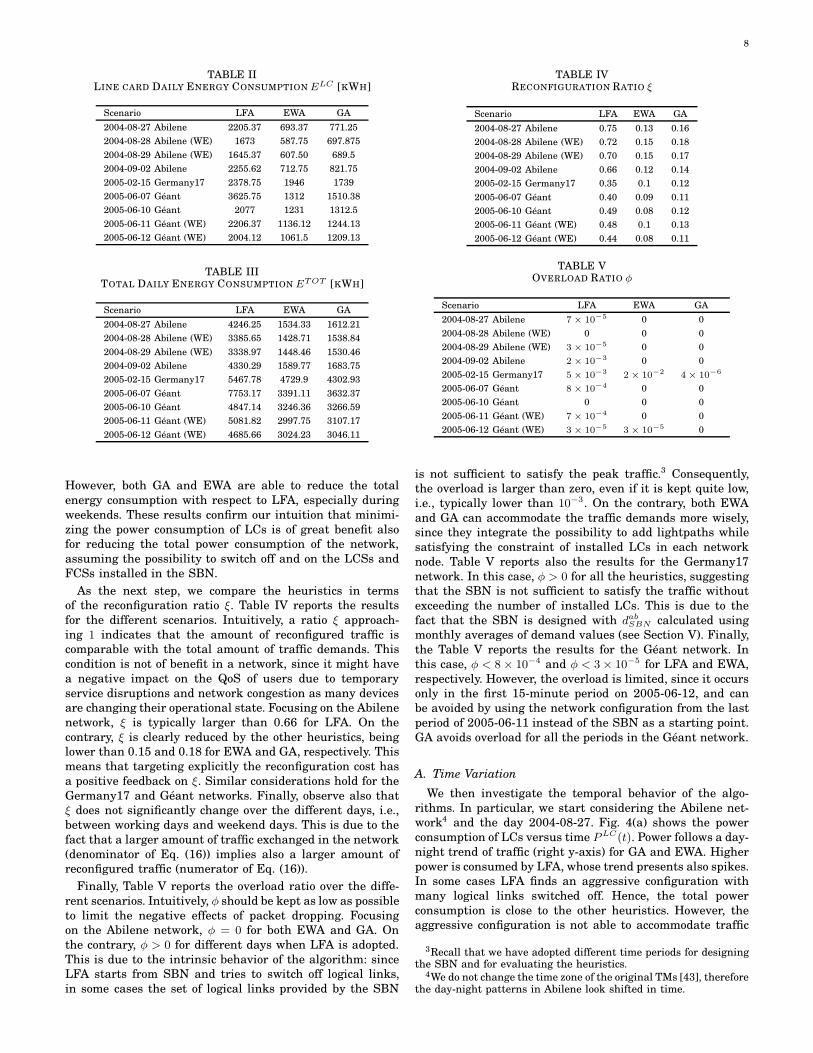
Fig. 6 reports ELC and ξ for the different scenarios. γ im-

pacts the performance of LFA. In particular, for the Abilene

scenario ELC of LFA passes from 2200 kWh with γ = 0.5 to

more than 4500 kWh with γ = 0.2. The reason why energy

consumed by LCs in a network using LFA increases with

increasing overprovisioning of the SBN is that the logical

links that LFA did not switch off are still overprovisioned

proportionally to the overprovisioning of the SBN. On the

contrary, when considering the reconfiguration ratio ξ, the

variation of SBN does not impact consistently the results.

Moreover, when considering the Germany17 network, all the

algorithms consume a similar amount of energy for γ = 0.5and γ = 0.3. This is due to the fact that, for this type of

network, it is more difficult to turn off LCs due to different

behavior of traffic used to design the SBN. Differently from

LFA, both EWA and GA present just minor oscillations of

energy consumption and reconfiguration ratio for all the

values of γ. This is due to the fact that both algorithms are

not restricted to logical links existing in the SBN, and that

they consider establishment and release of single lightpaths,

and not whole logical links.

C. Impact of Load Variation

Keeping the day-night traffic variation, we vary the total

traffic per node d|V | between 100 Gpn and 500 Gpn in the

SBN design phase with γ set to 0.5. We consider the day

2004-08-27 for Abilene, and the day 2005-06-10 for Geant.

10

0

500

1000

1500

2000

2500

3000

3500

4000

4500

5000

0.2 0.3 0.4 0.5

EL

C [

kW

h/d

ay]

Overprovisioning factor γ

LFAEWA

GA

(a) ELC for Abilene

0

500

1000

1500

2000

2500

3000

3500

4000

4500

5000

0.2 0.3 0.4 0.5

EL

C [

kW

h/d

ay]

Overprovisioning factor γ

LFAEWA

GA

(b) ELC for Geant

0

500

1000

1500

2000

2500

3000

3500

4000

0.2 0.3 0.4 0.5

EL

C [

kW

h/d

ay]

Overprovisioning factor γ

LFAEWA

GA

(c) ELC for Germany17

0

0.2

0.4

0.6

0.8

1

0.2 0.3 0.4 0.5

Rec

onfi

gura

tion R

atio

ξ

Overprovisioning factor γ

LFAEWA

GA

(d) ξ for Abilene

0

0.2

0.4

0.6

0.8

1

0.2 0.3 0.4 0.5

Rec

onfi

gura

tion R

atio

ξ

Overprovisioning factor γ

LFAEWA

GA

(e) ξ for Geant

0

0.2

0.4

0.6

0.8

1

0.2 0.3 0.4 0.5

Rec

onfi

gura

tion R

atio

ξ

Overprovisioning factor γ

LFAEWA

GA

(f) ξ for Germany17

Fig. 6. SBN Variation: Energy consumption and reconfiguration ratio in the Abilene and Geant networks.

0

500

1000

1500

2000

2500

3000

3500

4000

100 Gpn 300 Gpn 500 Gpn

EL

C [

kW

h/d

ay]

Traffic Per Node d|V|

LFAEWA

GA

(a) Energy Consumption

0

0.2

0.4

0.6

0.8

1

100 Gpn 300 Gpn 500 Gpn

Rec

on

fig

ura

tio

n r

atio

ξ

Traffic Per Node d|V|

LFAEWA

GA

(b) Reconfiguration Ratio

Fig. 7. Load Variation: Energy consumption and reconfigurationratio in the Abilene network.

0

500

1000

1500

2000

2500

3000

3500

100 Gpn 300 Gpn 500 Gpn

EL

C [

kW

h/d

ay]

Traffic Per Node d|V|

LFAEWA

GA

(a) Energy Consumption

0

0.2

0.4

0.6

0.8

1

100 Gpn 300 Gpn 500 Gpn

Rec

on

fig

ura

tio

n r

atio

ξ

Traffic Per Node d|V|

LFAEWA

GA

(b) Reconfiguration Ratio

Fig. 8. Load Variation: Energy consumption and reconfigurationratio in the Geant network.

Fig. 7 reports the results for the Abilene network. ELC is

increasing with d|V | for all the algorithms (as expected).

Interestingly, all the algorithms consume a similar amount

of energy for d|V | = 100 Gpn, since under little load a

minimum number of LCs has to be always powered on to

guarantee connectivity. However, as traffic increases, the

LFA consumes more energy than GA and EWA. Moreover,

ξ decreases as d|V | increases for EWA and GA, suggesting

that these algorithms can wisely accommodate the increase

of traffic by limiting the amount of reconfigurations.

Similar considerations hold also for the Geant network,

reported in Fig. 8. It is interesting to note that the GA

consumes slightly more energy than LFA under low load

(d|V | = 100 Gpn).

D. Sensitivity Analysis

In this section we evaluate the impact of the algorithm

parameters on ELC and ξ. We adopt the following scenarios:

the day 2004-08-27 for Abilene, and the day 2005-06-10 for

Geant. We set γ = 0.5 and d|V | = 300 Gpn.

We first consider the LFA algorithm over the Abilene

scenario. In particular, we vary the maximum logical link

utilization δ. Fig. 9(a) reports ELC and ξ for δ = [0.5, 1.0].The energy consumption decreases as δ increases. This is

due to the fact that, as δ approaches 1, it is easier to

shift traffic to unused logical links and consequently save

energy. However, this is not beneficial for the reconfiguration

ratio, with ξ passing from 0.37 with δ = 0.5 to 0.75 with

δ = 1.0, suggesting that the algorithm is too aggressive in

selecting the set of devices to be powered off. Fig. 9(b) reports

the results for the Geant network. Also here the energy is

minimized for δ = 1.0, while ξ ranges between 0.45 and 0.52.

We then consider the EWA algorithm. We vary both the

low threshold WL and the high threshold WH . ELC and

ξ for the Abilene network are reported in Fig. 10(a) and

Fig. 10(b), respectively. Interestingly, the energy consump-

tion steadily increases for WL ≤ 0.3 and WH ≤ 0.3, while

the reconfiguration ratio is minimized. This is due to the

fact that with this setting the algorithm tries to switch off

lightpaths (low WL) less frequently, but many devices are

required to be powered on (overprovisioning due to low WH).

Conversely, with increasing values of watermarks (WL > 0.3and WH > 0.4) the energy consumption decreases, but the

reconfiguration ratio increases. Intuitively, for high values of

WL the algorithm is more aggressive in switching off devices,

while for high WH the algorithm tends to save more power

since lightpath utilization increases. However, a good trade-

off is guaranteed by setting WL = 0.1 and WH > 0.4. Fig. 11

reports the results for the Geant network. Also here the

energy is clearly minimized for high values of WL and WH

(conversely for the reconfiguration ratio). A good trade-off in

this case is to set WL = 0.1 and WH = 0.9.

Finally, we have performed a sensitivity analysis on the

GA algorithm. In particular, we have varied α, which weighs

differently the reconfiguration costs with respect to power

consumption. Similarly to R introduced in Section III-B, the

parameter α allows to trade between the power consumption

and the reconfigured traffic when searching for the optimal

solution. Thus, α should be set according to the importance

given to the two metrics. Fig. 12(a) reports ELC and ξ for

the Abilene scenario. Astonishingly, ξ passes from more than

0.9 with α = 0.9 to less than 0.14 with α = 0.1, suggesting

that the reconfiguration cost steadily increases when power

consumption becomes the predominant term in the utility

11

0

500

1000

1500

2000

2500

3000

3500

0.5 0.6 0.7 0.8 0.9 1.0 0

0.125

0.25

0.375

0.5

0.625

0.75

0.875

EL

C [

kW

h/d

ay]

Rec

onfi

gura

tion r

atio

ξ

Maximum lightpath utilization δ

Energy ConsumptionReconfiguration Ratio

(a) Abilene

0

500

1000

1500

2000

2500

3000

0.5 0.6 0.7 0.8 0.9 1.0 0

0.1

0.2

0.3

0.4

0.5

0.6

EL

C [

kW

h/d

ay]

Rec

onfi

gura

tion r

atio

ξ

Maximum lightpath utilization δ

Energy ConsumptionReconfiguration Ratio

(b) Geant

Fig. 9. LFA Sensitivity Analysis for the Abilene and Geant networks.

0.10.2

0.30.4

0.50.6

0.70.8

0.90.1

0.20.3

0.40.5

0

1000

2000

3000

WHW

L

EL

C [kW

h/d

ay]

0

500

1000

1500

2000

2500

3000

(a) Energy Consumption

0.10.2

0.30.4

0.50.6

0.70.8

0.9

0.10.2

0.30.4

0.5

0

0.05

0.1

0.15

0.2

WHW

L

Re

co

nfig

ura

tio

n R

atio

ξ

0

0.02

0.04

0.06

0.08

0.1

0.12

0.14

0.16

0.18

(b) Reconfiguration Ratio

Fig. 10. EWA Sensitivity Analysis for the Abilene network.

0.10.2

0.30.4

0.50.6

0.70.8

0.9

0.10.2

0.30.4

0.5

0

500

1000

1500

2000

WHW

L

EL

C [kW

h/d

ay]

0

200

400

600

800

1000

1200

1400

1600

1800

(a) Energy Consumption

0.10.2

0.30.4

0.50.6

0.70.8

0.90.1

0.20.3

0.40.5

0

0.05

0.1

0.15

WHW

L

Re

co

nfig

ura

tio

n R

atio

ξ

0

0.02

0.04

0.06

0.08

0.1

(b) Reconfiguration Ratio

Fig. 11. EWA Sensitivity Analysis for the Geant network.

function. On the other hand, ELC increases as α decreases

and reaches an asymptote of about 540 kWh/day. To give

more insight, we have performed the sensitivity analysis also

for the Geant network, reported in Fig. 12(b). Again, observe

how much the choice of α is critical to trade between the

reconfiguration costs and energy consumption. The obtained

results suggest then that it may be better to choose a low

value for α, since, in that case, the reconfigured traffic is

effectively minimized, while the power consumption of the

network is not affected too much.

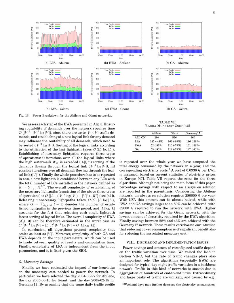
E. Power Breakdown

We then investigate how much energy is consumed by com-

ponents of each type, differentiating between LCs, LCSs, and

FCSs. In particular, the minimization of power due to LCs

is targeted by the heuristics, while the power due to LCSs

and FCSs is computed in a postprocessing phase. Fig. 13

on the top reports the power consumption versus time for

the Abilene over 2004-08-27. The LFA heuristic (Fig. 13(a))

requires all types of components to be powered on over

the whole day, with a large amount of power consumed by

LCs during the day. The EWA heuristic (Fig. 13(b)) instead

does not require any FCS, and a lower amount of power is

consumed by LCs compared to LFA. Moreover, the power

12

0

100

200

300

400

500

600

700

800

0.1 0.3 0.5 0.7 0.9 0

0.125

0.25

0.375

0.5

0.625

0.75

0.875

1

EL

C [

kW

h/d

ay]

Rec

onfi

gura

tion R

atio

ξ

GA objective weight α

Energy ConsumptionReconfiguration Ratio

(a) Abilene

0

200

400

600

800

1000

1200

1400

0.1 0.3 0.5 0.7 0.9 0

0.11

0.22

0.33

0.44

0.55

0.66

0.77

EL

C [

kW

h/d

ay]

Rec

onfi

gura

tion R

atio

ξ

GA objective weight α

Energy ConsumptionReconfiguration Ratio

(b) Geant

Fig. 12. GA Sensitivity Analysis for the Abilene and Geant networks.

TABLE VICOMPUTATION TIMES [S]

Scenario Statistic LFA EWA GA

2004-08-27 Abilene median 0.84 0.01 25.8

average 0.85 0.03 26

maximum 0.92 1.75 31

2005-06-10 Geant median 0.89 0.13 147.57

average 0.89 0.31 144

maximum 0.98 15.06 225

2005-02-15 Germany17 median 0.86 0.35 63.43

average 0.87 0.49 48

maximum 0.95 5.85 156

consumed by LCSs is constant, suggesting that EWA is able

to find a stable solution for this type of devices. Finally, the

power variation of GA, reported in Fig. 13(c) is similar to

EWA, with higher variation of power consumed by LCs.

We then consider the Geant network over 2005-06-10 (the

second row in Fig. 13). Interestingly, all the algorithms

require to use FCSs. This is due to the fact that in this case,

differently from Abilene, the distribution of traffic imposes

to use more hops on average, and some nodes route a large

amount of traffic. Moreover, both LCs and FCSs present a

day-night trend, while the power consumption of LCSs is

almost constant. This is however influenced by significantly

higher power consumption of an FCS than the power of a

LCS (9100 W and 2920 W according to Section V-B), and

significantly higher number of installed LCs than LCSs.

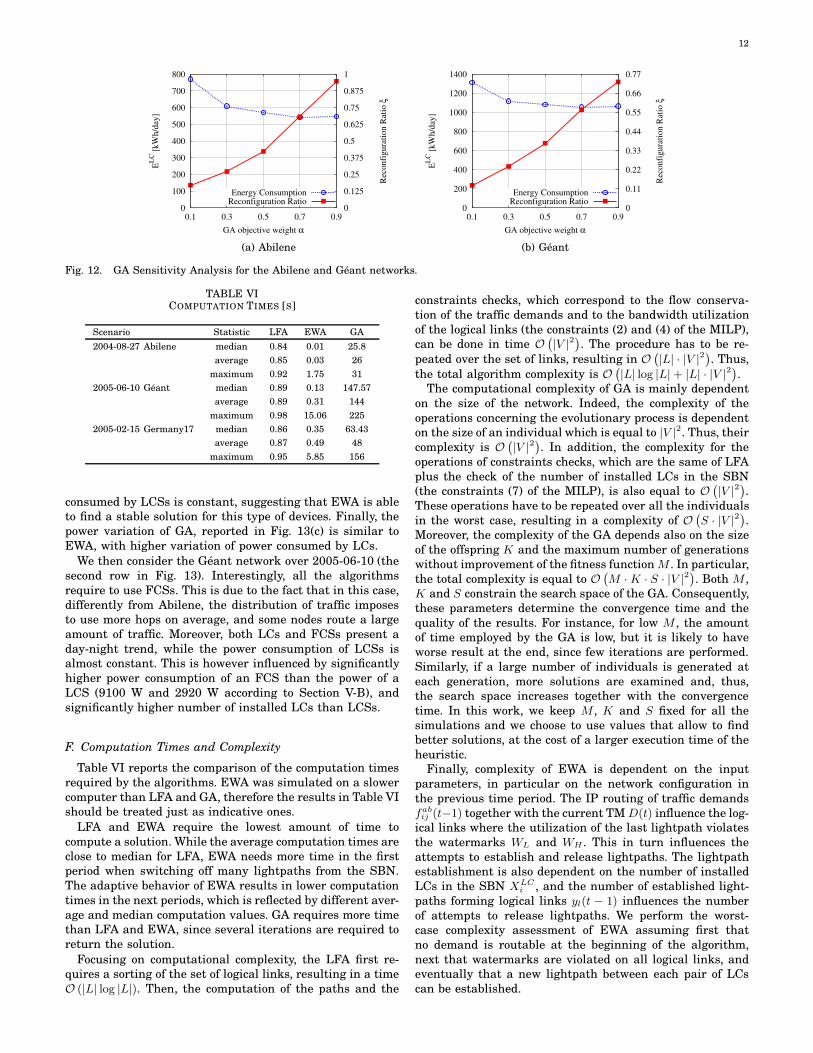
F. Computation Times and Complexity

Table VI reports the comparison of the computation times

required by the algorithms. EWA was simulated on a slower

computer than LFA and GA, therefore the results in Table VI

should be treated just as indicative ones.

LFA and EWA require the lowest amount of time to

compute a solution. While the average computation times are

close to median for LFA, EWA needs more time in the first

period when switching off many lightpaths from the SBN.

The adaptive behavior of EWA results in lower computation

times in the next periods, which is reflected by different aver-

age and median computation values. GA requires more time

than LFA and EWA, since several iterations are required to

return the solution.

Focusing on computational complexity, the LFA first re-

quires a sorting of the set of logical links, resulting in a time

O (|L| log |L|). Then, the computation of the paths and the

constraints checks, which correspond to the flow conserva-

tion of the traffic demands and to the bandwidth utilization

of the logical links (the constraints (2) and (4) of the MILP),

can be done in time O(

|V |2)

. The procedure has to be re-

peated over the set of links, resulting in O(

|L| · |V |2)

. Thus,

the total algorithm complexity is O(

|L| log |L|+ |L| · |V |2)

.

The computational complexity of GA is mainly dependent

on the size of the network. Indeed, the complexity of the

operations concerning the evolutionary process is dependent

on the size of an individual which is equal to |V |2. Thus, their

complexity is O(

|V |2)

. In addition, the complexity for the

operations of constraints checks, which are the same of LFA

plus the check of the number of installed LCs in the SBN

(the constraints (7) of the MILP), is also equal to O(

|V |2)

.

These operations have to be repeated over all the individuals

in the worst case, resulting in a complexity of O(

S · |V |2)

.

Moreover, the complexity of the GA depends also on the size

of the offspring K and the maximum number of generations

without improvement of the fitness functionM . In particular,

the total complexity is equal to O(

M ·K · S · |V |2)

. Both M ,

K and S constrain the search space of the GA. Consequently,

these parameters determine the convergence time and the

quality of the results. For instance, for low M , the amount

of time employed by the GA is low, but it is likely to have

worse result at the end, since few iterations are performed.

Similarly, if a large number of individuals is generated at

each generation, more solutions are examined and, thus,

the search space increases together with the convergence

time. In this work, we keep M , K and S fixed for all the

simulations and we choose to use values that allow to find

better solutions, at the cost of a larger execution time of the

heuristic.

Finally, complexity of EWA is dependent on the input

parameters, in particular on the network configuration in

the previous time period. The IP routing of traffic demands

fabij (t−1) together with the current TMD(t) influence the log-

ical links where the utilization of the last lightpath violates

the watermarks WL and WH . This in turn influences the

attempts to establish and release lightpaths. The lightpath

establishment is also dependent on the number of installed

LCs in the SBN XLCi , and the number of established light-

paths forming logical links yl(t − 1) influences the number

of attempts to release lightpaths. We perform the worst-

case complexity assessment of EWA assuming first that

no demand is routable at the beginning of the algorithm,

next that watermarks are violated on all logical links, and

eventually that a new lightpath between each pair of LCs

can be established.

13

0

50

100

150

200

250

300

00:00 06:00 12:00 18:00 00:00

Po

wer

Co

nsu

mp

tio

n [

kW

]

Time

Line CardsFCSsLCSs

(a) LFA - Abilene

0

50

100

150

200

250

300

00:00 06:00 12:00 18:00 00:00

Po

wer

Co

nsu

mp

tio

n [

kW

]

Time

Line CardsFCSsLCSs

(b) EWA - Abilene

0

50

100

150

200

250

300

00:00 06:00 12:00 18:00 00:00

Po

wer

Co

nsu

mp

tio

n [

kW

]

Time

Line CardsFCSsLCSs

(c) GA - Abilene

0

50

100

150

200

250

300

00:00 06:00 12:00 18:00 00:00

Po

wer

Co

nsu

mp

tio

n [

kW

]

Time

Line CardsFCSsLCSs

(d) LFA - Geant

0

50

100

150

200

250

300

00:00 06:00 12:00 18:00 00:00

Po

wer

Co

nsu

mp

tio

n [

kW

]

Time

Line CardsFCSsLCSs

(e) EWA - Geant

0

50

100

150

200

250

300

00:00 06:00 12:00 18:00 00:00

Po

wer

Co

nsu

mp

tio

n [

kW

]

Time

Line CardsFCSsLCSs

(f) GA - Geant

Fig. 13. Power Breakdown for the Abilene and Geant networks.

We assess each step of the EWA presented in Alg. 3. Ensur-

ing routability of demands over the network requires time

O(

|V |2 · |V |2 log |V |)

, since there are up to |V × V | traffic de-

mands, and establishing of a new logical link for any demand

may influence the routability of all demands, which need to

be sorted (|V |2 log |V |). Sorting of the logical links according

to the utilization of the last lightpath takes O (|L| log |L|).Establishing of necessary lightpaths requires three types

of operations: i) iterations over all the logical links where

the high watermark WH is exceeded (|L|), ii) sorting of the

demands flowing through the logical link (|V |2 log |V |), iii)

possible iterations over all demands flowing through the logi-

cal link (|V |2). Finally the whole procedure has to be repeated

in case a new lightpath is established between any LCs with

the total number of LCs installed in the network defined as

R =∑

i∈VXLC

i . The overall complexity of establishing of

the necessary lightpaths (consisting of the above three types

of operations) is O(

|L| ·(

|V |2 log(|V |) + |V |2)

·R2)

(see [41]).

Releasing unnecessary lightpaths takes O (G · |L| log |L|),where G =

∑

l∈L yl(t − 1) denotes the number of estab-

lished lightpaths in the previous time period, and |L| log |L|accounts for the fact that releasing each single lightpath

forces sorting of logical links. The overall complexity of EWA

(Alg. 3) can be therefore estimated in the worst case as

O(

|V |4 log |V |+ |L|R2 |V |2 log |V |+G |L| log |L|)

.

In conclusion, all algorithms present complexity that

scales at least as |V |2. Moreover, complexity of both GA and

EWA depends on the input parameters, which can be used

to trade between quality of results and computation time.

Finally, complexity of LFA is independent from the input

parameters, and it is fixed given the SBN.

G. Monetary Savings

Finally, we have estimated the impact of our heuristics

on the monetary cost needed to power the network. In

particular, we have selected the day 2004-08-27 for Abilene,

the day 2005-06-10 for Geant, and the day 2005-02-15 for

Germany17. By assuming that the same daily traffic profile

TABLE VIIYEARLY MONETARY COST [Ke]

Abilene Geant Germany17

ALL ON 280 526 260

LFA 145 (-48%) 166 (-69%) 186 (-28%)

EWA 52 (-81%) 110 (-79%) 161 (-38%)

GA 55 (-80%) 112 (-79%) 147 (-43%)

is repeated over the whole year we have computed the

total energy consumed by the network in a year, and the

corresponding electricity costs.5 A cost of 0.0936 e per kWh

is assumed, based on current statistics of electricity prices

in Europe [47]. Table VII reports the costs for the three

algorithms. Although not being the main focus of this paper,

percentage savings with respect to an always on solution

are reported in the parenthesis. Considering the Abilene

network, an always on solution requires 280000 e per year.

With LFA this amount can be almost halved, while with

EWA and GA savings larger than 80% can be achieved, with

52000 e required to run the network with EWA. Higher

savings can be achieved for the Geant network, with the

lowest amount of electricity required by the EWA algorithm.

Finally, savings between 28% and 43% are achieved with the

Germany17 network. These results corroborate our intuition

that reducing power consumption is of significant benefit also

for reducing the associated monetary cost.

VIII. DISCUSSION AND IMPLEMENTATION ISSUES

Power savings and amount of reconfigured traffic depend

on the traffic variation over time. We varied the load in

Section VII-C, but the rate of traffic changes plays also

an important role. The algorithms (especially EWA) are

designed for typical day-night traffic variation in a backbone

network. Traffic in this kind of networks is smooth due to

aggregation of hundreds of end-to-end flows. Extraordinary

and large peaks of traffic are unlikely, and caused by e.g.,

5Weekend days may further decrease the electricity consumption.

14

natural disasters or terrorist attacks, but also transmission

of multiple grid jobs. They may reduce the opportunity for

putting devices into sleep mode, and in such cases, we expect

lower power savings with a higher amount of reconfigured

traffic. Besides, these situations may also result in network

overload if the devices that were put into sleep mode cannot

be awakened fast enough, or if the network is improperly di-

mensioned. Lastly, the algorithms may fail to find a suitable

network configuration for supporting these peaks of traffic,

which may impair the network availability. These issues and

the exact domain of validity of the algorithms with respect

to traffic dynamics have not been studied in this paper, and

are left for future work.

In our case, we have evaluated our heuristics over two

weekend days and two working days (for the Geant and

Abilene networks), and one day for the Germany17 network.

We have selected these days, because of their typical day-

night traffic variation in a backbone network. We assume

that in normal conditions, traffic in the network varies with

a similar trend, and so the power saving and the amount of

reconfigured traffic would be similar. Moreover, the adopted

time granularity (one TM every 15 minutes) is sufficient to

mimic the real traffic variation in the network.

Furthermore, there are different implementation issues

that need to be taken into account when introducing the

proposed heuristics into the networks. First of all, the fea-

ture of remote activation and deactivation of the LCs, and

potentially also LCSs and FCSs has to be integrated into

IP routers. Although commercial routers available today do

not posses this functionality yet, their vendors work on its

implementation [48]. In general, estimating the time that is

needed to power up a LC in an IP-over-WDM network is not

trivial. However, the 3 microseconds needed to wake up a

10 Gbps link in the emerging 802.3az standard [27] makes

us believe that the wake-up process will be quick enough to

follow the traffic variation.

Additionally, in the case of a centralized controller, it is

necessary to consider the time needed to run the algorithm

(the approximate time is indicated in Table VI, considering

that the algorithms’ implementation is not explicitly opti-

mized to be time effective) and the time to disclose the new

network configuration to all the nodes. This can be done

using a new signaling mechanism or an already existing

one. For instance, the computed network configuration can

be put inside LSA packets, assuming the existing MPLS as

the control plane [30]. Alternatively, the algorithms can be

run in a distributed manner at each node, which requires

prior collection of the necessary global data.

Lastly, additional time is needed to reconfigure the net-

work, first switching on new equipment, then making sure

that all the traffic has been rerouted, and eventually switch-

ing off idle equipment. The make-before-break mechanism

[49] can be used for this purpose.

IX. CONCLUSION

We have targeted the reduction of power consumption

in IP-over-WDM networks, by selectively turning off LCs

during periods of low traffic. In particular, we have first

formulated the Multi-Period Power-Aware Logical Topology

Design problem (MP-PA-LTD) as an optimization problem.

Then, we have proposed three different heuristics to solve

the MP-PA-LTD, namely LFA, GA and EWA. The LFA tar-

gets the minimization of the number of logical links in the

network, while both GA and EWA work on single lightpaths.

Differently from the previous work, we take into account the

amount of traffic which is reconfigured in the network.

We have evaluated our algorithms over a wide set of

network scenarios taking as realistic parameters as possible.

Our results indicate that switching off LCs is of great benefit

to reduce the power consumption of the network. Moreover,

both GA and EWA are able to wisely trade between power

and reconfigured traffic, and this trade-off can be controlled

by a proper setting of the input parameters. Then, we have

shown that with our heuristics the traffic load impacts

the power consumption, but only marginally the associated

reconfiguration ratio. Additionally, also the overprovisioning

of the SBN has a limited impact on the reconfiguration ratio.

Finally, we have shown that reducing power consumption is

of significant benefit for reducing the associated monetary

cost.

In conclusion, our results indicate that large savings are

possible while keeping the reconfigured traffic low. This is

true especially for the GA and EWA algorithms, which are

designed to switch off single lightpaths rather than full

logical links. Moreover, the average computation time below

0.5 s (median below 0.35 s) makes the EWA a candidate to

be implemented in operational core networks.

ACKNOWLEDGMENT

This paper is dedicated to the memory of prof. Fabio Neri,

who suddenly passed away in April 2011. Fabio was a full

professor at Politecnico di Torino, and his suggestions on

optical networks helped us in the initial steps of this work.

The research leading to these results has received funding

from the European Union Seventh Framework Programme

(FP7/2007-2013) under grant agreement n. 257740 (Network

of Excellence “TREND”).

REFERENCES

[1] M. Pickavet, W. Vereecken, S. Demeyer, P. Audenaert, B. Ver-meulen, C. Develder, D. Colle, B. Dhoedt, and P. Demeester,“Worldwide Energy Needs for ICT: the Rise of Power-AwareNetworking,” in Proc. of the ANTS, Bombay, India, December2008.

[2] C. Lange, D. Kosiankowski, C. Gerlach, F. Westphal, andA. Gladisch, “Energy Consumption of Telecommunication Net-works,” in Proc. of the ECOC, Vienna, Austria, September 2009.

[3] E. Bonetto, L. Chiaraviglio, D. Cuda, F. Idzikowski, and F. Neri,“Exploiting Traffic Dynamics in Power-Aware Logical TopologyDesign,” in Proc. of the ECOC, Geneva, Switzerland, September2011.

[4] M. Pioro and D. Medhi, Routing, Flow, and Capacity Design inCommunication and Computer Networks. Morgan Kaufmann,2004.

[5] B. Mukherjee, Optical WDM networks. Springer, 2006.[6] D. Banerjee and B. Mukherjee, “Wavelength-routed optical

networks: linear formulation, resource budgeting tradeoffs, anda reconfiguration study,” Transactions on Networking, vol. 8,no. 5, pp. 598–607, October 2000.

[7] B. Ramamurthy and A. Ramakrishnan, “Virtual topology re-configuration of wavelength-routed optical wdm networks,” inProc. of the GLOBECOM, San Francisco, USA, November 2000.

[8] H. Zhu, H. Zang, K. Zhu, and B. Mukherjee, “Dynamic trafficgrooming in WDM mesh networks using a novel graph model,”in Proc. of the GLOBECOM, Taipei, Taiwan, November 2002.

[9] I. Baldine and G. Rouskas, “Traffic adaptive wdm networks: astudy of reconfiguration issues,” Journal of Lightwave Technol-ogy Networking, vol. 19, no. 4, pp. 433–455, 2001.

[10] G. Rouskas and M. Ammar, “Dynamic reconfiguration in mul-tihop WDM networks,” Journal of High Speed Networks, vol. 4,pp. 221–238, 1995.

15

[11] J.-F. Labourdette, G. Hart, and A. Acampora, “Branch-exchangesequences for reconfiguration of lightwave networks,” Transac-tions on Networking, vol. 42, no. 10, pp. 2822–2832, October1994.

[12] M. Kato and Y. Oie, “Reconfiguration algorithms based onmeta-heuristics for multihop wdm lightwave networks,” in Proc.of the ICC, New Orleans, USA, June 2000.

[13] H. Takagi, Y. Zhang, and X. Jia, “Virtual topology reconfigu-ration for wide-area wdm networks,” in Proc. of the ICCCAS,Chengdu, China, June 2002.

[14] A. Narula-Tam and E. Modiano, “Dynamic load balancing forWDM-based packet networks,” in Proc. of the INFOCOM, Tel-Aviv, Israel, March 2000.

[15] N. Farzaneh and M. Moghaddam, “Virtual topology reconfigu-ration of WDM optical networks using fuzzy logic control,” inProc. of the International Symposium on Telecommunications,Teheran, Iran, November 2008.

[16] N. Skorin-Kapov, P. Pavon-Marino, B. Garcia-Manrubia, andR. Aparicio-Pardo, “Scheduled Virtual Topology Design UnderPeriodic Traffic in Transparent Optical Networks,” in Proc. ofthe BROADNETS, Madrid, Spain, September 2009.

[17] R. Aparicio-Pardo, P. Pavon-Marino, N. Skorin-Kapov,B. Garcia-Manrubia, and J. Garcia-Haro, “Algorithms forvirtual topology reconfiguration under multi-hour traffic usingLagrangian relaxation and Tabu Search approaches,” in Proc.of the ICTON, Munich, Germany, June 2010.

[18] R. Aparicio-Pardo, B. Garcia-Manrubia, N. Skorin-Kapov, andP. Pavon-Marino, “Heuristic approaches for periodic reconfig-uration of lightpath-based networks under multi-hour traffic,”Journal of Networks, vol. 7, no. 5, pp. 800–811, May 2012.

[19] R. Aparicio-Pardo, N. Skorin-Kapov, P. Pavon-Marino, andB. Garcia-Manrubia, “(non)-reconfigurable virtual topology de-sign under multi-hour traffic in optical networks,” Transactionson Networking, vol. 20, no. 5, pp. 1567–1580, October 2012.

[20] P. Pavon-Marino, R. Aparicio-Pardo, B. Garcia-Manrubia, andN. Skorin-Kapov, “Virtual topology design and flow routing inoptical networks under multi-hour traffic demand,” PhotonicNetwork Communications, vol. 19, no. 1, pp. 42–54, February2010.

[21] P. Pavon-Marino, B. Garcia-Manrubia, and R. Aparicio-Pardo,“Multi-hour network planning based on domination betweensets of traffic matrices,” Computer Networks, vol. 55, no. 3, pp.665–675, February 2011.

[22] A. Gencata and B. Mukherjee, “Virtual-topology adaptation forWDM mesh networks under dynamic traffic,” Transactions onNetworking, vol. 11, no. 2, pp. 236–247, 2003.

[23] P. N. Tran and U. Killat, “Dynamic reconfiguration of logicaltopology for WDM networks under traffic changes,” in Proc. ofthe Network Operations and Management Symposium (NOMS),Salvador, Brazil, April 2008, pp. 279–286.

[24] N. Sengezer and E. Karasan, “Multi-layer virtual topologydesign in optical networks under physical layer impairmentsand multi-hour traffic demand,” Journal of Optical Communi-cations and Networking, vol. 4, no. 2, pp. 78–91, February 2012.

[25] P. N. Tran and U. Killat, “Distributed algorithm for dynamiclogical topology reconfiguration in IP over WDM networks,” inProc. of the Symposium on Computers and Communications(ISCC), Sousse, Tunisia, July 2009, pp. 748–756.

[26] F. Idzikowski, S. Orlowski, C. Raack, H. Woesner, and A. Wolisz,“Dynamic routing at different layers in IP-over-WDM networks– maximizing energy savings,” Optical Switching and Network-ing, Special Issue on Green Communications, vol. 8, no. 3, pp.181–200, July 2011.

[27] R. Bolla, R. Bruschi, F. Davoli, and F. Cucchietti, “Energy Effi-ciency in the Future Internet: A Survey of Existing Approachesand Trends in Energy-Aware Fixed Network Infrastructures,”IEEE Communications Surveys & Tutorials, vol. 13, no. 2, pp.223–244, 2011.

[28] Y. Zhang, P. Chowdhury, M. Tornatore, and B. Mukherjee,“Energy Efficiency in Telecom Optical Networks,” IEEE Com-munications Surveys & Tutorials, vol. 12, no. 4, pp. 441–458,2010.

[29] A. P. Bianzino, C. Chaudet, D. Rossi, and J.-L. Rougier, “ASurvey of Green Networking Research,” IEEE CommunicationsSurveys & Tutorials, vol. 14, no. 1, pp. 3–20, 2012.

[30] M. Zhang, C. Yi, B. Liu, and B. Zhang, “GreenTE: Power-aware

traffic engineering,” in Proc. of the International Conference onNetwork Protocols (ICNP), Kyoto, Japan, October 2010.

[31] R. Bolla, R. Bruschi, A. Cianfrani, and M. Listanti, “EnablingBackbone Networks to Sleep,” IEEE Network, vol. 25, no. 2, pp.26–31, 2011.

[32] H. Yonezu, K. Kikuta, D. Ishii, S. Okamoto, E. Oki, and N. Ya-manaka, “QoS aware energy optimal network topology designand dynamic link power management,” in Proc. of the ECOC,Torino, Italy, September 2010.

[33] A. P. Bianzino, C. Chaudet, F. Larroca, D. Rossi, and J.-L.Rougier, “Energy-aware routing: a reality check,” in Proc. ofthe GLOBECOM workshop on Green Communications, Miami,USA, December 2010.

[34] Y. Zhang, M. Tornatore, P. Chowdhury, and B. Mukherjee, “En-ergy optimization in IP-over-WDM networks,” Optical Switch-ing and Networking, Special Issue on Green Communications,vol. 8, no. 3, pp. 171–180, July 2011.

[35] M. Caria, M. Chamania, and A. Jukan, “A comparative perfor-mance study of load adaptive energy saving schemes for IP-over-WDM networks,” Journal of Optical Communications andNetworking, vol. 4, no. 3, pp. 152–164, March 2012.

[36] A. P. Bianzino, L. Chiaraviglio, and M. Mellia, “GRiDA: a greendistributed algorithm for backbone networks,” in Proc. of theGreenCom, online, September 2011.

[37] ——, “Distributed algorithms for green IP networks,” in Proc.of the INFOCOM workshop on Communications and Controlfor Sustainable Energy Systems, Orlando, USA, March 2012.

[38] A. Coiro, F. Iervini, and M. Listanti, “Distributed and adaptiveinterface switch off for internet energy saving,” in Proc. of theICCCN, Maui, USA, July 2011.

[39] L. Chiaraviglio, M. Mellia, and F. Neri, “Minimizing ISP Net-work Energy Cost: Formulation and Solutions,” Transactionson Networking, vol. 20, no. 2, pp. 463–476, April 2012.

[40] A. Ahmad, A. Bianco, E. Bonetto, D. Cuda, G. G. Castillo,and F. Neri, “Power-aware logical topology design heuristics inwavelength-routing networks,” in Proc. of the ONDM, Bologna,Italy, February 2011.

[41] F. Idzikowski, E. Bonetto, and L. Chiaraviglio, “EWA – anadaptive algorithm using watermarks for energy saving in IP-over-WDM networks,” Technical University of Berlin, Telecom-munication Networks Group, Tech. Rep. TKN-12-002, May2012.

[42] J. Chabarek, J. Sommers, P. Barford, C. Estan, D. Tsiang, andS. Wright, “Power awareness in network design and routing,”in Proc. of the INFOCOM, Phoenix, USA, April 2008.

[43] Zuse-Institut Berlin, “Sndlib: library of test instances for sur-vivable fixed telecommunication network design,” http://sndlib.zib.de/home.action, February 2012.

[44] Cisco, “Cisco CRS-1 Production Brochure,” http://www.cisco.com/en/US/prod/collateral/routers/ps5763/prodbrochure0900aecd800f8118.pdf, October 2008.

[45] F. Idzikowski, “Power consumption of network elements in IPover WDM networks,” Technical University of Berlin, Telecom-munication Networks Group, Tech. Rep. TKN-09-006, July2009.

[46] R. Hulsermann, M. Gunkel, C. Meusburger, and D. A. Schupke,“Cost modeling and evaluation of capital expenditures in op-tical multilayer networks,” Journal of Optical Networking,vol. 7, no. 9, pp. 814–833, 2008.

[47] European Commission, “Eurostat database,” http://epp.eurostat.ec.europa.eu/, February 2012.

[48] M. Yamada, T. Yazaki, N. Matsuyama, and T. Hayashi, “Power-efficient multi-layer traffic networking: Design and evaluation,”in Proc of the ICC workshop on Green Communications, Dres-den, Germany, June 2009.

[49] A. Farrel and I. Bryskin, GMPLS Architecture and Applica-tions. Morgan Kaufmann, 2006.

APPENDIX A

SUMMARY OF THE NOTATION

Table VIII contains explanation of all the symbols used in

this work.

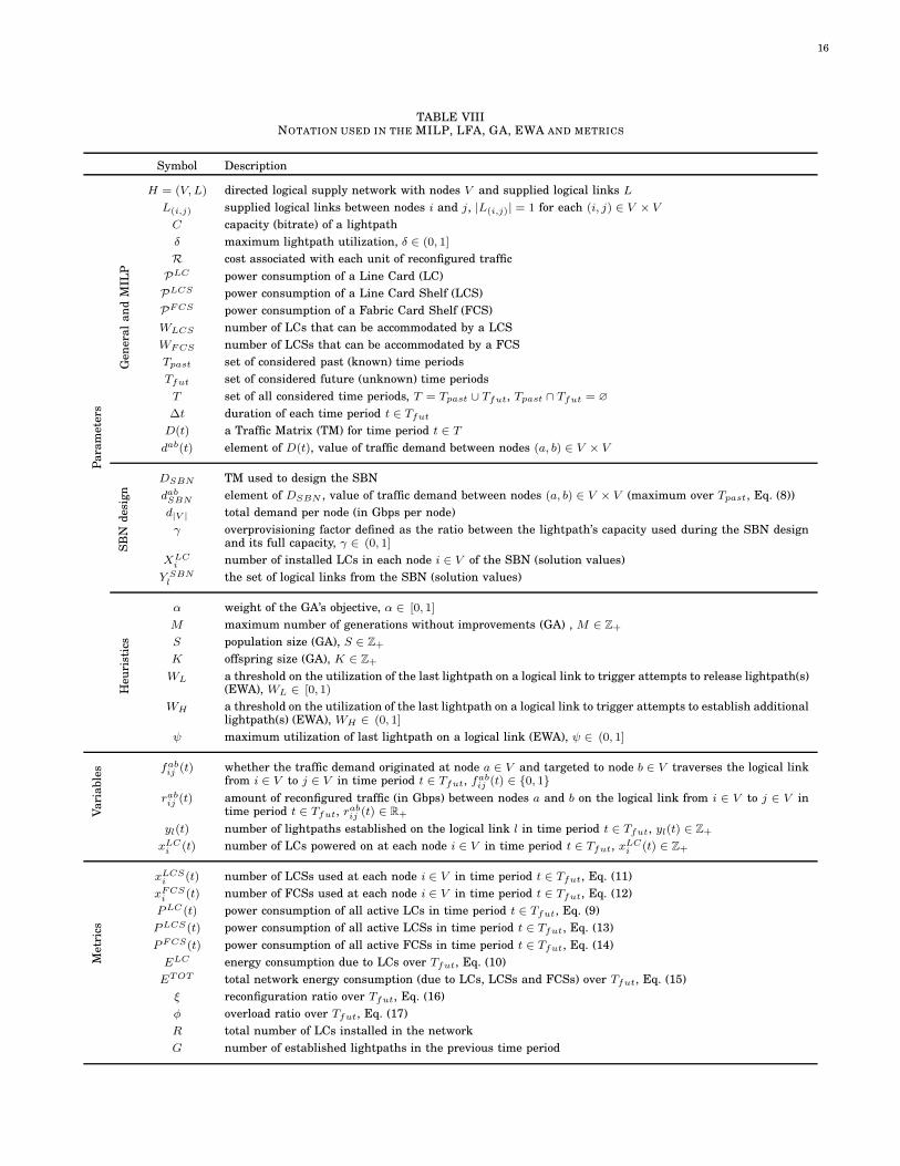
16

TABLE VIIINOTATION USED IN THE MILP, LFA, GA, EWA AND METRICS

Symbol Description

Pa

ram

ete

rs

Gen

era

la

nd

MIL

P

H = (V, L) directed logical supply network with nodes V and supplied logical links L

L(i,j) supplied logical links between nodes i and j, |L(i,j)| = 1 for each (i, j) ∈ V × V

C capacity (bitrate) of a lightpath

δ maximum lightpath utilization, δ ∈ (0, 1]

R cost associated with each unit of reconfigured traffic

PLC power consumption of a Line Card (LC)

PLCS power consumption of a Line Card Shelf (LCS)

PFCS power consumption of a Fabric Card Shelf (FCS)

WLCS number of LCs that can be accommodated by a LCS

WFCS number of LCSs that can be accommodated by a FCS

Tpast set of considered past (known) time periods

Tfut set of considered future (unknown) time periods

T set of all considered time periods, T = Tpast ∪ Tfut, Tpast ∩ Tfut = ∅

∆t duration of each time period t ∈ Tfut

D(t) a Traffic Matrix (TM) for time period t ∈ T

dab(t) element of D(t), value of traffic demand between nodes (a, b) ∈ V × V

SB

Nd

esi

gn

DSBN TM used to design the SBN

dabSBN element of DSBN , value of traffic demand between nodes (a, b) ∈ V × V (maximum over Tpast, Eq. (8))

d|V | total demand per node (in Gbps per node)

γ overprovisioning factor defined as the ratio between the lightpath’s capacity used during the SBN designand its full capacity, γ ∈ (0, 1]

XLCi number of installed LCs in each node i ∈ V of the SBN (solution values)

Y SBNl

the set of logical links from the SBN (solution values)

Heu

rist

ics

α weight of the GA’s objective, α ∈ [0, 1]

M maximum number of generations without improvements (GA) , M ∈ Z+

S population size (GA), S ∈ Z+

K offspring size (GA), K ∈ Z+

WL a threshold on the utilization of the last lightpath on a logical link to trigger attempts to release lightpath(s)(EWA), WL ∈ [0, 1)

WH a threshold on the utilization of the last lightpath on a logical link to trigger attempts to establish additionallightpath(s) (EWA), WH ∈ (0, 1]

ψ maximum utilization of last lightpath on a logical link (EWA), ψ ∈ (0, 1]

Va

ria

ble

s fabij (t) whether the traffic demand originated at node a ∈ V and targeted to node b ∈ V traverses the logical linkfrom i ∈ V to j ∈ V in time period t ∈ Tfut, f

abij (t) ∈ {0, 1}

rabij (t) amount of reconfigured traffic (in Gbps) between nodes a and b on the logical link from i ∈ V to j ∈ V intime period t ∈ Tfut, r

abij (t) ∈ R+

yl(t) number of lightpaths established on the logical link l in time period t ∈ Tfut, yl(t) ∈ Z+

xLCi (t) number of LCs powered on at each node i ∈ V in time period t ∈ Tfut, x

LCi (t) ∈ Z+

Metr

ics

xLCSi (t) number of LCSs used at each node i ∈ V in time period t ∈ Tfut, Eq. (11)

xFCSi (t) number of FCSs used at each node i ∈ V in time period t ∈ Tfut, Eq. (12)

PLC(t) power consumption of all active LCs in time period t ∈ Tfut, Eq. (9)

PLCS(t) power consumption of all active LCSs in time period t ∈ Tfut, Eq. (13)

PFCS(t) power consumption of all active FCSs in time period t ∈ Tfut, Eq. (14)

ELC energy consumption due to LCs over Tfut, Eq. (10)

ETOT total network energy consumption (due to LCs, LCSs and FCSs) over Tfut, Eq. (15)

ξ reconfiguration ratio over Tfut, Eq. (16)

φ overload ratio over Tfut, Eq. (17)

R total number of LCs installed in the network

G number of established lightpaths in the previous time period