Education and Signaling in Hong Kong

By

Lui Siu Hei

07005407

Applied Economics Major

An Honours Degree Project Submitted to the

School of Business in Partial Fulfilment

of the Graduation Requirement for the Degree of

Bachelor of Business Administration (Honours)

Hong Kong Baptist University

Hong Kong

April 2009

Acknowledgement

I want to give a big thanks to Dr. Y.C. Ng for her patience and her every help when I was

struggled in doing this paper. From model specification to computer programs, this paper is

impossible to finish without her help. It’s precious to have her guidance. I also want to thank my

family including my girlfriend Fanny Lok. I am always overwhelmed by their unlimited love and

support. I do have to appreciate my schoolfellows especially the “Econmates” who like the battle

companions during these last days in school.

Content:

I. Abstract P.1

II. Introduction P.2

III. Literature Review P.6

IV. Methodology P.11

V. Data P.16

VI. Empirical Results P.17

VII. Limitations P.26

VIII. Conclusion P.28

Reference

1

I. Abstract

This paper investigates the Hong Kong Labor market for the validity of the human capital

theory as well as the screening hypothesis by comparing the return of education of the employed

as the presumed screened and the self-employed as presumed unscreened. The Mincerian

earnings equation is used to estimate the return of education of the screened jobs and the

unscreened jobs by genders. And Heckman two-step procedure is introduced to correct the

selection bias of the earnings functions. The results shows that human capital theory does explain

part of the return of education and the rest of it can be explained by the “signal” suggested by

screening hypothesis.

2

II. Introduction

Many empirical labor economic studies have confirmed a strong positive relationship

between education levels and earnings of an individual. However, different economists have

different arguments on the causes of the way that higher education level leads to higher earnings.

There are two major opinions on the causes of the positive relationship: human capital theory

and screening hypothesis.

The human capital theory suggests education is a form of investment in human capital.

Becker (1993) states that knowledge, experiences, skills and health are different kinds of human

capital which are not able to separate from the individual. Education directly adds to productivity

and expenditure on education, training, medical care, etc, are in fact investments in human

capital that generate future returns such as raised earnings. Education as a kind of investment

endows an individual with more knowledge and better skills that positively related to one’s job-

related productivity. Therefore, employee with higher education level implies he/she would be

better equipped than his/her co-worker who has lower education level regardless other factors

determines their earnings. Individuals will only enter college if they can generate higher net

lifetime income.

3

Employee with higher education level in general earns more because of his/her higher

productivity endowed by education. In the view of employers, employees with higher education

level and hence higher productivity should be rewarded and worth higher salaries. The human

capital theory also suggests that education is an important source of economic growth (Denison,

1985) because it improves the quality as well as productivity of the labor force. Therefore

investment in education benefits to the whole society and government may have to invest heavily

on it.

Different from human capital theory, the screening hypothesis suggests that education is

not a kind of investment on human capital actually. The screening hypothesis suggests that

education is only or primarily used as a screening device that sort individua ls according to how

much should be paid to the individuals from highest to the least. Moreover, the screening

hypothesis supports that education is a filter that individuals have less talent would be screened

out or leave the education system as cost of the education outweigh benefit of it and those

remained that is better talented would be advanced to a higher level. Eventually, the higher the

education level an individual has, the better the talent he/she is.

In the point of view of employers, education is only a “signal”. When making hiring

decision to an individual, employer does not have full information about a candidate even though

4

the employer have interviewed and/or tested the candidate several times. The employer faces

risks of employing an individual with low productivity. In order to increase the probability of

hiring a suitable one, employer may simply use “signals” to determine whether to hire an

individual or not. As education level is a reliable signal to reflect the connate ability of an

individual, it is reasonable to believe that the more productive individual is the one who attain

highest education level (Riley, 1979). Therefore, it is the “sheepskin” that is rewarded rather

than the productivity which is suggested by the human capital theory (Layard & Psacharopoulos,

1974 and Chiswick, 1973).

The screening hypothesis also suggests that most job skills are not obtained from

education but are acquired by on-the-job training (Thurow, 1975). And what employers want is

the fastest learner with least training cost. Therefore, education is used by individuals as a self-

selection process that individuals signal their trainability. Slower learners would sift out as their

opportunity cost of achieve higher education is greater. The screening hypothesis implies

education yield higher private return to individuals than social benefits as education does not

really increase the productivity of workers which may result in over- investment in education

(Chatterji, Seaman & Singell, 2003) and hence suggests government to save money to invest in

other areas to generate higher return instead of invest so heavy in education and ask government

to simplify the screening device such as public examinations, IQ tests, etc.

5

To provide stronger evidence for determine the human capital theory and screening

hypothesis, a less regulated labor market should be investigated. It is because the higher the

regulated labor market the less the difference of wages as wages setting is centralized or

unionized (Addison & Siebert, 1997) which in turn provide less evidence for determining the

human capital theory and the screening hypothesis. Therefore, the labor market in Hong Kong

would be investigated in this project after Heywood and Wei (2004) with the same reasons that

as Hong Kong is one of the most competitive labor markets with least labor legislation

restrictions when compare to other developed cities like Singapore. Therefore the effect of

education to earnings of labors would be better reflected.

A common method to investigate this topic is to compare the return of education on

earnings of the presumed screened group and that of the presumed unscreened group which is

also the method used in this project and it will discuss later in this paper. And as the earnings

functions estimation of males and females are different, the samples would then separated by

gender to evaluate.

6

III. Literature review

Education increases earnings. Human capital theory suggests the reason of increase in

earnings because of education directly increases productivity of an individual. However,

supporters of screening hypothesis argue that education only or primarily act as a signal to the

learning speed and ability of the individual. The debate between the two thoughts still exists.

Although many economists have done many great works on the issue, neither side can reason

down another. Some empirical studies support the former one and others support the later. All

these papers aim to investigate the true reason behind the positive relationship between educa tion

and earnings. Table 1 below summarizes results of some literatures.

Table 1

Authors Country/city

studied Supporting

side

Riley, 1979 United States S

Tao, 2006 United States H

Chatterji, Seaman & Singell, 2003 United Kingdom S

Miller & Volker, 1984 Australia S

Groot & Oosterbeek, 1994 Dutch H

Gullason, 1998 Global S

Heywood & Wei, 2004 Hong Kong S

S: Examines the screening hypothesis,

H: Examines the human capital theory

As noticed in Table 1, different literatures support different views. In fact, different

economists use different methods to investigate the issue.

7

Riley (1979) studies the U.S. labor market, and compares the presumed screened

occupations versus the presumed unscreened occupations. He finds that the occupations with low

earnings functions and high mean education is better fitted to the presumed unscreened

occupations. This result supports the screening hypothesis as return on earnings of education for

unscreened occupations is less than that of screened occupations.

Tao (2006) also investigates the U.S. labor market. He wonders that if the extreme

screening hypothesis is true, there would be no significant different of productivity and hence

life-time earnings for those who has the same innate ability no matter the individual enter college

or not as he/she may have same productivity. Tao finds that the human capital accumulation

factor over time has significant impact on the earnings equation. And this finding supports the

human capital theory over the extreme screening hypothesis as it implies that human capital

actually adds to productivity.

Chatterji, Seaman and Singell (2003) study the U.K. labor market by comparing the

return of education of those presumed screened employees with those presumed unscreened self-

employed. They find that the “signal” has a positive rate of return to earnings of workers. When

it is eliminated from the earnings equation, the return of education is underestimated. That means

8

the signaling effect actually enhance the return to education and the authors believe that the

signaling does occur in U.K., especially females rely more on it than males.

Miller and Volker (1984) compare the college graduates of two majors: economics and

science in Australia, to see whether there is significant different in starting salaries of graduates

who work in relevant field of their studies compare to those who work in other fields. They

conclude that the screening hypothesis alive and well in Australia as for the economics majored

graduates, there is no significant different in earnings between those who work in relevant fields

and those who are not. However, the conclusion is not that strong because the salaries of the

science majored graduates who work for relevant field is significantly higher than those who

work for other fields, especially for the males graduates.

Groot and Oosterbeek (1994) investigate the case in Dutch where has a flexible education

system. This education system allows Groot and Oosterbeek to divide the education years into

effective years, repeated years, skipped years, inefficient years and dropout years and include

these years separately into the earnings function. The screening hypothesis assumes that

individual who is signaled as a quicker learner should be rewarded and skipped years, which is

the number of years that an individual “jump over” because of his/her outstanding academic

performance, imply an individual has greater trainability and instead repeated years imply less

9

trainability. However the result overthrows the screening hypothesis by concluding that there are

a negative effect of skipped years and a neutral effect of repeated years to earnings. Besides, the

result build an even stronger stand for human capital by demonstrate the positive effect of

dropout years to earnings, which is the number of years that an individual studied but dropped

out without a certificate. The positive relationship contradicts to the “sheepskin” effect of the

screening hypothesis.

Gullason (1998) studies the screening hypothesis versus the human capital theory from a

global perspective. He compares two different formulated variables of years of schooling:

exogenous formulated and endogenous formulated. He finds that the exogenous formulated one

is able to explain the earnings functions but the endogenous formulated does not. And it implies

that employers simply use education as a device to assess the productivity of the candidates. It is

in the line of the screening hypothesis that employers do not has full information of the potential

employees and instead using education level as a indicator to determine the hiring decision.

Heywood and Wei (2004) investigate the case in Hong Kong which has a highly

competitive labor market. They separate the labor market into employed which is presumed

screened group and self-employed which is presumed unscreened group. And compare the return

to earnings of education levels either attended or completed. They conclude that the return on

10

education levels of presumed unscreened (self-employed) group is significantly smaller when

compare to the presumed screened (employed) group. Moreover, the result refutes the human

capital as the increase in return of education on the presumed screened group is concentrated on

the completed rather than the attended level which in turn is actually the “sheepskin” effect.

To conclude, it is unable to simply summarize neither the human capital theory nor the

screening hypothesis stand out. As Heywood and Wei (2004) mentioned that different cultures,

institutions and nature of labor markets may result in different evidences of either sides of

opinion and I will follow their work investigate the case in Hong Kong.

11

IV. Methodology

As mentioned before, Heywood and Wei (2004) investigated the labor market in Hong

Kong by separating the presumed unscreened and the presumed screened. The reason behind is

that the self-employed group need not to be screened by employers which the employed does.

This method is adopted in this project. The sample is divided into self-employed which is

presumed unscreened and employed which is presumed screened. Then the two samples are

estimated by semi- log earnings equations separately taking into account of the self-selection bias

of being self-employed versus being employed. The return of education in earnings for females

and males is believed to be different. The earnings function is then separated by gender, in order

to estimate whether signaling effect exists in different genders or not. And if it exists, which

gender would be stronger affected.

The Mincerian earnings equation (Mincer, 1974) is used

For the employed sample:

Lnmearn = β0 + β1(male) + β2(mar) + β3(exp) + β4(exp2) +

β5(lowsec) + β6(upsec) + β7(postsec) + β8(univ) + ε

For the self-employed sample:

Lnmearn = γ0 + α1(male) + γ2(mar) + γ3(exp) + γ4(exp2) +

γ5(lowsec) + γ6(upsec) + γ7(postsec) + γ8(univ) + µ

12

where: Lnmearn = nature log monthly earnings of the observed individual, which is the dependent variable that when independent variable change by 1 unit, the βs and γs will

indicate the changes in monthly earnings in a percentage term.

β0 = constant term for the employed sample

γ0 = constant term for the self-employed sample

male = dummy variable of whether the respondent is male or not

mar = dummy variable of whether the respondent married or not

exp = years of experience of the respondent in labor market which is calculated by age

minus 6 and the number of years of schooling

exp2 = years of experience of the respondent in labor market which is calculated by age minus 6 and the number of years of schooling squared

lowsec = dummy variable of the highest education attended is lower secondary level

upsec = dummy variable of the highest education attended is upper secondary level

postsec = dummy variable of the highest education attended is postsecondary level

univ = dummy variable of the highest education attended is university or above levels

The reference for the highest education level attended is primary level or lower which is

omitted to act as conditions to be compared in the regression. ε and µ = random error

terms which may also capture a selection bias that will talk about later.

Heckman (1979) mentions that using non-randomly selected samples to estimate

behavioral relationships as an ordinary specification would cause sample selection bias. In this

project, it is clear that the employed and self-employed themselves are non-randomly selected

and hence selection bias may be an issue. As the choice of individuals to be employed or self-

employed is endogenous which means individuals may have different characteristics making

him/her more likely to be self-employed. These characteristics are not included in the estimation

13

of the earnings function (De Wit & Van, 1989). The value of the omitted characteristics can be

estimated and included as regressor to eliminate the bias (Heckman, 1979). Therefore,

Heckman’s two step procedure is adopted to capture the bias. The basic idea is:

Firstly, a probit regression for capturing the characteristics of self-employed is estimated:

P(Self) = Φ(Zi)

where: Zi = α0 + α1(A40) + α2(MT7) + α3(OSE) + α4(HKB)

Self indicates self-employed (Self = 1 if the individual is self-employed and Self = 0

otherwise). Φ is the cumulative distribution function. α0 is the constant term.

As Heywood and Wei (2004) mentions that as experiences and personal network are

needed, people who are more mature and/or reside in Hong Kong a longer period would be more

likely to be self-employed. Also certain positions and occupations are more likely to be self-

employed. Therefore, three independent dummy variables are included which indicate whether

an individual aged equal to or above 40 or not, reside in Hong Kong for 7 years or more or not

and is born in Hong Kong or not. Moreover, a dummy variable OSE is included to indicate

whether an individual is in certain positions and occupations indicating that they are more likely

to be self-employed. Those positions and occupations are small business manager, life science

14

and health professionals, salespersons and models or drivers and mobile machine operators.

Although the included variables are imperfect, the benefits of using them are that they are

excluded from the earnings equation. Inverse Mills ratio evaluate at Zi is later included in the

earning functions in the second step to account for the selection bias.

Secondly, the selection bias variables are introduced into the Mincerian earnings equation

(Mincer, 1974):

For the employed sample:

Lnmearn = β0 + β1(male) + β2(mar) + β3(exp) + β4(exp2) +

β5(lowsec) + β6(upsec) + β7(postsec) + β8(univ) + ρσελ(Zi) + ε’

For the self-employed sample:

Lnmearn = γ0 + γ1(male) + γ2(mar) + γ3(exp) + γ4(exp2) +

γ5(lowsec) + γ6(upsec) + γ7(postsec) + γ8(univ) + ρ’σε’λ’(Zi) + µ’

where: ρ and ρ’ = the correlation between the characteristics (A40, MT7, HKB

and OSE) propensity to self-employed for the employed and self-

employed samples respectively and random error terms (ε and µ) of the

15

earnings functions defined earlier. σε and σε’ are the standard deviations of

ε and µ respectively, and λ and λ’ are the inverse Mills ratios evaluated at

Zi for the employed and self-employed respectively. The definition of

other variables can be found in page. 12

Theoretical expectations

On one hand, screening hypothesis suggests that the return to education for the screened

group, the employed in this project, would be greater than that of those unscreened. It is because

the employer adds value on education level achieved to the earnings of employees, however this

is impossible for self-employed to do so which results in a higher return of education of screened

than unscreened. On the other hand, the human capital theory suggests that the return to

education level for the two groups would have no significant difference, as the education

enhance the productivities of the two groups at a same rate and the return to education should be

the same.

16

V. Data

The data from Hong Kong 2006 Population By-census 1% sample dataset is used. The

sample enquires on a broad range of demographic and socio-economic characteristics of the

population. The variables such as gender, marital status, age, schooling year are provided.

Individuals who are in the labor force with identifiable highest fields of study and occupations,

and age between 15 and 60 are included.

17

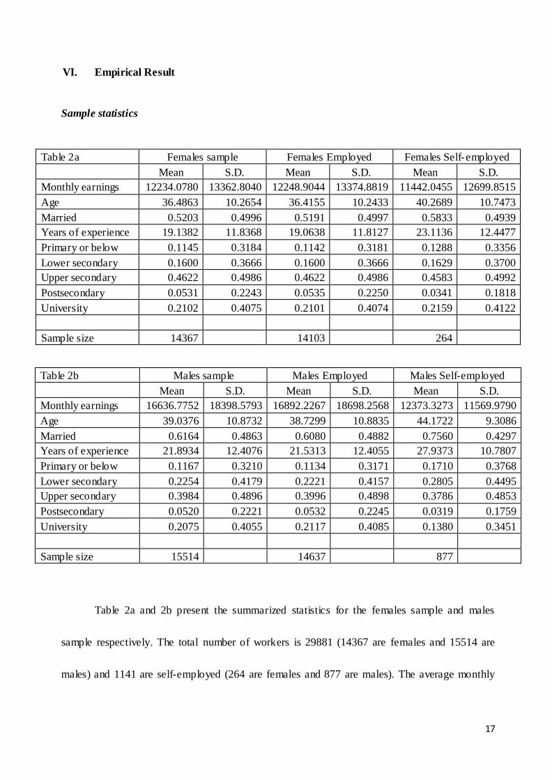
VI. Empirical Result

Sample statistics

Table 2a Females sample Females Employed Females Self-employed

Mean S.D. Mean S.D. Mean S.D.

Monthly earnings 12234.0780 13362.8040 12248.9044 13374.8819 11442.0455 12699.8515

Age 36.4863 10.2654 36.4155 10.2433 40.2689 10.7473

Married 0.5203 0.4996 0.5191 0.4997 0.5833 0.4939

Years of experience 19.1382 11.8368 19.0638 11.8127 23.1136 12.4477

Primary or below 0.1145 0.3184 0.1142 0.3181 0.1288 0.3356

Lower secondary 0.1600 0.3666 0.1600 0.3666 0.1629 0.3700

Upper secondary 0.4622 0.4986 0.4622 0.4986 0.4583 0.4992

Postsecondary 0.0531 0.2243 0.0535 0.2250 0.0341 0.1818

University 0.2102 0.4075 0.2101 0.4074 0.2159 0.4122

Sample size 14367 14103 264

Table 2b Males sample Males Employed Males Self-employed

Mean S.D. Mean S.D. Mean S.D.

Monthly earnings 16636.7752 18398.5793 16892.2267 18698.2568 12373.3273 11569.9790

Age 39.0376 10.8732 38.7299 10.8835 44.1722 9.3086

Married 0.6164 0.4863 0.6080 0.4882 0.7560 0.4297

Years of experience 21.8934 12.4076 21.5313 12.4055 27.9373 10.7807

Primary or below 0.1167 0.3210 0.1134 0.3171 0.1710 0.3768

Lower secondary 0.2254 0.4179 0.2221 0.4157 0.2805 0.4495

Upper secondary 0.3984 0.4896 0.3996 0.4898 0.3786 0.4853

Postsecondary 0.0520 0.2221 0.0532 0.2245 0.0319 0.1759

University 0.2075 0.4055 0.2117 0.4085 0.1380 0.3451

Sample size 15514 14637 877

Table 2a and 2b present the summarized statistics for the females sample and males

sample respectively. The total number of workers is 29881 (14367 are females and 15514 are

males) and 1141 are self-employed (264 are females and 877 are males). The average monthly

18

earnings of females is 12234 dollars and that of males is 16637 dollars. The two tables show that

the average monthly earnings of males is greater than that of females in the employed samples as

well as the self-employed samples. The average year of experience is 19 years for females and

22 years for males. There are a greater average number of years of experience for males than

females. The average age of the female respondents is 36 and that of male respondents is 39.

And 52% of the female respondents are married and 62% of male respondents are married. The

average age of respondents for males is older than that of females and more males is married

than that of females.

The percentages of female individuals with highest education levels attended are 11.5%,

16%, 46%, 5.3% and 21% for primary level or lower, lower secondary level, upper secondary

level, postsecondary level and university level or above respectively. These percentages of male

individuals are 11.7%, 22.5%, 39.8%, 5.2% and 20.8%. It is important to notice that there is a

higher percentage of females (72.6%) than males (65.8%) attended upper secondary or above

education level. Average monthly earnings of the employed are higher than the self-employed,

and the mean age for employed is younger than the self-employed for both females and males.

For the employed of both female sample and male sample 72.6% females and 66.45% males

with highest education levels attended for upper secondary or above level higher than that of

70.8% females and 54.9% males for the self-employed.

19

Riley (1979) mentioned that if education level is used as a signal for screening, it is

reasonable to believe that it should be an efficient signal. From Table 2a, we can see that the

percentage of presumed screened to obtain higher education level, namely upper secondary level,

postsecondary level and university level or above, is greater than these percentage of the

presumed unscreened. The screened jobs may require higher education (may be overly higher)

and individual who are choosing to be unscreened self-employed may have less education level

as they need not to “signal” themselves. So the higher education level of the screened jobs

supports the screening hypothesis.

As the employed have to be screened, their earnings are expected to be corrected

eventually overtime and hence their earnings would spread wider than the unscreened. In Table

2a and 2b the standard deviation of the employed are greater than the standard deviation of the

self-employed.

The employed generally obtain higher education level to “signal” themselves. Moreover,

the employed has a wider spread of earnings distribution when compare to self-employed. The

sample statistics consist with Riley’s mind as if the “signal” exists.

20

Chow test

In order to test whether earnings functions for males and females are different or not in

this project, Chow test is introduced to test whether the two earnings functions are equivalent.

For the employed sample:

F = 239.6412

Fc = 2.02

F > Fc

As F > Fc, we should reject the null hypothesis that the earnings functions of males and

females for the employed samples are equivalent.

For the self-employed sample:

F= 2.6497

Fc = 2.02

F > Fc

As F > Fc, we should reject the null hypothesis that the earnings functions of males and

females for the self-employed samples are equivalent.

For females and males, either the employed or the self-employed, should be estimated

separately as the Chow test concludes they are not equivalent.

21

Result of probit regression

Table 3a Marginal effect for dummy variable is P(Self)|1 – P(Self)|0 for females

Variables Coefficient Standard Error

Constant -0.0982* 0.0053

MT7 0.0120* 0.0021

A40 0.0493* 0.0062

OSE 0.0070* 0.0021

HKB -0.0014 0.0022

* means the coefficient of variable is statistically significant at 1% level

Table 3b Marginal effect for dummy variable is P(Self)|1 – P(Self)|0 for males

Variables Coefficient Standard Error

Constant -0.2224* 0.0148

MT7 0.0316* 0.0049

A40 0.1273* 0.0068

OSE 0.0310* 0.0032

HKB -0.0147* 0.0038

* means the coefficient of variable is statistically significant at 1% level

The results of probit regression are presented in Table 3a for females and Table 3b for

males. The results show that except the coefficient of females who born in Hong Kong all

variables are statistically significant at 1% level. It can be concluded that if the females

individual residence in Hong Kong for 7 years or more, age equal to or greater than 40, and is in

specific occupations mentioned before, she would be 1.2%, 4.9%, and 0.7% more likely to be

self-employed respectively. And if the male individuals residence in Hong Kong for 7 years or

more, age equal to or greater than 40, is in specific occupations mentioned before, and is not

born in Hong Kong he would be 3.1%, 12.7%, 3.1% and 1.5% more likely to be self-employed

respectively.

22

The expected Zi of the individuals can be calculated after obtaining the coefficients above.

Then the λ(Zi) can also be obtained by inverse Mills ratio, which is:

λ(Zi) = ф(Zi)/[1 - Φ(Zi)]

where ф is the standard normal density function and Φ is the standard normal cumulative

distribution function.

23

Result of Mincerian earnings equation (Mincer, 1974)

The result of sample selected earnings regressions is shown on Table 4. λ is introduced as

a variable to control for selection bias.

Table 4. Sample selected earnings regressions by gender

Females Males

Variables Employed Self-employed Employed Self-employed

Constant 7.7442* 8.5301* 7.9944* 8.6407*

(0.0268) (0.4670) (0.0243) (0.1952)

Married 0.0323# -0.1036 0.1984* 0.1158^ (0.0129) (0.1126) (0.0133) (0.0596)

Years of experience 0.0588* 0.0640* 0.0748* 0.0364*

(0.0019) (0.0157) (0.0017) (0.0093)

Years of experience squared -0.0010* -0.0012* -0.0013* -0.0007* (0.0000) (0.0003) (0.0000) (0.0002)

Lower secondary 0.0843* 0.1405 0.0944* 0.0201

(0.0233) (0.2026) (0.0199) (0.0733)

Upper secondary 0.5556* 0.2871 0.4405* 0.1284^ (0.0222) (0.2040) (0.0201) (0.0760)

Postsecondary 0.9762* 0.4711 0.7993* 0.1411

(0.0326) (0.3193) (0.0291) (0.1421)

University 1.3675* 0.6904* 1.2636* 0.5303* (0.0253) (0.2298) (0.0228) (0.0958)

Λ -2.2206* -0.1829 0.1735 * -0.0211

(0.1678) 0.1515) (0.5660) (0.0588) Adjusted R-squared 0.3001 (0.1043 0.3830 0.0836

Sample size 14103 264 14637 877

* means the coefficient of variable is statistically significant at 1% level

# means the coefficient of variable is statistically significant at 5% level

^ means the coefficient of variable is statistically significant at 10% level

24

The result shows that the return to experience of both employed and self-employed

groups for both males and females increase at a decreasing rate. One may also find that for males,

marriage would increase the earning of both employed and self-employed. However, marriage

shows less significant effect on females. The variables of years of experience are significantly

positive. In detail, for employed the return of experience for males is greater than that of females.

In contra, the return of experience for females is greater than that of males in the self-employed

sector.

From the result we can see that the higher the education level, the higher the earnings for

both samples. As the human capital theory suggests that education enhance productivity of the

individuals and hence the monthly earnings. The result supports the human capital theory as

education increase earnings of both samples, especially the self-employed sample as it is

presumed not affected by signaling effect.

However, the return of education levels increase more in the employed for both genders

than the self-employed which in the line of signaling does has positive effect on earnings. (Riley,

1979 and Chatterji, Seaman and Singell, 2003)

25

We can also see that the higher education the less increase in additional return for self-

employed than that of employed such as university or above level for the females, the additional

return is 137% for employed but only 69% for the self-employed which is only about a half of

the return of earnings to education of the employed. For the employed of both genders, achieving

higher education level brings much greater returns of education than the self-employed which is

supporting the screening hypothesis as education as a signal does gain positive return to earnings.

Therefore, although education does enhance productivity of individuals, using education as a

signal does exist in Hong Kong. (Heywood & Wei, 2004).

When comparing the effect of education level to earnings of different genders. Only the

return to education of lower secondary for employed males is greater than that of employed

females. For higher education levels, namely upper secondary, postsecondary, university or

above levels, females clearly earn higher return on it. This implies that females earn a greater

productivity from education than males do. Besides, females may need a stronger signal and earn

a greater portion of their return to education from using it as a signal. However, the stronger

signal needed by females does not means they are in disadvantageous in labor-market. It may be

a result of gender-differences of job natures (Chatterji, Seaman and Singell, 2003).

26

VII. Limitations

Firstly, this paper uses Hong Kong 2006 By-census 1% sample dataset which the full

sample contains 31022 individuals. However, the sample statistics show that only 1141

individuals are self-employed. The sample is small that makes many coefficient less significant

especially for the females self-employed sample which only include 264 individuals. Therefore,

if a larger sample such as 5% sample dataset can be used the result would be more representative.

Secondly, because of the limitations of the data, some characteristics and talents of the

individuals that may influence the education level as well as the earnings functions of the

individuals such as intelligence quotient have not been measured. Therefore, it is less able to

investigate whether education is used as a filter to screen out the less talented and eventually be

used by employers as a signal or education actually better equips and improves the productivity

of individual with same level of talent.

Thirdly, the variables used in the probit regression, which is used to capture the

characteristics of self-employed, are not perfect as mentioned before. However it is an alternative

because they do not alter the earning function. As a result the λ includes in the earnings functions

may not significant, but it is actually introduced as a variable to control for selection bias.

27

Lastly, this paper suggests although the signal does exists, education still enhance

productivity of an individual. Therefore, as education enhance productivity as well as generate

the private “signal”, it is not able to sure whether the public investments on education of

individuals generates greater social benefits than the social cost or not in this paper and more

work should be done by comparing the total social costs versus social benefits in order to

determine: “Is it worth us to invest so heavy on education or invest in the rest that could generate

more economic returns?”

28

VIII. Conclusion

In this project, Mincerian earning function is used for compare the education level to

earnings of both employed and self-employed by different genders. The Chow test is used to

provide evident that earnings functions of females and males is not equivalent which should be

estimated separately. The Heckman two-step procedure is used, in order to correct the selection

bias of the earnings functions. The result of probit regression states that individual reside in

Hong Kong for 7 years or more, age equal or greater than 40, and is small business manager, life

science and health professionals, salespersons and models or drivers and mob ile machine

operators would be more likely to be self-employed for both genders and if a male who is not

born in Hong Kong also would be more likely to be self-employed.

The result of the earnings functions show that higher education level would result in higher

monthly earnings either for the employed or the self-employed. It can be evident of human

capital theory that education enhances productivity of an individual. However, it is only part of

the picture. Another part of the picture supports the screening hypothesis by consist with the

thought of Riley (1979) as following:

Firstly, the sample statistics shows that the employed group which is presumed screened

has generally higher education level than that of the self-employed group which is presumed

29

unscreened. That means the screened jobs require higher education level, and people who choose

to be self-employed generally achieve lower education levels as the screened jobs require

individuals to signal themselves but individuals choose to be self-employed need not to do so.

Secondly, the employed has wider spread over than the self-employed in the earnings

distribution as the result of earnings correcting. It supports the screening hypothesis as the

employed have to be screened and their earnings are expected to be corrected eventually.

Thirdly, the additional return for self-employed for an additional education level achieved

generate less and less return eventually when comparing to those employed which implies

achieving higher education level generate greater and greater return for those who are employed

rather than those who are self-employed.

Besides, the result of this paper indicates that females generally attend higher education

level than that of males. And the return to education of females is greater than that of males

either the employed or the self-employed. From the self-employed, we can conclude that females

gain more productivity in education. Moreover, from the employed, the education levels for

females are used as a signal more intensively than that of males (Chatterji, Seaman and Singell,

2003).

30

All in all, this paper provides supports that use education level as signal does exists in

Hong Kong labor market. Employees may use it to signaling themselves and employers also rely

on it as a reference to determine the productivity of an employee or a potential employee.

However, the screening hypothesis does not explain everything of the earnings functions as the

positive return of education level to earnings for the self-employed. The rest of explanations of

the functions come to the human capital theory that education actually raises ones’ productivity.

And when comparing the return to education by genders, females gain more return on education

by both productivity and use it as a signal.

Reference

Addison, J.T. & Siebert W. S. (1997). Labour Markets in Europe: Issues of Harmonization and

Regulation. London: Dryden Press.

Becker, G. S. (1993). Human Capital (3rd ed.). Chicago and London: The University of Chicago

Press.

Chiswick, B. R. (1973). Schooling, Screening and Income. In Taubman, P. J. & Solmon, L.C.

(Eds.), Does College Matter? (pp. 151-158.). New York: Academic Press.

Chatterji, M., Seaman, P.T. & Singell, L.D. (2003). A test of signaling hypothesis. Oxford

Economic Papers, 55, pp.191-215

De Wit, G. & Van Winden, F. (1989) An empricial analysis of self-employment in Netrherlands,

Small Business Economics, 1, pp. 263-272

Denison, E. F. (1985). Trends in American economic growth. Washington, D.C.: Brookings

Institution.

Groot, W. & Oosterbeek, H. (1994) Earnings Effects of Different Components of Schooling;

Human Capital versus Screening. The Review of Economics and Statistics, 76(2),

pp. 317-321.

Gullason, E.T. (1998). A Test Of The Validity Of The Screening Hypothesis Versus The Human

Capital Theory Using The Wu-Hausman Specification Test For Endogeneity. The

Journal of Applied Business Research, 14 (3), pp.13-20.

Heckman, J.J. (1979). Sample selection bias as a specification error. Econometrica, 47(1), pp

153-171.

Heywood, J. S. & Wei, X. (2004). Education and Signaling: Evidence from a Highly

Competitive Labor Market. Education Economics, 12, pp. 1-16.

Layard, R. & Psacharopoulos, G. (1974). The Screening Hypothesis and the Returns to

Education. Journal of Political Economy, 82, pp. 985-998.

Mincer, J. (1974). Schooling, Experience, and Earning. New York: Columbia University Press.

Miller, P. W. & Volker P. (1984). The Screening Hypothesis: An application of The Wiles Test.

Economic Inquiry, 20, pp.72-83.

Riley, J. G. (1979). Testing the Educational Screening Hypothesis. Journal of Political Economy,

87, pp. 227-251.

Tao, H.-L. (2006). The Demand for Higher Education and a Test of the Extreme Screening

Hypothesis. Education Economics, 14(1), pp.75-88.

Thurow, L. (1975). Generating Inequality. New York: Basic Books.

Wolpin, K. (1977). Education and Screening. American Economic Review, 67, pp. 949-958