education, income and happiness: panel evidence for the uk

Empirical Economics (2020) 58:2573–2592https://doi.org/10.1007/s00181-018-1586-5

Education, income and happiness: panel evidencefor the UK

Felix R. FitzRoy1 ·Michael A. Nolan2

Received: 11 January 2018 / Accepted: 30 October 2018 / Published online: 14 November 2018© The Author(s) 2018

AbstractUsing panel data from theBHPSand itsUnderstandingSociety extension,we study lifesatisfaction (LS) and income over nearly two decades, for samples split by education,and age, to our knowledge for the first time. The highly educated went from lowest tohighest LS, though their average income was always higher. In spite of rapid incomegrowth up to 2008/2009, the less educated showed no rise in LS, while highly educatedLS rose after the crash despite declining real income. In panel LS regressions withindividual fixed effects, none of the income variables was significant for the highlyeducated.

Keywords Education · Income · Economic growth · Life satisfaction · Easterlinparadox

JEL Classification I31 · O47

1 Introduction

Education is correlated with both income and health—each of which, in turn, has apositive effect on life satisfaction (LS). Those with higher education generally haveaccess to more interesting and better-paid jobs, together with other non-pecuniarybenefits. Meanwhile, manual labour is systematically correlated with lower LS—soit is not surprising that (higher) education is generally considered to be beneficial forsubjective well-being, happiness or LS, as well as for objective individual economic

Electronic supplementary material The online version of this article (https://doi.org/10.1007/s00181-018-1586-5) contains supplementary material, which is available to authorized users.

B Michael A. [email protected]

1 School of Economics and Finance, University of St Andrews, St Andrews KY16 8QX, UK

2 Faculty of Business, Law and Politics, University of Hull, Hull HU6 7RX, UK

123

http://crossmark.crossref.org/dialog/?doi=10.1007/s00181-018-1586-5&domain=pdf

https://doi.org/10.1007/s00181-018-1586-5

2574 F. R. FitzRoy, M. A. Nolan

and social goals. Thus, in their wide-ranging, cross-country survey of ‘Happiness atWork’ based on Gallup World Poll data, De Neve and Ward (2017) find a highlysignificant, positive effect of high education on LS in the presence of many otherrelevant controls such as health, income and employment—although a gender splitfor a much smaller sample based on European Social Survey data then indicates thata similar effect is only evident for men.

It is, therefore, initially rather surprising that a previous study of LS with BritishHousehold Panel Survey (BHPS) data found negative or insignificant effects of highereducation in various specifications with numerous controls, while the positive effectwas robust in German SOEP data (FitzRoy et al. 2014). However, using only Wave 1BHPS data, Clark and Oswald (1996) report a negative relationship between a morespecific job satisfaction variable and both education and comparison income. Viaanalysis of Wave 6–14 of the BHPS data, Powdthavee (2010) shows mainly negativeestimates for education controls in pooled OLS estimation of LS and insignificantestimates for fixed-effects estimation. Green (2011) finds a negative effect of highereducation on LSwith Australian (HILDA) data using many controls, but Nikolaev andRusakov (2016) find that higher education has a positive and increasing effect on LSfrom about the age of 35 in the same data set. Nikolaev (2016) also reports generallypositive associations of education with various components of LS with the same data.Adding to conflicting results from HILDA, Powdthavee et al. (2015) estimate a struc-tural model of education and life satisfaction and conclude that the direct effect ofeducation is negative, while positive associations arise from the well-known positiveeffects of education on income and health. Overall, the existing literature containsmixed findings.

Here, we consider the UK over a rather longer time series. We extend the BHPSpanel with the corresponding component of the Understanding Society data set (partof which involves individuals drawn from the BHPS) to study the development of lifesatisfaction (LS) and income across a couple of decades, in different education (andage) groups. Real household income (deflated by the Consumer Prices Index1) wasalways highest for the highly educated and for all groups grew substantially in the10 years up to the financial crash of 2008/2009. The subsequent decline and partialrecovery were steepest for the highly educated. That group also saw a rise in averagehousehold size around the time of the crash, whereas the households of the leasteducated tended to become smaller.

LS, on the other hand, rose fastest for the highly educated from a surprising lowestto being highest among the education groups, a significant increase over a periodwhen the proportion of highly educated roughly doubled. LS declined steeply forthe low education group up to and beyond the crash, in spite of their rising income.Overall, average LS declined pre-crash despite rapid income growth. Except for thehighly educated before the crash, whose income and LS both increased, these resultscontradict standard economic growth theories, but are consistent with the Easterlinparadox found in macro data. Of course, mainly negative correlations of averages areno guarantee of the sign of the average of LS–income correlations at the individual

1 Measured by ONS series D7BT.

123

Education, income and happiness: panel evidence for the UK 2575

level—in general terms, this point can be traced back at least to Robinson (1950), andthe coining of the term ‘ecological fallacy’ in Selvin (1958).

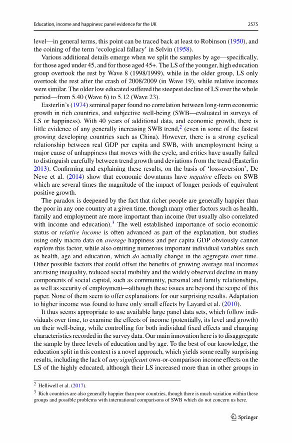
Various additional details emerge when we split the samples by age—specifically,for those aged under 45, and for those aged 45+. The LS of the younger, high educationgroup overtook the rest by Wave 8 (1998/1999), while in the older group, LS onlyovertook the rest after the crash of 2008/2009 (in Wave 19), while relative incomeswere similar. The older low educated suffered the steepest decline of LS over thewholeperiod—from 5.40 (Wave 6) to 5.12 (Wave 23).

Easterlin’s (1974) seminal paper found no correlation between long-term economicgrowth in rich countries, and subjective well-being (SWB—evaluated in surveys ofLS or happiness). With 40 years of additional data, and economic growth, there islittle evidence of any generally increasing SWB trend,2 (even in some of the fastestgrowing developing countries such as China). However, there is a strong cyclicalrelationship between real GDP per capita and SWB, with unemployment being amajor cause of unhappiness that moves with the cycle, and critics have usually failedto distinguish carefully between trend growth and deviations from the trend (Easterlin2013). Confirming and explaining these results, on the basis of ‘loss-aversion’, DeNeve et al. (2014) show that economic downturns have negative effects on SWBwhich are several times the magnitude of the impact of longer periods of equivalentpositive growth.

The paradox is deepened by the fact that richer people are generally happier thanthe poor in any one country at a given time, though many other factors such as health,family and employment are more important than income (but usually also correlatedwith income and education).3 The well-established importance of socio-economicstatus or relative income is often advanced as part of the explanation, but studiesusing only macro data on average happiness and per capita GDP obviously cannotexplore this factor, while also omitting numerous important individual variables suchas health, age and education, which do actually change in the aggregate over time.Other possible factors that could offset the benefits of growing average real incomesare rising inequality, reduced social mobility and the widely observed decline in manycomponents of social capital, such as community, personal and family relationships,as well as security of employment—although these issues are beyond the scope of thispaper. None of them seem to offer explanations for our surprising results. Adaptationto higher income was found to have only small effects by Layard et al. (2010).

It thus seems appropriate to use available large panel data sets, which follow indi-viduals over time, to examine the effects of income (potentially, its level and growth)on their well-being, while controlling for both individual fixed effects and changingcharacteristics recorded in the survey data. Ourmain innovation here is to disaggregatethe sample by three levels of education and by age. To the best of our knowledge, theeducation split in this context is a novel approach, which yields some really surprisingresults, including the lack of any significant own-or-comparison income effects on theLS of the highly educated, although their LS increased more than in other groups in

2 Helliwell et al. (2017).3 Rich countries are also generally happier than poor countries, though there is much variation within thesegroups and possible problems with international comparisons of SWB which do not concern us here.

123


the period. Another puzzle is why the high education group had lowest LS initially,but overtook the less educated to become most satisfied while higher education wasrapidly expanding—see Blundell et al. (2016).

2 Data andmethodology

Our main data are taken from Waves 6–10 and 12–18 of the British Household PanelSurvey4 (BHPS), covering a period that runs from1996/1997 to 2008/2009 (Universityof Essex, Institute for Social and Economic Research 2010) and from those partsof Waves 2–6 of the section of the new Understanding Society5 longitudinal study(Kantar Public, NatCen Social Research, University of Essex. Institute for Social andEconomic Research 2016) that relate to active, consenting former members of theBHPS sample, covering a period6 from 2010–2011 to 2014–2015. An initial baselineof 214,704 observations is available, across the full income range. However, as isevident in Fig. 1, LS data were not collected for BHPSWave 11 (17,609 observationsfor 2001/2002). Also evident from Fig. 1 (and its 95% confidence limits) is the fact thatnot all of the time variation in average LS can be attributed to sampling variation. Forregression analysis, we generate results for up to 178,382 observations across 23,748individuals, with those cases where there are missing values, and the highest incomeoutliers,7 excluded. As usual, we note the deliberate over-sampling of the smallernations of the UK since Wave 9—so that about half of the individuals in the BHPSare from Scotland, Wales and Northern Ireland,8 compared with less than 20% in theoverall population.

A plausible hypothesis is that those with higher education, who generally havethe best-paid and most interesting jobs, would be most likely to enjoy increasing lifesatisfaction with higher incomes, so we split the sample into three groups. For theinitial BHPS waves, classification through the International Standard Classificationof Education (ISCED) is available—and the split is into higher (ISCED categories5a and 6—for first degrees and higher degrees), middle (ISCED categories 3a and5b—for higher secondary and middle/higher vocational) and low (ISCED categoriesprimary, low secondary and 3c—low secondary vocational) education. However, no

4 The earlier waves of the BHPS (up to Wave 10) were limited in coverage to Great Britain. The full UK(including Northern Ireland) is covered in Waves 12–18. BHPS data are available via the UK Data Service(formerly the UK Data Archive).5 Since Wave 2 of Understanding Society is the first to follow on from BHPS Wave 18, we re-number theUnderstanding Society Waves (2–6) as 19–23.6 With interviews taking place across calendar year boundaries (and two boundaries for Waves 21–22),a given Wave will see certain regressors defined according the year of interview, as appropriate to eachindividual.7 A cut-off of 9.5 for the natural logarithm of (deflated) monthly household income is around £160,000 peryear. This reduces the number of observations by 684, whilst a further 19 cases are excluded due to issuesrelating to the identification of individuals across waves. By definition, regressors measuring changes inhousehold income between successive waves are not available for the first wave in which any individualresponds. This is some 18,010 observations.8 Across Waves 6–23, 44% of observations are for individuals outside England. Northern Ireland was notincluded in the BHPS data until Wave 11 (2001/2002).

123


Fig. 1 Life satisfaction, BHPS and Understanding Society (USoc), Waves 6–10, 12–23

ISCED codings are yet available for the Understanding Society waves—so that thethree-way split had to be undertaken on the basis of a less sophisticated derived highestqualification variable.9 Since the crucial difference is the striking and quite counter-intuitive contrast between the higher and the two lower groups, we aggregate thelatter pair to simplify Figs. 2, 3 and 4 (again, including confidence intervals) and ourregressions.

Our estimation approach is quite similar to FitzRoy et al. (2014)—we use individualfixed effects in estimation of a LS equation with quite a number of controls—manyof which are fairly standard when using BHPS data. These include marital status(including cohabiting), number of children, health status, education, labour marketstatus, time spent in panel, whether year of last interview, log household size, age(via six age dummies to create seven age categories), housing ownership status, wavenumber and regions. We also tested the alternative of a traditional polynomial agespecification—and found results quite similar to FitzRoy et al. (2014).

InOnlineAppendix, samplemeans are shown formany of the controls in TableA1a:the sample is also split by education level (see Fig. 5 as well). We also followMoulton(1990) in recognising the potential (cluster related) effect of aggregate regressors onstandard errors. Given that we are focusing on the estimation of individual-specificfixed-effects regressions, we assume clustering at the level of the individual.

For the crucial test of the effects of income on LS in different education groups,we include (deflated) own household income (for the month before interview) andcomparison (peer group) income separately. The definition used here for comparisonincome follows that employed by FitzRoy et al. (2014)—whereby comparison groupsare defined by age bands (between 3 years younger and 6 years older), sex, education

9 This split is essentially between degrees, A levels and GCSEs (alongside others, and none).

123


Fig. 2 Life satisfaction by education, BHPS and USoc, Waves 6–10 and 12–23

Fig. 3 Life satisfaction by education, BHPS and USoc, aged <45, Waves 6–10 and 12–23

(two categories), region (three categories) and Wave. The groups are quite broad inspecification—with a median cell size around 335 members, and a bottom decile at 80members. We also experiment with the inclusion of upward and downward changes inownhousehold income, allowing for asymmetricLS responses. In addition to includinga full set of regional dummies (with Greater London as the reference region), we

123


Fig. 4 Life satisfaction by education, BHPS and USoc, aged 45+, Waves 6–10 and 12–23

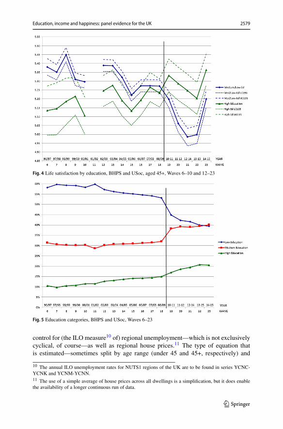
Fig. 5 Education categories, BHPS and USoc, Waves 6–23

control for (the ILO measure10 of) regional unemployment—which is not exclusivelycyclical, of course—as well as regional house prices.11 The type of equation thatis estimated—sometimes split by age range (under 45 and 45+, respectively) and

10 The annual ILO unemployment rates for NUTS1 regions of the UK are to be found in series YCNC-YCNK and YCNM-YCNN.11 The use of a simple average of house prices across all dwellings is a simplification, but it does enablethe availability of a longer continuous run of data.

123


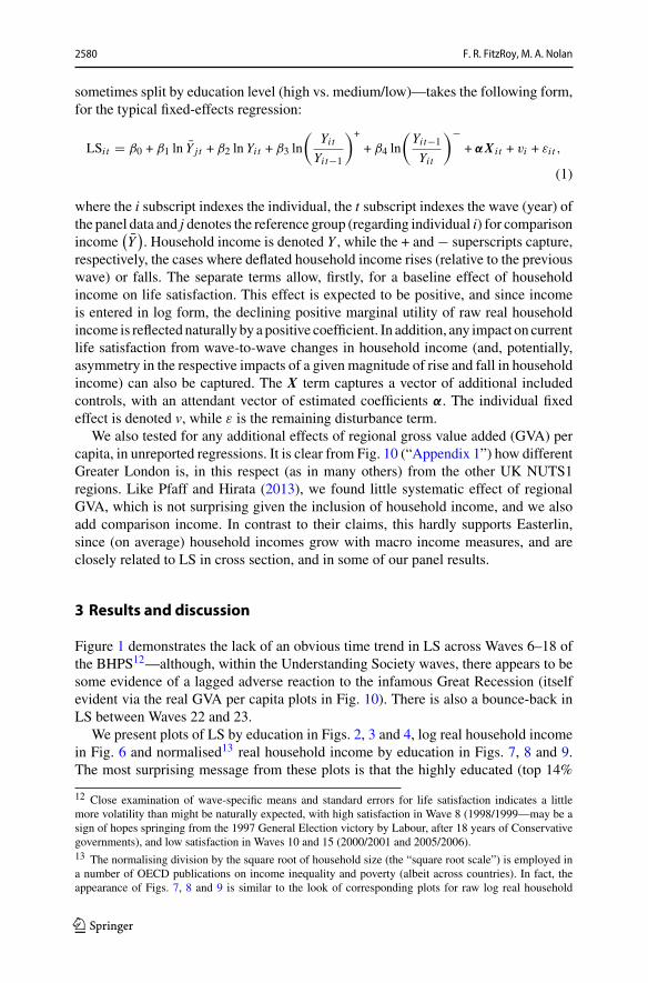
sometimes split by education level (high vs. medium/low)—takes the following form,for the typical fixed-effects regression:

LSi t � β0 + β1 ln Y j t + β2 ln Yit + β3 ln

(YitYit−1

)+

+ β4 ln

(Yit−1

Yit

)−+ αX i t + vi + εi t ,

(1)

where the i subscript indexes the individual, the t subscript indexes the wave (year) ofthe panel data and j denotes the reference group (regarding individual i) for comparisonincome

(Y

). Household income is denoted Y , while the + and − superscripts capture,

respectively, the cases where deflated household income rises (relative to the previouswave) or falls. The separate terms allow, firstly, for a baseline effect of householdincome on life satisfaction. This effect is expected to be positive, and since incomeis entered in log form, the declining positive marginal utility of raw real householdincome is reflected naturally by a positive coefficient. In addition, any impact on currentlife satisfaction from wave-to-wave changes in household income (and, potentially,asymmetry in the respective impacts of a given magnitude of rise and fall in householdincome) can also be captured. The X term captures a vector of additional includedcontrols, with an attendant vector of estimated coefficients α. The individual fixedeffect is denoted v, while ε is the remaining disturbance term.

We also tested for any additional effects of regional gross value added (GVA) percapita, in unreported regressions. It is clear from Fig. 10 (“Appendix 1”) how differentGreater London is, in this respect (as in many others) from the other UK NUTS1regions. Like Pfaff and Hirata (2013), we found little systematic effect of regionalGVA, which is not surprising given the inclusion of household income, and we alsoadd comparison income. In contrast to their claims, this hardly supports Easterlin,since (on average) household incomes grow with macro income measures, and areclosely related to LS in cross section, and in some of our panel results.

3 Results and discussion

Figure 1 demonstrates the lack of an obvious time trend in LS across Waves 6–18 ofthe BHPS12—although, within the Understanding Society waves, there appears to besome evidence of a lagged adverse reaction to the infamous Great Recession (itselfevident via the real GVA per capita plots in Fig. 10). There is also a bounce-back inLS between Waves 22 and 23.

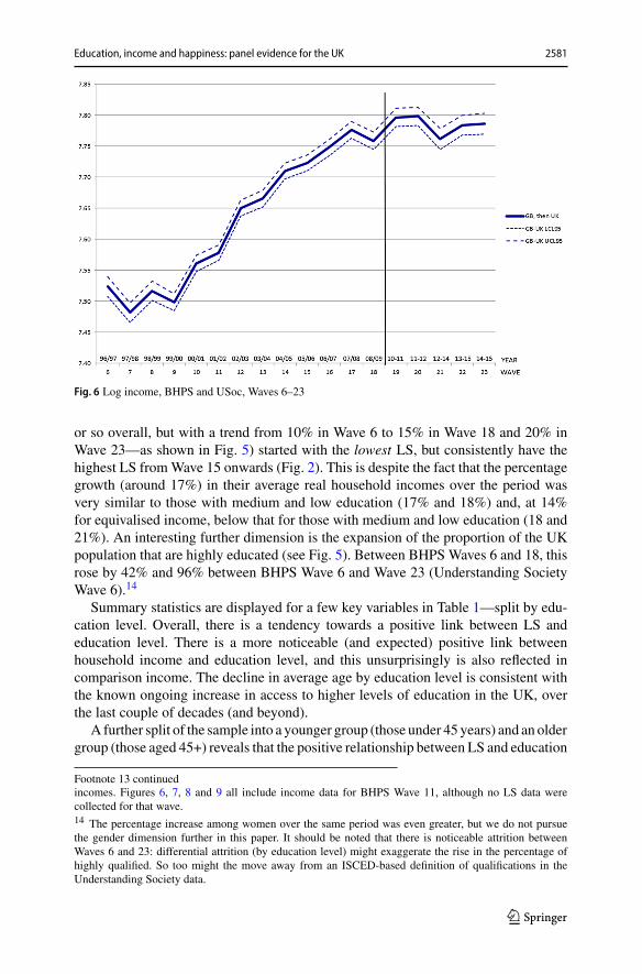
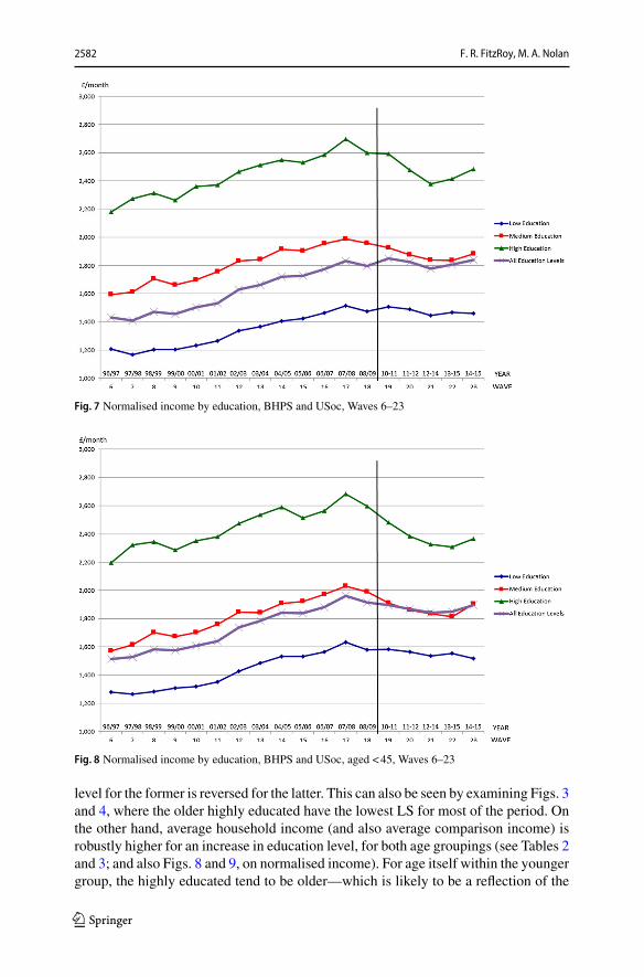
We present plots of LS by education in Figs. 2, 3 and 4, log real household incomein Fig. 6 and normalised13 real household income by education in Figs. 7, 8 and 9.The most surprising message from these plots is that the highly educated (top 14%

12 Close examination of wave-specific means and standard errors for life satisfaction indicates a littlemore volatility than might be naturally expected, with high satisfaction in Wave 8 (1998/1999—may be asign of hopes springing from the 1997 General Election victory by Labour, after 18 years of Conservativegovernments), and low satisfaction in Waves 10 and 15 (2000/2001 and 2005/2006).13 The normalising division by the square root of household size (the “square root scale”) is employed ina number of OECD publications on income inequality and poverty (albeit across countries). In fact, theappearance of Figs. 7, 8 and 9 is similar to the look of corresponding plots for raw log real household

123


Fig. 6 Log income, BHPS and USoc, Waves 6–23

or so overall, but with a trend from 10% in Wave 6 to 15% in Wave 18 and 20% inWave 23—as shown in Fig. 5) started with the lowest LS, but consistently have thehighest LS fromWave 15 onwards (Fig. 2). This is despite the fact that the percentagegrowth (around 17%) in their average real household incomes over the period wasvery similar to those with medium and low education (17% and 18%) and, at 14%for equivalised income, below that for those with medium and low education (18 and21%). An interesting further dimension is the expansion of the proportion of the UKpopulation that are highly educated (see Fig. 5). Between BHPS Waves 6 and 18, thisrose by 42% and 96% between BHPS Wave 6 and Wave 23 (Understanding SocietyWave 6).14

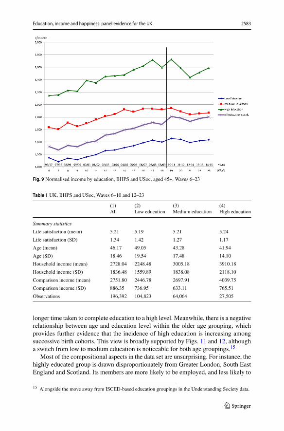
Summary statistics are displayed for a few key variables in Table 1—split by edu-cation level. Overall, there is a tendency towards a positive link between LS andeducation level. There is a more noticeable (and expected) positive link betweenhousehold income and education level, and this unsurprisingly is also reflected incomparison income. The decline in average age by education level is consistent withthe known ongoing increase in access to higher levels of education in the UK, overthe last couple of decades (and beyond).

A further split of the sample into a younger group (those under 45 years) and an oldergroup (those aged 45+) reveals that the positive relationship between LS and education

Footnote 13 continuedincomes. Figures 6, 7, 8 and 9 all include income data for BHPS Wave 11, although no LS data werecollected for that wave.14 The percentage increase among women over the same period was even greater, but we do not pursuethe gender dimension further in this paper. It should be noted that there is noticeable attrition betweenWaves 6 and 23: differential attrition (by education level) might exaggerate the rise in the percentage ofhighly qualified. So too might the move away from an ISCED-based definition of qualifications in theUnderstanding Society data.

123


Fig. 7 Normalised income by education, BHPS and USoc, Waves 6–23

Fig. 8 Normalised income by education, BHPS and USoc, aged <45, Waves 6–23

level for the former is reversed for the latter. This can also be seen by examining Figs. 3and 4, where the older highly educated have the lowest LS for most of the period. Onthe other hand, average household income (and also average comparison income) isrobustly higher for an increase in education level, for both age groupings (see Tables 2and 3; and also Figs. 8 and 9, on normalised income). For age itself within the youngergroup, the highly educated tend to be older—which is likely to be a reflection of the

123


Fig. 9 Normalised income by education, BHPS and USoc, aged 45+, Waves 6–23

Table 1 UK, BHPS and USoc, Waves 6–10 and 12–23

(1) (2) (3) (4)All Low education Medium education High education

Summary statistics

Life satisfaction (mean) 5.21 5.19 5.21 5.24

Life satisfaction (SD) 1.34 1.42 1.27 1.17

Age (mean) 46.17 49.05 43.28 41.94

Age (SD) 18.46 19.54 17.48 14.10

Household income (mean) 2728.04 2248.48 3005.18 3910.18

Household income (SD) 1836.48 1559.89 1838.08 2118.10

Comparison income (mean) 2751.80 2446.78 2697.91 4039.75

Comparison income (SD) 886.35 736.95 633.11 765.51

Observations 196,392 104,823 64,064 27,505

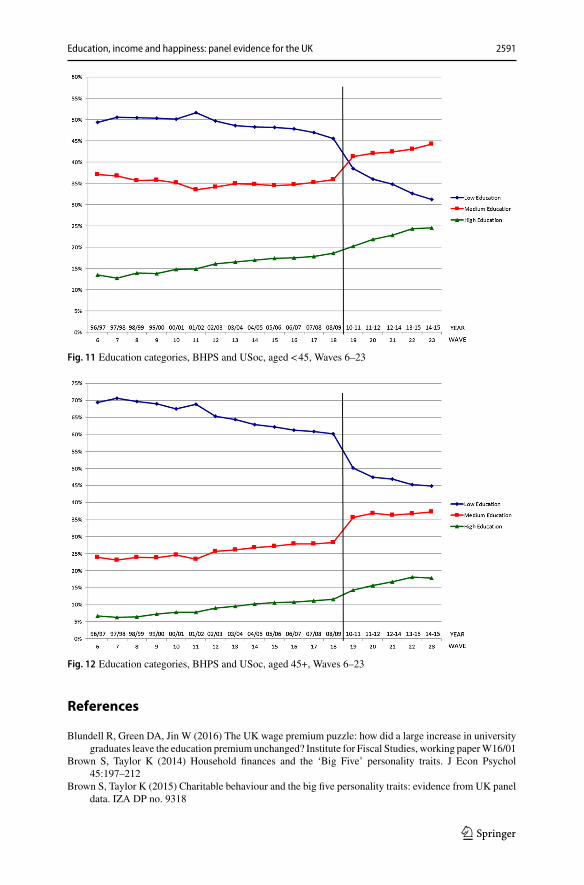
longer time taken to complete education to a high level. Meanwhile, there is a negativerelationship between age and education level within the older age grouping, whichprovides further evidence that the incidence of high education is increasing amongsuccessive birth cohorts. This view is broadly supported by Figs. 11 and 12, althougha switch from low to medium education is noticeable for both age groupings.15

Most of the compositional aspects in the data set are unsurprising. For instance, thehighly educated group is drawn disproportionately from Greater London, South EastEngland and Scotland. Its members are more likely to be employed, and less likely to

15 Alongside the move away from ISCED-based education groupings in the Understanding Society data.

123



(1) (2) (3) (4)Under 45 years Low education,

<45Mediumeducation, <45

High education,<45

Summary statistics



Age (mean) 30.68 30.22 30.35 32.64

Age (SD) 8.41 8.93 8.33 6.68





Observations 98,002 45,272 35,934 16,796


(1) (2) (3) (4)Aged 45+ Low education,

45+Mediumeducation, 45+

High education,45+

Summary statistics



Age (mean) 61.60 63.36 59.79 56.52

Age (SD) 11.54 11.71 10.99 9.61





Observations 98,390 59,551 28,130 10,709

be unemployed or to be long-term sick or disabled (across the full age range and onboth sides of the age split). They are also less likely to rent their dwelling. Among thoseaged 45+, the highly educated are less likely to be retired and they enjoy a markedhealth advantage (present, to a lesser extent, in the younger age range too). Perhaps lessobvious is the fact that the highly educated under 45 years have a lower average house-hold size than the low or medium educated (maybe due in part to later marriage andstarting of a family), but, among those aged 45+, the highly educated have the highestaverage household size—possibly linked to a lower proportion having been widowed.

Our first estimation results are in Table 4, containing estimates of LS fixed-effectsregressions across all education levels—initially across the entire age range, and thenfor younger (<45) and older (45+) subgroups. Controls for high education are included(among the long list of controls), with an interaction to allow for a differential impactof high education on LS from Wave 14 (2004/2005) onwards (in line with Fig. 2).

123


Table 4 Individual fixed effects, across education—UK, BHPS and USoc, Waves 6–10 and 12–23

Regressor All <45 45+

Comparison income (log form) −0.171*** 0.091 −0.307***

(−3.57) (1.07) (−4.80)

Household income (log form) 0.040*** 0.063*** 0.012

(4.30) (5.03) (0.91)

Household income upward change 0.023*** 0.024** 0.018

(3.14) (2.54) (1.64)

Household income downward change size −0.001 0.010 −0.011

(−0.07) (0.74) (−0.77)

Highly qualified * Wave 14+ (interaction) 0.113*** 0.106*** 0.127***

(6.03) (4.48) (3.96)

Observations 178,382 85,350 93,032

Individuals 23,748 14,745 12,643

Dependent variableLife satisfaction. Controls for marital status (including cohabiting), number of children,health status, education, labour market status, time in panel, year of last interview, household size, agegroupings, housing ownership, wave number and regions are included. Standard errors clustered at theindividual level, robust t-statistics in parentheses***p<0.01; **p<0.05; *p<0.1

We report only coefficients of the various income variables, plus those for the higheducation * Wave 14+ interaction. A positive interaction effect is indeed evident forWaves 14–23, but the overall effect of being highly educated across those waves issignificant at the 5% level only for the 45+ age range.16 Own income and its upwardchanges have strong positive effects for the whole sample, and for those under 45 yearstaken alone.Meanwhile, comparison incomehas the positive, signalling effect for themthat was found previously for those under 45 years17—but the effect is statisticallyinsignificant in our case. The usual negative effect for comparison income is againfound for those aged 45+, or for the whole sample across the entire age range. Itshould be noted that the number of individuals reported in the first column of Table 4,for the whole sample, cannot be expected to be the same as the sum of the totals inthe other two columns (for the age split). This is because the observations for someindividuals can be found on both sides of the age split boundary.

Although the alternative of pooled cross-sectional estimation is problematic for ourunbalanced panel data, we have included Table A2a inOnlineAppendix, for additionalcontext—with standard errors clustered this time by the comparison income groupingregressor. This shows similar comparison income results to those found previouslyin Table 8 of FitzRoy et al. (2014)—with a significant negative estimate for the full

16 Nikolaev and Rusakov (2016) find a positive effect of education on LS that increases with age inAustralian panel data.17 FitzRoy et al. (2014) put forward a ‘hare and tortoise’ model, as a plausible basis to explain a positiveeffect for comparison income amongst younger people (especially later developers, who can see higherincomes for their peers as a signal of the potential for their own future). Meanwhile, older people may tendto realise that they are unlikely to attain higher incomes of their peers—if they have already had many yearsof opportunity, with such incomes remaining unrealised.

123


age range and also for the 45+ sample. Estimates for own household income are alsobroadly in line with that earlier work.18 Moreover, unreported regressions across thewhole age range with comparison income interacted with the age grouping controlcategories and own income interacted with an ‘aged 45+’ dummy generated chieflysimilar results to those in Table 24 of FitzRoy et al. (2014), both for fixed-effects andfor pooled OLS.

In Table 5, we report the same specification for the highly educated, with the reallyremarkable result that none of the standard income variables is significant for eitherage group (or across the full age range). Recall, from Fig. 2, that wave-specific LSarithmetic means rose significantly between BHPS Wave 6 and BHPS Wave 18 forthe highly educated, while the number of highly educated individuals rose by 50%(Fig. 5). Figure 3 indicates an increase in LS for the younger age group among thehighly educated, but no significant change for the older age group. The impact of theGreat Recession did seem to push down LS somewhat across Waves 20–22, albeitwith a bounce-back in Wave 23. These trends in LS must be due to other factors.Of our controls, a few do have statistically significant attached estimates. For thefull age range, as expected, economic activity status categories such as employee,self-employed, retirement, family care and full-time education are all positive forLS, relative to unemployment, and long-term sickness or disability is negative. Beingmarried or cohabiting is positive for LS, comparedwith being single and nevermarried.Good health and bad health each have the expected impact on LS, compared withthe baseline health category. Sampling variation may be a component in explainingthe insignificance of income regressors (especially given that this education groupingcontains fewer observations). In an effort to investigate the importance of low statisticalpower for our findings, a similar fixed-effects regression specification was estimatedwith the log of real household income as the dependent variable. This generated quitea few more statistically significant estimates—and overall goodness of fit measuresaround 5–7 times greater. The pooled cross-sectional results for this group (Table A2b)do not appear to offer solutions to this puzzle: instead, alongside some standard positiveeffects for own household income level, some additional queries are raised—by thesignificant negative estimate for comparison income among those under 45 years, andalso the positive estimates for the magnitude of negative changes in own income.

For medium and low education (Table 6), the effect of comparison income onLS is almost fully consistent with FitzRoy et al. (2014)—although only statisticallysignificant at the 10% level (and still negative) for the younger age range. However,own income and upward changes are only positive and significant for those agedunder 45. For this stratum of education, the older group sees the only substantial pre-recession decline in LS (Fig. 4). Both age groups have rising (normalised) real income,pre-recession (Figs. 8 and 9). Table 6 shows a negative effect of comparison incomefor the 45+ group, and that—together with the rising real income trend—could be partof the explanation for a pre-recession fall in LS. The offsetting negative externalities ofeconomic growth, and associated social change such as increasing prevalence of non-standard and precarious employment, would instead be expected to impact especially

18 However, that earlier work did not have additional regressors for upward and downward changes in ownincome.

123


Table 5 Individual fixed effects, high education—UK, BHPS and USoc, Waves 6–10 and 12–23


Comparison income (log form) −0.038 −0.020 0.031

(−0.41) (−0.13) (0.25)

Household income (log form) 0.016 0.043 −0.022

(0.69) (1.53) (−0.60)

Household income upward change 0.016 0.008 0.031

(1.05) (0.46) (1.14)

Household income downward change size 0.010 0.048 −0.033

(0.38) (1.46) (−0.84)

Highly qualified * Wave 14+ (interaction) 0.028 −0.243 0.403

(0.18) (−1.12) (1.41)

Observations 25,514 15,228 10,286

Individuals 3,427 2686 1419

Dependent variable Life satisfaction. Controls as in Table 4, except for education***p <0.01; **p <0.05; *p <0.1

Table 6 Individual fixed effects, medium/low education—UK, BHPS and USoc, Waves 6–10 and 12–23


Comparison income (log form) −0.200*** 0.228* −0.362***

(−3.41) (1.93) (−4.90)

Household income (log form) 0.041*** 0.060*** 0.019

(4.02) (4.19) (1.30)

Household income upward change 0.025*** 0.031*** 0.014

(2.90) (2.66) (1.15)

Household income downward change size −0.006 −0.001 −0.009

(−0.51) (−0.04) (−0.59)

Observations 152,868 70,122 82,746

Individuals 21,390 13,015 11,307

Dependent variable Life satisfaction. Controls as in Table 4, except for education (medium dummy only)***p<0.01; **p<0.05; *p<0.1

on the younger less qualified persons.19 Corresponding pooled cross-sectional results(Table A2c) also appear similar to their counterparts for the full sample across thewhole education range—albeit now with a statistically significant positive effect ofcomparison income on LS, for those aged under 45.

Given especially our struggle to explain life satisfaction for the highly educated,we consider the potential for a role of the Big Five personality traits, and especiallyneuroticism—as examined by Proto and Rustichini (2015), and found to ‘mediate theeffect of income on life satisfaction’. The UK part of their work uses the BHPS data.

19 Unfortunately, such trends are not picked up by means of the standard labour market controls includedwithin our regression specifications.

123


However, one practical difficulty is that only BHPSWave 15 (2005/2006) includes BigFive data—as also used in the household finances context by Brown and Taylor (2014).Proto and Rustichini (2015) argue—quite plausibly—that such traits are very stablefor most people across much of their lifespan. However, fixed-effects estimation couldnot use rawBig Five scores taken from a singlewave.Much of the analysis in Proto andRustichini (2015) is based on the interaction between (standardised) Big Five scoresand a quadratic function of income, and they also include random-effects estimation.For our investigations, the assumed zero correlation between the disturbances and theregressors, inherent in random-effects estimation, appears to be a binding (and distort-ing) constraint. Also, since Understanding Society Wave 3 (Wave 20 within our com-posite panel, for 2012–2014) also includesBigFive data—asusedbyBrownandTaylor(2015) to examine charitable givingbehaviour—wealso incorporated that information.

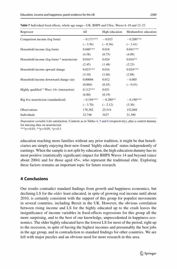
Although we standardise neuroticism scores prior to regression estimation, we donot undertake a preliminary regression to generate residuals as a replacement for thestandardised scores, to net out certain systematic effects. This is largely because Protoand Rustichini (2015) find little difference in the results on such a basis. Our resultsare given in Table 7—to compare with the respective left-hand columns of Tables 4,5 and 6. In each instance, estimates from previously listed regressors remain verysimilar. However, in two out of three instances, the income–neuroticism interaction’sestimates are statistically significant at the 5% level. Although it is for the highlyqualified that the estimate is insignificant, its similar magnitude at least suggests thepossibility that insignificance may be linked to the smaller sample size. Meanwhile,the neuroticism score estimates are significant and negative in all three columns ofTable 7. Overall, it seems that the income–personality trait interactionmay offer usefuladditional evidence, although it still appears that the picture is less clear for highlyeducated individuals than for others (see Online Appendix Tables A2di–A2diii forfull sets of regression results). Of course, this impression is emphasised by our (well-founded) primary concentration on fixed-effects estimation—rather than pooled OLSor random effects, both of which generate greater statistical significance for more ofthe included regressors.20 Note that our specifications including the Big Five have asystematic linkage with BHPS attrition—in the sense that any individual who left thepanel prior to Wave 15 (and had not returned by Wave 23) cannot have a score for anyof the Big Five personality traits.21

Thus, in one sense we disagree with Easterlin (2013) by finding rising householdincomes and LS for the high education group up to the recession, but we are consis-tent with his paradox for the less (low/medium) educated—since LS declined over thisperiod in spite of faster rising income. Our fixed-effects estimation highlights a majorpuzzle—the almost complete lack of significance of any of the income variables inexplaining rising LS for the high education sample. With the expansion of UK higher

20 Indeed, unreported results for specifications to measure “between” effects—essentially using the indi-vidual’s across-time mean of each variable to focus on cross-sectional variation—demonstrate statisticallysignificant coefficients for logged own income, and almost always also its interaction with neuroticism, forthe various groupings in Tables 4, 5 and 6.21 A (neuroticism) missing value dummy was included, as a control. Its attached estimate was negativebut insignificant under fixed-effects estimation—and of the same sign and greater significance for randomeffects, and for pooled OLS estimation of the highly educated sub-sample.

123


Table 7 Individual fixed effects, whole age range—UK, BHPS and USoc, Waves 6–10 and 12–23

Regressor All High education Medium/low education

Comparison income (log form) −0.171*** −0.033 −0.200***

(−3.56) (−0.36) (−3.41)

Household income (log form) 0.040*** 0.018 0.041***

(4.38) (0.75) (4.09)

Household income (log form) * neuroticism 0.016** 0.024 0.016**

(2.45) (1.48) (2.23)

Household income upward change 0.023*** 0.016 0.024***

(3.10) (1.04) (2.88)

Household income downward change size 0.00004 0.012 −0.005

(0.004) (0.45) (−0.43)

Highly qualified * Wave 14+ (interaction) 0.112*** 0.031

(6.00) (0.19)

Big five neuroticism (standardised) −0.194*** −0.280** −0.190***

(−3.70) (−2.12) (3.30)

Observations 178,382 25,514 152,868

Individuals 23,748 3427 21,390

Dependent variable Life satisfaction. Controls as in Tables 4, 5 and 6 (respectively), plus a control dummyfor missing data on neuroticism***p<0.01; **p<0.05; *p<0.1

education reaching more families without any prior tradition, it might be that benefi-ciaries are simply enjoying their new-found ‘highly educated’ status independently ofearnings. When the sample is not split by education, the high education dummy has itsmost positive (statistically significant) impact for BHPS Waves 14 and beyond (sinceabout 2004) and for those aged 45+, who represent the traditional elite. Exploringthese factors remains an important topic for future research.

4 Conclusions

Our results contradict standard findings from growth and happiness economics, butdeclining LS for the older least educated, in spite of growing real income until about2010, is certainly consistent with the support of this group for populist movementsin several countries, including Brexit in the UK. However, the obvious correlationbetween rising income and LS for the highly educated up to the crash leaves theinsignificance of income variables in fixed-effects regressions for this group all themore surprising, and to the best of our knowledge, unprecedented in happiness eco-nomics. The older highly educated have the lowest LS for most of the period, right upto the recession, in spite of having the highest incomes and presumably the best jobsin the age group, and in contradiction to standard findings for other countries. We areleft with major puzzles and an obvious need for more research in this area.

123


Acknowledgements A standard disclaimer applies. Access to the British Household Panel Survey (BHPS)andUnderstanding Society datawas obtained via theUKData Service.Understanding Society is an initiativefunded by the Economic and Social Research Council and various Government Departments, with scientificleadership by the Institute for Social and Economic Research, University of Essex, and survey deliveryby NatCen Social Research and Kantar Public. Thanks are due to conference participants where earlierversions of this paper were presented (Scottish Economic Society in Perth; Work, Pensions and LabourEconomics Study Group in Sheffield), and also to two anonymous referees and an Associate Editor of thisjournal.

Compliance with ethical standards

Conflict of interest The authors declared that they have no conflict of interests.

Ethical approval This article does not contain any studies performed by any of the authors with humanparticipants or animals. [It uses secondary data (as per “Acknowledgements”).]

Open Access This article is distributed under the terms of the Creative Commons Attribution 4.0 Interna-tional License (http://creativecommons.org/licenses/by/4.0/), which permits unrestricted use, distribution,and reproduction in any medium, provided you give appropriate credit to the original author(s) and thesource, provide a link to the Creative Commons license, and indicate if changes were made.

Appendix 1

See Figs. 10, 11 and 12.

10,000

15,000

20,000

25,000

30,000

35,000

40,000

45,000

1997 1998 1999 2000 2001 2002 2003 2004 2005 2006 2007 2008 2009 2010 2011 2012 2013 2014 2015

NE England

NW England

YorksHum

East Midlands

West Midlands

East of England

London

SE England

SW England

Wales

Scotland

N Ireland

Fig. 10 Regional gross value added per capita, deflated by CPI, 1997–2015

123

http://creativecommons.org/licenses/by/4.0/


Fig. 11 Education categories, BHPS and USoc, aged <45, Waves 6–23

Fig. 12 Education categories, BHPS and USoc, aged 45+, Waves 6–23

References

Blundell R, Green DA, Jin W (2016) The UK wage premium puzzle: how did a large increase in universitygraduates leave the education premiumunchanged? Institute for Fiscal Studies, working paperW16/01

Brown S, Taylor K (2014) Household finances and the ‘Big Five’ personality traits. J Econ Psychol45:197–212

Brown S, Taylor K (2015) Charitable behaviour and the big five personality traits: evidence from UK paneldata. IZA DP no. 9318

123


Clark AE, Oswald AJ (1996) Satisfaction and comparison income. J Public Econ 61:359–381De Neve J-E, Ward G (2017) Happiness at work, Chapter 6, Helliwell et al (2017)De Neve J-E, Ward G, De Keulenaer F, Van Landeghem B, Kavetsos G, Norton M (2014) Individual

experience of positive and negative growth is asymmetric: global evidence using subjective well-being data. LSE Centre for economic performance discussion paper no. 1304

Easterlin RA (1974) Does economic growth improve the human lot? In: David PA, RederMW (eds) Nationsand households in economic growth: essays in honor of Moses Abramovitz. Academic Press, NewYork, pp 89–125

Easterlin RA (2013) Happiness and economic growth: the evidence. IZA DP no. 7187FitzRoy FR, Nolan MA, Steinhardt MF, Ulph D (2014) Testing the tunnel effect: comparison, age and

happiness UK and German panels. IZA J Eur Labor Stud 3:24. https://doi.org/10.1186/2193-9012-3-24

Green F (2011)Unpacking themiserymultiplier: Howemployabilitymodifies the impacts of unemploymentand job insecurity on life satisfaction and mental health. J Health Econ 30:265–276

Helliwell J, Layard R, Sachs J (2017) World happiness report 2017. Sustainable Development SolutionsNetwork, New York

Kantar Public, NatCen Social Research, University of Essex, Institute for Social and Economic Research(2016) Understanding Society: Waves 1–6, 2009–2015. (data collection). 8th edn., [original dataproducer(s)]. UK Data Service. SN: 6614. https://doi.org/10.5255/ukda-sn-6614-9

Layard R, Mayraz G, Nickell S (2010) Does relative income matter? Are the critics right? Chapter 6. In:Diener E, Helliwell JF, Kahneman D (eds) International differences in well-being. Oxford UniversityPress, Oxford

Moulton BR (1990) An illustration of a pitfall in estimating the effects of aggregate variables on microunits. Rev Econ Stat 72(2):334–338

Nikolaev B (2016) Does higher education increase hedonic and eudaimonic happiness. J Happiness Stud1:2–3. https://doi.org/10.1007/s10902-016-9833-y

Nikolaev B, Rusakov P (2016) Education and happiness: an alternative hypothesis. Appl Econ Lett23(12):827–830. https://doi.org/10.1080/13504851.2015.1111982

Pfaff T, Hirata J (2013) Testing the Easterlin hypothesis with panel data: The dynamic relationship betweenlife satisfaction and economic growth in Germany and in the UK. Centre for Interdisciplinary Eco-nomics, working paper 4/2013

Powdthavee N (2010) How much does money really matter? Estimating the causal effects of income onhappiness. Empir Econ 39:77–92. https://doi.org/10.1007/s00181-009-0295-5

Powdthavee N, Lekfuangfu WN, Wooden M (2015) What’s the good of education on our overall qualityof life? A simultaneous equation model of education and life satisfaction for Australia. J Behav ExpEcon 54:10–21. https://doi.org/10.1016/j.socec.2014.11.002

Proto E, Rustichini A (2015) Life satisfaction, income and personality. J Econ Psychol 48:17–32RobinsonWS (1950) Ecological correlations and the behavior of individuals. AmSociol Rev 15(3):351–357Selvin HC (1958) Durkheim’s suicide and problems of empirical research. Am J Sociol 63(6):607–619University of Essex, Institute for Social and Economic Research (2010) British household panel survey:

Waves 1–18, 1991–2009 (data collection). 7th edn., UK Data Service. SN: 5151. https://doi.org/10.5255/ukda-sn-5151-1

123

https://doi.org/10.1186/2193-9012-3-24

https://doi.org/10.5255/ukda-sn-6614-9

https://doi.org/10.1007/s10902-016-9833-y

https://doi.org/10.1080/13504851.2015.1111982

https://doi.org/10.1007/s00181-009-0295-5

https://doi.org/10.1016/j.socec.2014.11.002

https://doi.org/10.5255/ukda-sn-5151-1

education, income and happiness: panel evidence for the uk

Documents