ECE 795:

Quantitative Electrophysiology

Notes for Lecture #4 Tuesday, October 9, 2012

2

7. CHEMICAL SYNAPSES AND GAP JUNCTIONS

We will look at:

Chemical synapses in the nervous system

Synaptic receptor gating kinetics

Gap junctions in cardiac cells and nervous tissue

3

Chemical synapses: The specialized contact zones between neurons are called synapses. In the nervous system, chemical synapses are much more common than electrical synapses (gap junctions). Most chemical synapses are unidirectional — the presynaptic neuron releases neurotransmitter across the synaptic cleft to the postsynaptic terminal, which leads to activation of a neurotransmitter-gated ion channel.

4

Chemical synapses (cont.): In the electron micrograph below, a presynaptic body in the inner hair cell is seen to hold a cluster of neurotransmitter vesicles. A thickening of the cell membranes is observed between the pre- and post-synaptic terminals, and a very narrow synaptic cleft exists.

(from Francis et al., Brain Res. 2004)

5

Chemical synapses (cont.):

(from Koch)

6

Chemical synapses (cont.): Equivalent electric circuit of a fast chemical synapse:

(from Koch)

7

Chemical synapses (cont.): The postsynaptic current (PSC) has the same form as a voltage-gated ion channel:

but the conductance gsyn(t) is controlled by the reception of neurotransmitter (rather than the transmembrane potential), which has a waveform that is often approximated by a so-called alpha function:

8

Chemical synapses (cont.): The direction of the postsynaptic current depends on the value of Esyn: if Esyn > Vrest, then Isyn will be a negative

(i.e., inward) current, which will depolarize the cell. Consequently, this current is referred to as an excitatory postsynaptic current (EPSC), and the resulting membrane depolarization is referred to as an excitatory postsynaptic potential (EPSP).

9

Chemical synapses (cont.): if Esyn < Vrest, then Isyn will be a positive

(i.e., outward) current, which will hyperpolarize the cell. Because hyperpolarization takes the membrane potential further away from the threshold potential, this is a form of inhibition. Consequently, this current is referred to as an inhibitory postsynaptic current (IPSC), and the resulting membrane hyperpolarization is referred to as an inhibitory postsynaptic potential (IPSP).

10

Chemical synapses (cont.): if Esyn ¼ Vrest, then Isyn will be a negligible

when the membrane is at rest. However, if current is injected into the membrane by a propagating EPSP or action potential or an applied current source, the increased conductance of gsyn(t) will tend to “shunt” this injected current, such that the membrane is locked at Vrest. Because this prevents action potential generation, it is referred to as shunting inhibition.

11

Chemical synapses (cont.):

(from Koch)

12

(from Koch)

Chemical synapses (cont.):

13

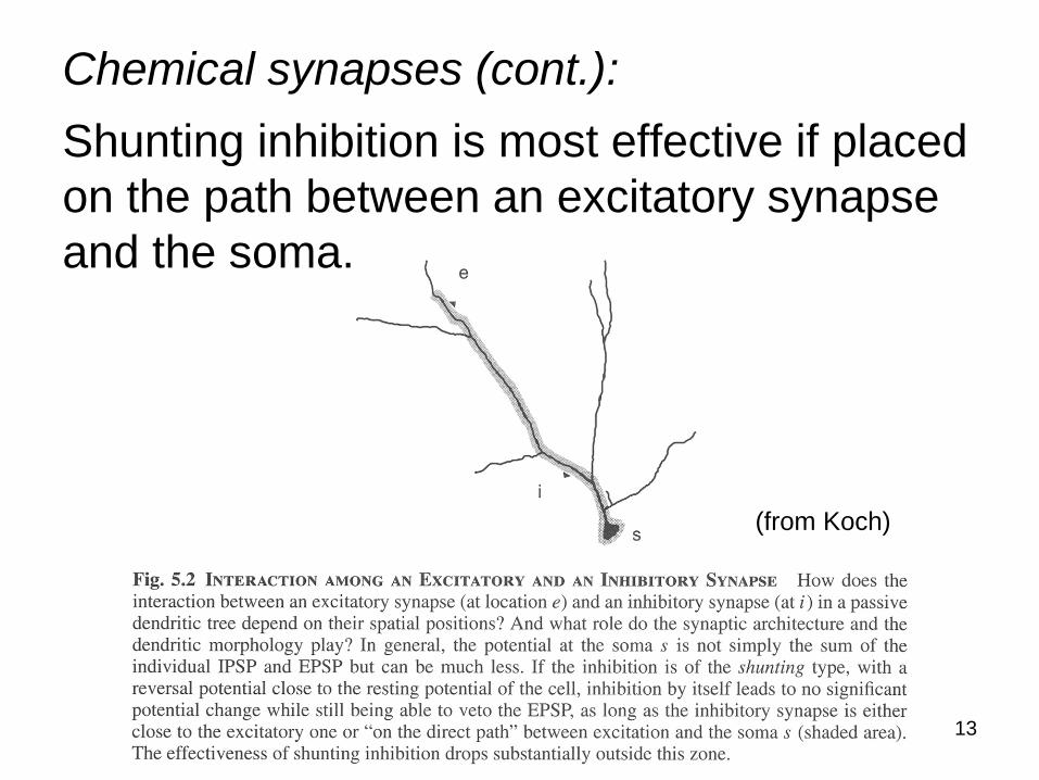
Chemical synapses (cont.): Shunting inhibition is most effective if placed on the path between an excitatory synapse and the soma.

(from Koch)

14

Chemical synapses (cont.):

(from Hille)

15

Chemical synapses (cont.): The maximum conductance gpeak is not fixed in many synapses. Rather, the efficiency of a synapse can be increased or decreased, depending on the pattern of synaptic input and/or whether an EPSP produced a spike in the post synaptic neuron. An increase in synaptic efficiency is referred to as long term potentiation (LTP), while a decrease is known as long term depression (LTD). These are forms of neural plasticity.

16

Receptor gating kinetics:

(from Hille)

17

Receptor gating kinetics (cont.): What causes the rate of exponential decay in the synaptic current of ligand-gated channels of fast chemical synapses?

A. The rate at which the neurotransmitter leaves the synaptic cleft?

B. The rate at which the channel naturally closes?

18

Receptor gating kinetics (cont.): A. The rate at which the neurotransmitter

leaves the synaptic cleft? Apparently not! 1. The rate of decay shown in Fig. 6.5 of

Hille is voltage dependent, which should not occur for a chemical diffusion process.

2. The rate of decay is temperature dependent, with a Q10 of 2.8, which is too high for a chemical diffusion process.

19

Receptor gating kinetics (cont.):

B. The rate at which the channel naturally closes?

If so, then the process might be modelled with the following kinetics:

(H6.1)

20

Receptor gating kinetics (cont.): From Eqn. (6.1) of Hille, it would be predicted that for a constant concentration of neurotransmitter in the synaptic cleft, such that the binding and unbinding of neurotransmitter is in equilibrium, then fluctuations should still be observed in the synaptic current with the same rate of decay. This is indeed the case, as illustrated in the next two slides.

21

Receptor gating kinetics (cont.):

(from Hille)

22

Receptor gating kinetics (cont.):

(from Hille)

23

Receptor gating kinetics (cont.): The power spectrum of an exponential decay has the form: where fc = 1/(2¼¿) corresponds to the −3dB cutoff frequency. The values of ¿ determined from this method match the values of ¿ obtained for synaptic input, supporting the proposed model.

24

Receptor gating kinetics (cont.): Further improvements on the model given by Eqn. (6.1) of Hille have consequently been developed. 1. The postsynaptic receptor may require

binding of more than one neurotransmitter molecular, e.g., two ACh molecules per ACh receptor.

2. The neurotransmitter unbinding process is slow, such that gaps can appear in the conductance of single ACh receptor currents.

25

Receptor gating kinetics (cont.): The refined kinetic model is:

(H6.3)

(from Hille)

26

Receptor gating kinetics (cont.): A structural model of gating of the ACh receptor has been proposed.

(from Gay and Yakel, J. Physiol. 2007)

27

Receptor gating kinetics (cont.): Possible gating movements of the ACh receptor protein upon agonist binding:

(from Gay and Yakel, J. Physiol. 2007)

28

Gap junctions in cardiac cells:

29

Gap junctions in cardiac cells (cont.):

30

Gap junctions in cardiac cells (cont.): Cable analysis of Purkinje fibers gives λ ¼ 1 mm and τ = 18 ms.

31

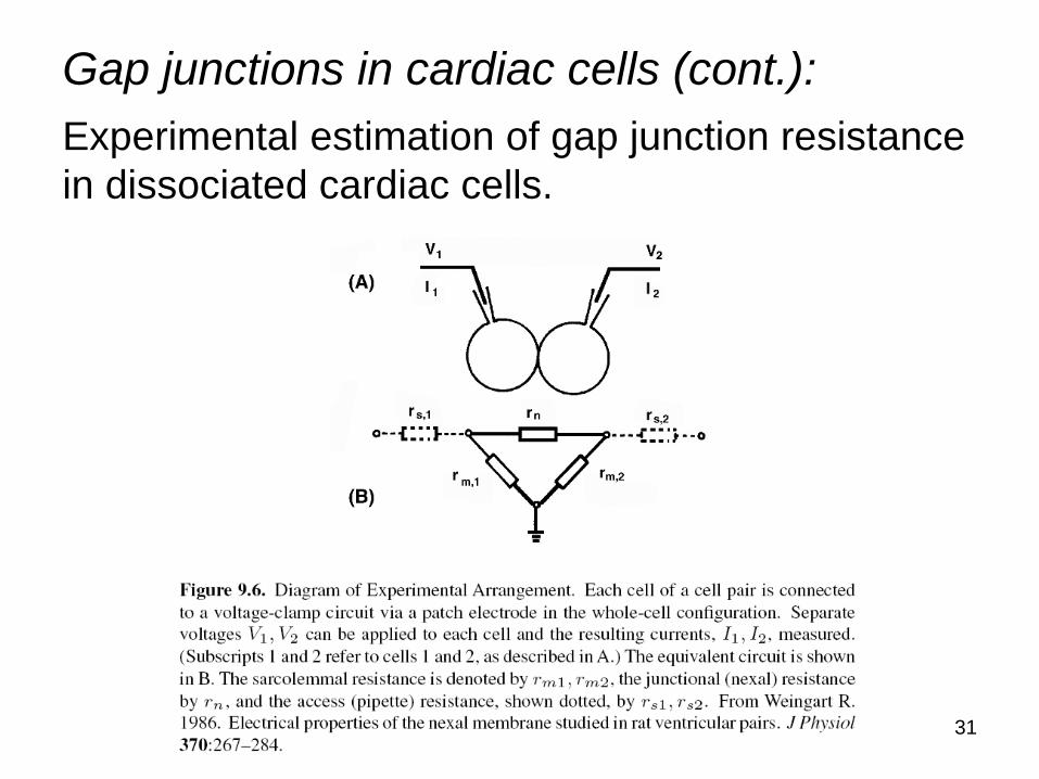
Gap junctions in cardiac cells (cont.): Experimental estimation of gap junction resistance in dissociated cardiac cells.

32

Gap junctions in cardiac cells (cont.):

33

Gap junctions in cardiac cells (cont.): Estimation of gap junction resistance in chick embryo cell pairs.

34

Gap junctions in nervous tissue: Gap junctions are found between :- – some neurons, mainly during

development, – glial cells, and – glial cells & neurons.

For more details, see: Brain Research Reviews 32(1), 2000.

35

8. DENDRITIC TREES

We will look at:

Properties of infinite, semi-infinite & finite cables

Branching in passive dendritic trees

Equivalent cylinder of a dendritic tree

Compartmental modeling

36

(from Koch)

Dendritic tree morphology:

37

Steady-state response of a finite cable: The steady-state response of a cable of finite length l in absolute units (or L = l/λ in electrotonic units) can be described by one of the equivalent forms: where:

38

Input impedance of a semi-infinite cable: Consider a current that is injected into the intracellular space at the origin of a semi-infinite cable (i.e., starts at x = 0 and heads off only in one direction to x = +1), with the return electrode in the extracellular space at the origin. The input impedance for the semi-infinite cable is:

39

Input impedance of a semi-infinite cable (cont.): For a semi-infinite cable the relative membrane potential is:

Assuming re ¼ 0, the intracellular axial current is:

40

Input impedance of a semi-infinite cable (cont.): Since λ ¼ (rm/ri)

1/2 when re ¼ 0: and the input impedance is:

41

Input impedance of a finite cable: The input impedance Zin for a finite cable will depend on the cable’s: length (l in absolute units, or L = l/λ in

electrotonic units), and termination impedance (ZL).

42

Input impedance of a finite cable: The termination impedance is determined by the physical configuration of the end of the fiber. Some common boundary conditions include: semi-infinite cable, sealed-end, killed-end, and arbitrary-impedance.

43

Input impedance of a finite cable (cont.): A semi-infinite cable termination of a

finite cable corresponds to ZL = Z0. In this case, the finite cable is simply considered to be the proximal section of a semi-infinite cable.

44

Input impedance of a finite cable (cont.): A sealed-end termination corresponds to

having a patch of membrane covering the end of the fiber, such that ZL ¼ 1. In this case, the internal axial current must be zero at the end of the fiber, i.e., Ii(X=L) = 0.

Using this boundary condition:

45

Input impedance of a finite cable (cont.): In the case of a sealed-end termination, the shorter the finite cable, the greater the effect of the infinite termination impedance on the input impedance.

46

Input impedance of a finite cable (cont.): A killed-end termination corresponds to

having a direct opening to the extracellular fluid at the end of the fiber, such that ZL ¼ 0. In this case, the transmembrane potential must be zero at the end of the fiber, i.e., Vm(X=L) = 0.

Using this boundary condition:

47

(from Koch)

Input impedance of a finite cable (cont.):

48

Input impedance of a finite cable (cont.): An arbitrary-impedance termination is

often used to describe the boundary between parent and daughter branches in dendritic trees.

Using this boundary condition:

49

Steady-state response of a finite cable:

(from Koch)

50

(from Koch)

Time-dependent response of a finite cable:

51

(from Koch)

Branching in passive dendritic trees:

52

Branching in passive dendritic trees (cont.): Assuming sealed ends on the daughter branches 1 and 2, their input impedances are: respectively. Thus, the parallel daughter branches are equivalent to a termination impedance given by:

53

Branching in passive dendritic trees (cont.): Consequently, the input impedances of the parent branch is: Multiple branches can be solved recursively in this manner.

54

Branching in passive dendritic trees (cont.): Once the input impedance at the site of current inject is calculated, the voltage at this site can be determined via: and given V0, we can compute the voltage at any point in the tree. This is achieved by calculating how much current flows into each of the daughter branches.

55

Branching in passive dendritic trees (cont.): In daughter branch 1: Thus:

) the current divides between the daughter

branches according to the input conductances

56

(from Koch)

Equivalent cylinder of a dendritic tree: Assume L1 = L2 and d1 = d2

57

Equivalent cylinder of a dendritic tree (cont.): In the case of d0

3/2 = 2d13/2, all derivatives of

the voltage profile are continuous ) the voltage decay can be described by a single expression. Why?

58

Equivalent cylinder of a dendritic tree (cont.): For a semi-infinite cable: If d0

3/2 = 2d13/2:

) Input impedances are matched

59

Equivalent cylinder of a dendritic tree (cont.): Consequently: and: ) A parent branch of length L0 with two identical

impedance-matched daughter branches of length L1 is equivalent to a single cylinder of length L0 + L1.

60

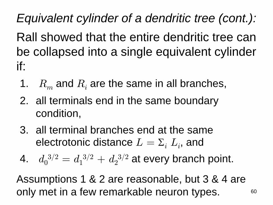
Equivalent cylinder of a dendritic tree (cont.): Rall showed that the entire dendritic tree can be collapsed into a single equivalent cylinder if: 1. Rm and Ri are the same in all branches, 2. all terminals end in the same boundary

condition, 3. all terminal branches end at the same

electrotonic distance L = Σi Li, and 4. d0

3/2 = d13/2 + d2

3/2 at every branch point.

Assumptions 1 & 2 are reasonable, but 3 & 4 are only met in a few remarkable neuron types.

61

(from Koch)

Compartmental modeling: