EE402 - Discrete Time Systems Spring 2018

Lecture 11Lecturer: Asst. Prof. M. Mert Ankarali

..

Frequency Response in Discrete Time Control Systems

Let’s assume u[k], y[k], and G(z) represents the input, output, and transfer function representation of aninput-output discrete time system.

In order to characterize frequency response of a discret system, the test signal is

u[k] = ejωk

which is an artificial complex periodic signal with a DT domain frequency of ω. The z-transform of u[k]takes the form

U(z) = Z{ejωk} =z

z − ejω

Response of the system in z-domain is given by

Y (z) = G(z)U(z) = G(z)z

z − ejω

Assuming that G(z) is a rational transfer function we can perform a partial fraction expansion

Y (z) =az

z − ejω + [terms due to the poles of G(z)]

a = limz→ejω

[(z − ejω)

Y (z)

z

]= G(ejω)

Y (z) =G(ejω)z

z − ejω + [terms due to the poles of G(z)]

Taking the inverse z-transform yields

y(t) = G(ejω)ejωk + Z−1 [terms due to the poles of G(z)]

If we assume that the system is “stable” or system is a part of closed loop system and closed loop behavioris stable then at steady state we have

yss[k] = G(ejω)ejωk

= |G(ejω)|eiωk+∠G(ejω)

= Meiωk+θ

In other words complex periodic signal is scaled and phase shifted based on the following operators

M = |G(ejω)|θ = ∠G(ejω

11-1

11-2 Lecture 11

It is very easy to show that for a general real time domain signal u[k] = sin(ωk + φ), the output y[k] atsteady state is computed via

yss[k] = M sin(ωk + φ+ θ)

If there is sampling involved in the system the following relation between DT frequency and CT frequencyexists ωd = ωcT

Similar to CT systems we utilize bode polts (or FRF function polts) to analyze DT systems and designfilter/controllers. Main difference between CT and DT bode polt is that while the frequency goes to infinityfor CT bode polts, for DT systems the frequency goes up-to π rad or ωs/2 (i.e. Nyquist frequency). Giventhe bode polt one can extract the magnitude scale and phase difference with respect to any input frequency.

Example: Let’s assume that we have the following CT plant transfer function

G(s) =1

s+ 1

The pulse transfer function of the following discretized system can be computed as

G(z) = Z[

1− e−Tss

1

s+ 1

]

x(t)

T ZOHy[k]

G(s) Tx[k]

We can also transform this DT transfer function to an artificial CT form using Bilinear-Tustin transformation.

G(s̄) = G(z)|z=

1+(T/2)s̄1−(T/2)s̄

Now let’s draw the bode plots of G(s), G(z), and G(s̄) for both T = 0.01s and T = 0.001s.

Lecture 11 11-3

Mag

nitu

de (d

B)

-60

-50

-40

-30

-20

-10

0

10-2 10-1 100 101 102 103 104

Phas

e (d

eg)

-180

-135

-90

-45

0

Mag

nitu

de (d

B)

-60

-50

-40

-30

-20

-10

0

10-2 10-1 100 101 102 103 104

Phas

e (d

eg)

-180

-135

-90

-45

0

T = 0.001 s ( ωs = 1 kHz )

Frequency (rad/s)

T = 0.01 s ( ωs = 100 Hz )

11-4 Lecture 11

Phase and Gain Margins

We already know that a binary stability metric is not enough the characterize the system performanceand that we need metrics to evaluate how stable the system is and its robustness to perturbations. Usingroot-locus techniques we talked about some “good” pole regions which provides some specifications aboutstability and closed-loop performance.

Another common and powerful method is the use gain and phase margins based on the Frequency ResponseFunctions of a closed-loop topology. Phase and gain margins are derived from the Nyquists stability criterionand it is relatively easy compute them from the Bode diagrams.

Gain Margin

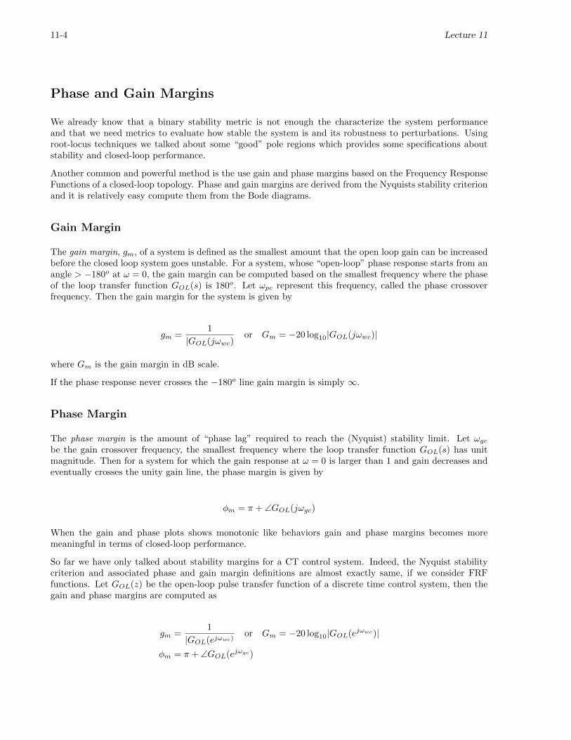
The gain margin, gm, of a system is defined as the smallest amount that the open loop gain can be increasedbefore the closed loop system goes unstable. For a system, whose “open-loop” phase response starts from anangle > −180o at ω = 0, the gain margin can be computed based on the smallest frequency where the phaseof the loop transfer function GOL(s) is 180o. Let ωpc represent this frequency, called the phase crossoverfrequency. Then the gain margin for the system is given by

gm =1

|GOL(jωwc)or Gm = −20 log10|GOL(jωwc)|

where Gm is the gain margin in dB scale.

If the phase response never crosses the −180o line gain margin is simply ∞.

Phase Margin

The phase margin is the amount of “phase lag” required to reach the (Nyquist) stability limit. Let ωgcbe the gain crossover frequency, the smallest frequency where the loop transfer function GOL(s) has unitmagnitude. Then for a system for which the gain response at ω = 0 is larger than 1 and gain decreases andeventually crosses the unity gain line, the phase margin is given by

φm = π + ∠GOL(jωgc)

When the gain and phase plots shows monotonic like behaviors gain and phase margins becomes moremeaningful in terms of closed-loop performance.

So far we have only talked about stability margins for a CT control system. Indeed, the Nyquist stabilitycriterion and associated phase and gain margin definitions are almost exactly same, if we consider FRFfunctions. Let GOL(z) be the open-loop pulse transfer function of a discrete time control system, then thegain and phase margins are computed as

gm =1

|GOL(ejωwc)or Gm = −20 log10|GOL(ejωwc)|

φm = π + ∠GOL(ejωgc)

Lecture 11 11-5

where as definitions of gain and phase crossover frequencies are exactly same.

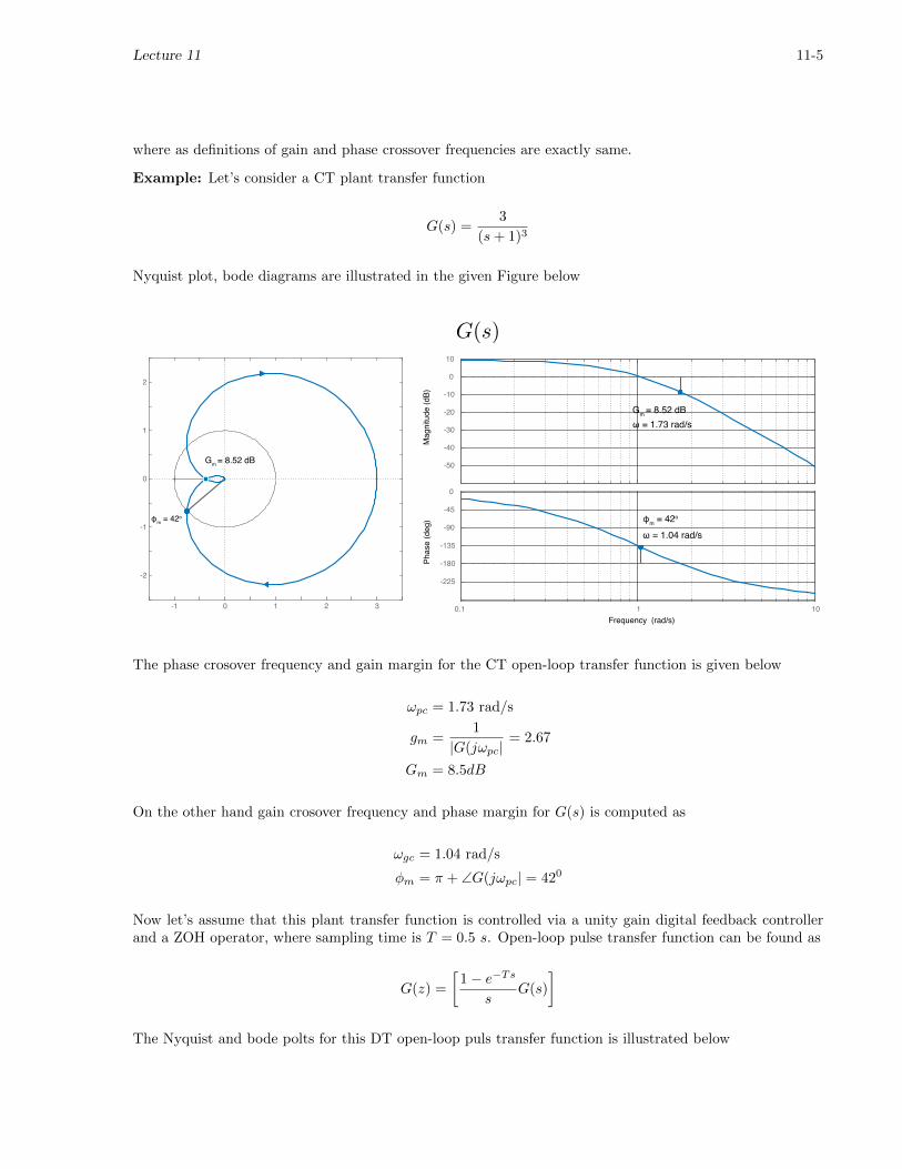
Example: Let’s consider a CT plant transfer function

G(s) =3

(s+ 1)3

Nyquist plot, bode diagrams are illustrated in the given Figure below

-1 0 1 2 3

-2

-1

0

1

2

Gm = 8.52 dB

φm = 42o

-50

-40

-30

-20

-10

0

10

Mag

nitu

de (d

B)

0.1 1 10

-225

-180

-135

-90

-45

0

Phas

e (d

eg)

Frequency (rad/s)

Gm = 8.52 dBω = 1.73 rad/s

ω = 1.04 rad/sφm = 42o

The phase crosover frequency and gain margin for the CT open-loop transfer function is given below

ωpc = 1.73 rad/s

gm =1

|G(jωpc|= 2.67

Gm = 8.5dB

On the other hand gain crosover frequency and phase margin for G(s) is computed as

ωgc = 1.04 rad/s

φm = π + ∠G(jωpc| = 420

Now let’s assume that this plant transfer function is controlled via a unity gain digital feedback controllerand a ZOH operator, where sampling time is T = 0.5 s. Open-loop pulse transfer function can be found as

G(z) =

[1− e−Ts

sG(s)

]

The Nyquist and bode polts for this DT open-loop puls transfer function is illustrated below

11-6 Lecture 11

-1 0 1 2 3

-2

-1

0

1

2

Gm = 4.18 dB

φm = 28o

-40

-30

-20

-10

0

10

Mag

nitu

de (d

B)

0.1 1 10

-270

-180

-90

0

Phas

e (d

eg)

Frequency (rad/s)

Gm = 4.18 dBω = 1.35 rad/s

ω = 1.03 rad/sφm = 28o

Note that instead of DT frequency ωd ∈ [0, pi), the x-axis illustrates the actual frequency ω = ωd/T . Isvery easy to associate DT and CT frequencies, and main advantage of actual frequency is that CT and DTversions of bode plots becomes directly comparable.

The phase crosover frequency and gain margin for the DT open-loop transfer function is given below

ωpc = 1.35 rad/s

gm =1

|G(ejωpcT |= 1.62

Gm = 4.18dB

On the other hand gain crosover frequency and phase margin for G(s) is computed as

ωgc = 1.03 rad/s

φm = π + ∠G(jωpc| = 280

If we compare the CT and DT versions of the same system, we can see that both gain margin and phasemargin of the original CT system is better, and we can conclude that discretization reduces the “stability”.Another interesting result is that while there is a significant change in phase-crossover frequency, the changein gain crosover frequency is minimal.

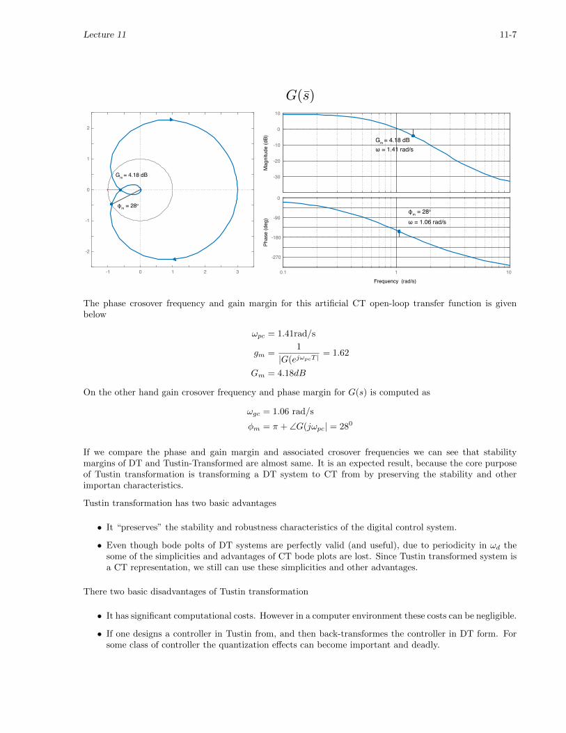
Now let’s transfrom the G(z) to a artificial CT system using Bilinear-Tustin transformation:

G(s̄) = G(z)|z=

1+(T/2)s̄1−(T/2)s̄

We know that the relation between the frequency of this artificial system, ω̄, and frequencies of the actualsystem and discretized system are given by

ω̄ =2

Ttan(

ωd2

) =2

Ttan(

ωT

2)

Lecture 11 11-7

-1 0 1 2 3

-2

-1

0

1

2

Gm = 4.18 dB

φm = 28o

Frequency (rad/s)

-30

-20

-10

0

10

Mag

nitu

de (d

B)0.1 1 10

-270

-180

-90

0

Phas

e (d

eg)

Gm = 4.18 dBω = 1.41 rad/s

ω = 1.06 rad/sφm = 28o

The phase crosover frequency and gain margin for this artificial CT open-loop transfer function is givenbelow

ωpc = 1.41rad/s

gm =1

|G(ejωpcT |= 1.62

Gm = 4.18dB

On the other hand gain crosover frequency and phase margin for G(s) is computed as

ωgc = 1.06 rad/s

φm = π + ∠G(jωpc| = 280

If we compare the phase and gain margin and associated crosover frequencies we can see that stabilitymargins of DT and Tustin-Transformed are almost same. It is an expected result, because the core purposeof Tustin transformation is transforming a DT system to CT from by preserving the stability and otherimportan characteristics.

Tustin transformation has two basic advantages

• It “preserves” the stability and robustness characteristics of the digital control system.

• Even though bode polts of DT systems are perfectly valid (and useful), due to periodicity in ωd thesome of the simplicities and advantages of CT bode plots are lost. Since Tustin transformed system isa CT representation, we still can use these simplicities and other advantages.

There two basic disadvantages of Tustin transformation

• It has significant computational costs. However in a computer environment these costs can be negligible.

• If one designs a controller in Tustin from, and then back-transformes the controller in DT form. Forsome class of controller the quantization effects can become important and deadly.

11-8 Lecture 11

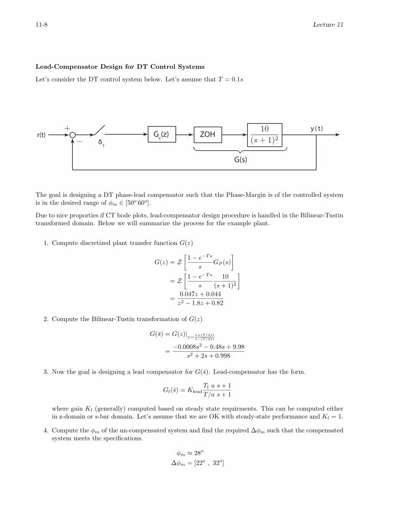
Lead-Compensator Design for DT Control Systems

Let’s consider the DT control system below. Let’s assume that T = 0.1s

+

−r(t) Gc(z)

y ( t)ZOH

δT

G(s)

The goal is designing a DT phase-lead compensator such that the Phase-Margin is of the controlled systemis in the desired range of φm ∈ [50o 60o].

Due to nice proporties if CT bode plots, lead-compensator design procedure is handled in the Bilinear-Tustintransformed domain. Below we will summarize the process for the example plant.

1. Compute discretized plant transfer function G(z)

G(z) = Z[

1− e−Tss

GP (s)

]= Z

[1− e−Ts

s

10

(s+ 1)2

]=

0.047z + 0.044

z2 − 1.8z + 0.82

2. Compute the Bilinear-Tustin transformation of G(z)

G(s̄) = G(z)|z=

1+(T/2)s̄1−(T/2)s̄

=−0.0008s2 − 0.48s+ 9.98

s2 + 2s+ 0.998

3. Now the goal is designing a lead compensator for G(s̄). Lead-compensator has the form.

Gl(s̄) = KleadTl a s+ 1

T/a s+ 1

where gain Kl (generally) computed based on steady state requirments. This can be computed eitherin z-domain or s-bar domain. Let’s assume that we are OK with steady-state performance and Kl = 1.

4. Compute the φm of the un-compensated system and find the required ∆φm such that the compensatedsystem meets the specifications.

φm ≈ 28o

∆φm = [22o , 32o]

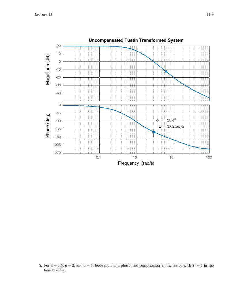
Lecture 11 11-9

-40

-30

-20

-10

0

10

20M

agni

tude

(dB)

0.1 10 10 100-270

-225

-180

-135

-90

-45

0

Phas

e (d

eg)

Uncompansated Tustin Transformed System

Frequency (rad/s)

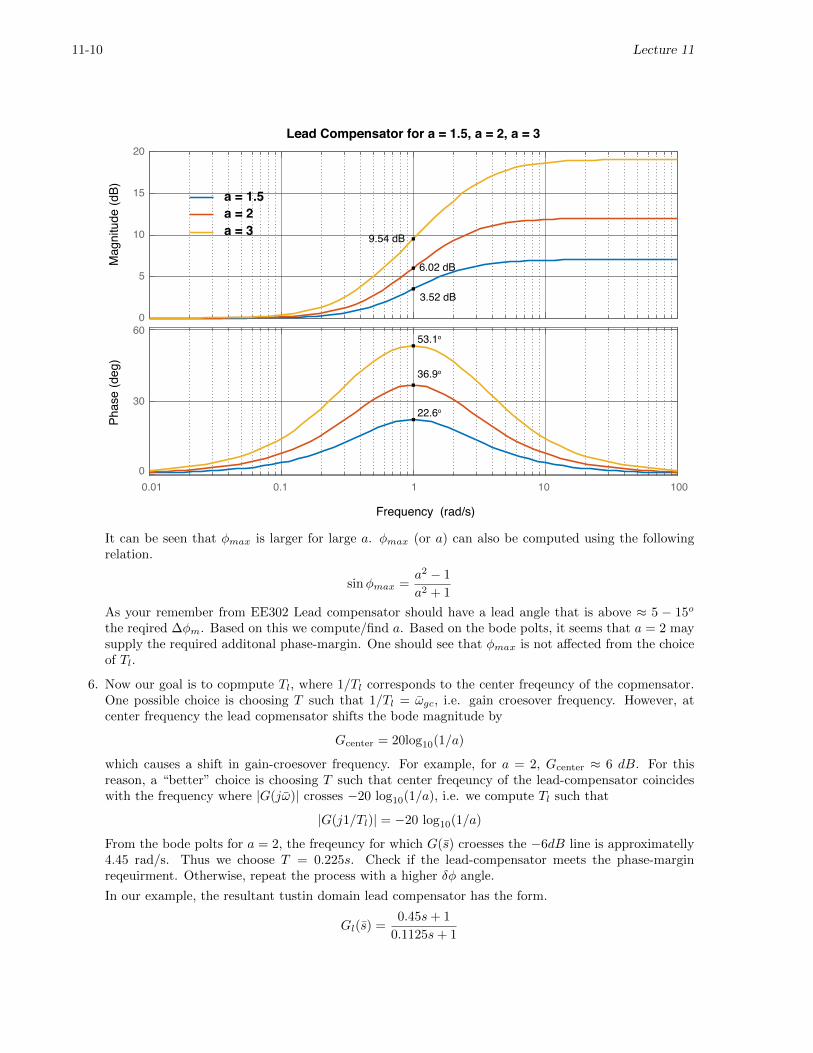
5. For a = 1.5, a = 2, and a = 3, bode plots of a phase-lead compensator is illustrated with Tl = 1 in thefigure below.

11-10 Lecture 11

0

5

10

15

20

Mag

nitu

de (d

B)

0.01 0.1 1 10 1000

30

60

Phas

e (d

eg)

Lead Compensator for a = 1.5, a = 2, a = 3

Frequency (rad/s)

22.6o

36.9o

53.1o

9.54 dB

6.02 dB

3.52 dB

a = 1.5

a = 3a = 2

It can be seen that φmax is larger for large a. φmax (or a) can also be computed using the followingrelation.

sinφmax =a2 − 1

a2 + 1

As your remember from EE302 Lead compensator should have a lead angle that is above ≈ 5 − 15o

the reqired ∆φm. Based on this we compute/find a. Based on the bode polts, it seems that a = 2 maysupply the required additonal phase-margin. One should see that φmax is not affected from the choiceof Tl.

6. Now our goal is to copmpute Tl, where 1/Tl corresponds to the center freqeuncy of the copmensator.One possible choice is choosing T such that 1/Tl = ω̄gc, i.e. gain croesover frequency. However, atcenter frequency the lead copmensator shifts the bode magnitude by

Gcenter = 20log10(1/a)

which causes a shift in gain-croesover frequency. For example, for a = 2, Gcenter ≈ 6 dB. For thisreason, a “better” choice is choosing T such that center freqeuncy of the lead-compensator coincideswith the frequency where |G(jω̄)| crosses −20 log10(1/a), i.e. we compute Tl such that

|G(j1/Tl)| = −20 log10(1/a)

From the bode polts for a = 2, the freqeuncy for which G(s̄) croesses the −6dB line is approximatelly4.45 rad/s. Thus we choose T = 0.225s. Check if the lead-compensator meets the phase-marginreqeuirment. Otherwise, repeat the process with a higher δφ angle.

In our example, the resultant tustin domain lead compensator has the form.

Gl(s̄) =0.45s+ 1

0.1125s+ 1

Lecture 11 11-11

The Figure below illiustrates the bode plots of both (tustin domain) compensated and uncompansatedsystems. Compensated systems has a phase margin of φm = 51o which meets the requirements.

-40

-30

-20

-10

0

10

20

Mag

nitu

de (d

B)

0.1 1 10 100

-225

-180

-135

-90

-45

0

Phas

e (d

eg)

Compansated Tustin Domain System

Frequency (rad/s)

7. Transform the s̄-domain lead-compensator to z-domain.

Gl(z) =Gl(s̄)|s̄= 2T

z−1z+1

Gl(z) =3.08z − 2.46

z − 0.385

8. Check if the discrete-time compensator meets the the phse-margin requirments.

11-12 Lecture 11

-50

-40

-30

-20

-10

0

10

20

Mag

nitu

de (d

B)

0.01 1 10 100

-225

-180

-135

-90

-45

0

Phas

e (d

eg)

Compansated and Uncompansated Open-Loop Pulse Transfer Functions

Frequency (rad/s)

It can be seen that the designed compensator in z-domain also meets the phase-margin specifications.

In Figure below, we compare the closed-loop step responses of both uncompensated and compensated pulsetransfer functions.

Lecture 11 11-13

0 1 2 3 4 5 6 7 80

0.2

0.4

0.6

0.8

1

1.2

1.4Step Resposes - Compensated (Red) and Uncompansated (Blue)

Time (seconds)

Ts = 5.1 s

OS = %48

Ts = 1.3 s

OS = %25