ES 442 Lecture 1 1

EE442 Introduction(A gentle and brief introduction)

EE442 Analog & Digital Communication Systems

Lecture 1

Assignment: Read Chapter 1 of Agbo & Sadiku

Principles of Modern Communication Systems

Textbook: Samuel O. Agbo and Matthew N. O. SadikuPrinciples of Modern Communication Systems

Cambridge University Press, 2017.

ES 442 Lecture 1 2

Definition of a Communication System (from Section 1.1)

A “communication system” is an apparatus that conveys information from a source (the transmitter) to a destination (the receiver) over a channel (the propagation medium carrying the signal).

Common sources of Information:

• Audio/voice – information in acoustic form• Text messages – written text sent in digital format• Data – computer generated information in digital format• Video -- electronic representation of images or pictures

Categories of information: Analog and Digital

Refer to Section 1.3, pages 3 to 6.

Signals Carry Content in Communication Systems

3EE 442 Lecture 1

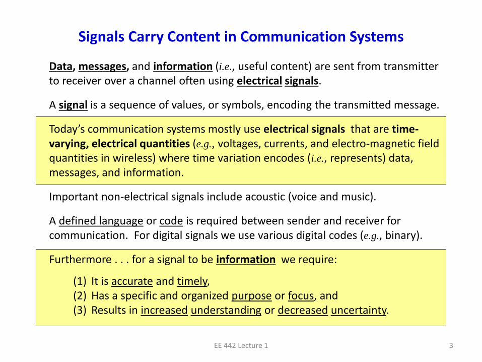
Data, messages, and information (i.e., useful content) are sent from transmitter to receiver over a channel often using electrical signals.

A signal is a sequence of values, or symbols, encoding the transmitted message.

Today’s communication systems mostly use electrical signals that are time-varying, electrical quantities (e.g., voltages, currents, and electro-magnetic field quantities in wireless) where time variation encodes (i.e., represents) data, messages, and information.

Important non-electrical signals include acoustic (voice and music).

A defined language or code is required between sender and receiver for communication. For digital signals we use various digital codes (e.g., binary).

Furthermore . . . for a signal to be information we require:

(1) It is accurate and timely,(2) Has a specific and organized purpose or focus, and(3) Results in increased understanding or decreased uncertainty.

EE 442 Lecture 1 4

The Four Great Enablers of the Communication Age(from ES 101A “Communications in the Information Age”)

Electric PowerGeneration (1880s)

Alessandra

Volta – Battery(1800)

1. Harnessing of Electricity

Guglielmo MarconiRadio Waves

( began in 1896 withwireless telegraphy )

2. Radio Waves

3. Digitization 4. Transistors& IntegratedCircuits

Telegraph & Telephone1844 1876

Started in 1940s(but accelerated

in the 1970s) Moore’s Law

Transistor 1948IC invented 1958

(Jack Kilby & Robert Noyce)

Source: D. B. Estreich from ES101

EE 442 Lecture 1 5

Selective History of Communication Technologies

1794 – Claude Chappe develops an armature signal telegraph1837 – Samuel Morse independently develops and patents an

electrical telegraph (leads to Morse Code)1876 – Alexander Graham Bell demonstrates voice-based telephone 1896 – Wireless telegraphy (radio telegraphy) by Guglielmo Marconi1901 – First transatlantic radio telegraph transmission (Marconi)1906 – First AM radio broadcast by Reginald Fessenden1920 – First commercial radio stations in US1921 – First mobile radio service (Detroit Police Department)1928 – First television station in United States (W3XK)1935 – Edwin Armstrong demonstrates FM radio 1947 – Bell Telephone Laboratories (BTL),proposed cellular concept1947 – BTL invents and demonstrates solid-state transistor1958 – Integrated circuit invented (Kilby at TI & Noyce at Fairchild)1980s – Fiber optic technology developed1984 – Analog AMPS cellular mobile service by Motorola1991 – GSM cellular service (digital) service begins1997 – IEEE 802.11(b) wireless LAN standard

Table 1.1 (pp. 4-5) lists other milestones in communication.

ES 442 Lecture 1 6

Claude Chappe (1793) Semaphore Telegraph System

http://thepublici.blogspot.com/2009/06/

parcel-post.html

Télégraphe means “far writer”

http://cabinet-of-

wonders.blogspot.com/2007/11/semaphore-as-

information-network.html

Next

Station

ES 442 Lecture 1 7

Communication Network of French Telegraph by 1820

And by 1852, the

network of optical

telegraphs in France

alone had grown to 556

telegraph stations,

covering 4,800 km

(3,000 miles). This

network connected 29

of France's largest

cities to Paris. With

two operators on duty

at each station and

employed over 1,000

people. 196 different

signals (arm

positions) were used

to send about two

words per minute.

http://www.royal-signals.org.uk/Datasheets/Telegraph%20.php

Paris

France

ES 442 Lecture 1 8

What Communication Technology does this describe?

1. It demonstrated the “power of communication”2. Its impact was Worldwide3. It made the world smaller by instantaneous communication 4. It revolutionized and created new industries5. Altered business: E-commerce became important 6. Security and privacy became very important issues 7. It gave new hope for peacemaking and diplomacy 8. Its technicians and operators became an elite group9. New forms and schemes of fraud emerged

One of the Great Communication Milestones

ES 442 Lecture 1 9

What Communication Technology does this describe?

ANSWER: The Electric Telegraph (aka Victorian Internet)

Reference: Tom Sandage, The Victorian Internet, Walker & Company, 1998.

One of the Greatest Communication Milestones

http://public.beuth-hochschule.de/hamann/telegraf/index.html

ES 442 Lecture 1 10

Charles Wheatstone & William Cooke developedthe first demonstrated electrical telegraph.

It was a “Five-needle telegraph” (1837) as shown

below. There were two disadvantages: (1) it usedand 20-character alphabet, and (2) it needed six parallel wires for operation. First commercial use in1838 between railroad stations.

Supported20 lettersalphabet

Wheatstone-CookeTelegraph

A

B D

E F G

H KI L

M N

R

O P

S T

U

Y

W

http://www.sciencemuseum.org.uk/images/I039/10307306.aspx

6 wires

Wheatstone & Cook Telegraph Preceded Morse Telegraph

EE 442 Lecture 1 11

The Telegraph Revolution

➢ Near instantaneous communication➢ Adopted worldwide➢ Became the Victorian Internet➢ Used by railroads, newspapers,

financial organizations, businesses of all kinds,

➢ Used in the Civil War by both Northand South

Samuel Morse 1844

ES 442 Lecture 1 12

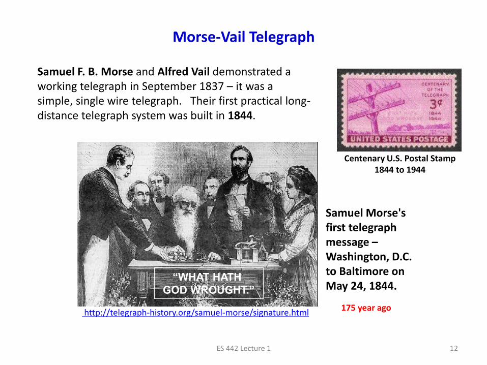
Samuel F. B. Morse and Alfred Vail demonstrated a working telegraph in September 1837 – it was a simple, single wire telegraph. Their first practical long-distance telegraph system was built in 1844.

Centenary U.S. Postal Stamp1844 to 1944

http://telegraph-history.org/samuel-morse/signature.html

Samuel Morse's first telegraph message –Washington, D.C. to Baltimore on May 24, 1844.

“WHAT HATH

GOD WROUGHT.”

175 year ago

Morse-Vail Telegraph

ES 442 Lecture 1 13

http://www.sonofthesouth.net/leefoundation/civil-war/1863/january/telegraph.htm

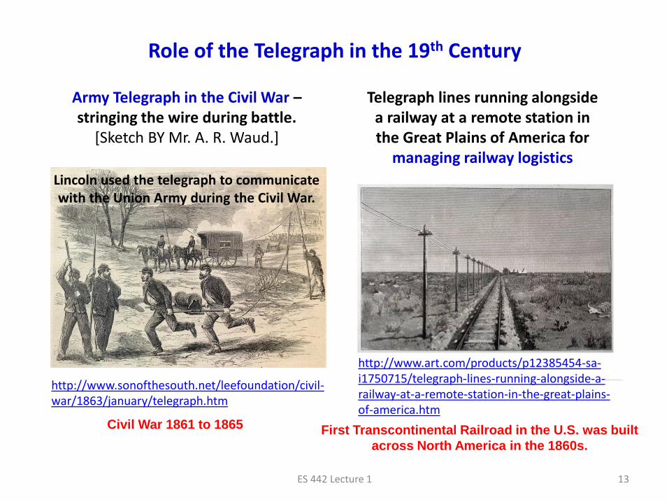
Telegraph lines running alongside a railway at a remote station in the Great Plains of America for

managing railway logistics

http://www.art.com/products/p12385454-sa-i1750715/telegraph-lines-running-alongside-a-railway-at-a-remote-station-in-the-great-plains-of-america.htm

Army Telegraph in the Civil War –stringing the wire during battle.

[Sketch BY Mr. A. R. Waud.]

Lincoln used the telegraph to communicatewith the Union Army during the Civil War.

Civil War 1861 to 1865 First Transcontinental Railroad in the U.S. was built

across North America in the 1860s.

Role of the Telegraph in the 19th Century

ES 442 Lecture 1 14

http://www.artvalue.com/auctionresult--hogarth-

william-1697-1764-unit-the-electioneering-series-4-

1899983.htm

Heliograph – a “wireless solar telegraph” that signals with flashes of sunlight

reflected by a mirror. The flashes are produced by momentarily pivoting the

mirror or interrupting the beam with a shutter and often use codes such as

Morse code.

Sir Henry Mance (British Army Signal Corps) developed first apparatus in 1869 in

India. The heliograph remained standard equipment in the Australian and British

armies until the 1960s. Also used by the U.S. Forrest Service. Longest heliograph

communication distance slightly greater than 200 miles.

http://en.wikipedia.org/wiki/Heliograph

Long Range Optical Communication

EE 442 Lecture 1 15

❑ Public Switched Telephone Network (PSTN) – voice, fax, modem

❑ Radio broadcasting (AM and FM)

❑ Citizens’ band radio; ham short-wave radio; radio control; etc.

❑ Computer networks (LANs, MANs, WANs, and Internet)

❑ Aviation communication bands; Emergency bands; etc.

❑ Satellite systems (Commercial and Military communications)

❑ Cable television (originally CATV) for video and data

❑ Cellular networks (4 generations – Now LTE or 4G → 5G)

❑ Wi-Fi LANs

❑ Bluetooth

❑ GPS

But Communication Systems Have Come A Long Ways

And of course many, many more . . . .

Transmitter will . . . Encode message data Add a carrier signal

(modulation) Set signal parameters for

channel transmissionand transmit

Receiver will . . . Receive signal Remove the carrier signal

(demodulation) Decode the data to put it

into format for destination

Information Source

Transmitter Information Destination

Receiver

Messagebeing sent

Messagereceived

SignalTransmitted

SignalReceived

NoiseMessage putinto a format

appropriate fortransmitting over channel

Signal retrievedfrom channel

and converted into a format

appropriate forthe destination

Wireline, EM waves

or Fiber

Noise distorts

signal withrandom

additions

Channel

Shannon-Weaver Model for Communication

16EE 442 Lecture 1

Refer toSection 1.3,particularly

page 5.

ES 442 Lecture 1 17

https://slideplayer.com/slide/7873541/

Sklar’s Model for Digital Communication

Bernard Sklar, Digital Communications: Fundamentals and Applications, 2nd ed., Prentice-Hall, New York, 2001.

EE 442 Lecture 1 18

Electrical/OpticalSignals

as used inCommunication

Systems

Electrical & Optical Signals Dominate Communication

ES 442 Lecture 1 19http://en.wikipedia.org/wiki/Carbon_microphone

Example: Human Speech is an Analog SignalV

olt

age

(V)

Front contact

Button

Back contact

Diaphragm

V

Sound

waves

Resistive carbon layer

+

─Bat

tery

Word: “erase”

Expanded view of voltage waveform

A microphone is a “transducer”

Carbon-Granular MicrophoneInventor: Thomas Edison 1877

voltage waveform

ES 442 Lecture 1 20

http://www.cisco.com/en/US/prod/collateral/voicesw/ps6788/phones/ps379/ps8537/prod_white_paper0900aecd806fa57a.html

0 Hz 300 Hz 3,400 Hz 4,000 Hz 7,000 Hz

Voice energy

Telephone BandFilter Shape

Voice Bandwidth300 Hz to 3,400 Hz

Voice Channel0 Hz to 4,000 Hz

Frequency f (Hz)

Ene

rgy

Voice Bandwidth (Bell Determined 3400 Hz Was Adequate)

ES 442 Lecture 1 21

FREQUENCY in Hertz (Hz)

20 50 100 200 500 1K 2K 5K 10K 20K

120

100

80

60

40

20

0SOU

ND

INTE

NSI

TY L

EVEL

ind

eci

be

ls (

dB

)

Human Hearing Chart

Discomfort Threshold

Speech

HearingThreshold

Music

aging

Presbycusis is loss of hearing with age.

Acoustic signals

Human Speech Intensity and Frequency Boundaries

Sound velocity 1100 ft/sec

ES 442 Lecture 1 22

Modern Communication Systems are Dominated by Wireless

cellularhttps://www.researchgate.net/figure/A-proposed-5G-heterogeneous-wireless-cellular-architecture_fig1_260523836

VLC is visible light communication

Cognitive Radio (CR)

EE 442 Lecture 1 23

Electromagnetic Spectrum (There is only one in the universe)

http://www.mondialbioregulator.co.uk/electromagnetic-spectrum-mondial-bioregulator.asp

The gateway to wireless

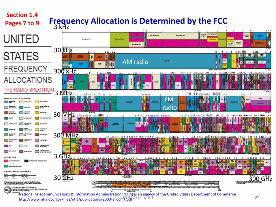
ES 442 Lecture 1 24National Telecommunications & Information Administration (NTIA) is an agency of the United States Department of Commercehttp://www.ntia.doc.gov/files/ntia/publications/2003-allochrt.pdf

AM radio

FMradio

3 kHz

300 GHz30 GHz

3 GHz

300 MHz

30 MHz

3 MHz

300 kHz

30 kHz

Frequency Allocation is Determined by the FCCSection 1.4Pages 7 to 9

ES 442 Lecture 1 25

Some Frequency Allocations of Interest in EE442

http://www.informit.com/articles/article.aspx?p=2249780

540 to 1720 kHz

88 to 108 MHz

2.402 to 2.484 GHz

174 to 216; 470 to 806 MHz

27.5 to 28.35 GHz

See next slide

ES 442 Lecture 1 26

http://unitedunlock.blogspot.com/2016/02/what-networks-are-compatible-with-my.html

Selected Frequency Allocations in Cellular TelephonyAll frequencies in megahertz (MHz)

EE 442 Lecture 1 27

Radio and Optical Windows in the Atmosphere

http://www.spaceacademy.net.au/spacelink/radiospace.htm

Just as sight depends upon the “Visible Window,” wireless communicationdepends upon the existence of the “Radio Window” in the EM spectrum.

Ozone &Molecular

Oxygen

Water &CarbonDioxide

ChargedParticles

Radio

Window

Frequency

Op

acit

y

Partial IR Windows

Visible Window

Microwave Windows

Increasing frequency

0 %

MHz PHzGHz THz

100 %

30 3003 30 3003 30 3003 303

EE 442 Lecture 1 28

Total, Dry Air and Water-vapor Zenith Attenuation at Sea Level

V-band is 50 to 75 GHzW-band is 75 to 100 GHz

W-band & V-band used in satellite communications

Why W/V band for satellite communications?

W & V bands have no crowding in frequency, hence, this provides reduced interference, large bandwidth availability, reduced antenna and electronic components size, and more security in point-to-point links due to smaller beamwidths.

Dry air

Water vapor

Total

Frequency (Hz)

1

0.1

0.01

10

100

1 10 100 3500.001

Zen

ith

Att

en

uat

ion

(d

B)

1000

Radio Window

V & W bands

EE 442 Lecture 1 29

Example: Unlicensed Spectrum – ISM and & UHII RF Bands

Band

ISM I

ISM II

ISM III

Frequency Range

902 – 928 MHz

2.4 – 2.4835 GHz

5.725 – 5.85 GHz

UNII I

UNII II

UNII III

5.15 – 5.25 GHz

5.25 – 5.35 GHz

5.725 – 5.875 GHz

Applications

Cordless phones; 1G Wireless Cellular

Wi-Fi; Bluetooth; ZigBee; Microwave ovens

Cordless phones; Wireless PBX

Wi-Fi 802.11a/n

Short-range indoor; Campus applications

Long-range outdoor; Point-to-Point links

ISM: Industrial, Scientific & Medical & UNII: Unlicensed National Information Infrastructure

Frequency (GHz)1

UNI IISM II

2 43 65

ISM I UNI IIISM IIIUNI III

ES 442 Lecture 1 30

Antennas are Crucial to Wireless Communication

Cellular base stationantennas

Yagi antenna

Parabolicantenna

Dipole antenna

Cell phone antenna

Mast antenna

EE 442 Lecture 1 31

Wireless Communication: Radiation from Dipole Antenna

Single Direction Shown Here

http://askthephysicist.com/ask_phys_q&a_old5.html

Dipoleantenna

dipole

Electric & Magnetic Fields

Far Field

Propagation

ES 442 Lecture 1 32

Fundamental Limitations in Electrical Communications

There are (1) Technological Constraints, and (2) Fundamental PhysicalConstraints.

There are two fundamental physical constraints:

(A) Bandwidth limitationRelated to how rapidly we can change signals (a change instored energy requires a non-zero amount of time). A goodmeasure of signal change speed is bandwidth.Also there are regulatory limits set by the FCC in the US.

(B) Noise limitationNoise is always present and it sets a lower signal level wherethe signal can be reliably detected. Sources of noise includeatmospheric noise, electromagnetic interference (RFI), galactic noise, thermal and shot noise in circuits and devices,and many others.

EE 442 Lecture 1 33

Channel Limitations and Challenges

❑ Propagation loss – The greater the distance, the greater the loss (All channels are lossy unless they have gain built into them)❑ Frequency selectivity – Most media are transmitted over selective frequency bands (FCC assigns these bands)❑ Time variation – Many channels have natural varying conditions which change transmission properties (e.g., temperature and moisture content changes; motion in objects)❑ Nonlinearity – Ideally a channel is linear; however, exceptions exist such as satellite communication through the ionosphere ❑ Shared usage – Most channels are not dedicated to a single user so they must contend with multiple users ❑ Noise – All channels contribute noise to the signal as it travels through the medium❑ Interference – Channels can pick up adjacent communication signals and noise which interfere with the intended signals

All of these influence and/or limit the choice of modulation schemes & transmitter/receiver (transceiver) design.

EE 442 Lecture 1 34

Radio Waves

Mobile Station: MS or UE

Also, Moisture in atmospherecauses attenuation in radio signal strength.

MultipathReception

BaseTransceiver

Station

Challenges in Wireless: Fading in Cellular Telephony

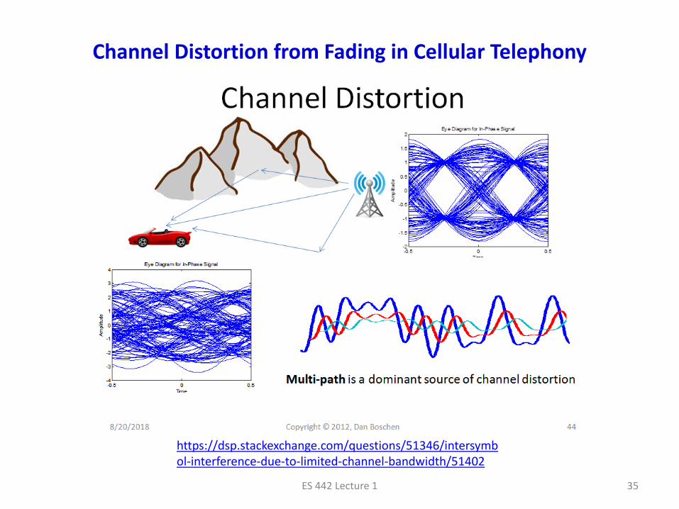
ES 442 Lecture 1 35

https://dsp.stackexchange.com/questions/51346/intersymbol-interference-due-to-limited-channel-bandwidth/51402

Channel Distortion from Fading in Cellular Telephony

EE 442 Lecture 1 36

Why do we cover Analog if Digital is so dominant today?

1. The world is fundamentally an analog world (People respond

primarily to analog symbols, images & sounds)

2. Digital signals are actually “analog signals” encoded as “digital data”

(e.g., bits still must be converted to physical waveforms)

3. Digital communication systems make use of components leveraged

from analog communication systems (e.g., ADC & DAC converters,

mixers, amplifiers, combiners, antennas, etc.)

4. Analog communication systems illustrate high-level issues and principles

(this is especially true as we push data rate limits higher)

5. Analog communication systems are still in use (e.g., AM and FM radio)

IMPACT: We must be able to convert analog to digital & vice versa.

ES 442 Lecture 1 37

time time

amp

litu

de

amp

litu

de

0 1 0 1 . . . 1 1 0 1

All signal waveforms are analog – the difference is what they represent!

Analog Signals versus Digital Signals

• Analog Signals represent the values of physical parameters which are time varying.

Amplitude can be any value within a range of values

Amplitude is time-varying

• Digital Signals represent a sequence of numbers.

The values restricted to a set of discrete values

Example: Binary signal with only two

values (1 and 0).

Amplitude is time-varying, but

absolute magnitude less important

EE 442 Lecture 1 38

Advantages of Digital Over Analog

1. Digital is more robust than analog to noise and interference†

2. Digital is more viable when using regenerative repeaters

3. Digital hardware is more flexible by using microprocessors and VLSI

4. Can be coded to yield extremely low error rates with error correction

5. Easier to multiplex several digital signals than analog signals

6. Digital is more efficient in trading off SNR for bandwidth

7. Digital signals are easily encrypted for security purposes

8. Digital signal storage is easier, cheaper and more efficient

9. Reproduction of digital data is more reliable without deterioration

10. Cost is coming down in digital systems faster than in analog systems and DSP algorithms are growing in power and flexibility

† Analog signals vary continuously and their value is affected by all levels of noise.

SNR = signal-to-noise ratio

DSP = digital signal processing

VLSI = very large-scale integration

EE 442 Lecture 1 39

Information Capacity (Shannon Capacity) – Noise Dependent❑ Data rate R is limited by channel bandwidth, signal power, noise

power and distortion in general

❑ Without distortion or noise, we could transmit without limit to the

data rate. However, this is never reality.

❑ The Shannon capacity C is the maximum possible data rate for a

system with noise and distortion

❑ Maximum rate approached with bit error probability close to 0. For

additive white Gaussian noise (AWGN) channels,

❑ Shannon obtained C = 32 kbps for telephone channels

❑ In practice we are nowhere near capacity limit in wireless systems

2C log 1 in bits per secondsignal power

Bnoise power

= +

Refer to Section 1.5 of Agbo & Sadiku; pages 10 to 12.

SNR

ES 442 Lecture 1 40

Nyquist Channel Capacity

https://www.slideshare.net/AvijeetNegel/data-communication-and-networking-data-rate-limits

2channel capacity (bits/sec) 2 ( )

where bandwidth (Hz)

and Number of bits/symbol

C B log M

B

M

= =

=

=

Known as the Nyquist Theorem

EE 442 Lecture 1 41

Additive White Gaussian Noise Corrupts Signals

“White” means noise power isuniform over all frequencies

Digital signal corrupted bywhite Gaussian noise

Hidden Signal

AWGN = Additive White Gaussian Noise

EE 442 Lecture 1 42

Digital Signal Errors From Noise and Interference

https://slideplayer.com/slide/13937000/

2 errors out of 15 bits

EE 442 Lecture 1 43

Analog Signals are Strongly Corrupted by Noise

Question: Is it possible to recover an analog signal from noise after it has been corrupted (i.e., a signal + noise waveform shown below)?

Signal + Noise

ES 442 Lecture 1 44

Signal Power in Decibels (Refer to Handout # 1)

The standard unit for signal power is in watts (W).

Often signal power is expressed on a decibel scale. This requires theuse ratios of power and we define this by the relationship

N Decibels (dB) = 10 log10(P2/P1) . definition

It is often useful to express power relative to a reference power.For example, sometimes say we use 1 watt as the reference power. In this case we use the above equation with P1 = 1 watt, so that thepower level P2 in watts is expressed on a decibel scale by

P2 (in dBW) = 10 log10(P2/1 W) = 10 log10(P2) dBW

where P2 is in watts (the unit of watts is cancelled by the denominatorof 1 watt) and taking 10 log10 of the power ratio gives P2 in dBW ratherthan in watts. If instead P1 is one milliwatt (1 mW), then P2 is expressedin units of milliwatts and the decibel scale is in units of dBm. Hence,

P2 (in dBm) = 10 log10(P2/1 mW) = 10 log10(P2) dBm

Why is it convenient to use a decibel scale in expressing power levels?

ES 442 Lecture 1 45

Signal Power in Decibels (continued)

Sometimes we want to work with voltage or current instead of power.Remember that power P is related to voltage V and current I by Introducing resistance R

Then we have

22 .

VP and P I R

R= =

2

2

2

2 210 10 10 22

1 11

2 210 10

1 1

(dB) 10 log 10 log 10 log

(dB) 20 log (dBd ) 20 logan

V

RP VN

P VV

R

V IN N

V I

= = =

= =

note

note

Vsig

+_

ES 442 Lecture 1 46

Expressing Power Gain in dB

Example:

Suppose we have an amplifier that delivers a tenth of a watt (0.1 W)When driven from a source delivering 2 milliwatts (0.002 W) at the amplifier’s input, what is the gain in decibels?

( )

210 10

1

10

0.1 W(dB) 10 log 10 log

0.002 W

10 log 50 10 1.699 16.88 dB

PG

P

= =

= = =

RL

RS

ES 442 Lecture 1 47

Decibel Table of Power Ratio & Amplitude RatiodB Amplitude ratio Power ratio

-100 dB 10-5 10-10

-50 dB 0.00316 0.00001

-40 dB 0.010 0.0001

-30 dB 0.032 0.001

-20 dB 0.1 0.01

-10 dB 0.316 0.1

-6 dB 0.501 0.251

-3 dB 0.708 0.501

-2 dB 0.794 0.631

-1 dB 0.891 0.794

0 dB 1 1

1 dB 1.122 1.259

2 dB 1.259 1.585

3 dB 1.413 2 ≈ 1.995

6 dB 2 ≈ 1.995 3.981

10 dB 3.162 10

20 dB 10 100

30 dB 31.623 1000

40 dB 100 10000

50 dB 316.228 100000

100 dB 105 1010

https://www.rapidtables.com/electric/decibel.html

ES 442 Lecture 1 48

Putting Communication Into Practice

https://www.freepik.com/free-photo/blackboard-with-a-sum-of-a-question-mark-and-a-light-bulb_974113.htm