eecs 16a designing information devices and systems i fall 2017 o cial lecture...

EECS 16A Designing Information Devices and Systems IFall 2017 Official Lecture Notes Note 1

1.1 Introduction to Linear Algebra — the EECS WayIn this note, we will teach the basics of linear algebra and relate it to the work we will see in labs and EECSin general. We will introduce the concept of vectors and matrices, show how they relate to systems of linearequations, and discuss how these systems of equations can be solved using a technique known as Gaussianelimination.

1.1.1 What Is Linear Algebra and Why Is It Important?• Linear algebra is the study of vectors and their transformations.

• A lot of objects in EECS can be treated as vectors and studied with linear algebra.

• Linearity is a good first-order approximation to the complicated real world.

• There exist good fast algorithms to do many of these manipulations in computers.

• Linear algebra concepts are an important tool for modeling the real world.

As you will see in the homeworks and labs, these concepts can be used to do many interesting things inreal-world-relevant application scenarios. In the previous note, we introduced the idea that all informationdevices and systems (1) take some piece of information from the real world, (2) convert it to the electricaldomain for measurement, and then (3) process these electrical signals. Because so many efficient algorithmsexist that perform linear algebraic manipulations with computers, linear algebra is often a crucial componentof this processing step.

1.1.2 Tomography: Linear Algebra in Imaging

Let’s start with an example of linear algebra that relates to this module and uses key concepts from this note:tomography. Tomography allows us to “see inside” of a solid object, such as the human body or even theearth, by taking images section by section with a penetrating wave, such as X-rays. CT scans in medicalimaging are perhaps the most famous such example — in fact, CT stands for “computed tomography.”

Let’s look at a specific toy example.

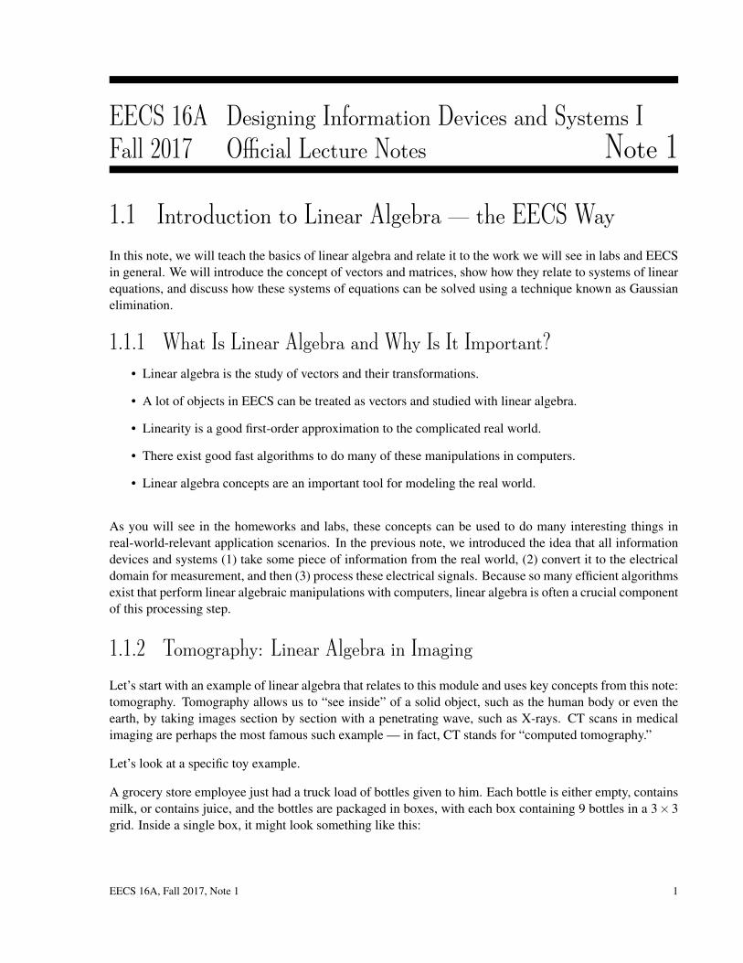
A grocery store employee just had a truck load of bottles given to him. Each bottle is either empty, containsmilk, or contains juice, and the bottles are packaged in boxes, with each box containing 9 bottles in a 3×3grid. Inside a single box, it might look something like this:

EECS 16A, Fall 2017, Note 1 1

If we choose symbols such that M=Milk, J=Juice, and O=Empty, we can represent the stack of bottles shownabove as follows:

M J OM J OM O J

(1)

Our grocer cannot see directly into the box, but he needs to sort them somehow (without opening everysingle one). However, suppose he has a device that can tell him how much light an object absorbs. This letshim shine a light at different angles to figure out how much total light the bottles in those columns absorb.

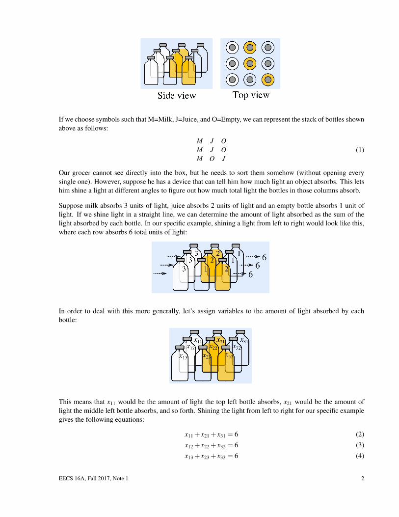
Suppose milk absorbs 3 units of light, juice absorbs 2 units of light and an empty bottle absorbs 1 unit oflight. If we shine light in a straight line, we can determine the amount of light absorbed as the sum of thelight absorbed by each bottle. In our specific example, shining a light from left to right would look like this,where each row absorbs 6 total units of light:

In order to deal with this more generally, let’s assign variables to the amount of light absorbed by eachbottle:

This means that x11 would be the amount of light the top left bottle absorbs, x21 would be the amount oflight the middle left bottle absorbs, and so forth. Shining the light from left to right for our specific examplegives the following equations:

x11 + x21 + x31 = 6 (2)

x12 + x22 + x32 = 6 (3)

x13 + x23 + x33 = 6 (4)


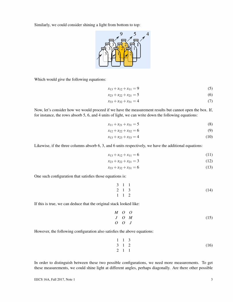
Similarly, we could consider shining a light from bottom to top:

Which would give the following equations:

x13 + x12 + x11 = 9 (5)

x23 + x22 + x21 = 5 (6)

x33 + x32 + x31 = 4 (7)

Now, let’s consider how we would proceed if we have the measurement results but cannot open the box. If,for instance, the rows absorb 5, 6, and 4 units of light, we can write down the following equations:

x11 + x21 + x31 = 5 (8)

x12 + x22 + x32 = 6 (9)

x13 + x23 + x33 = 4 (10)

Likewise, if the three columns absorb 6, 3, and 6 units respectively, we have the additional equations:

x13 + x12 + x11 = 6 (11)

x23 + x22 + x21 = 3 (12)

x33 + x32 + x31 = 6 (13)

One such configuration that satisfies those equations is:

3 1 12 1 31 1 2

(14)

If this is true, we can deduce that the original stack looked like:

M O OJ O MO O J

(15)

However, the following configuration also satisfies the above equations:

1 1 33 1 22 1 1

(16)

In order to distinguish between these two possible configurations, we need more measurements. To getthese measurements, we could shine light at different angles, perhaps diagonally. Are there other possible


configurations? How many different directions do we need to shine light through before we are certain ofthe configuration? By the end of this module, you will have the tools to answer these questions.

In lecture itself, we will work out specific examples to make this more clear. The important thing is that it isnot just about the number of measurements we take (or, equivalently, the number of experiments you do), butrather which measurements we take. These measurements must be chosen in a way that allows you to extractthe information that you are interested in. This doesn’t always happen. Sometimes, the measurements thatyou might think of taking end up being redundant in subtle ways.

1.2 Representing Systems of Linear EquationsIn our bottle-sorting tomography example, we represented each measurement in a row or column as anequation. The collection of equations is an example of a system of equations, which summarizes theknown relationships between the variables we want to solve for (x11,x12,x13, etc.) and our measurements.More specifically, the measurements in our tomography example can be characterized as a system of linearequations, because each variable relates to the measurement result by a fixed scaling factor.1 Because writingout all of these equations can be cumbersome, we will typically try to express systems of equations in termsof vectors and matrices instead. Here, we will briefly introduce the concepts of vectors and matrices inorder to illustrate how they can be used to represent systems of equations. In the next few lectures, we willgive you a bit more intuition and examples to demonstrate their role in science and engineering applications.

1.2.1 Vectors

Definition 1.1 (Vector): A vector is an ordered list of numbers. Suppose we have a collection of n realnumbers: x1,x2, · · · ,xn. This collection can be written as a single point in an n-dimensional space, denoted:

~x =

x1x2...

xn

. (17)

We call ~x a vector. Because ~x contains n real numbers, we can use the ∈ (“in” — i.e., is a member of)symbol to write ~x ∈ Rn. If the elements of ~x were complex numbers, we would write ~x ∈ Cn. Each xi (fori between 1 and n) is called a component, or element, of the vector. The size of a vector is the number ofcomponents it contains (n in the example vector, 2 in the example below).

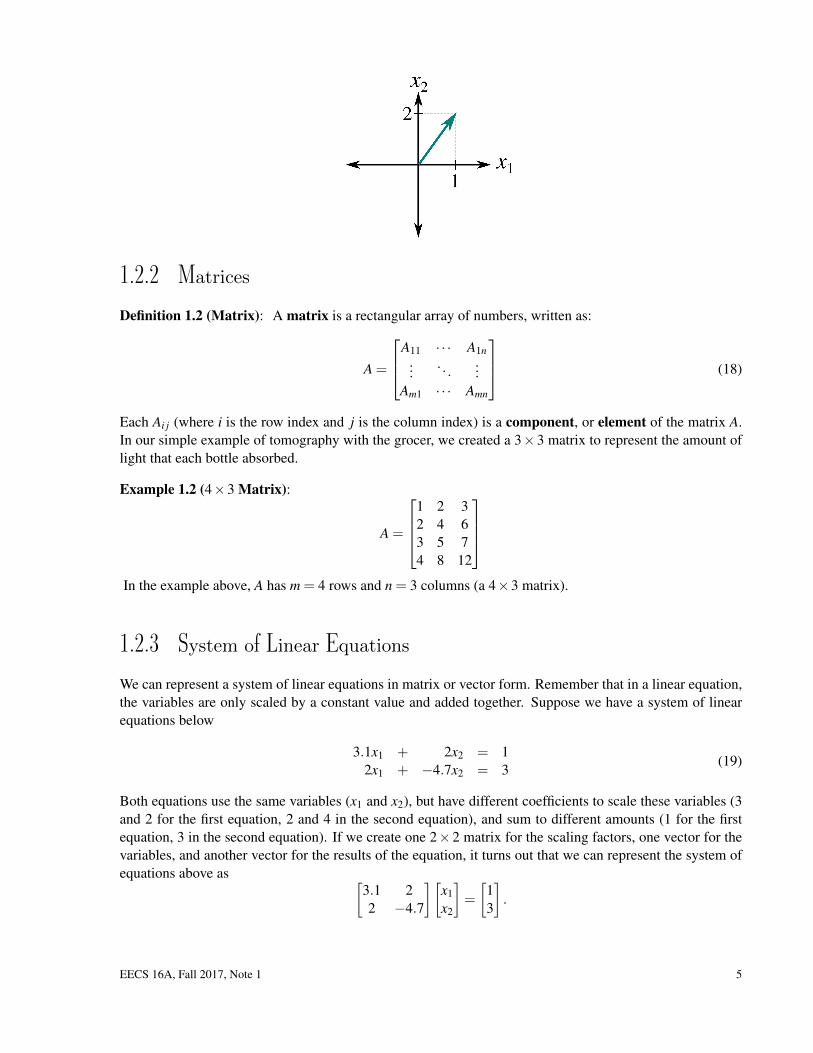
Example 1.1 (Vector of size 2):

~x =[

12

]In the above example,~x is a vector with two components. Because the components are both real numbers,~x ∈ R2. We can represent the vector graphically on a 2-D plane, using the first element, x1, to denote thehorizontal position of the vector and the second element, x2, to denote its vertical position:

1In the tomography example specifically, the scaling factor was either 1 or 0, but you could imagine different cases where thisscaling factor is any constant number. If you imagine plotting the measurement result as a function of each variable, you would geta line — hence the term “linear.”


1.2.2 Matrices

Definition 1.2 (Matrix): A matrix is a rectangular array of numbers, written as:

A =

A11 · · · A1n...

. . ....

Am1 · · · Amn

(18)

Each Ai j (where i is the row index and j is the column index) is a component, or element of the matrix A.In our simple example of tomography with the grocer, we created a 3×3 matrix to represent the amount oflight that each bottle absorbed.

Example 1.2 (4×3 Matrix):

A =

1 2 32 4 63 5 74 8 12

In the example above, A has m = 4 rows and n = 3 columns (a 4×3 matrix).

1.2.3 System of Linear Equations

We can represent a system of linear equations in matrix or vector form. Remember that in a linear equation,the variables are only scaled by a constant value and added together. Suppose we have a system of linearequations below

3.1x1 + 2x2 = 12x1 + −4.7x2 = 3

(19)

Both equations use the same variables (x1 and x2), but have different coefficients to scale these variables (3and 2 for the first equation, 2 and 4 in the second equation), and sum to different amounts (1 for the firstequation, 3 in the second equation). If we create one 2×2 matrix for the scaling factors, one vector for thevariables, and another vector for the results of the equation, it turns out that we can represent the system ofequations above as [

3.1 22 −4.7

][x1x2

]=

[13

].


In later notes, we will give more specifics about the details of matrix and vector multiplication, but ingeneral, we can represent any system of m linear equations with n variables in the form

A~x =~b

where A is an m×n matrix,~x is a vector containing the n variables, and~b is a vector of size m containing theconstants. Why do we care about writing a system of linear equations in the above representation? We willsee later in the course that decoupling the coefficients and the variables makes it easier to perform analysison the system, especially if the system is large.

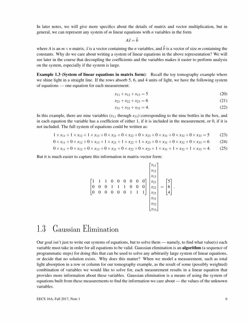
Example 1.3 (System of linear equations in matrix form): Recall the toy tomography example wherewe shine light in a straight line. If the rows absorb 5, 6, and 4 units of light, we have the following systemof equations — one equation for each measurement:

x11 + x12 + x13 = 5 (20)

x21 + x22 + x23 = 6 (21)

x31 + x32 + x33 = 4. (22)

In this example, there are nine variables (x11 through x33) corresponding to the nine bottles in the box, andin each equation the variable has a coefficient of either 1, if it is included in the measurement, or 0, if it isnot included. The full system of equations could be written as:

1× x11 +1× x12 +1× x13 +0× x21 +0× x22 +0× x23 +0× x31 +0× x32 +0× x33 = 5 (23)

0× x11 +0× x12 +0× x13 +1× x21 +1× x22 +1× x23 +0× x31 +0× x32 +0× x33 = 6 (24)

0× x11 +0× x12 +0× x13 +0× x21 +0× x22 +0× x23 +1× x31 +1× x32 +1× x33 = 4. (25)

But it is much easier to capture this information in matrix-vector form:

1 1 1 0 0 0 0 0 00 0 0 1 1 1 0 0 00 0 0 0 0 0 1 1 1

x11x12x13x21x22x23x31x32x33

=

564

.

1.3 Gaussian EliminationOur goal isn’t just to write out systems of equations, but to solve them — namely, to find what value(s) eachvariable must take in order for all equations to be valid. Gaussian elimination is an algorithm (a sequence ofprogrammatic steps) for doing this that can be used to solve any arbitrarily large system of linear equations,or decide that no solution exists. Why does this matter? When we model a measurement, such as totallight absorption in a row or column for our tomography example, as the result of some (possibly weighted)combination of variables we would like to solve for, each measurement results in a linear equation thatprovides more information about these variables. Gaussian elimination is a means of using the system ofequations built from these measurements to find the information we care about — the values of the unknownvariables.


1.3.1 Solving Systems of Linear Equations

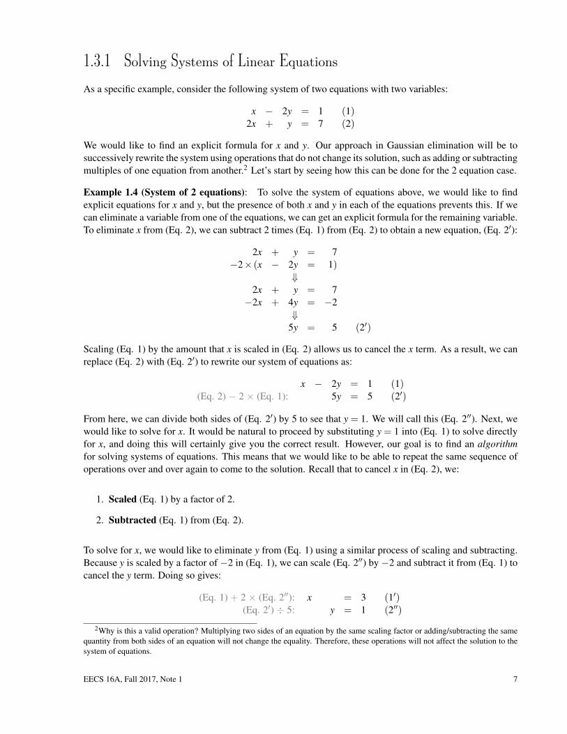
As a specific example, consider the following system of two equations with two variables:

x − 2y = 1 (1)2x + y = 7 (2)

We would like to find an explicit formula for x and y. Our approach in Gaussian elimination will be tosuccessively rewrite the system using operations that do not change its solution, such as adding or subtractingmultiples of one equation from another.2 Let’s start by seeing how this can be done for the 2 equation case.

Example 1.4 (System of 2 equations): To solve the system of equations above, we would like to findexplicit equations for x and y, but the presence of both x and y in each of the equations prevents this. If wecan eliminate a variable from one of the equations, we can get an explicit formula for the remaining variable.To eliminate x from (Eq. 2), we can subtract 2 times (Eq. 1) from (Eq. 2) to obtain a new equation, (Eq. 2′):

2x + y = 7−2× (x − 2y = 1)

⇓2x + y = 7−2x + 4y = −2

⇓5y = 5 (2′)

Scaling (Eq. 1) by the amount that x is scaled in (Eq. 2) allows us to cancel the x term. As a result, we canreplace (Eq. 2) with (Eq. 2′) to rewrite our system of equations as:

x − 2y = 1 (1)(Eq. 2) − 2 × (Eq. 1): 5y = 5 (2′)

From here, we can divide both sides of (Eq. 2′) by 5 to see that y = 1. We will call this (Eq. 2′′). Next, wewould like to solve for x. It would be natural to proceed by substituting y = 1 into (Eq. 1) to solve directlyfor x, and doing this will certainly give you the correct result. However, our goal is to find an algorithmfor solving systems of equations. This means that we would like to be able to repeat the same sequence ofoperations over and over again to come to the solution. Recall that to cancel x in (Eq. 2), we:

1. Scaled (Eq. 1) by a factor of 2.

2. Subtracted (Eq. 1) from (Eq. 2).

To solve for x, we would like to eliminate y from (Eq. 1) using a similar process of scaling and subtracting.Because y is scaled by a factor of −2 in (Eq. 1), we can scale (Eq. 2′′) by −2 and subtract it from (Eq. 1) tocancel the y term. Doing so gives:

(Eq. 1) + 2 × (Eq. 2′′): x = 3 (1′)(Eq. 2′) ÷ 5: y = 1 (2′′)

2Why is this a valid operation? Multiplying two sides of an equation by the same scaling factor or adding/subtracting the samequantity from both sides of an equation will not change the equality. Therefore, these operations will not affect the solution to thesystem of equations.


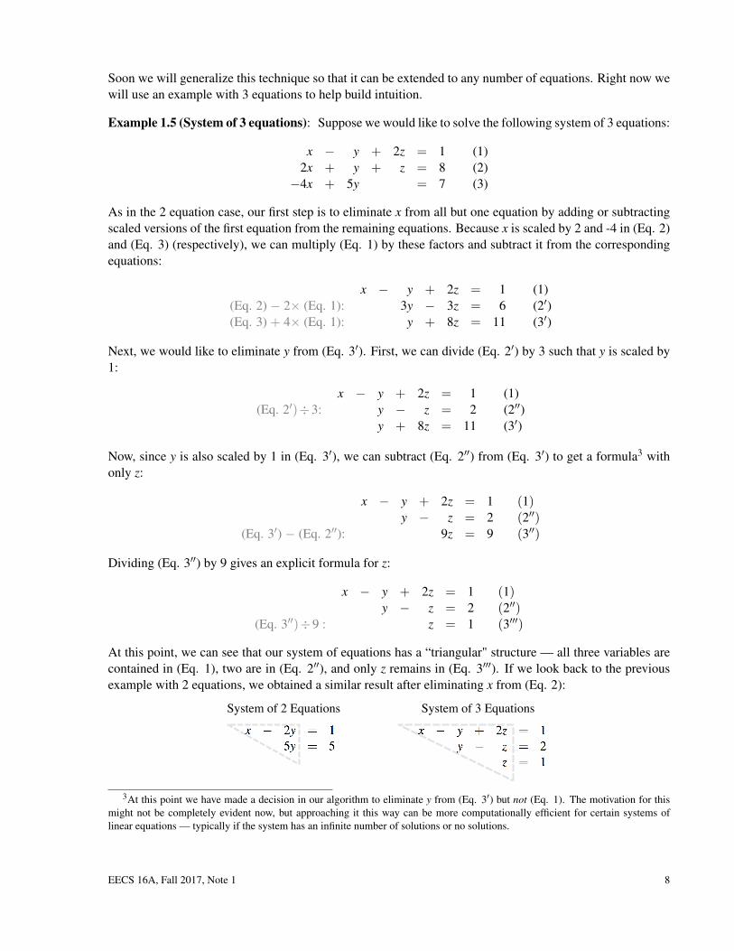
Soon we will generalize this technique so that it can be extended to any number of equations. Right now wewill use an example with 3 equations to help build intuition.

Example 1.5 (System of 3 equations): Suppose we would like to solve the following system of 3 equations:

x − y + 2z = 1 (1)2x + y + z = 8 (2)−4x + 5y = 7 (3)

As in the 2 equation case, our first step is to eliminate x from all but one equation by adding or subtractingscaled versions of the first equation from the remaining equations. Because x is scaled by 2 and -4 in (Eq. 2)and (Eq. 3) (respectively), we can multiply (Eq. 1) by these factors and subtract it from the correspondingequations:

x − y + 2z = 1 (1)(Eq. 2) − 2× (Eq. 1): 3y − 3z = 6 (2′)(Eq. 3) + 4× (Eq. 1): y + 8z = 11 (3′)

Next, we would like to eliminate y from (Eq. 3′). First, we can divide (Eq. 2′) by 3 such that y is scaled by1:

x − y + 2z = 1 (1)(Eq. 2′)÷3: y − z = 2 (2′′)

y + 8z = 11 (3′)

Now, since y is also scaled by 1 in (Eq. 3′), we can subtract (Eq. 2′′) from (Eq. 3′) to get a formula3 withonly z:

x − y + 2z = 1 (1)y − z = 2 (2′′)

(Eq. 3′) − (Eq. 2′′): 9z = 9 (3′′)

Dividing (Eq. 3′′) by 9 gives an explicit formula for z:

x − y + 2z = 1 (1)y − z = 2 (2′′)

(Eq. 3′′)÷9 : z = 1 (3′′′)

At this point, we can see that our system of equations has a “triangular" structure — all three variables arecontained in (Eq. 1), two are in (Eq. 2′′), and only z remains in (Eq. 3′′′). If we look back to the previousexample with 2 equations, we obtained a similar result after eliminating x from (Eq. 2):

System of 2 Equations System of 3 Equations

3At this point we have made a decision in our algorithm to eliminate y from (Eq. 3′) but not (Eq. 1). The motivation for thismight not be completely evident now, but approaching it this way can be more computationally efficient for certain systems oflinear equations — typically if the system has an infinite number of solutions or no solutions.


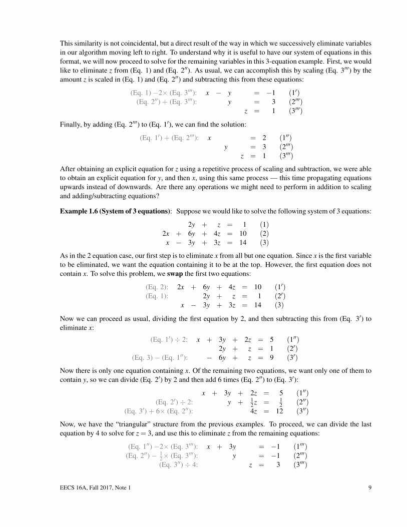
This similarity is not coincidental, but a direct result of the way in which we successively eliminate variablesin our algorithm moving left to right. To understand why it is useful to have our system of equations in thisformat, we will now proceed to solve for the remaining variables in this 3-equation example. First, we wouldlike to eliminate z from (Eq. 1) and (Eq. 2′′). As usual, we can accomplish this by scaling (Eq. 3′′′) by theamount z is scaled in (Eq. 1) and (Eq. 2′′) and subtracting this from these equations:

(Eq. 1) −2× (Eq. 3′′′): x − y = −1 (1′)(Eq. 2′′) + (Eq. 3′′′): y = 3 (2′′′)

z = 1 (3′′′)

Finally, by adding (Eq. 2′′′) to (Eq. 1′), we can find the solution:

(Eq. 1′) + (Eq. 2′′′): x = 2 (1′′)y = 3 (2′′′)

z = 1 (3′′′)

After obtaining an explicit equation for z using a repetitive process of scaling and subtraction, we were ableto obtain an explicit equation for y, and then x, using this same process — this time propagating equationsupwards instead of downwards. Are there any operations we might need to perform in addition to scalingand adding/subtracting equations?

Example 1.6 (System of 3 equations): Suppose we would like to solve the following system of 3 equations:

2y + z = 1 (1)2x + 6y + 4z = 10 (2)x − 3y + 3z = 14 (3)

As in the 2 equation case, our first step is to eliminate x from all but one equation. Since x is the first variableto be eliminated, we want the equation containing it to be at the top. However, the first equation does notcontain x. To solve this problem, we swap the first two equations:

(Eq. 2): 2x + 6y + 4z = 10 (1′)(Eq. 1): 2y + z = 1 (2′)

x − 3y + 3z = 14 (3)

Now we can proceed as usual, dividing the first equation by 2, and then subtracting this from (Eq. 3′) toeliminate x:

(Eq. 1′) ÷ 2: x + 3y + 2z = 5 (1′′)2y + z = 1 (2′)

(Eq. 3) − (Eq. 1′′): − 6y + z = 9 (3′)

Now there is only one equation containing x. Of the remaining two equations, we want only one of them tocontain y, so we can divide (Eq. 2′) by 2 and then add 6 times (Eq. 2′′) to (Eq. 3′):

x + 3y + 2z = 5 (1′′)(Eq. 2′) ÷ 2: y + 1

2 z = 12 (2′′)

(Eq. 3′) + 6× (Eq. 2′′): 4z = 12 (3′′)

Now, we have the “triangular” structure from the previous examples. To proceed, we can divide the lastequation by 4 to solve for z = 3, and use this to eliminate z from the remaining equations:

(Eq. 1′′) −2× (Eq. 3′′′): x + 3y = −1 (1′′′)(Eq. 2′′) − 1

2× (Eq. 3′′′): y = −1 (2′′′)(Eq. 3′′) ÷ 4: z = 3 (3′′′)


Finally, we can subtract 3 times (Eq. 2′′′) from (Eq. 1′′′) to solve for x:

(Eq. 1′′′) −3× (Eq. 2′′′): x = 2 (1′′′′)y = −1 (2′′′)

z = 3 (3′′′)

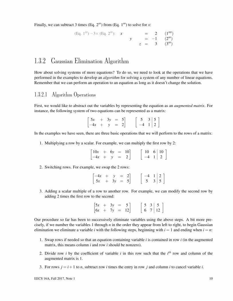
1.3.2 Gaussian Elimination AlgorithmHow about solving systems of more equations? To do so, we need to look at the operations that we haveperformed in the examples to develop an algorithm for solving a system of any number of linear equations.Remember that we can perform an operation to an equation as long as it doesn’t change the solution.

1.3.2.1 Algorithm Operations

First, we would like to abstract out the variables by representing the equation as an augmented matrix. Forinstance, the following system of two equations can be represented as a matrix:[

5x + 3y = 5−4x + y = 2

] [5 3 5−4 1 2

]In the examples we have seen, there are three basic operations that we will perform to the rows of a matrix:

1. Multiplying a row by a scalar. For example, we can multiply the first row by 2:[10x + 6y = 10−4x + y = 2

] [10 6 10−4 1 2

]2. Switching rows. For example, we swap the 2 rows:[

−4x + y = 25x + 3y = 5

] [−4 1 25 3 5

]3. Adding a scalar multiple of a row to another row. For example, we can modify the second row by

adding 2 times the first row to the second:[5x + 3y = 56x + 7y = 12

] [5 3 56 7 12

]Our procedure so far has been to successively eliminate variables using the above steps. A bit more pre-cisely, if we number the variables 1 through n in the order they appear from left to right, to begin Gaussianelimination we eliminate a variable i with the following steps, beginning with i = 1 and ending when i = n:

1. Swap rows if needed so that an equation containing variable i is contained in row i (in the augmentedmatrix, this means column i and row i should be nonzero).

2. Divide row i by the coefficient of variable i in this row such that the ith row and column of theaugmented matrix is 1.

3. For rows j = i+1 to n, subtract row i times the entry in row j and column i to cancel variable i.


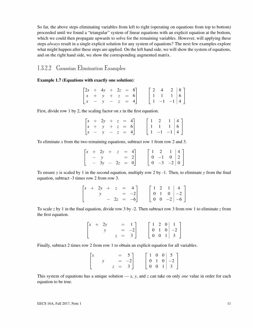
So far, the above steps eliminating variables from left to right (operating on equations from top to bottom)proceeded until we found a “triangular” system of linear equations with an explicit equation at the bottom,which we could then propagate upwards to solve for the remaining variables. However, will applying thesesteps always result in a single explicit solution for any system of equations? The next few examples explorewhat might happen after these steps are applied. On the left hand side, we will show the system of equations,and on the right hand side, we show the corresponding augmented matrix.

1.3.2.2 Gaussian Elimination Examples

Example 1.7 (Equations with exactly one solution):2x + 4y + 2z = 8x + y + z = 6x − y − z = 4

2 4 2 81 1 1 61 −1 −1 4

First, divide row 1 by 2, the scaling factor on x in the first equation.x + 2y + z = 4

x + y + z = 6x − y − z = 4

1 2 1 41 1 1 61 −1 −1 4

To eliminate x from the two remaining equations, subtract row 1 from row 2 and 3.x + 2y + z = 4

− y = 2− 3y − 2z = 0

1 2 1 40 −1 0 20 −3 −2 0

To ensure y is scaled by 1 in the second equation, multiply row 2 by -1. Then, to eliminate y from the finalequation, subtract -3 times row 2 from row 3.x + 2y + z = 4

y = −2− 2z = −6

1 2 1 40 1 0 −20 0 −2 −6

To scale z by 1 in the final equation, divide row 3 by -2. Then subtract row 3 from row 1 to eliminate z fromthe first equation. x + 2y = 1

y = −2z = 3

1 2 0 10 1 0 −20 0 1 3

Finally, subtract 2 times row 2 from row 1 to obtain an explicit equation for all variables.x = 5

y = −2z = 3

1 0 0 50 1 0 −20 0 1 3

This system of equations has a unique solution — x, y, and z can take on only one value in order for eachequation to be true.


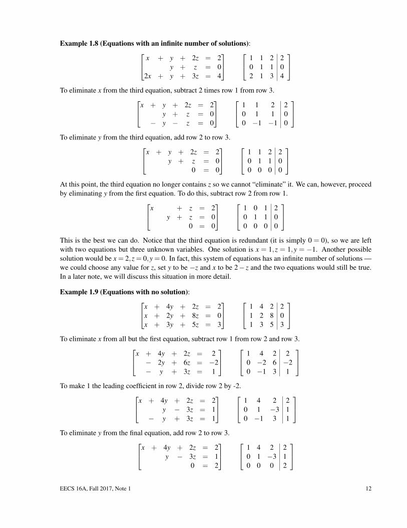
Example 1.8 (Equations with an infinite number of solutions): x + y + 2z = 2y + z = 0

2x + y + 3z = 4

1 1 2 20 1 1 02 1 3 4

To eliminate x from the third equation, subtract 2 times row 1 from row 3.x + y + 2z = 2

y + z = 0− y − z = 0

1 1 2 20 1 1 00 −1 −1 0

To eliminate y from the third equation, add row 2 to row 3.x + y + 2z = 2

y + z = 00 = 0

1 1 2 20 1 1 00 0 0 0

At this point, the third equation no longer contains z so we cannot “eliminate” it. We can, however, proceedby eliminating y from the first equation. To do this, subtract row 2 from row 1.x + z = 2

y + z = 00 = 0

1 0 1 20 1 1 00 0 0 0

This is the best we can do. Notice that the third equation is redundant (it is simply 0 = 0), so we are leftwith two equations but three unknown variables. One solution is x = 1,z = 1,y = −1. Another possiblesolution would be x = 2,z = 0,y = 0. In fact, this system of equations has an infinite number of solutions —we could choose any value for z, set y to be −z and x to be 2− z and the two equations would still be true.In a later note, we will discuss this situation in more detail.

Example 1.9 (Equations with no solution):x + 4y + 2z = 2x + 2y + 8z = 0x + 3y + 5z = 3

1 4 2 21 2 8 01 3 5 3

To eliminate x from all but the first equation, subtract row 1 from row 2 and row 3.x + 4y + 2z = 2

− 2y + 6z = −2− y + 3z = 1

1 4 2 20 −2 6 −20 −1 3 1

To make 1 the leading coefficient in row 2, divide row 2 by -2.x + 4y + 2z = 2

y − 3z = 1− y + 3z = 1

1 4 2 20 1 −3 10 −1 3 1

To eliminate y from the final equation, add row 2 to row 3.x + 4y + 2z = 2

y − 3z = 10 = 2

1 4 2 20 1 −3 10 0 0 2


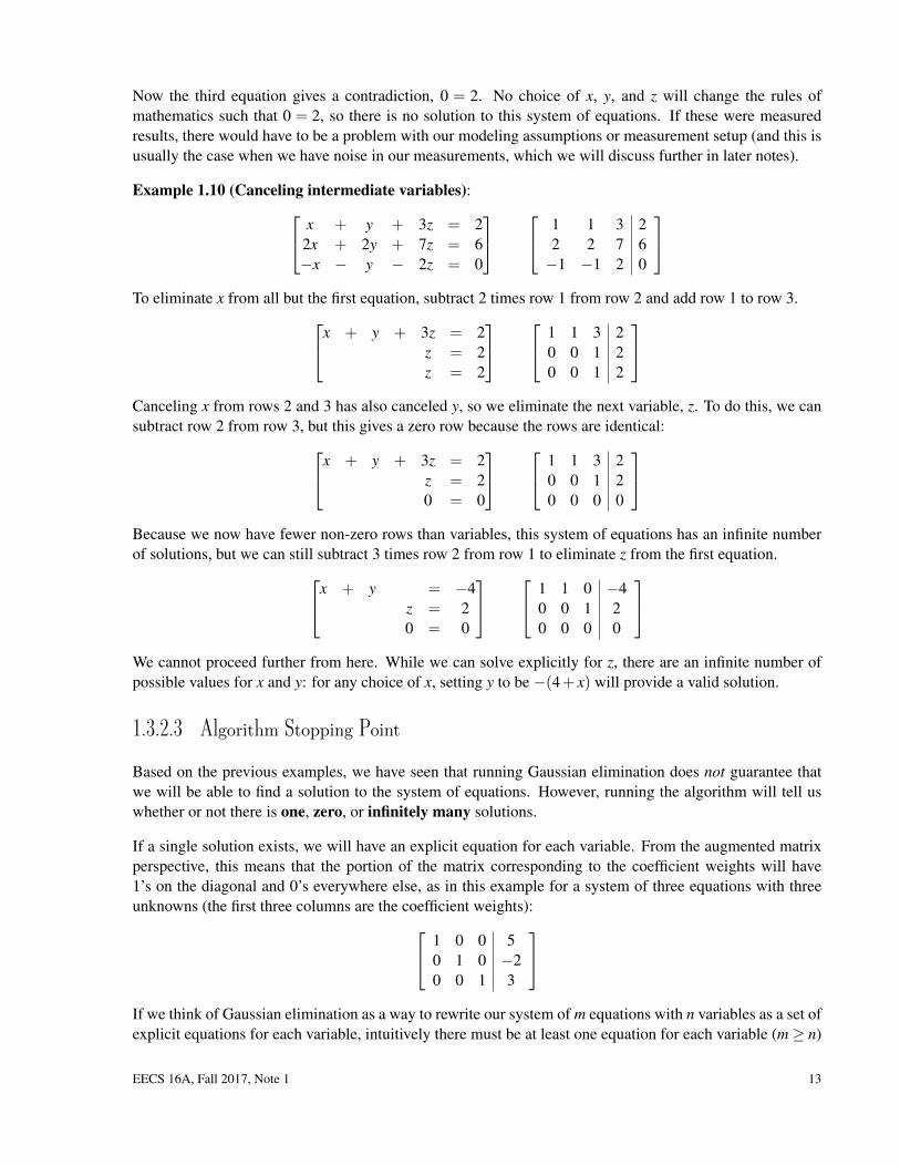
Now the third equation gives a contradiction, 0 = 2. No choice of x, y, and z will change the rules ofmathematics such that 0 = 2, so there is no solution to this system of equations. If these were measuredresults, there would have to be a problem with our modeling assumptions or measurement setup (and this isusually the case when we have noise in our measurements, which we will discuss further in later notes).

Example 1.10 (Canceling intermediate variables): x + y + 3z = 22x + 2y + 7z = 6−x − y − 2z = 0

1 1 3 22 2 7 6−1 −1 2 0

To eliminate x from all but the first equation, subtract 2 times row 1 from row 2 and add row 1 to row 3.x + y + 3z = 2

z = 2z = 2

1 1 3 20 0 1 20 0 1 2

Canceling x from rows 2 and 3 has also canceled y, so we eliminate the next variable, z. To do this, we cansubtract row 2 from row 3, but this gives a zero row because the rows are identical:x + y + 3z = 2

z = 20 = 0

1 1 3 20 0 1 20 0 0 0

Because we now have fewer non-zero rows than variables, this system of equations has an infinite numberof solutions, but we can still subtract 3 times row 2 from row 1 to eliminate z from the first equation.x + y = −4

z = 20 = 0

1 1 0 −40 0 1 20 0 0 0

We cannot proceed further from here. While we can solve explicitly for z, there are an infinite number ofpossible values for x and y: for any choice of x, setting y to be −(4+ x) will provide a valid solution.

1.3.2.3 Algorithm Stopping Point

Based on the previous examples, we have seen that running Gaussian elimination does not guarantee thatwe will be able to find a solution to the system of equations. However, running the algorithm will tell uswhether or not there is one, zero, or infinitely many solutions.

If a single solution exists, we will have an explicit equation for each variable. From the augmented matrixperspective, this means that the portion of the matrix corresponding to the coefficient weights will have1’s on the diagonal and 0’s everywhere else, as in this example for a system of three equations with threeunknowns (the first three columns are the coefficient weights): 1 0 0 5

0 1 0 −20 0 1 3

If we think of Gaussian elimination as a way to rewrite our system of m equations with n variables as a set ofexplicit equations for each variable, intuitively there must be at least one equation for each variable (m≥ n)


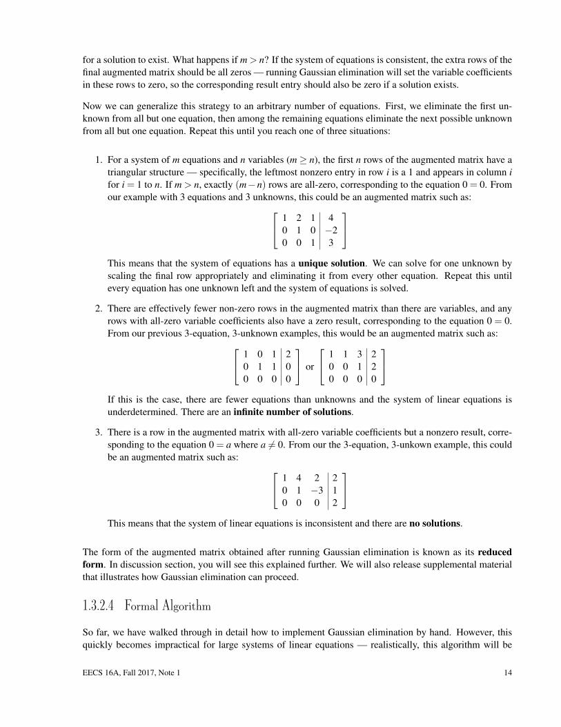
for a solution to exist. What happens if m > n? If the system of equations is consistent, the extra rows of thefinal augmented matrix should be all zeros — running Gaussian elimination will set the variable coefficientsin these rows to zero, so the corresponding result entry should also be zero if a solution exists.

Now we can generalize this strategy to an arbitrary number of equations. First, we eliminate the first un-known from all but one equation, then among the remaining equations eliminate the next possible unknownfrom all but one equation. Repeat this until you reach one of three situations:

1. For a system of m equations and n variables (m≥ n), the first n rows of the augmented matrix have atriangular structure — specifically, the leftmost nonzero entry in row i is a 1 and appears in column ifor i = 1 to n. If m > n, exactly (m−n) rows are all-zero, corresponding to the equation 0 = 0. Fromour example with 3 equations and 3 unknowns, this could be an augmented matrix such as: 1 2 1 4

0 1 0 −20 0 1 3

This means that the system of equations has a unique solution. We can solve for one unknown byscaling the final row appropriately and eliminating it from every other equation. Repeat this untilevery equation has one unknown left and the system of equations is solved.

2. There are effectively fewer non-zero rows in the augmented matrix than there are variables, and anyrows with all-zero variable coefficients also have a zero result, corresponding to the equation 0 = 0.From our previous 3-equation, 3-unknown examples, this would be an augmented matrix such as: 1 0 1 2

0 1 1 00 0 0 0

or

1 1 3 20 0 1 20 0 0 0

If this is the case, there are fewer equations than unknowns and the system of linear equations isunderdetermined. There are an infinite number of solutions.

3. There is a row in the augmented matrix with all-zero variable coefficients but a nonzero result, corre-sponding to the equation 0 = a where a 6= 0. From our the 3-equation, 3-unkown example, this couldbe an augmented matrix such as: 1 4 2 2

0 1 −3 10 0 0 2

This means that the system of linear equations is inconsistent and there are no solutions.

The form of the augmented matrix obtained after running Gaussian elimination is known as its reducedform. In discussion section, you will see this explained further. We will also release supplemental materialthat illustrates how Gaussian elimination can proceed.

1.3.2.4 Formal Algorithm

So far, we have walked through in detail how to implement Gaussian elimination by hand. However, thisquickly becomes impractical for large systems of linear equations — realistically, this algorithm will be


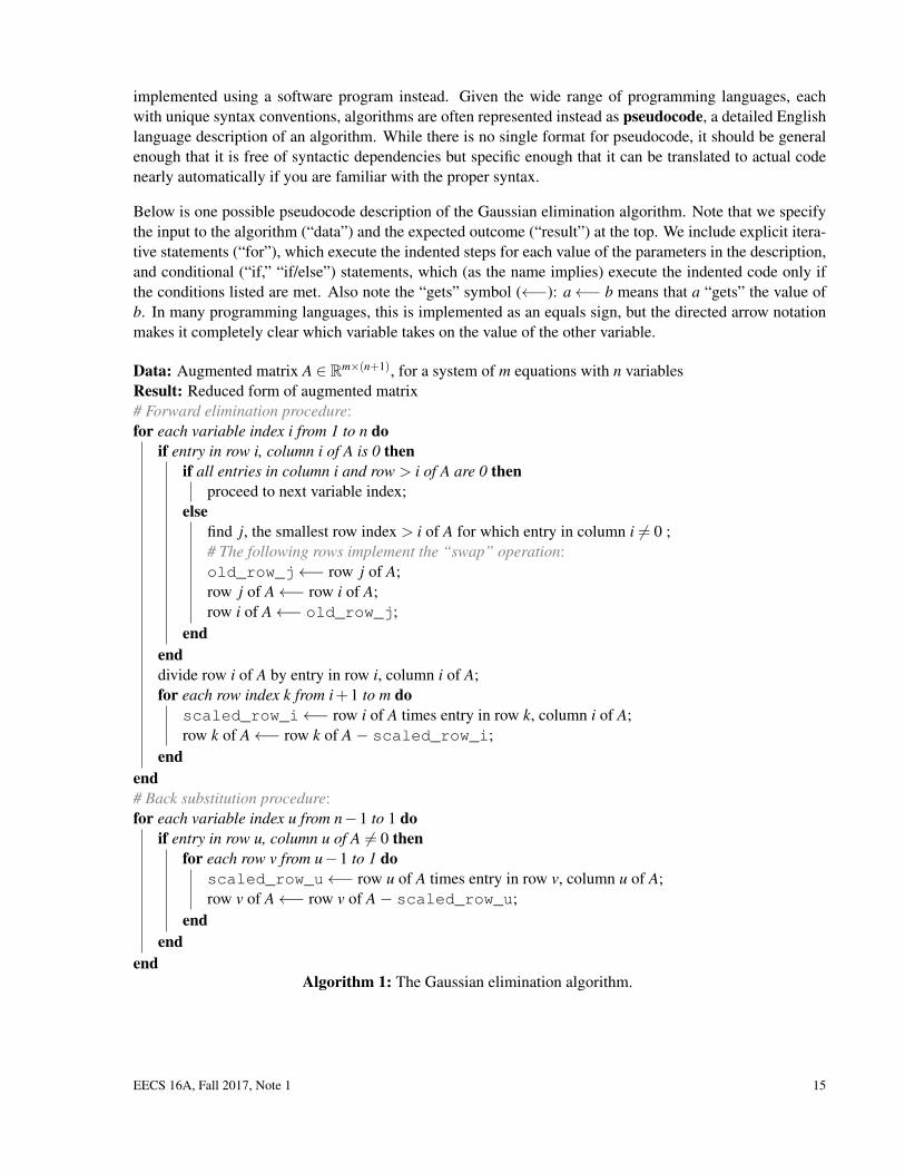
implemented using a software program instead. Given the wide range of programming languages, eachwith unique syntax conventions, algorithms are often represented instead as pseudocode, a detailed Englishlanguage description of an algorithm. While there is no single format for pseudocode, it should be generalenough that it is free of syntactic dependencies but specific enough that it can be translated to actual codenearly automatically if you are familiar with the proper syntax.

Below is one possible pseudocode description of the Gaussian elimination algorithm. Note that we specifythe input to the algorithm (“data”) and the expected outcome (“result”) at the top. We include explicit itera-tive statements (“for”), which execute the indented steps for each value of the parameters in the description,and conditional (“if,” “if/else”) statements, which (as the name implies) execute the indented code only ifthe conditions listed are met. Also note the “gets” symbol (←−): a←− b means that a “gets” the value ofb. In many programming languages, this is implemented as an equals sign, but the directed arrow notationmakes it completely clear which variable takes on the value of the other variable.

Data: Augmented matrix A ∈ Rm×(n+1), for a system of m equations with n variablesResult: Reduced form of augmented matrix# Forward elimination procedure:for each variable index i from 1 to n do

if entry in row i, column i of A is 0 thenif all entries in column i and row > i of A are 0 then

proceed to next variable index;else

find j, the smallest row index > i of A for which entry in column i 6= 0 ;# The following rows implement the “swap” operation:old_row_j←− row j of A;row j of A←− row i of A;row i of A←− old_row_j;

endenddivide row i of A by entry in row i, column i of A;for each row index k from i+1 to m do

scaled_row_i←− row i of A times entry in row k, column i of A;row k of A←− row k of A − scaled_row_i;

endend# Back substitution procedure:for each variable index u from n−1 to 1 do

if entry in row u, column u of A 6= 0 thenfor each row v from u−1 to 1 do

scaled_row_u←− row u of A times entry in row v, column u of A;row v of A←− row v of A − scaled_row_u;

endend

endAlgorithm 1: The Gaussian elimination algorithm.


1.3.3 Tomography Revisited

How does what we have learned so far relate back to our tomography example? We know that becauseour grocer’s measurements come from a specific box with a particular assortment of milk, juice, and emptybottles, there must be one underlying solution, but insufficient measurements could give us a system ofequations with an infinite number of solutions. So, how many measurements do we need?

Initially, we thought about shining a light vertically and horizontally through the box, giving six total equa-tions because there are three rows and three columns per box. However, there are nine bottles to identify, andtherefore nine variables, so we will need nine equations. Based on what you have learned about Gaussianelimination, you now understand that we need at least three more measurements — likely taken diagonally— in order to properly identify the bottles. In coming notes, we will discuss in further detail how you cantell whether or not the nine measurements you choose will allow you to find the solution.


eecs 16a designing information devices and systems i fall 2017 o cial lecture...

Documents