Effects of Airfoil Geometry and Mechanical

Characteristics on the Onset of Flutter

(As a Basis for Future Work on the Effects of

Structural Polynomial Nonlinearities on the Flutter

Boundary)

Udbhav Sharma

gte271u@mail.gatech.edu

School of Aerospace Engineering

Georgia Institute of Technology

December 10, 2004

Abstract

This paper derives linear 2nd order ordinary differential equations describ-

ing the motion of a 2 dimensional airfoil allowing for 3 spatial Degrees of

Freedom in airfoil angular rotation, vertical movement and control surface

rotation. The equations of motion are derived from a conservative Euler-

Lagrange formulation with the non-dissipative forcing functions arising from

steady, incompressible, inviscid 2 dimensional aerodynamics incorporating

results from Thin Airfoil Theory. The resulting model predicts undamped,

increasing oscillations below a critical airflow speed called the flutter bound-

ary. The paper shows how this speed can be predicted from the eigenvalues

of the system. By changing certain airfoil geometrical and mechanical prop-

erties, it is demonstrated that it is possible to aeroelastically tailor the airfoil

such that flutter is avoided for a given flight regime. The model adopted

has been found deficient in its ability to predict a realistic flutter boundary.

This problem is due to the absence of dissipative forces in the aerodynam-

ics of the model. It has been suggested that the model can be made more

realistic by incorporating unsteadiness into the aerodynamics of the system

using results from Peters’ finite state theory.

1 Introduction

Aeroelasticity studies the dynamics of an elastic body moving through a

fluid and undergoing deformation due to aerodynamic forces. Aeroelastic

considerations are of vital importance in the design of aerospacecraft be-

cause vibration in lifting surfaces, called flutter, can lead to structural fa-

tigue and even catastrophic failure [1]. An important problem concerns the

prediction and characterization of the so called flutter boundary (or speed)

in aircraft wings. Classical aeroelastic theories [2] predict damped expo-

nentially decreasing oscillations for an aircraft surface perturbed at speeds

below the critical flutter boundary. However, exponentially increasing os-

cillations are predicted beyond this speed [3]. Therefore, knowledge of the

stability boundary is vital to avoid hazardous flight regimes. This stabil-

ity problem is studied in classical theories with the governing equations of

motion reduced to a set of linear ordinary differential equations [2].

Linear aeroelastic models fail to capture the dynamics of the system in

the vicinity of the flutter boundary. Stable limit cycle oscillations (LCO)

have been observed in wind tunnel models [3] and real aircraft [1] at speeds

in the neighborhood of the predicted flutter boundary. These so called ”be-

nign”, finite amplitude, steady state oscillations are unfortunately not the

only possible effect. Unstable LCO have also been noticed both before and

after the onset of the predicted flutter speed [3]. In the case of unstable

LCO, the oscillations grow suddenly to very large amplitudes causing catas-

trophic flutter and structural failure. A more accurate aeroelastic model

will need to incorporate nonlinearities present in the system to account for

such phenomena.

Nonlinear effects in aeroelasticity arise from either the aerodynamics of

1

the flow or from the elastic structure of the airfoil [3]. Sources of nonlinearity

in aerodynamics include the presence of shocks in transonic and supersonic

flow regimes and large angle of attack effects, where the flow becomes sep-

arated from the airfoil surface [3]. Structural nonlinearities are known to

arise from freeplay or slop in the control surfaces, friction between moving

parts and continuous nonlinearities in structural stiffness [3].

This paper is the first step in developing a structurally nonlinear aeroe-

lastic model with unsteady aerodynamics. We first adopt a linear aerody-

namic model that limits the ambient airflow to inviscid, incompressible (low

Mach number) and steady state flow. A more sophisticated unsteady aero-

dynamic model such as Peters’ finite-state Thin Airfoil Theory will be re-

quired to capture dissipative effects in flutter. Since we derive the structural

equations separately from the aerodynamics, it will be simple to adopt more

sophisticated aerodynamics at a later stage without affecting the structural

model. Further development will include the addition of nonlinear polyno-

mial terms to model structural stiffness coefficients once the unsteady model

is in place.

2 Equations of motion

The aeroelastic behavior of aircraft lifting surfaces has traditionally been

studied with a simple 2 dimensional (2D) typical airfoil section model [2].

An airfoil section (or airfoil) is physically a cross section of a wing or other

lifting surface. The flow around this section is assumed to be representa-

tive of the flow around the wing. Since the airfoil section is modeled as a

rigid body, elastic deformations due to structural bending and torsion are

modeled by springs attached to the airfoil [1]. The use of an airfoil model

2

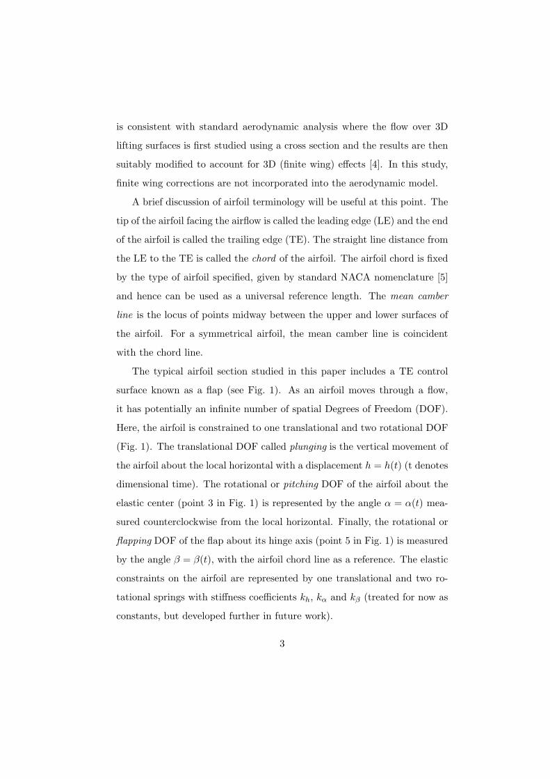
is consistent with standard aerodynamic analysis where the flow over 3D

lifting surfaces is first studied using a cross section and the results are then

suitably modified to account for 3D (finite wing) effects [4]. In this study,

finite wing corrections are not incorporated into the aerodynamic model.

A brief discussion of airfoil terminology will be useful at this point. The

tip of the airfoil facing the airflow is called the leading edge (LE) and the end

of the airfoil is called the trailing edge (TE). The straight line distance from

the LE to the TE is called the chord of the airfoil. The airfoil chord is fixed

by the type of airfoil specified, given by standard NACA nomenclature [5]

and hence can be used as a universal reference length. The mean camber

line is the locus of points midway between the upper and lower surfaces of

the airfoil. For a symmetrical airfoil, the mean camber line is coincident

with the chord line.

The typical airfoil section studied in this paper includes a TE control

surface known as a flap (see Fig. 1). As an airfoil moves through a flow,

it has potentially an infinite number of spatial Degrees of Freedom (DOF).

Here, the airfoil is constrained to one translational and two rotational DOF

(Fig. 1). The translational DOF called plunging is the vertical movement of

the airfoil about the local horizontal with a displacement h = h(t) (t denotes

dimensional time). The rotational or pitching DOF of the airfoil about the

elastic center (point 3 in Fig. 1) is represented by the angle α = α(t) mea-

sured counterclockwise from the local horizontal. Finally, the rotational or

flapping DOF of the flap about its hinge axis (point 5 in Fig. 1) is measured

by the angle β = β(t), with the airfoil chord line as a reference. The elastic

constraints on the airfoil are represented by one translational and two ro-

tational springs with stiffness coefficients kh, kα and kβ (treated for now as

constants, but developed further in future work).

3

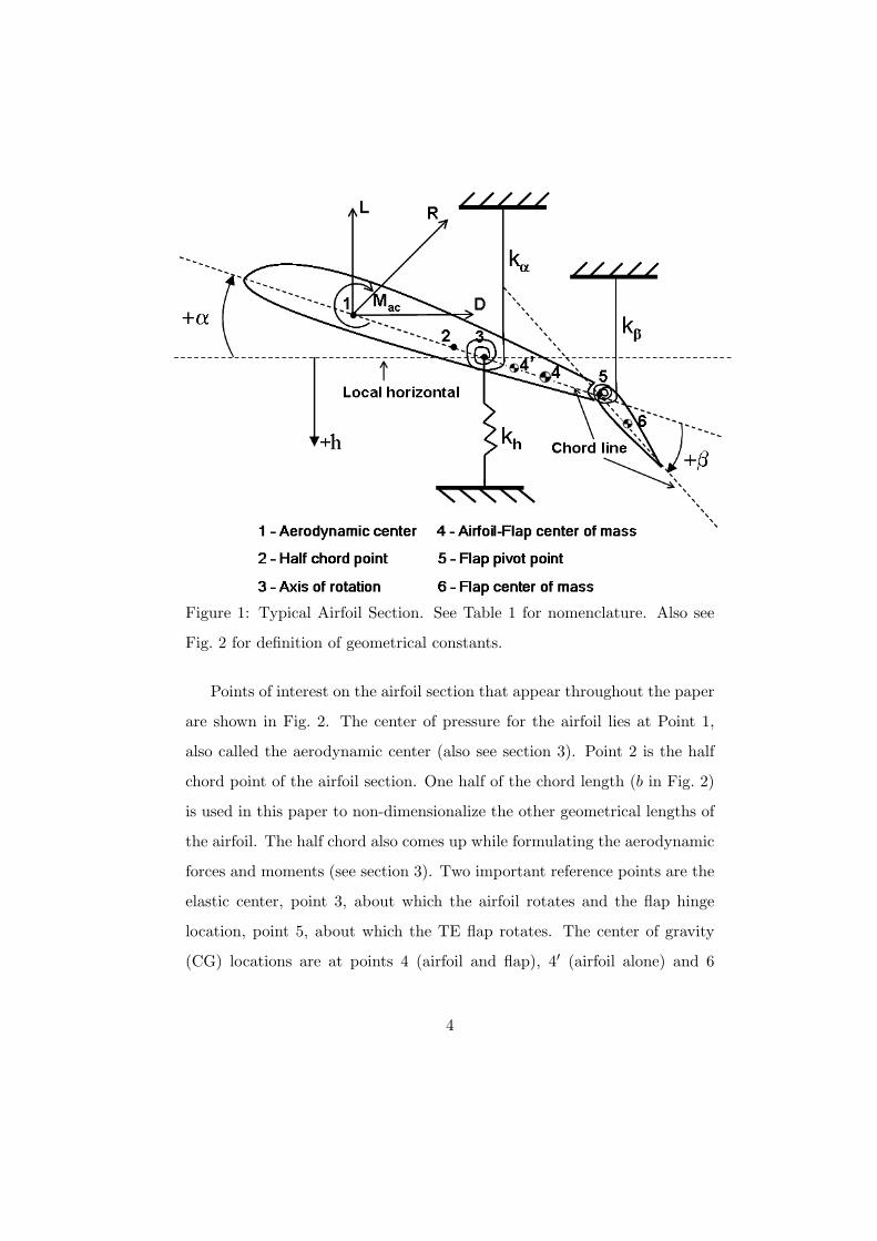
Figure 1: Typical Airfoil Section. See Table 1 for nomenclature. Also see

Fig. 2 for definition of geometrical constants.

Points of interest on the airfoil section that appear throughout the paper

are shown in Fig. 2. The center of pressure for the airfoil lies at Point 1,

also called the aerodynamic center (also see section 3). Point 2 is the half

chord point of the airfoil section. One half of the chord length (b in Fig. 2)

is used in this paper to non-dimensionalize the other geometrical lengths of

the airfoil. The half chord also comes up while formulating the aerodynamic

forces and moments (see section 3). Two important reference points are the

elastic center, point 3, about which the airfoil rotates and the flap hinge

location, point 5, about which the TE flap rotates. The center of gravity

(CG) locations are at points 4 (airfoil and flap), 4′ (airfoil alone) and 6

4

(flap alone). The geometrical constants relating these points are defined

graphically in Fig. 2 and summarized in Table 1.

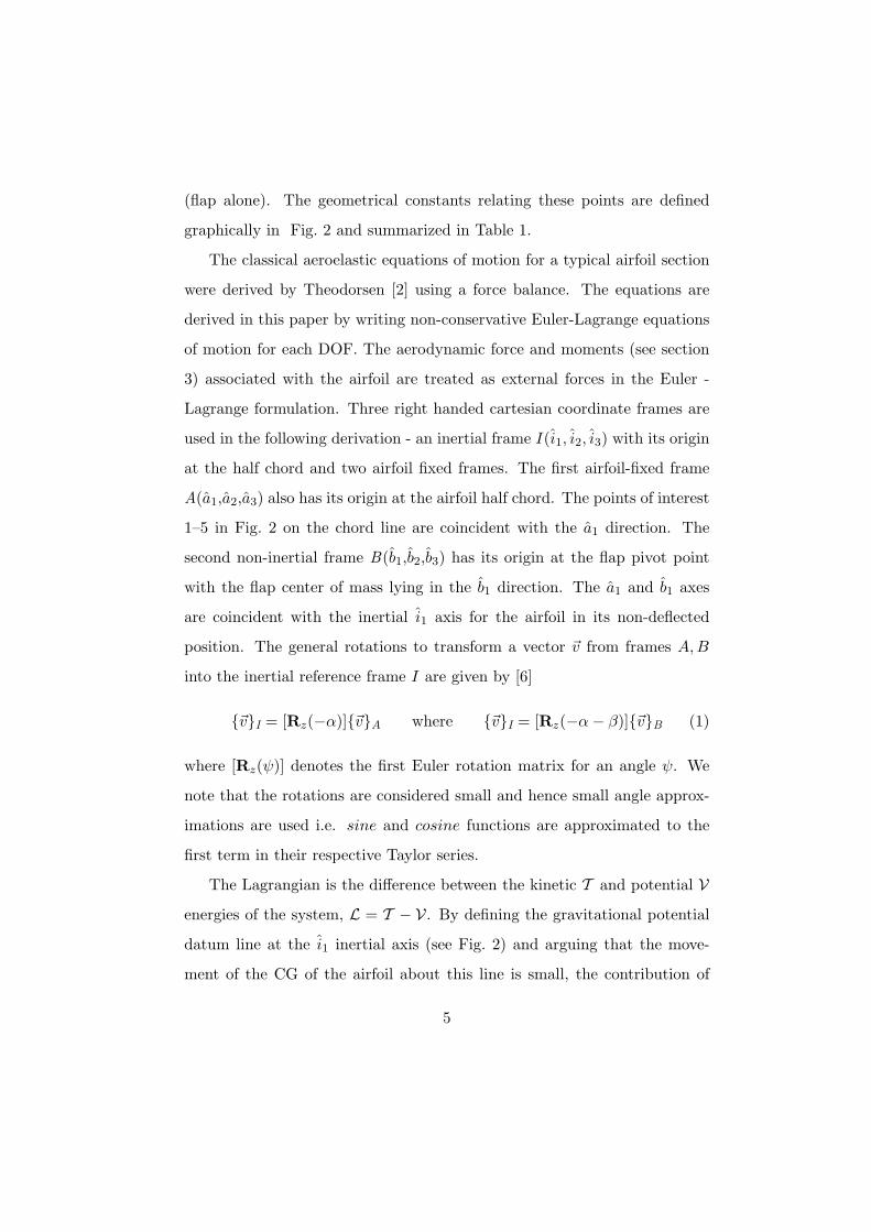
The classical aeroelastic equations of motion for a typical airfoil section

were derived by Theodorsen [2] using a force balance. The equations are

derived in this paper by writing non-conservative Euler-Lagrange equations

of motion for each DOF. The aerodynamic force and moments (see section

3) associated with the airfoil are treated as external forces in the Euler -

Lagrange formulation. Three right handed cartesian coordinate frames are

used in the following derivation - an inertial frame I (i1, i2, i3) with its origin

at the half chord and two airfoil fixed frames. The first airfoil-fixed frame

A(a1,a2,a3) also has its origin at the airfoil half chord. The points of interest

1–5 in Fig. 2 on the chord line are coincident with the a1 direction. The

second non-inertial frame B(b1,b2,b3) has its origin at the flap pivot point

with the flap center of mass lying in the b1 direction. The a1 and b1 axes

are coincident with the inertial i1 axis for the airfoil in its non-deflected

position. The general rotations to transform a vector ~v from frames A, B

into the inertial reference frame I are given by [6]

~vI = [Rz(−α)]~vA where ~vI = [Rz(−α − β)]~vB (1)

where [Rz(ψ)] denotes the first Euler rotation matrix for an angle ψ. We

note that the rotations are considered small and hence small angle approx-

imations are used i.e. sine and cosine functions are approximated to the

first term in their respective Taylor series.

The Lagrangian is the difference between the kinetic T and potential Venergies of the system, L = T − V. By defining the gravitational potential

datum line at the i1 inertial axis (see Fig. 2) and arguing that the move-

ment of the CG of the airfoil about this line is small, the contribution of

5

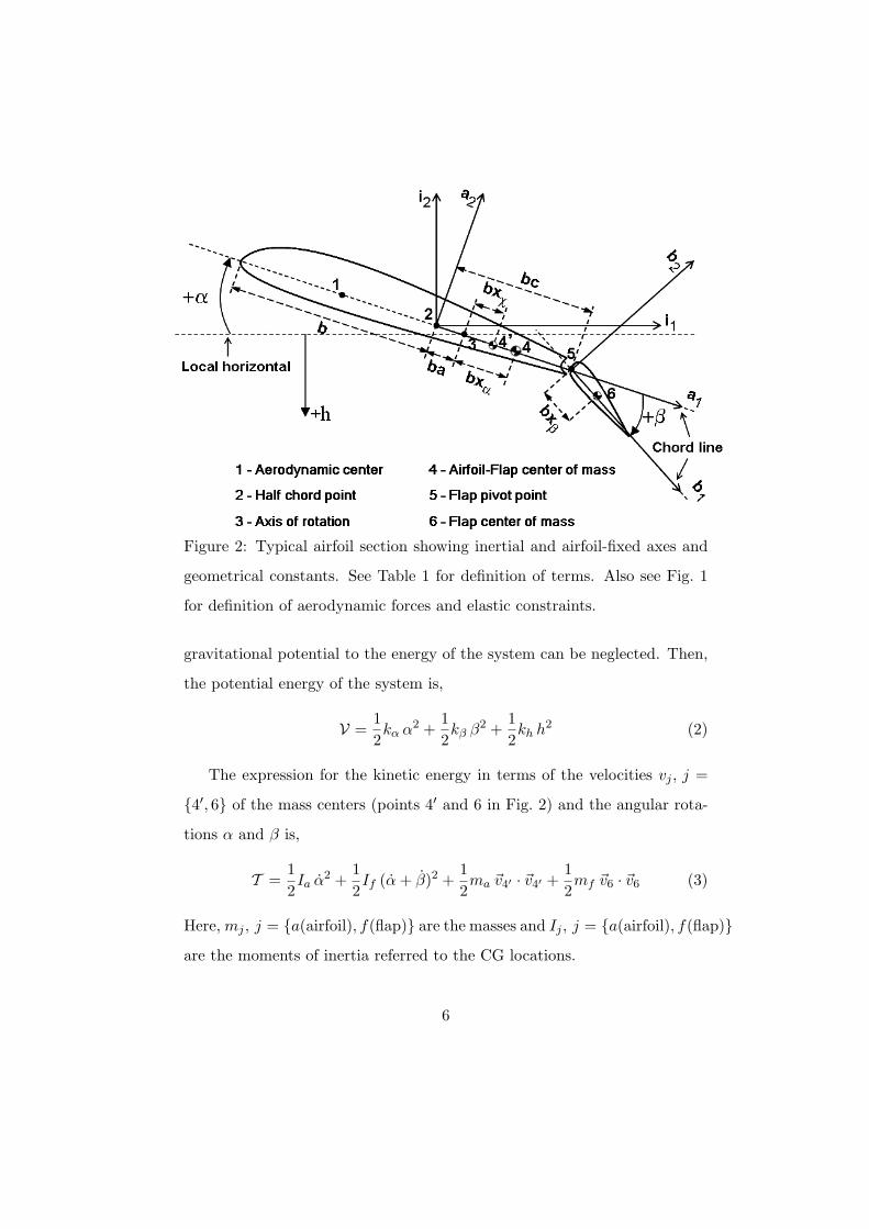
Figure 2: Typical airfoil section showing inertial and airfoil-fixed axes and

geometrical constants. See Table 1 for definition of terms. Also see Fig. 1

for definition of aerodynamic forces and elastic constraints.

gravitational potential to the energy of the system can be neglected. Then,

the potential energy of the system is,

V =1

2kα α2 +

1

2kβ β2 +

1

2kh h2 (2)

The expression for the kinetic energy in terms of the velocities vj , j =

4′, 6 of the mass centers (points 4′ and 6 in Fig. 2) and the angular rota-

tions α and β is,

T =1

2Ia α2 +

1

2If (α + β)2 +

1

2ma ~v4′ · ~v4′ +

1

2mf ~v6 · ~v6 (3)

Here, mj , j = a(airfoil), f(flap) are the masses and Ij , j = a(airfoil), f(flap)are the moments of inertia referred to the CG locations.

6

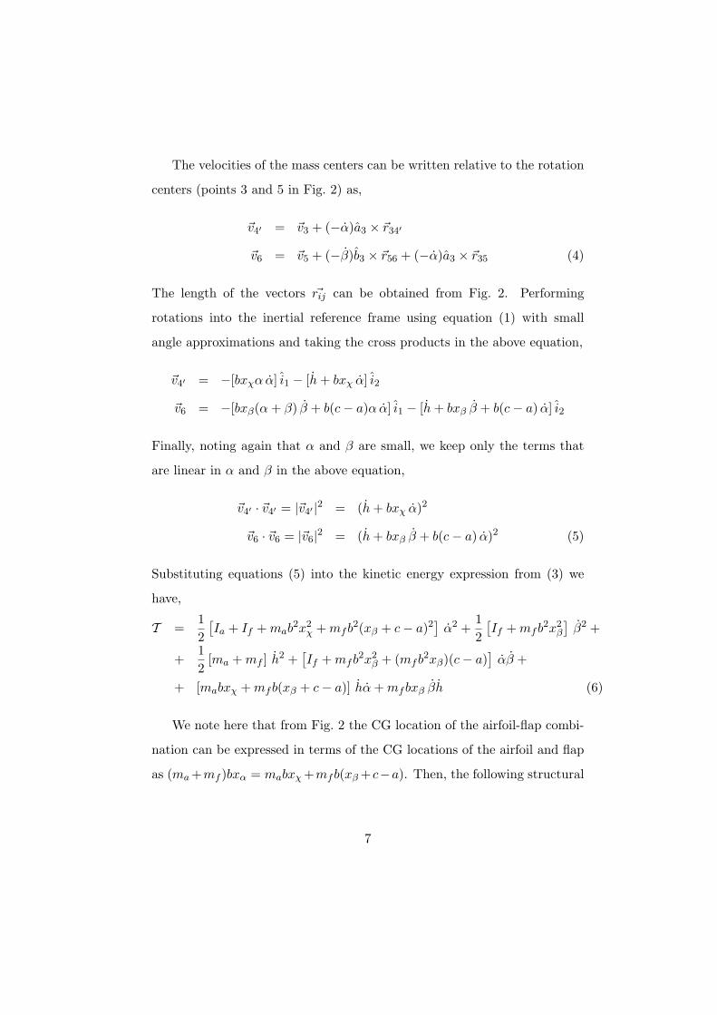
The velocities of the mass centers can be written relative to the rotation

centers (points 3 and 5 in Fig. 2) as,

~v4′ = ~v3 + (−α)a3 × ~r34′

~v6 = ~v5 + (−β)b3 × ~r56 + (−α)a3 × ~r35 (4)

The length of the vectors ~rij can be obtained from Fig. 2. Performing

rotations into the inertial reference frame using equation (1) with small

angle approximations and taking the cross products in the above equation,

~v4′ = −[bxχα α] i1 − [h + bxχ α] i2

~v6 = −[bxβ(α + β) β + b(c − a)α α] i1 − [h + bxβ β + b(c − a) α] i2

Finally, noting again that α and β are small, we keep only the terms that

are linear in α and β in the above equation,

~v4′ · ~v4′ = |~v4′ |2 = (h + bxχ α)2

~v6 · ~v6 = |~v6|2 = (h + bxβ β + b(c − a) α)2 (5)

Substituting equations (5) into the kinetic energy expression from (3) we

have,

T =1

2

[

Ia + If + mab2x2

χ + mfb2(xβ + c − a)2]

α2 +1

2

[

If + mfb2x2β

]

β2 +

+1

2[ma + mf ] h2 +

[

If + mfb2x2β + (mfb2xβ)(c − a)

]

αβ +

+ [mabxχ + mfb(xβ + c − a)] hα + mfbxβ βh (6)

We note here that from Fig. 2 the CG location of the airfoil-flap combi-

nation can be expressed in terms of the CG locations of the airfoil and flap

as (ma +mf )bxα = mabxχ +mfb(xβ +c−a). Then, the following structural

7

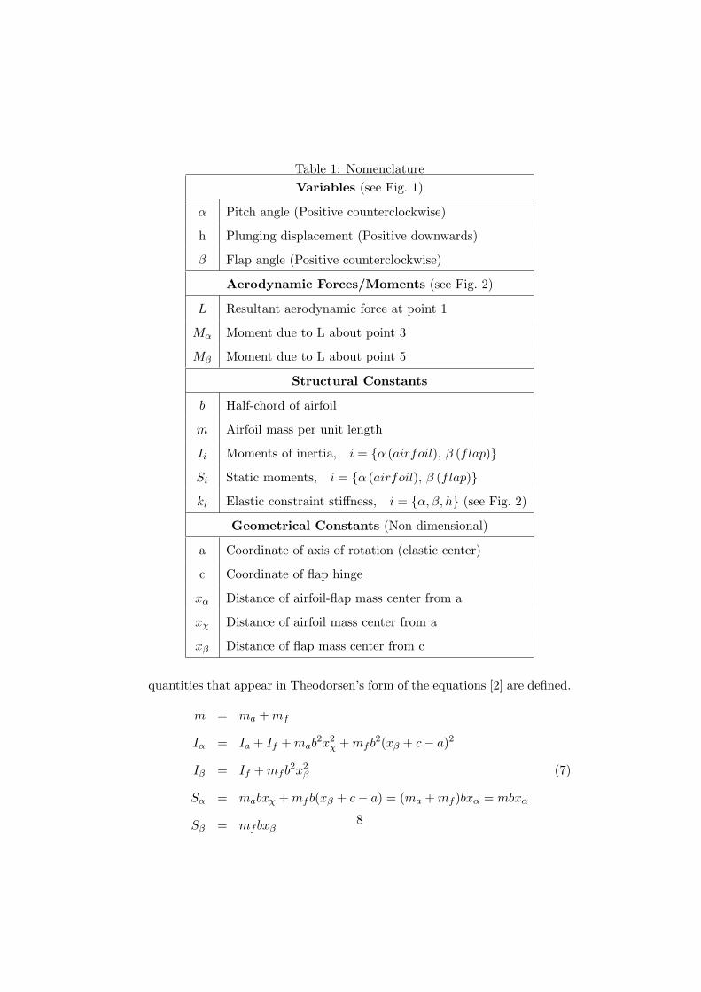
Table 1: Nomenclature

Variables (see Fig. 1)

α Pitch angle (Positive counterclockwise)

h Plunging displacement (Positive downwards)

β Flap angle (Positive counterclockwise)

Aerodynamic Forces/Moments (see Fig. 2)

L Resultant aerodynamic force at point 1

Mα Moment due to L about point 3

Mβ Moment due to L about point 5

Structural Constants

b Half-chord of airfoil

m Airfoil mass per unit length

Ii Moments of inertia, i = α (airfoil), β (flap)Si Static moments, i = α (airfoil), β (flap)ki Elastic constraint stiffness, i = α, β, h (see Fig. 2)

Geometrical Constants (Non-dimensional)

a Coordinate of axis of rotation (elastic center)

c Coordinate of flap hinge

xα Distance of airfoil-flap mass center from a

xχ Distance of airfoil mass center from a

xβ Distance of flap mass center from c

quantities that appear in Theodorsen’s form of the equations [2] are defined.

m = ma + mf

Iα = Ia + If + mab2x2

χ + mfb2(xβ + c − a)2

Iβ = If + mfb2x2β (7)

Sα = mabxχ + mfb(xβ + c − a) = (ma + mf )bxα = mbxα

Sβ = mfbxβ8

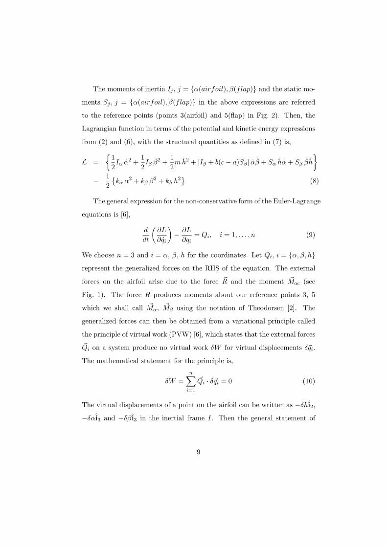
The moments of inertia Ij , j = α(airfoil), β(flap) and the static mo-

ments Sj , j = α(airfoil), β(flap) in the above expressions are referred

to the reference points (points 3(airfoil) and 5(flap) in Fig. 2). Then, the

Lagrangian function in terms of the potential and kinetic energy expressions

from (2) and (6), with the structural quantities as defined in (7) is,

L =

1

2Iα α2 +

1

2Iβ β2 +

1

2mh2 + [Iβ + b(c − a)Sβ ] αβ + Sα hα + Sβ βh

− 1

2

kα α2 + kβ β2 + kh h2

(8)

The general expression for the non-conservative form of the Euler-Lagrange

equations is [6],

d

dt

(

∂L

∂qi

)

− ∂L

∂qi= Qi, i = 1, . . . , n (9)

We choose n = 3 and i = α, β, h for the coordinates. Let Qi, i = α, β, hrepresent the generalized forces on the RHS of the equation. The external

forces on the airfoil arise due to the force ~R and the moment ~Mac (see

Fig. 1). The force R produces moments about our reference points 3, 5

which we shall call ~Mα, ~Mβ using the notation of Theodorsen [2]. The

generalized forces can then be obtained from a variational principle called

the principle of virtual work (PVW) [6], which states that the external forces

~Qi on a system produce no virtual work δW for virtual displacements δ~qi.

The mathematical statement for the principle is,

δW =n

∑

i=1

~Qi · δ~qi = 0 (10)

The virtual displacements of a point on the airfoil can be written as −δhi2,

−δαi3 and −δβ i3 in the inertial frame I. Then the general statement of

9

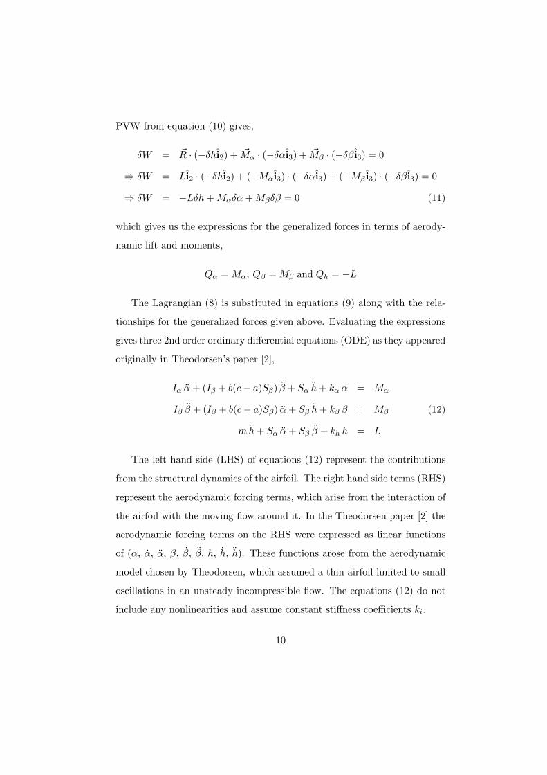
PVW from equation (10) gives,

δW = ~R · (−δhi2) + ~Mα · (−δαi3) + ~Mβ · (−δβ i3) = 0

⇒ δW = Li2 · (−δhi2) + (−Mαi3) · (−δαi3) + (−Mβ i3) · (−δβ i3) = 0

⇒ δW = −Lδh + Mαδα + Mβδβ = 0 (11)

which gives us the expressions for the generalized forces in terms of aerody-

namic lift and moments,

Qα = Mα, Qβ = Mβ and Qh = −L

The Lagrangian (8) is substituted in equations (9) along with the rela-

tionships for the generalized forces given above. Evaluating the expressions

gives three 2nd order ordinary differential equations (ODE) as they appeared

originally in Theodorsen’s paper [2],

Iα α + (Iβ + b(c − a)Sβ) β + Sα h + kα α = Mα

Iβ β + (Iβ + b(c − a)Sβ) α + Sβ h + kβ β = Mβ (12)

mh + Sα α + Sβ β + kh h = L

The left hand side (LHS) of equations (12) represent the contributions

from the structural dynamics of the airfoil. The right hand side terms (RHS)

represent the aerodynamic forcing terms, which arise from the interaction of

the airfoil with the moving flow around it. In the Theodorsen paper [2] the

aerodynamic forcing terms on the RHS were expressed as linear functions

of (α, α, α, β, β, β, h, h, h). These functions arose from the aerodynamic

model chosen by Theodorsen, which assumed a thin airfoil limited to small

oscillations in an unsteady incompressible flow. The equations (12) do not

include any nonlinearities and assume constant stiffness coefficients ki.

10

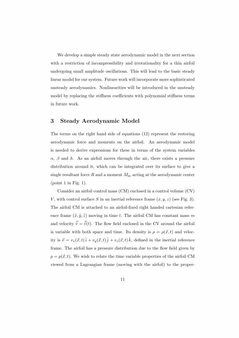
We develop a simple steady state aerodynamic model in the next section

with a restriction of incompressibility and irrotationality for a thin airfoil

undergoing small amplitude oscillations. This will lead to the basic steady

linear model for our system. Future work will incorporate more sophisticated

unsteady aerodynamics. Nonlinearities will be introduced in the unsteady

model by replacing the stiffness coefficients with polynomial stiffness terms

in future work.

3 Steady Aerodynamic Model

The terms on the right hand side of equations (12) represent the restoring

aerodynamic force and moments on the airfoil. An aerodynamic model

is needed to derive expressions for these in terms of the system variables

α, β and h. As an airfoil moves through the air, there exists a pressure

distribution around it, which can be integrated over its surface to give a

single resultant force R and a moment Mac acting at the aerodynamic center

(point 1 in Fig. 1).

Consider an airfoil control mass (CM) enclosed in a control volume (CV)

V , with control surface S in an inertial reference frame (x, y, z) (see Fig. 3).

The airfoil CM is attached to an airfoil-fixed right handed cartesian refer-

ence frame (x, y, z) moving in time t. The airfoil CM has constant mass m

and velocity ~v = ~v(t). The flow field enclosed in the CV around the airfoil

is variable with both space and time. Its density is ρ = ρ(~x, t) and veloc-

ity is ~v = vx(~x, t) i + vy(~x, t) j + vz(~x, t) k, defined in the inertial reference

frame. The airfoil has a pressure distribution due to the flow field given by

p = p(~x, t). We wish to relate the time variable properties of the airfoil CM

viewed from a Lagrangian frame (moving with the airfoil) to the proper-

11

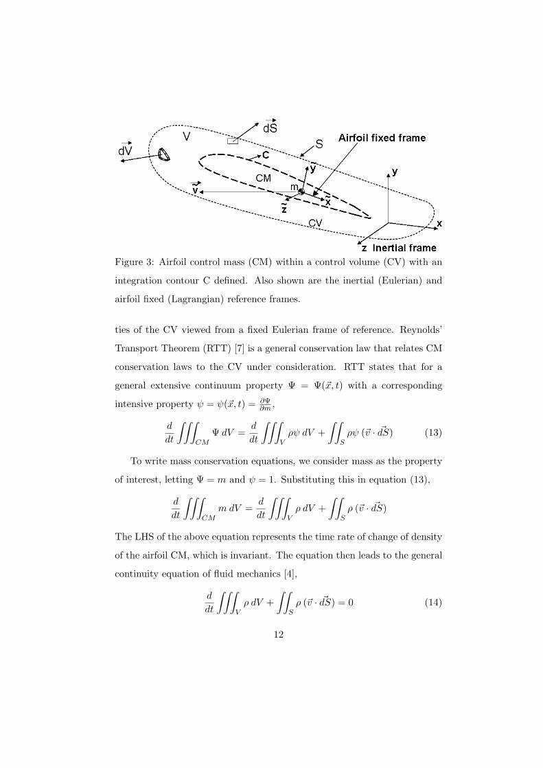
Figure 3: Airfoil control mass (CM) within a control volume (CV) with an

integration contour C defined. Also shown are the inertial (Eulerian) and

airfoil fixed (Lagrangian) reference frames.

ties of the CV viewed from a fixed Eulerian frame of reference. Reynolds’

Transport Theorem (RTT) [7] is a general conservation law that relates CM

conservation laws to the CV under consideration. RTT states that for a

general extensive continuum property Ψ = Ψ(~x, t) with a corresponding

intensive property ψ = ψ(~x, t) = ∂Ψ∂m

,

d

dt

∫∫∫

CM

Ψ dV =d

dt

∫∫∫

V

ρψ dV +

∫∫

S

ρψ (~v · ~dS) (13)

To write mass conservation equations, we consider mass as the property

of interest, letting Ψ = m and ψ = 1. Substituting this in equation (13),

d

dt

∫∫∫

CM

m dV =d

dt

∫∫∫

V

ρ dV +

∫∫

S

ρ (~v · ~dS)

The LHS of the above equation represents the time rate of change of density

of the airfoil CM, which is invariant. The equation then leads to the general

continuity equation of fluid mechanics [4],

d

dt

∫∫∫

V

ρ dV +

∫∫

S

ρ (~v · ~dS) = 0 (14)

12

For momentum conservation laws the continuum property of interest is

momentum. We let Ψ = m~v and correspondingly ψ = ~v. Then, substituting

this in the RTT equation (13),

d

dt

∫∫∫

CM

m~v dV =d

dt

∫∫∫

V

ρ~v dV +

∫∫

S

ρ~v (~v · ~dS) (15)

The LHS of equation (15) Newton’s 2nd Law (constant mass) relates the

momentum of the airfoil CM to the force it experiences,

~F = md

dt(~v) (16)

The force ~F on the airfoil CM is split into a volume force ~f acting on a

unit elemental volume dV , a force due to viscous shear stresses, represented

simply by ~Fviscous and a pressure force p acting on an elemental area dS.

Then, for the control volume V and control surface S, equation (15) gives,

−∫∫

S

p ~dS +

∫∫∫

V

ρ~f dV + ~Fviscous =∂

∂t

∫∫∫

V

ρ~v dV +

∫∫

S

(ρ~v · ~dS)~v (17)

The continuity and momentum conservation equations do not have closed

form solutions. To find closed form solutions to the equations, we impose

certain conditions on the flow properties. First, the flow around the airfoil is

assumed to be changing so slowly that a steady state in time can be assumed.

Second, the flow is assumed to be incompressible (a good approximation [4]

for a flow Mach number M < 0.3) making ρ = ρ∞ a constant, where the

subscript ∞ refers to freestream flow, far from the airfoil. Then, with these

assumptions and applying the divergence theorem to the continuity equation

(14),

ρ∞

∫∫

S

(~v · ~dS) = ρ∞

∫∫∫

V

(~∇ · ~v) dV = 0

⇒ ~∇ · ~v = 0 (18)

13

The third assumption is of irrotational flow which implies that the curl

of the velocity field ~∇ × ~v = 0. This allows us to define a potential flow

such that the velocity of the flow at every point is the gradient of a scalar

potential function φ(x, y, z):

~∇× ~v = 0 ⇔ ~v = ~∇φ(x, y, z). (19)

Immediately, from equations (18, 19) we obtain Laplace’s equation [4],

governing incompressible, irrotational flow.

∇2φ = 0 (20)

Since the equation is linear, a complicated flow about an airfoil can be

broken into several elementary potential flows that are solutions to Laplace’s

equation. This is the basis for Thin Airfoil Theory [8, 9] which we shall use

later. There are two boundary conditions [4] associated with equation (20)

for the case of flow over a solid body. The first assumes that perturbations go

to zero far from the body. Thus, we can define the freestream flow conditions

as being uniform [4] i.e. ~v = v∞i. The second is the flow tangency condition

for a solid body, which states that its physically impossible for a flow to cross

the solid body boundary i.e. ~∇φ · n = 0.

Now we take a look at the momentum conservation equation (17). The

irrotationality and incompressibility criteria imply that the flow is inviscid

i.e. friction, thermal conduction and diffusion effects are not present (these

effects are negligible for high Reynolds numbers associated with aircraft

flight [4]). We have already neglected inertial forces in our derivation of

the Euler-Lagrange equations and thus, ~f = 0. For the 2-dimensional airfoil

case, with unit depth in the z direction and the integration contour C defined

14

as shown in Fig. 3, equation (17) then reduces to:

−∮

C

p ~dS = ρ∞v∞

∮

C

(~v · ~dS) (21)

The LHS represents the force R due to the pressure distribution on the

airfoil. An expression for this can be calculated from either of the two

integrals in equation (21). However, since we have assumed incompressible,

irrotational flow, we can take advantage of the Kutta-Juokowski Theorem [4]

that relates the force (R) experienced by a two dimensional body of arbitrary

cross sectional area immersed in an incompressible, irrotational flow to the

magnitude of the circulation Γ around the body. Mathematically the Kutta-

Juokowski Theorem states,

~R = ρ∞ ~v∞ × ~Γ, where ~Γ = −∮

C

(~v · ~dS) (22)

Before moving onto Thin Airfoil Theory [8, 9], a brief discussion of the

inviscid flow assumption is in order. The condition of non-viscous flow

follows directly from the condition of irrotationality as a consequence of

Kelvin’s Theorem [4]. Kelvin’s theorem proves that for an inviscid flow, with

conservative body forces (in our case, body forces are zero), the circulation

remains constant along a closed contour. This implies that there is no change

in the vorticity, ~∇× ~v, with time:

dΓ

dt= − d

dt

∮

C

(~v · ~dS) = − d

dt

∫∫

S

(~∇× ~v) · ~dS = 0 (23)

If the vorticity is zero to begin with (as is the case for irrotational flow),

in the absence of inviscid forces the flow will remain irrotational. The major

drawback of ignoring viscosity is that zero drag is predicted for the airfoil

(d’Alembert’s paradox [4]). The paradox is apparent from equation (22).

The lift force L is defined as always being normal to the free stream while

15

the drag force D is always parallel to the flow (See Fig. 1). Taking force

components normal and parallel to the freestream flow,

L = ρ∞ | ~v∞| |~Γ| sin(π

2) = ρ∞v∞Γ

D = ρ∞ | ~v∞| |~Γ| sin(0) = 0 (24)

This paradox is resolved with the justification that the drag force is

always parallel to the translational DOF for the airfoil h and can thus be

safely ignored in our equations of motion. The line of action of the drag

force rotates about the mean chord line, but since we are assuming small

oscillations, any moments that could affect the two rotational DOF α and

β are neglected.

Classical Thin Airfoil Theory [8, 9] assumes that the flow around an

airfoil can be described by the superposition of two potential flows, such

that the entire flow around the airfoil has a velocity potential function that

is a solution to Laplace’s equation (20). The first potential flow is a uniform

freestream flow that we have already described, ~v = v∞i. To this is added

a second component of velocity, induced by the presence of the airfoil in the

moving flow.

The fundamental assumption of the theory is that the velocity induced by

the airfoil is equivalent to the sum of induced velocities of a line of elemental

vortices, called a vortex sheet, placed on the chord line of the airfoil (see

Fig. 4). Thus, the airfoil itself can be replaced by the vortex sheet in the

model. In reality, there is a thin layer of high vorticity on the surface of

the airfoil due to viscous effects and thus this model is somewhat justified,

with the restriction that the airfoil be thin enough to model with just the

chord line. The NACA [5] standard definition for a thin airfoil is that the

thickness be no greater than 10% of the chord i.e. tmax ≤ 0.1(2b), where

16

tmax is the maximum airfoil thickness and b is the half chord.

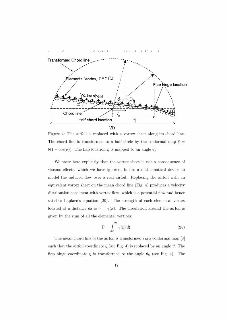
Figure 4: The airfoil is replaced with a vortex sheet along its chord line.

The chord line is transformed to a half circle by the conformal map ξ =

b(1 − cos(ϑ)). The flap location η is mapped to an angle θh.

We state here explicitly that the vortex sheet is not a consequence of

viscous effects, which we have ignored, but is a mathematical device to

model the induced flow over a real airfoil. Replacing the airfoil with an

equivalent vortex sheet on the mean chord line (Fig. 4) produces a velocity

distribution consistent with vortex flow, which is a potential flow and hence

satisfies Laplace’s equation (20). The strength of each elemental vortex

located at a distance dx is γ = γ(x). The circulation around the airfoil is

given by the sum of all the elemental vortices:

Γ =

∫ 2b

0γ(ξ) dξ (25)

The mean chord line of the airfoil is transformed via a conformal map [8]

such that the airfoil coordinate ξ (see Fig. 4) is replaced by an angle ϑ. The

flap hinge coordinate η is transformed to the angle θh (see Fig. 4). The

17

conformal map is given by the equation:

ξ = b(1 − cos(ϑ)) (26)

where, the flap hinge location in Fig. 4 is given by η = b(1 − cos(θh)).

The lift per unit span, L = ρ∞v∞Γ follows from the Kutta-Joukowski

Theorem (22). At this point, it is convenient to introduce a dimensionless

variable known as the section lift coefficient [4], defined as,

cl =L

12ρ∞v2

∞(2b)

=L

bρ∞v2∞

=Γ

bv∞(27)

where b is the half chord length from Fig. 2. From the Buckhingam Pi

theorem [4], in general for a given flow cl = cl(α, β). Expanding this with a

first order Taylor approximation,

cl = cl(0, 0) +∂cl

∂αα +

∂cl

∂ββ (28)

Thin airfoil theory [8] gives constant expressions for the partial derivatives in

equation (28). We are assuming a symmetric airfoil, which makes cl(0, 0) =

0 [4]. Then,

cl = [2π] α + 2[(π − θh) + sin(θh)] β

Noting that the length of the flap chord from Fig. 2 and Fig. 4 b(1−c) = b−η

and using the inverse of the conformal map defined in equation (26),

cl = σ1 α + σ2 β (29)

where σ1, σ2 are constant value expressions in terms of the geometrical length

c (see Fig. 2).

The aerodynamic moment about an arbitrary point x0 on the airfoil can

be expressed in terms of the strength γ of each elemental vortex as,

M = −ρ∞v∞

∫ 2b

0(ξ − x0) γ(ξ − x0) dξ

18

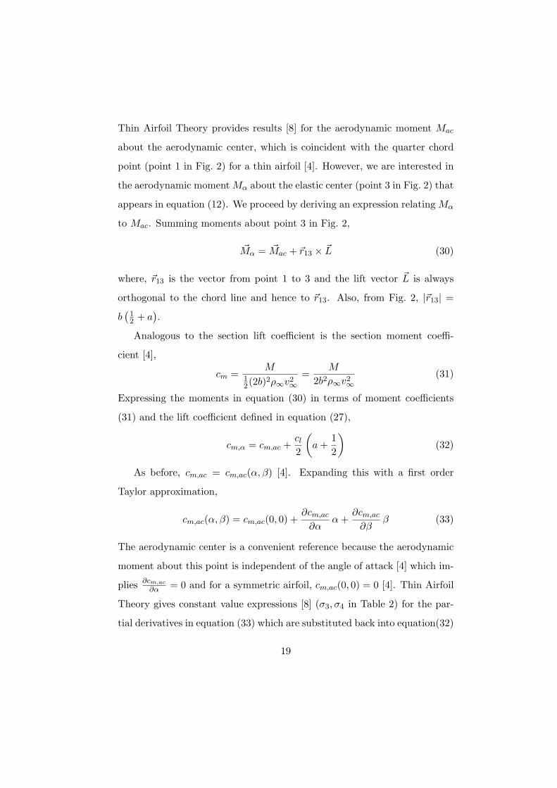
Thin Airfoil Theory provides results [8] for the aerodynamic moment Mac

about the aerodynamic center, which is coincident with the quarter chord

point (point 1 in Fig. 2) for a thin airfoil [4]. However, we are interested in

the aerodynamic moment Mα about the elastic center (point 3 in Fig. 2) that

appears in equation (12). We proceed by deriving an expression relating Mα

to Mac. Summing moments about point 3 in Fig. 2,

~Mα = ~Mac + ~r13 × ~L (30)

where, ~r13 is the vector from point 1 to 3 and the lift vector ~L is always

orthogonal to the chord line and hence to ~r13. Also, from Fig. 2, |~r13| =

b(

12 + a

)

.

Analogous to the section lift coefficient is the section moment coeffi-

cient [4],

cm =M

12(2b)2ρ∞v2

∞

=M

2b2ρ∞v2∞

(31)

Expressing the moments in equation (30) in terms of moment coefficients

(31) and the lift coefficient defined in equation (27),

cm,α = cm,ac +cl

2

(

a +1

2

)

(32)

As before, cm,ac = cm,ac(α, β) [4]. Expanding this with a first order

Taylor approximation,

cm,ac(α, β) = cm,ac(0, 0) +∂cm,ac

∂αα +

∂cm,ac

∂ββ (33)

The aerodynamic center is a convenient reference because the aerodynamic

moment about this point is independent of the angle of attack [4] which im-

plies∂cm,ac

∂α= 0 and for a symmetric airfoil, cm,ac(0, 0) = 0 [4]. Thin Airfoil

Theory gives constant value expressions [8] (σ3, σ4 in Table 2) for the par-

tial derivatives in equation (33) which are substituted back into equation(32)

19

Table 2: Thin Airfoil Theory expressions for aerodynamic coefficients

Partial Symbol Constant value expression

derivative

∂cl

∂ασ1 2 π

∂cl

∂βσ2 2 [arccos(c) +

√1 − c2]

∂cm,ac

∂ασ3 0

∂cm,ac

∂βσ4 −1

2(1 + c)√

1 − c2

∂cm,α

∂ασ5 π

(

12 + a

)

∂cm,α

∂βσ6

(

12 + a

)

arccos(c) +(

a − c2

) √1 − c2

∂cm,β

∂ασ7

2(1−c)2

2(1 + 2c)(

π2 − arccos

√

1−c2

)

− (c + 2)√

1 − c2

∂cm,β

∂βσ8 σ7

1 − 1π

(

2 arccos√

1−c2 −

√1 − c2

)

+[

4σ4

π(1−c)2

] [

π − 2 arccos√

1−c2 −

√1 − c2

]

along with the expression for cl from equation (29) to obtain,

cm,α = σ5 α + σ6 β (34)

where the constant terms σ5, σ6 are given in Table 2.

The hinge moment Mβ about the flap hinge (point 5 in Fig. 2) arises

due to the pressure distribution on the flap. The hinge moment about an

arbitrary point x0 on the flap can be expressed in terms of the strength γ

of the elemental vortices arranged along the flap chord as,

Mβ = −ρ∞v∞

∫ b

bc

(ξ − x0) γ(ξ − x0) dη

As before, a section hinge moment coefficient is defined with the airfoil chord

b replaced by the flap chord b(1 − c) (see Fig. 2),

cm,β = cm,β(α, β) =Mβ

12(b(1 − c))2ρ∞v2

∞

(35)

20

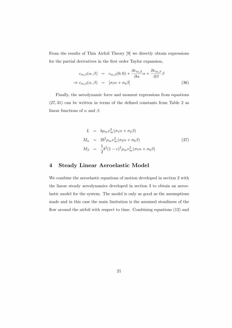
From the results of Thin Airfoil Theory [9] we directly obtain expressions

for the partial derivatives in the first order Taylor expansion,

cm,β(α, β) = cm,β(0, 0) +∂cm,β

∂αα +

∂cm,β

∂ββ

⇒ cm,β(α, β) = [σ7α + σ8β] (36)

Finally, the aerodynamic force and moment expressions from equations

(27, 31) can be written in terms of the defined constants from Table 2 as

linear functions of α and β.

L = bρ∞v2∞

(σ1α + σ2β)

Mα = 2b2ρ∞v2∞

(σ5α + σ6β) (37)

Mβ =1

2b2(1 − c)2ρ∞v2

∞(σ7α + σ8β)

4 Steady Linear Aeroelastic Model

We combine the aeroelastic equations of motion developed in section 2 with

the linear steady aerodynamics developed in section 3 to obtain an aeroe-

lastic model for the system. The model is only as good as the assumptions

made and in this case the main limitation is the assumed steadiness of the

flow around the airfoil with respect to time. Combining equations (12) and

21

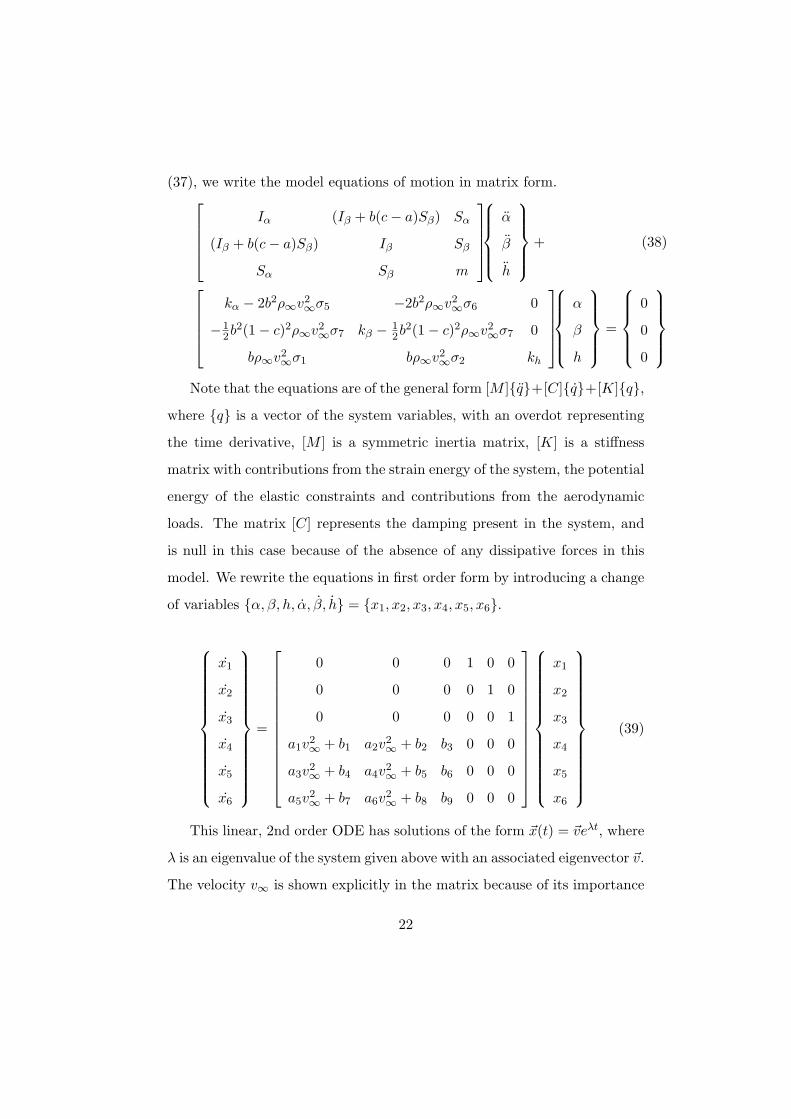
(37), we write the model equations of motion in matrix form.

Iα (Iβ + b(c − a)Sβ) Sα

(Iβ + b(c − a)Sβ) Iβ Sβ

Sα Sβ m

α

β

h

+ (38)

kα − 2b2ρ∞v2∞

σ5 −2b2ρ∞v2∞

σ6 0

−12b2(1 − c)2ρ∞v2

∞σ7 kβ − 1

2b2(1 − c)2ρ∞v2∞

σ7 0

bρ∞v2∞

σ1 bρ∞v2∞

σ2 kh

α

β

h

=

0

0

0

Note that the equations are of the general form [M ]q+[C]q+[K]q,where q is a vector of the system variables, with an overdot representing

the time derivative, [M ] is a symmetric inertia matrix, [K] is a stiffness

matrix with contributions from the strain energy of the system, the potential

energy of the elastic constraints and contributions from the aerodynamic

loads. The matrix [C] represents the damping present in the system, and

is null in this case because of the absence of any dissipative forces in this

model. We rewrite the equations in first order form by introducing a change

of variables α, β, h, α, β, h = x1, x2, x3, x4, x5, x6.

x1

x2

x3

x4

x5

x6

=

0 0 0 1 0 0

0 0 0 0 1 0

0 0 0 0 0 1

a1v2∞

+ b1 a2v2∞

+ b2 b3 0 0 0

a3v2∞

+ b4 a4v2∞

+ b5 b6 0 0 0

a5v2∞

+ b7 a6v2∞

+ b8 b9 0 0 0

x1

x2

x3

x4

x5

x6

(39)

This linear, 2nd order ODE has solutions of the form ~x(t) = ~veλt, where

λ is an eigenvalue of the system given above with an associated eigenvector ~v.

The velocity v∞ is shown explicitly in the matrix because of its importance

22

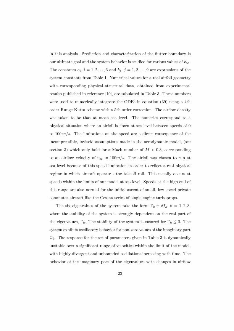
in this analysis. Prediction and characterization of the flutter boundary is

our ultimate goal and the system behavior is studied for various values of v∞.

The constants ai, i = 1, 2 . . . , 6 and bj , j = 1, 2 . . . , 9 are expressions of the

system constants from Table 1. Numerical values for a real airfoil geometry

with corresponding physical structural data, obtained from experimental

results published in reference [10], are tabulated in Table 3. These numbers

were used to numerically integrate the ODEs in equation (39) using a 4th

order Runge-Kutta scheme with a 5th order correction. The airflow density

was taken to be that at mean sea level. The numerics correspond to a

physical situation where an airfoil is flown at sea level between speeds of 0

to 100m/s. The limitations on the speed are a direct consequence of the

incompressible, inviscid assumptions made in the aerodynamic model, (see

section 3) which only hold for a Mach number of M < 0.3, corresponding

to an airflow velocity of v∞ ≈ 100m/s. The airfoil was chosen to run at

sea level because of this speed limitation in order to reflect a real physical

regime in which aircraft operate - the takeoff roll. This usually occurs at

speeds within the limits of our model at sea level. Speeds at the high end of

this range are also normal for the initial ascent of small, low speed private

commuter aircraft like the Cessna series of single engine turboprops.

The six eigenvalues of the system take the form Γk ± ıΩk, k = 1, 2, 3,

where the stability of the system is strongly dependent on the real part of

the eigenvalues, Γk. The stability of the system is ensured for Γk ≤ 0. The

system exhibits oscillatory behavior for non-zero values of the imaginary part

Ωk. The response for the set of parameters given in Table 3 is dynamically

unstable over a significant range of velocities within the limit of the model,

with highly divergent and unbounded oscillations increasing with time. The

behavior of the imaginary part of the eigenvalues with changes in airflow

23

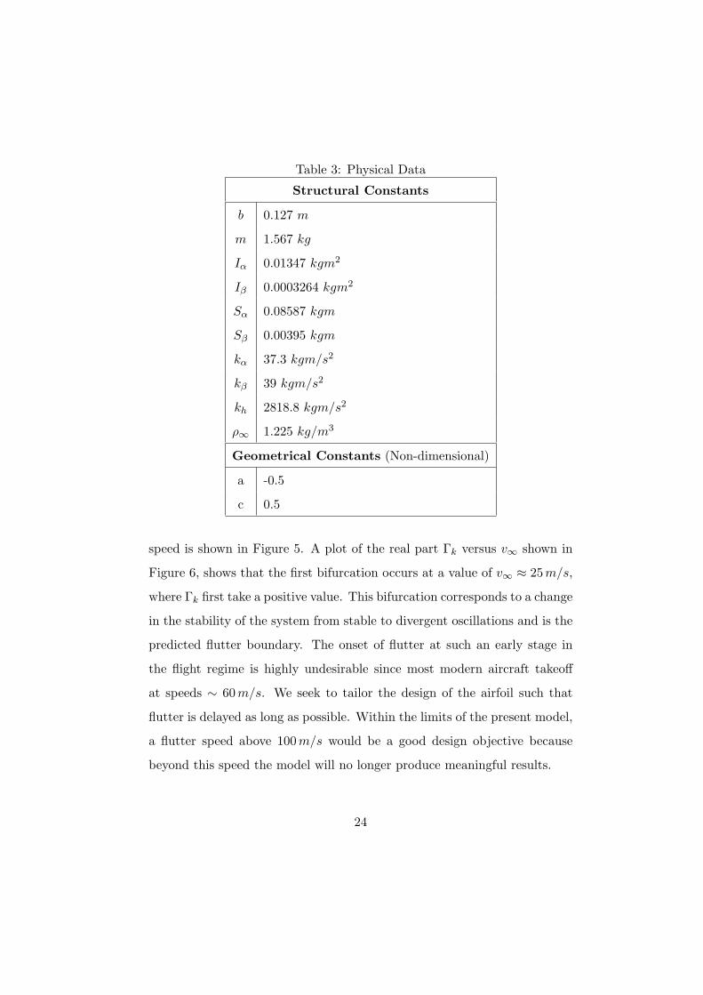
Table 3: Physical Data

Structural Constants

b 0.127 m

m 1.567 kg

Iα 0.01347 kgm2

Iβ 0.0003264 kgm2

Sα 0.08587 kgm

Sβ 0.00395 kgm

kα 37.3 kgm/s2

kβ 39 kgm/s2

kh 2818.8 kgm/s2

ρ∞ 1.225 kg/m3

Geometrical Constants (Non-dimensional)

a -0.5

c 0.5

speed is shown in Figure 5. A plot of the real part Γk versus v∞ shown in

Figure 6, shows that the first bifurcation occurs at a value of v∞ ≈ 25 m/s,

where Γk first take a positive value. This bifurcation corresponds to a change

in the stability of the system from stable to divergent oscillations and is the

predicted flutter boundary. The onset of flutter at such an early stage in

the flight regime is highly undesirable since most modern aircraft takeoff

at speeds ∼ 60 m/s. We seek to tailor the design of the airfoil such that

flutter is delayed as long as possible. Within the limits of the present model,

a flutter speed above 100m/s would be a good design objective because

beyond this speed the model will no longer produce meaningful results.

24

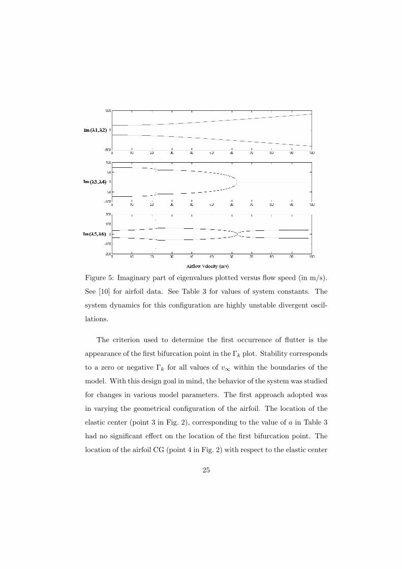
Figure 5: Imaginary part of eigenvalues plotted versus flow speed (in m/s).

See [10] for airfoil data. See Table 3 for values of system constants. The

system dynamics for this configuration are highly unstable divergent oscil-

lations.

The criterion used to determine the first occurrence of flutter is the

appearance of the first bifurcation point in the Γk plot. Stability corresponds

to a zero or negative Γk for all values of v∞ within the boundaries of the

model. With this design goal in mind, the behavior of the system was studied

for changes in various model parameters. The first approach adopted was

in varying the geometrical configuration of the airfoil. The location of the

elastic center (point 3 in Fig. 2), corresponding to the value of a in Table 3

had no significant effect on the location of the first bifurcation point. The

location of the airfoil CG (point 4 in Fig. 2) with respect to the elastic center

25

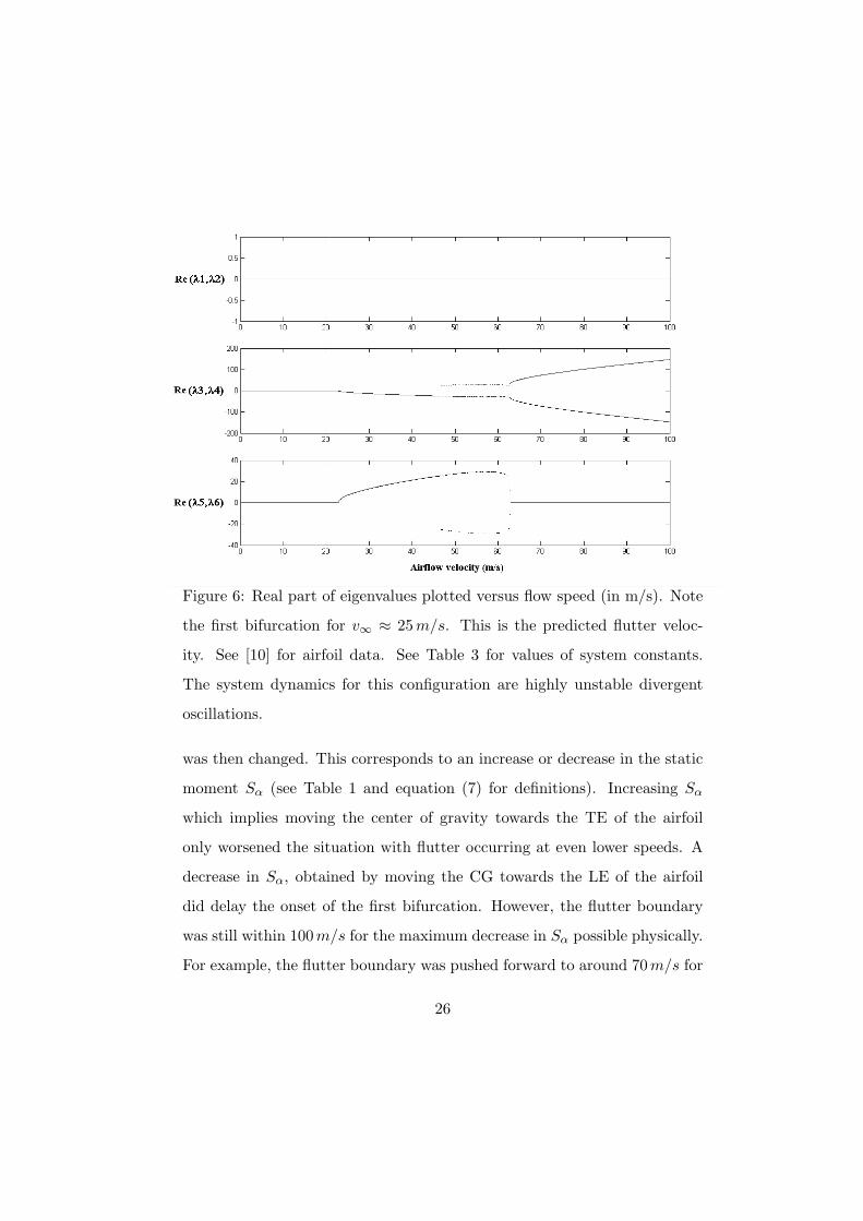
Figure 6: Real part of eigenvalues plotted versus flow speed (in m/s). Note

the first bifurcation for v∞ ≈ 25 m/s. This is the predicted flutter veloc-

ity. See [10] for airfoil data. See Table 3 for values of system constants.

The system dynamics for this configuration are highly unstable divergent

oscillations.

was then changed. This corresponds to an increase or decrease in the static

moment Sα (see Table 1 and equation (7) for definitions). Increasing Sα

which implies moving the center of gravity towards the TE of the airfoil

only worsened the situation with flutter occurring at even lower speeds. A

decrease in Sα, obtained by moving the CG towards the LE of the airfoil

did delay the onset of the first bifurcation. However, the flutter boundary

was still within 100m/s for the maximum decrease in Sα possible physically.

For example, the flutter boundary was pushed forward to around 70m/s for

26

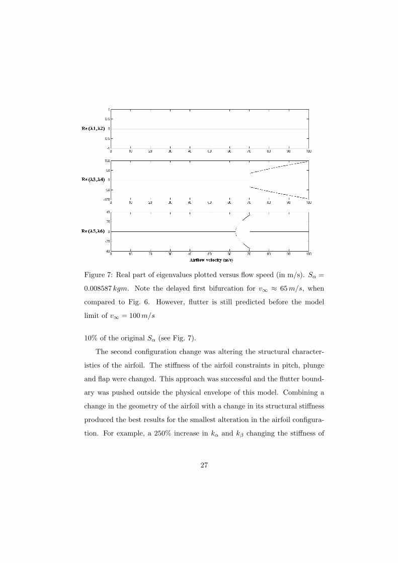
Figure 7: Real part of eigenvalues plotted versus flow speed (in m/s). Sα =

0.008587 kgm. Note the delayed first bifurcation for v∞ ≈ 65 m/s, when

compared to Fig. 6. However, flutter is still predicted before the model

limit of v∞ = 100m/s

10% of the original Sα (see Fig. 7).

The second configuration change was altering the structural character-

istics of the airfoil. The stiffness of the airfoil constraints in pitch, plunge

and flap were changed. This approach was successful and the flutter bound-

ary was pushed outside the physical envelope of this model. Combining a

change in the geometry of the airfoil with a change in its structural stiffness

produced the best results for the smallest alteration in the airfoil configura-

tion. For example, a 250% increase in kα and kβ changing the stiffness of

27

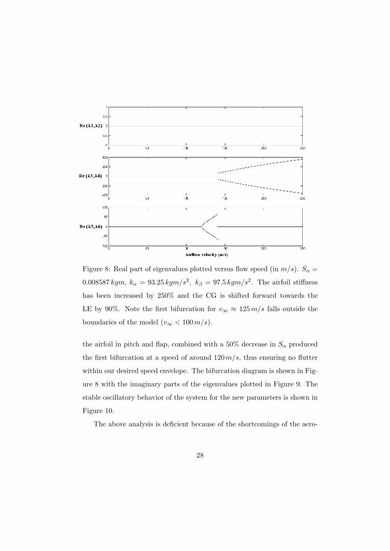
Figure 8: Real part of eigenvalues plotted versus flow speed (in m/s). Sα =

0.008587 kgm, kα = 93.25 kgm/s2, kβ = 97.5 kgm/s2. The airfoil stiffness

has been increased by 250% and the CG is shifted forward towards the

LE by 90%. Note the first bifurcation for v∞ ≈ 125 m/s falls outside the

boundaries of the model (v∞ < 100 m/s).

the airfoil in pitch and flap, combined with a 50% decrease in Sα produced

the first bifurcation at a speed of around 120m/s, thus ensuring no flutter

within our desired speed envelope. The bifurcation diagram is shown in Fig-

ure 8 with the imaginary parts of the eigenvalues plotted in Figure 9. The

stable oscillatory behavior of the system for the new parameters is shown in

Figure 10.

The above analysis is deficient because of the shortcomings of the aero-

28

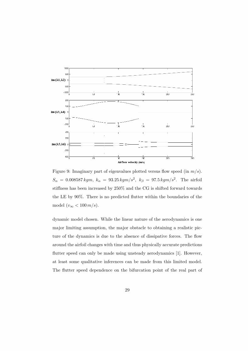
Figure 9: Imaginary part of eigenvalues plotted versus flow speed (in m/s).

Sα = 0.008587 kgm, kα = 93.25 kgm/s2, kβ = 97.5 kgm/s2. The airfoil

stiffness has been increased by 250% and the CG is shifted forward towards

the LE by 90%. There is no predicted flutter within the boundaries of the

model (v∞ < 100 m/s).

dynamic model chosen. While the linear nature of the aerodynamics is one

major limiting assumption, the major obstacle to obtaining a realistic pic-

ture of the dynamics is due to the absence of dissipative forces. The flow

around the airfoil changes with time and thus physically accurate predictions

flutter speed can only be made using unsteady aerodynamics [1]. However,

at least some qualitative inferences can be made from this limited model.

The flutter speed dependence on the bifurcation point of the real part of

29

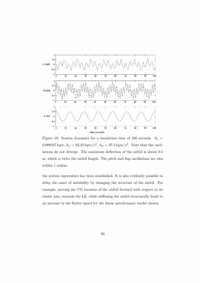
Figure 10: System dynamics for a simulation time of 100 seconds. Sα =

0.008587 kgm, kα = 93.25 kgm/s2, kβ = 97.5 kgm/s2. Note that the oscil-

lations do not diverge. The maximum deflection of the airfoil is about 0.5

m, which is twice the airfoil length. The pitch and flap oscillations are also

within 1 radian.

the system eigenvalues has been established. It is also evidently possible to

delay the onset of instability by changing the structure of the airfoil. For

example, moving the CG location of the airfoil forward with respect to its

elastic axis, towards the LE, while stiffening the airfoil structurally leads to

an increase in the flutter speed for the linear aerodynamic model chosen.

30

5 Concluding Remarks

In this paper, a linear steady state aeroelastic model in 3 DOF was derived

a priori for a 2 dimensional airfoil model. The equations of motion were

derived from the Lagrangian formulation for conservative systems. A flut-

ter boundary was predicted at sea level conditions and the effects of airfoil

geometry and structural characteristics on the predicted value were stud-

ied. The results indicate that a linear steady state model cannot accurately

predict the flutter boundary. The weakness in the model lies entirely in

the assumed steadiness of the airflow around an airfoil. There are several

perturbative effects introduced into the flow due to the movement of the air-

foil that are entirely neglected. Furthermore, the steady state assumption

limits the velocity range for which this model is valid, due to the necessary

preconditions of inviscidity and incompressibility that have been introduced

while deriving the aerodynamical model. However, the model does provide

a certain amount of insight into the nature of the flutter boundary. It is

shown that the flutter boundary can be inferred from the behavior of the

real part of the eigenvalues arising from the equations of motion. It has

also been noticed that changing certain airfoil structural and geometrical

parameters leads to a shift in the position of the flutter boundary. This

is significant because it allows for the design of an airfoil which will never

encounter flutter for a certain flight regime.

The development of unsteady aerodynamics to complement the struc-

tural equations derived earlier in this paper is the logical next step. The

introduction of dissipative forces into the flow around an airfoil will lead

to a more realistic prediction of flutter characteristics. A readily available

and widely used [1] unsteady aerodynamic theory is Peters’ finite state,

31

induced-flow theory. Subsequent work should include results from this the-

ory in the aerodynamics of the model derived in this paper. In Peters’

theory, the aerodynamic forcing functions can be expressed as functions of

time derivatives of the system variables, such that L = L(α, β, h, α, β, h),

Mα = Mα(α, β, h, α, β, h), Mα = Mα(α, β, h, α, β, h). The second step will

be incorporating structural nonlinearities into the unsteady model. This

will be effected by replacing the structural stiffness constants kα, kβ, kh with

polynomial stiffness coefficients kα(α), kβ(β), kh(h).

Acknowledgements

I would like to thank my undergraduate research advisor Dr. Mason Porter

of the School of Mathematics and Dr. Slaven Peles of the Center for Non-

linear Science in the School of Physics for their guidance and support. I am

grateful to Dr. Dewey Hodges and my undergraduate advisor Dr. Marilyn

Smith of the School of Aerospace Engineering for their invaluable advice.

References

[1] Dewey H. Hodges and G. Alvin Pierce. Introduction to Structural Dy-

namics and Aeroelasticity. Cambridge University Press, first edition,

2002.

[2] Theodore Theodorsen. General theory of aerodynamic instability and

the mechanism of flutter. NACA Technical Report 496, 1935.

[3] B.H.K. Lee, S.J. Price, and Y.S. Wong. Nonlinear aeroelastic analy-

sis of airfoils: bifurcation and chaos. Progress in Aerospace Sciences,

(35):205–334, 1999.

32

[4] John D. Anderson Jr. Fundamentals of Aerodynamics. McGraw-Hill,

third edition, 2001.

[5] Ira H. Abbott and Albert E. von Doenhoff. Theory of Wing Sections.

Dover Publications, first dover edition, 1959.

[6] Herbert Goldstein, Charles P. Poole Jr, and John L. Safko. Classical

Mechanics. Addison Wesley, third edition, 2003.

[7] Frank M. White. Fluid Mechanics. Mc Graw Hill, fifth edition, 2002.

[8] Arnold M. Kuethe and Chuen-Yen Chow. Foundations of Aerodynamics

- Bases of Aerodynamic Design. John Wiley and Sons, fifth edition,

1998.

[9] Hermann Glauert. Theoretical relationships for an aerofoil with hinged

flap. ARC Reports and Memoranda 1095, Aeronautical Research Com-

mittee, 1927.

[10] E.H. Dowell, J.P. Thomas, and K.C. Hall. Transonic limit cycle os-

cillation analysis using reduced order aerodynamic models. Journal of

Fluids and Structures, (19):17–27, 2004.

33