eee 481 computer controlled systems - …tsakalis.faculty.asu.edu/notes/e481.pdf · eee 481...
TRANSCRIPT

1
EEE 481 Computer Controlled Systems
• Course outline
• (rev 9/2/15)
Wk 1: Introduction, Matlab and Simulink, PC104 platform, System simulation and Real-Time applications (Notes) Wk 2: Computer Interfacing for Data Acquisition and Control, ADC-DAC, Signal conditioning, quantization (Notes) Wk 3: Review of Z-transform and State Variables (Ch.2) Wk 4: Z-transform and state variables, Linearization (Ch.2) Wk 5: Sampling and Reconstruction, CT-DT conversions, Discretization (Ch.3, Notes) Wk 6: Discretization, Open-loop DT systems (Ch.4, Notes) Wk 7: Closed-Loop systems, Time/Frequency response characteristics (Notes, Ch. 5,6) Wk 8-9: Feedback and Feedforward Control, Stability Analysis, Nyquist/Bode (Notes, Ch. 7) Wk 10: PID controllers and tuning (Notes, Ch.8: Specs, PID) Wk 11: PID tuning and Controller Discretization (Notes) Wk 12: Feedforward Compensation (Notes) Wk 13: State Estimation (Ch.9: Observers) Wk 14: Model Identification (Notes, Ch. 10) Wk 15: Sensors, Actuators (Notes)

2
Introduction: The PC-104 Standard
• Low-power, general-purpose embedded applications
• Standard (small) size, stackable – Sound, PCMCIA, GPS, additional LAN, ADC-DAC,+…
• Advantech’s PCM 3350 – Stable geode processor (Pentium 300Mhz), on-chip PCI
VGA, Intel82559 ER high performance Ethernet chip – 2 RS-232 serial ports – 128M RAM and FLASH memory (replacing the hard
drive)

3
Introduction: The PC-104 Standard
• MATLAB compatibility: supported Ethernet chip for fast code download and testing. – Not crucial; one serial port can satisfy
MATLAB’s requirement for a comm. link; but communication is very slow and the port is lost to the application.
– check details in the web (advantech.com)
• Operating system: DOS or Windows (CE). – DOS suffices for downloading MATLAB’s real-
time kernel and application program

4
Introduction: The PC-104 Standard
• Data acquisition and Control board: Diamond MM – Analog-to-Digital Conversion (ADC or A/D): 16 single ended or
8 differential analog inputs, 12-bit resolution, 2kHz software, 20kHz interrupt routine, 100kHz in DMA operation
– Digital-to-Analog Conversion (DAC or D/A): 2 analog outputs, 12-bit resolution
– 16 digital I/O lines (8 in, 8 out) – MATLAB compatibility: important to obtain quick results; but
it offers only partial access to the board functions – web page: diamondsystems.com

5
Introduction to Computers
• Microprocessor, motherboard, memory – address, data, control buses – CPU: Arithmetic Logic Unit, Accumulator,
Program Counter, Instruction Register, Condition Codes Register, Control Unit, Clock speed, MIPS, FLOPS
– TPA (Transient Program Area): operating system, Commands, I/O, BIOS, Interrupt vector
– XMS (Extended Memory System)

6
Introduction to Computers
• Memory characteristics (older data)
TYPE AVG.CAPAC.
AVG.ACCESS
REL.COST
Cache 0.5M 2ns 10
Main 50M 20ns 1
Hard Disk 50G 10ms 10-2
Floppy Disk 10M 500ms 10-3
MagneticTape
5G 25s 10-3
CDROM 600M 500ms 10-4
DVDROM 8G 500ms 10-5

7
Introduction to Computers
• I/O interfaces – isolated (IN-OUT instructions) and memory-
mapped I/O
• Communication with external devices – polling: checking each device for service
periodically (simple but inefficient) – interrupts: each device generates an interrupt
that is serviced according to its priority level, in case of simultaneous arrivals

8
Introduction to Computers
• Arithmetic Computations (7 x 6, 7/2) – Integer:
• 0111 x 0110 = 01110+011100 = 101010 • 0111 / 0010 = (011.1) = 011 • Answer length increases by one bit in additions and one word in
multiplications. Scaling and truncation is necessary for fixed word lengths
– Floating point: (binary 5e3 format) • 0.11100e011 x 0.11000e011 =
(0.01110+0.00111)e011+011 = 0.10101e110 • 0.111e011 / 0.100e010 = (1.11)e011-010 =
0.111e010

9
Introduction to Computers
• Math coprocessors perform a large variety of arithmetic operations (+,-,x,/,sqrt,sin,log,…) – fast and high precision – hardware implementation of operations – computation uses algorithms and look-up tables – Newer CPUs have a built-in math coprocessor;
nowadays, they are only absent in very-low-cost, or very-fast applications

10
Introduction: Parallel Communication
• Timing circuits: counters and clocks – Real-time applications require independent
clocks that are not affected by processor operations
• Parallel I/O port, parallel interface adapter (PIA)
CPU PIA External Interface Hardware
address bus
data bus
control lines
Peripheral devices
11
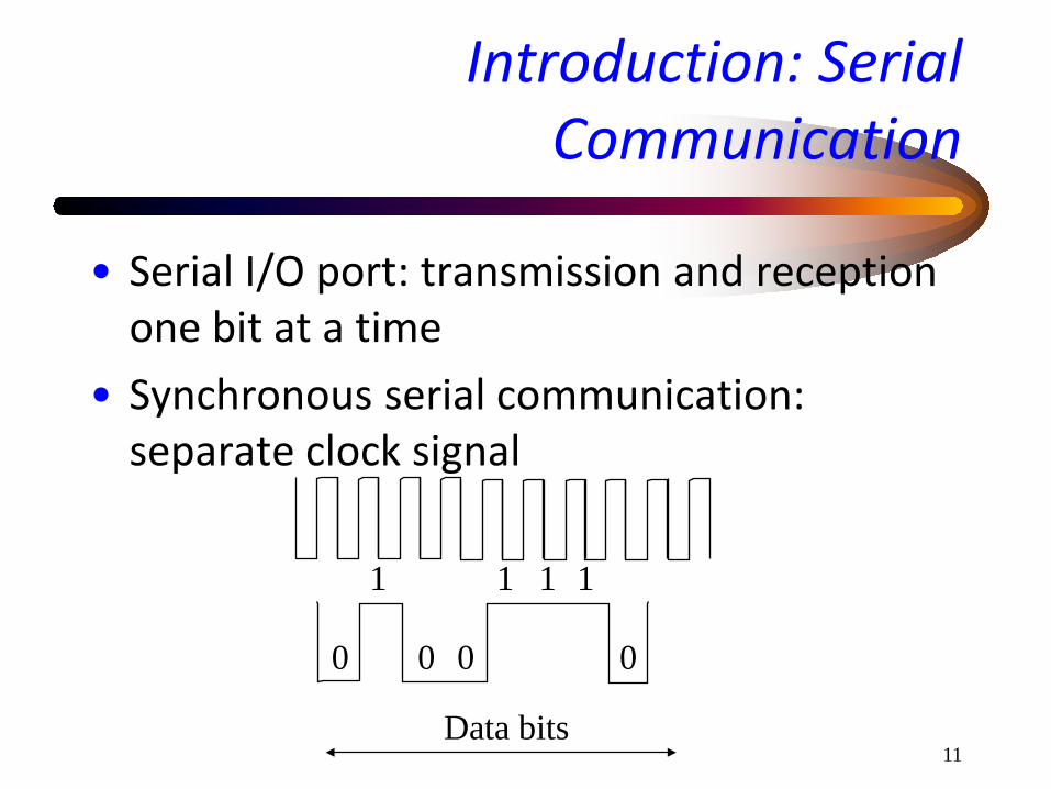
Introduction: Serial Communication
• Serial I/O port: transmission and reception one bit at a time
• Synchronous serial communication: separate clock signal
0
1
0 0
1 1 1
0
Data bits

12
Introduction: Serial Communication
• Asynchronous serial communication – Start/stop/parity bits, baud rate (bits per sec.) – Universal Asynchronous Receiver Transmitter
(UART) – Example of asynchronous serial
communication, 1 start bit, 1 stop bit, 8 data bits, no parity
Start bit
0
1
0 0
1 1 1
Stop bit
0
Data bits

13
Introduction: RS-232
• Voltage level, DB-25, DB-9 connectors, ~20 kbaud (k-bits/sec), 50 ft. Physical-electrical-functional standards.
• As few as 3 pins used. • Null modem or crossover cable: connection
between computers instead of computer to device.
14
Introduction: Plug-in-slots
• Slots: electrical connections to CPU and other parts – Diskette drive, serial port, memory expansion,
data acquisition and control, sound card. – Configuration: interrupt request level (IRQ), I/O
port address, direct memory access (DMA) channels
15
Introduction: Bus
• Bus: – Industrial Standard Architecture (ISA),
Extended ISA (EISA) – The “plug-and-play” concept – Peripheral Component Interconnect (PCI) bus:
• PCI chip between slots and processor, uses registers to store configuration info
• high throughput tasks • No need for jumpers or dip switches and no conflicts

16
Introduction: Bus
• Personal Computer Memory Card International Association (PCMCIA) – Memory and modems for portables. – More devices (Ethernet, SCSI interface, CD-
burners, data acquisition, etc) – Fast access (but recent USB standard offers a
convenient alternative)
• Small Computer System Interface (SCSI): high speed parallel interface bus (daisy chain)

17
Introduction: Computer Languages
• Machine-assembly • BASIC (high-level, interpreter-based, low
storage requirements) • C (high level, transportable, efficient) • MATLAB (and others; C-based-kernel,
arrays, very-high-level math macros inv(A), A*B)
• Simulink: MATLAB GUI, system simulation, block diagram definitions

18
Introduction: Computer Languages
• MATLAB/SIMULINK: expansion via toolboxes (collection of functions written in MATLAB, (or C, Fortran, then converted to an executable .dll or .mex for older versions)
• Recent developments: ability to compile MATLAB code and create stand-alone executables
• xPC, xPC-target: real-time stand-alone applications from SIMULINK code

19
Introduction: Computer Languages
• xPC: Ability to perform rapid prototyping by constructing real-time code with very-high-level GUI. – Good for standard I/O interfacing – Easy-to-maintain code (SIMULINK) – More complicated applications may require the
development of new interface drivers – More info: on-line or web help from mathworks

20
Introduction: MATLAB
• MATLAB: Initially, computations with arrays e.g., A*b, A\b, eig(A), svd(A). Then expanded to address all “signal and system” topics.
• Basic file structure: – m-files: scripts or functions, with high level
interpreter commands – mat-files: data in binary format (see LOAD/SAVE)
– .dll: executable code

21
Introduction: MATLAB
• Other commands – “help:” the most important command… – Commands for systems, control, signal
processing, image processing, neural networks, … – arranged in “toolboxes”, i.e. directories with m-
files • tree structure is only important for indexing and help but not for
operation • Matlab will only look in the defined “path” for functions and data. A
useful trick is to copy a shortcut in each data directory having an empty option at “Start in”. Then, double click the shortcut to open a MATLAB session and include the current directory in the path.

22
Introduction: MATLAB
• SIMULINK: MATLAB GUI to define simulation systems in block-diagram form – mixed continuous and discrete time, but not as “easy”
as it used to be… – .mdl files contain an ASCII description of the
parameters of each block – s-functions: key building block of the simulator, relying
on the concept of the state; fairly easy to create custom blocks but becomes complicated if real time executables are created

23
Introduction: MATLAB
A SIMULINK example with:
A main block (Furnace emulator),
RS-232 I/O, Analog I/O, and Screen output More details in Furnace Notes.doc

24
Typical Configuration of a data acquisition and control system
digital signal
Transducer Signal
Conditioning (Amplify/Filter)
ADC
physical quantities
analog electrical
signal
uProcessor DAC Actuator
process output
process input

25
Computer Interfacing for Data Acquisition and Control
• Data acquisition: discretization in time and quantization in state-space
• Sampling theorem, Nyquist frequency. – No-aliasing condition: Tsample = 1/(2 fmax) – Practical selection: Tsample = 1/(20fmax) – Use of anti-aliasing filters (Review!)
• Quantization resolution = full scale/2n

26
Digital Signals
• PLC (Programmable Logic Controllers): well suited for Boolean Algebra implementations – E.g., Alarm when
• low level and high pressure • high level and high temperature • high level and low temperature and high pressure
– Analog implementation of a two-level signal with hysteresis: op-amp with positive feedback
27
Digital Components
• TTL, CMOS – Digital logic circuits will not drive actuators
directly
• Electromechanical or solid-state relays – Switch high currents and voltages – Considerations: wear, corrosion, arcing,
robustness, speed, noise immunity
• Encoders, counters, latches, tri-state buffers

28
Analog Circuitry
• The 4-20mA standard: current signal information ranging between 4 and 20mA. – 4mA minimum to check integrity, 20mA
maximum to indicate malfunctions – can drive various instrumentation devices with
standardized input – many actuators follow the same standard and
work with 4-20mA inputs – 3-15psi (20-100kPa) pneumatic loop standard
29
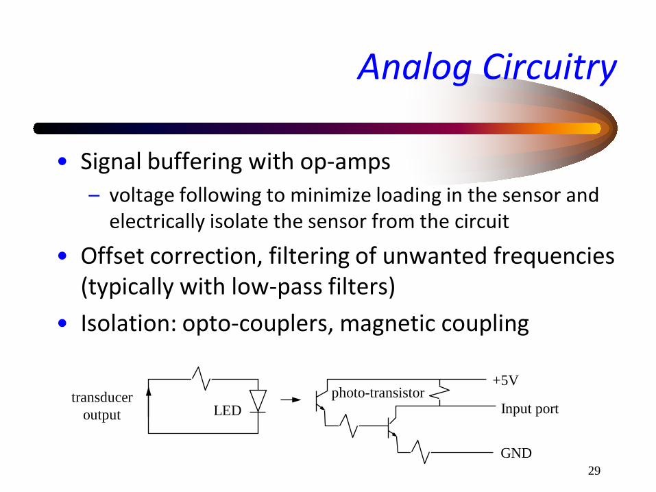
Analog Circuitry
• Signal buffering with op-amps – voltage following to minimize loading in the sensor and
electrically isolate the sensor from the circuit
• Offset correction, filtering of unwanted frequencies (typically with low-pass filters)
• Isolation: opto-couplers, magnetic coupling
transducer output LED
photo-transistor
GND
Input port
+5V

30
Analog Circuitry
• Op-amps:
– Active filters, low-pass, high pass, notch, etc. – Voltage followers (high input impedance, low
output impedance) – Summation, difference, current-to-voltage
conversion, voltage-to-current conversion – Nonlinear function inversion (when Zo = diode
(exponential, ) => logarithmic amplifier
Zo Zi Vin
ZZVout
i
o−=
oaVei =
31
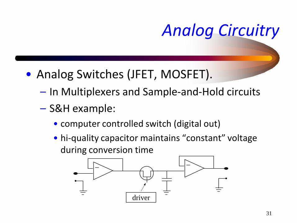
Analog Circuitry
• Analog Switches (JFET, MOSFET). – In Multiplexers and Sample-and-Hold circuits – S&H example:
• computer controlled switch (digital out) • hi-quality capacitor maintains “constant” voltage
during conversion time
driver

32
DAC-ADC
• DAC – “Binary ladder” networks (requires large resistances) – “R-2R ladder” network
R
Vref
R R
2R
2R
(110)

33
DAC-ADC
• ADC – Counter or ramp (slow, 2n cycles) – Dual slope (noise averaging, slow) – Successive Approximation (fast, n cycles)
Successive Approximation
Register
DAC Digital out
Vin C Comparator out

34
Quantization
• A special type of error: uncertainty reduction but with reduced accuracy
• 12-bit A/D, 0-5V =>5/212 =1.2mV resolution • Model of the quantization process
• Signal conditioning: Scaling to full range
quantization <=> x xq x
n xq
n: random noise, uniform
distribution [-1/2n+1, 1/2n+1]

35
Quantization
• Need for scaling: – Temperature range 0-2000oC. Thermocouple
output 0-30mV (assumed linear). 12bit A/D, 0-5V. Resolution: 1.2mV (from before) ~ (2000/30m)*1.2m = 80 oC => measurement = value +/- 40oC!
– Amplify TC measurement by 5/0.03 = 166.67. Resolution: (2000/5)*1.2m = 0.48 oC (reasonable)

36
Quantization II
• Quantization issues in Filtering and Control – Finite precision introduces errors in the computations as well
as in the filter implementation. – Fixed-point arithmetic: bounded noise – 3 classes of errors:
• 1. A/D conversion: Type 1 errors due to signal quantization. Typical error is 1/2 LSB
• Multiplication: Type 2 errors due to signal quantization and truncation. Loss of several LSBs
• Coefficients: Type 3 errors due to finite wordlength in filter implementation. Can cause filter instability. More important in FeedForward control.
quantization <=> x
xq
x n
xq
n: random noise, uniform
distribution [-1/2n+1, 1/2n+1]

37
Quantization II
• Type 1 and 2 quantization errors – Modeled as independent random noise with uniform
distribution. – Error analysis: Compute the overall transfer function H(s) from
the quantization error(s) “q” to the output of interest “e” and use an appropriate metric to quantify the effect of q on e 1. Maximum error bound (very conservative) 2. RMS error bound (usually conservative) 3. Variance (good estimate, most appropriate for this case) Note: The conservatism of the estimate does not mean that the metric is
not important, just that the analysis is not tight.
H(s) q e
38
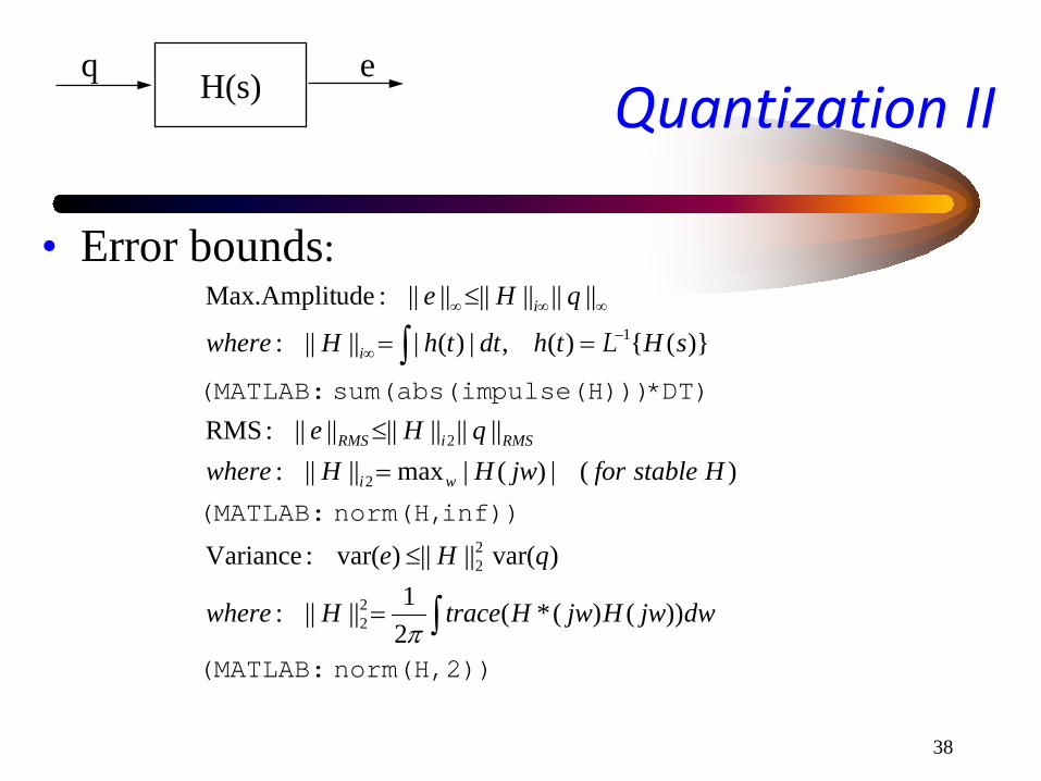
Quantization II
• Error bounds:
H(s) q e
norm(H,2)) (MATLAB:
inf))norm(H, (MATLAB:
DT)*pulse(H)))sum(abs(im (MATLAB:
∫
∫
=
≤
=≤
==
≤−
∞
∞∞∞
dwjwHjwHtraceHwhere
qHe
HstableforjwHHwhereqHe
sHthdtthHwhere
qHe
wi
RMSiRMS
i
i
))()(*(21||||:
)var(||||)var(:Variance
)(|)(|max||||:||||||||||||:RMS
)()(,|)(|||||:
||||||||||||:udeMax.Amplit
22
22
2
2
1
π
L

39
Quantization II
• Example: – Consider the plant P(s)=1/s, with the controller C(s)=(s+1)/s.
Analyze the effect of a 10-bit input quantization on the output. – Discretization interval 0.01s, ZOH – H = P/(1+PC) = s/(s2+s+1) – Hd = 0.01(z-1)/(z2-1.99z+0.9901) – CT:t=[0:.001:50]';h=impulse(H,t);plot(t,h);Hii=sum(abs(h))*.001
– Hii =1.306, Hi2 = norm(H,inf) = 1, H22 = norm(H,2) ^2 = 0.5 – DT:k=[0:10000]';h=impulse(Hd,k*.01);plot(k,h);Hii=sum(abs(h))
– Hii =1.3181, Hi2 = norm(H,inf) = 1.0044, H22 = norm(H,2) ^2 = 0.0051
H(s) q e
40
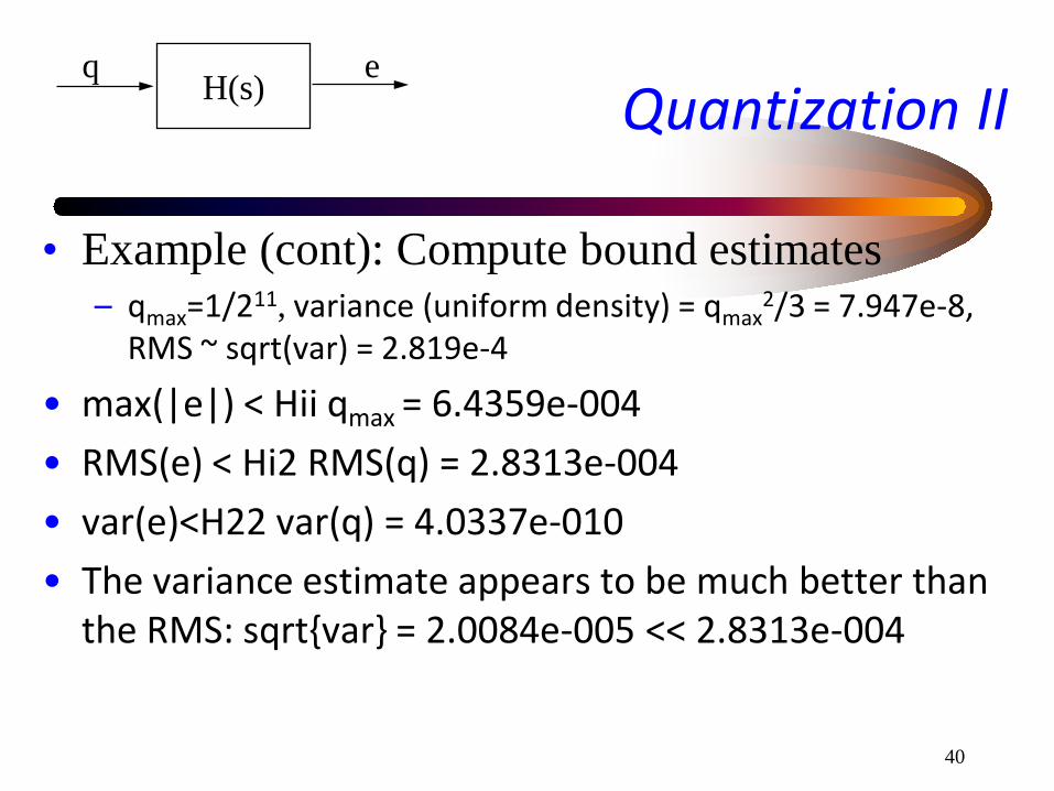
Quantization II
• Example (cont): Compute bound estimates – qmax=1/211, variance (uniform density) = qmax
2/3 = 7.947e-8, RMS ~ sqrt(var) = 2.819e-4
• max(|e|) < Hii qmax = 6.4359e-004 • RMS(e) < Hi2 RMS(q) = 2.8313e-004 • var(e)<H22 var(q) = 4.0337e-010 • The variance estimate appears to be much better than
the RMS: sqrtvar = 2.0084e-005 << 2.8313e-004
H(s) q e

41
Quantization II
• Example (cont): Evaluate the estimates by simulation
• qm=1/2^11 ;q=(rand(10000,1)-0.5)*2*qm;k=[0:10000-1]';subplot(121),plot(k,q), title('q vs sample')
• Hd=fbk(c2d(P,.01),c2d(C,.01)),e=lsim(Hd,q);subplot(122),plot(k,e),title('e=H[q] vs sample')
• [max(abs(e)),sum(abs(h))*max(abs(q))] = 6.2659e-005 6.4352e-004 • [rms(e),norm(H,inf)*rms(q)] = 1.9416e-005 2.7953e-004 • [var(e),norm(H,2)^2*var(q)] = 3.7701e-010 3.9322e-010
H(s) q e

42
Quantization II H(s) q e
• Comments: • The max abs estimate is conservative by an order of magnitude. • The var estimate is much better than the RMS. • However, from the theory we know that the RMS bound is tight. The
apparent discrepancy is due to the fact that var is defined for stochastic signals and RMS^2 is just its estimate from one realization. The variance estimate is good for stochastic inputs only and it is not an upper bound for deterministic signals as the next computation shows:
– z=sin(.01*k); y=lsim(H,z); – [rms(y),norm(H,inf)*rms(z)]=7.0490e-001 7.1171e-001 – [var(y),norm(H,2)^2*var(z)]=4.9686e-001 2.5490e-003 – Notice that norm(H,2)^2*var(z) is NOT a bound on var(y) any more! – But the bound norm(H,inf) *rms(z) on rms(y) is now tight.

43
Quantization II
• Quantization issues in Filtering and Control – Due to the sensitivity of roots of polynomials to perturbations,
the quantization of the filter coefficients can result in a different, possibly unstable filter
– Different filter realizations can be more or less susceptible to quantization problems (parallel or cascades of 1st or 2nd order are preferred over direct forms)
– Problems become more pronounced as the sampling rate increases (the discrete poles accumulate around 1 and there is loss of resolution)

44
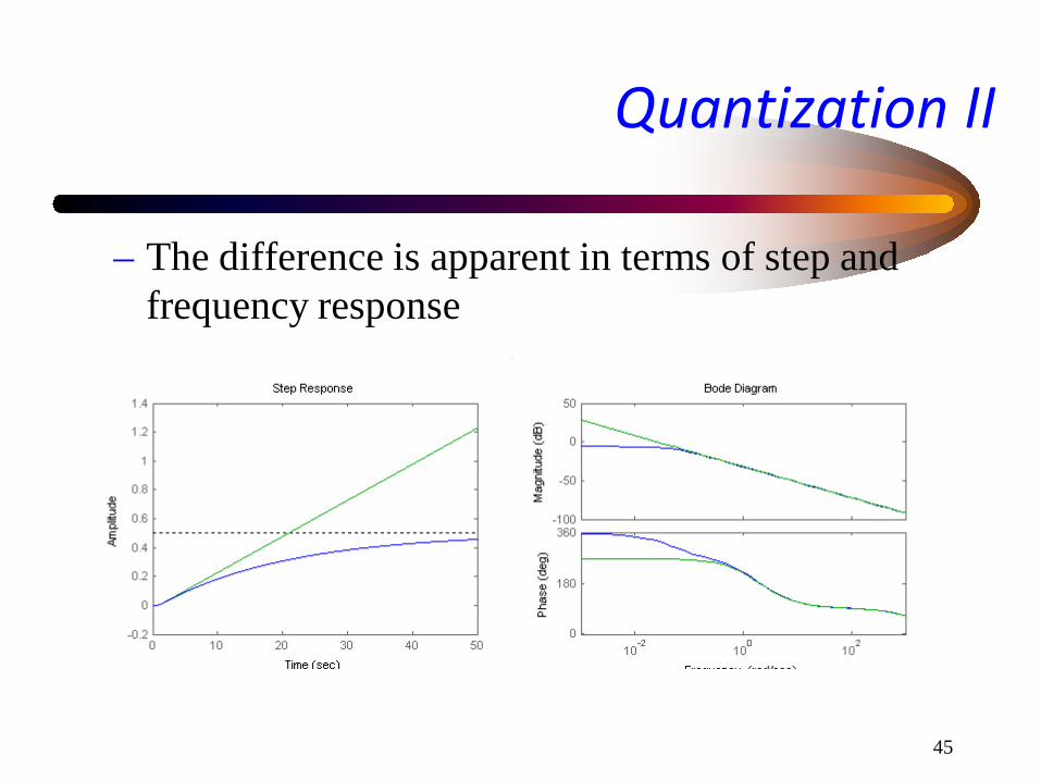
• Example – Start with the heated-water-tube transfer function – P=tf([-.5 1],[.5 1])*tf(1,[40 2]) – Discretize: PD=c2d(P,.001) – Enter the same transfer function with 4 significant digits:
PD2=tf([-2.495e-5 2.5e-5],[1 -1.998 .998]) – The first is stable with poles 9.9995e-00, 9.9800e-001 – The second is unstable with poles 1.0000e+000, 9.9800e-
001
Quantization II
45
– The difference is apparent in terms of step and frequency response
Quantization II
46
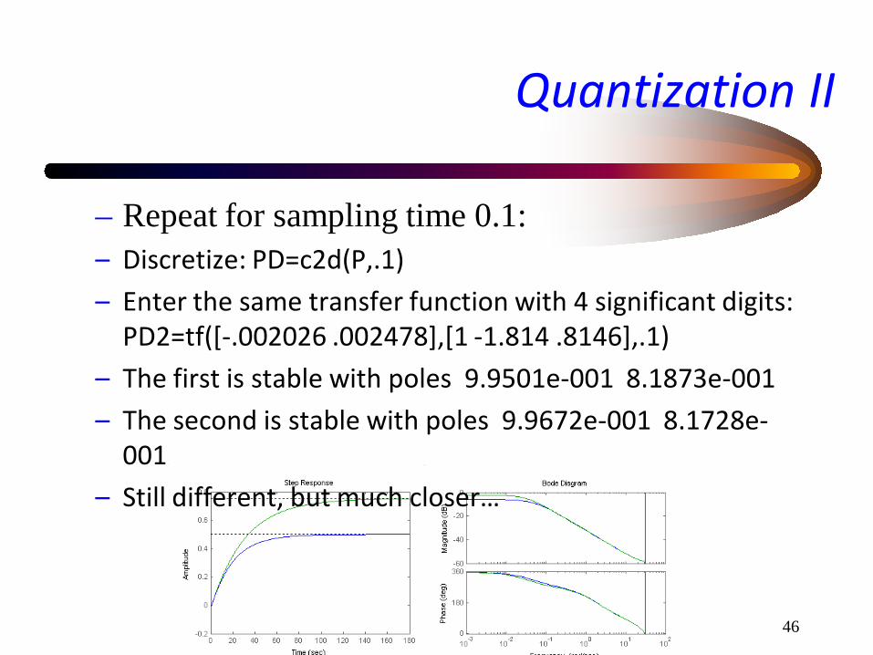
– Repeat for sampling time 0.1: – Discretize: PD=c2d(P,.1) – Enter the same transfer function with 4 significant digits:
PD2=tf([-.002026 .002478],[1 -1.814 .8146],.1) – The first is stable with poles 9.9501e-001 8.1873e-001 – The second is stable with poles 9.9672e-001 8.1728e-
001 – Still different, but much closer…
Quantization II

47
Quantization II
• Some insight – roots of 2nd order polynomial whose coefficients,
are quantized to 0.1

48
Cables
• Flat cables: 1-10V, 100mA • Twisted pair, shielded or unshielded • Coaxial (less interference but not too
popular) • Digital connections, cheaper for low data
rates • Buffering (amplifying) and latching, for
signals on a bus

49
Data acquisition and control with standard add-on cards
• Multifunctional cards: A/D, D/A, digital I/O, counter/timer operations – 4-16 multiplexed A/D, 1-2 D/A, (max rate quoted
for all channels combined) – programming commands (in C or high-level)
• Industrial signal conditioners – thermocouple linearization and cold junction
compensation, filtering and amplification, strain gauge linearization, etc.

50
Data acquisition and control with standard add-on cards
• Signal Conditioning Extensions for Instrumentation (SCXI): high performance system for use with PCI
• Remote I/O modules. Standard RS-232, RS-485 interfaces for 15-bit measurement resolution
• IEEE-488 GPIB (general purpose interface bus) – rigidly defined, 1Mbyte/s transfer rates, multiple
(15) devices to a single network

51
Data acquisition and control with standard add-on cards
• IEEE-488 GPIB hardware specs – total cable length 20m, individual device cable 2m – 24 lines in the cable, clearly defined; 8 data, 8
handshaking, 8 grounding and shielding – star, daisy chain, mixed networks
• GPIB devices – Talkers, listeners, controllers; interconnected via
back plane.

52
Data acquisition and control with standard add-on cards
• Backplane Bus – Board on which connectors are mounted;
provides data, address, control signals
• STE Bus – 8 bit, 20 address lines (1MB memory), 4kB
addressable I/O – Compact cards, robust two part connector, shock
and vibration resistant – IEEE-1000 standard

53
Data acquisition and control with standard add-on cards
• VME Bus – Motorola design for the 32 bit 68000-based system. – 24MHz data transfer rate – 32 bit address bus
• VXI Bus (VME extension for instrumentation) – Improvement over GPIB in communication speed,
synchronization and triggering – Various possible system configurations including GPIB
54
Microcontrollers
• Microprocessors with analog and binary I/O, timers, counters, to perform real-time control functions (8, 16, 32 bit) – Characteristics: 4kB ROM, 128B RAM, single byte
instructions, built-in counters, timers, I/O ports – Intel 8051, 8096, Motorola MCH68HC11, etc. – DSP (Digital Signal Processors): special
architecture for high speed numerical tasks. Separate data bus from instruction bus.

55
Microcontrollers
• The Arduino family – Inexpensive evaluation boards (low-medium
capabilities) – Available drivers making their programming easy
(albeit with some restrictions) – Large development forums (software and 3rd
party hardware support)

56
Distributed Digital Control Systems
• Increased complexity is less of an issue • Additional functions over older analog systems
(redundancy, failure detection, communication, data storage, adaptation/scheduling)
• Overall more reliable, less susceptible to computational noise, controllers are not degrading with time
• Low cost

57
Distributed Digital Control Systems
• Process control applications – Plant automation – Programmable logic controllers (PLC, sequencing jobs) – Regulatory process control: single loop PID or Distributed
Control System (DCS) for large-scale applications – Batch processes: repetitive nature; “run-to-run”
optimization schemes – Advanced applications (identification and control)
58
Distributed Digital Control Systems
• Computer networks, different topologies – For control over networks, the issues of
reliability, and deterministic message transmission must be addressed
– Network communications: common modular set of rules for generating and interpreting messages
– Open System Interconnection (OSI): 7-layer architecture; Physical, Data link, Network, Transport, Session, Presentation, Application

59
Distributed Digital Control Systems
• OSI components – Repeater, at the physical layer – Bridge, at data link layer – Router, at network layer – Gateway, at higher levels
• Communication protocols define connectors, cables, signals, data formats, error checking, algorithms for network interfaces and nodes

60
Distributed Digital Control Systems
• Communication protocols – Simple: polling and interrupt driven – Token ring and Token Bus – Carrier sense multiple access with collision
detection (CSMA/CD) • IEEE 802.3. Check for network activity. If idle, a node
may transmit, then the network becomes busy. In case of collision, transmission is aborted and a random wait time is introduced.

61
Distributed Digital Control Systems
– CSMA/CD • Simple algorithm, non-deterministic, priorities not
supported, collisions a problem at high network loads, analog technology for collision detection
• Ethernet is an implementation of CSMA/CD network. 10Mb/s, coaxial cable or twisted pair. E.g., National Semiconductor 3-chip implementation: Network interface controller (protocol, information movement), Serial network interface (clock), Coaxial transceiver interface (coaxial versions)
– Token ring and Token Bus

62
Distributed Digital Control Systems
• Several DCS platforms from major manufacturers – Honeywell, Foxboro, Fisher and Porter,
Westinghouse, EMC control, Reliance Electric, Beckman Instruments
• Recently, PC or workstation based systems, supervising local embedded controller boards

63
Examples of Computer Control
• Industrial processes versus laboratory experiments
• Several aspects: – Process description and modeling – Sensors and actuators – Controller design (algorithm and structure) – Discretization and implementation – Auxiliary functionality

64
Examples of Computer Control
• Liquid level system – Tank - valve - pump in different configurations – Differential pressure transducer (translating to
level). Other options: floaters, resistivity measurements.
– Valve as a final control element (with or without a pump). Electric valve, pneumatic valve (common), electric actuation via I/P current-to-pressure converter
65
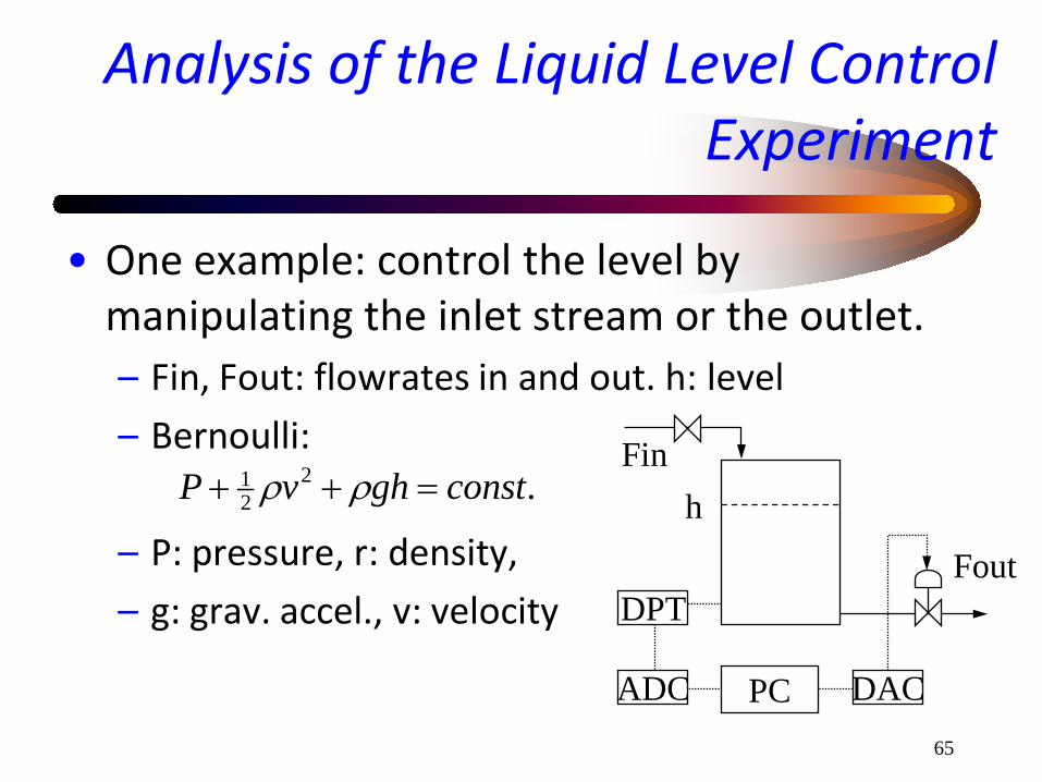
Analysis of the Liquid Level Control Experiment
• One example: control the level by manipulating the inlet stream or the outlet. – Fin, Fout: flowrates in and out. h: level – Bernoulli:
– P: pressure, r: density, – g: grav. accel., v: velocity
PC
DPT
DAC ADC
Fin
Fout
h .221 constghvP =++ ρρ

66
Analysis of the Liquid Level Control Experiment
– inlet conditions – incompressible flow – Bernoulli
– simplify
• A = cross section area, inlet-outlet
• “Ideal” flow i
i
o
i
ini
ioinooinii
oioioiooi
oooiii
ooii
outinii
ghAA
AFh
ghAFvAFhA
vghvvAAhPP
ghvPghvP
vAvAFFhA
2
2
2,0, 2
2212
21
−=⇒
−=−=⇒
≅⇒<<⇒>>==
++=++
=−=
ρρρρ
PC
DPT
DAC ADC
Fin
Fout
h

67
Analysis of the Liquid Level Control Experiment
• ODE for h, nonlinear: slower than linear response for large levels h; faster for small h. – Tank drains in finite time – Addition of a pump: reduced sensitivity of
outflow to liquid level in the tank
• Next, the manipulated variable: We open or close the valve, i.e., we effectively modify the outlet cross section area.
PC
DPT
DAC ADC
Fin
Fout
h

68
Analysis of the Liquid Level Control Experiment
• Valves – Many types with different characteristics (pressure drop,
open/close speed, size, linearity, sealing). – Ball (common, e.g., manual/auto sprinkler valves at the
store)
– Gate (sliding in and out to restrict flow) • easier to compute cross section area
Ball, side and front view (spherical housing not shown)
Disc-shaped Gate, front view
PC
DPT
DAC ADC
Fin
Fout
h
69
Analysis of the Liquid Level Control Experiment
• Let us select a gate valve with a motorized screw as an opening/closing mechanism.
• We manipulate the current to the motor or, in a high friction simplification, the motor speed. – Suppose that at max speed, it takes 2 sec from full-open
to full-close
• Other options: Manipulate the set-point of a valve controller, for a %-open value; pneumatic valves with a I/P converter.
PC
DPT
DAC ADC
Fin
Fout
h

70
Analysis of the Liquid Level Control Experiment
• Compute cross section area as a function of %-open (distance between gate center and pipe center) – shaded area = 2x[sector - triangle area] –
– Relation to control input:
( ) ( )
( )[ ] rdDDDDrA
drlldAREATRIANGLEr
drAREASECTORrd
o 2,1cos2
4,4/.2cos.,2cos
212
22
121
=−−=⇒⇒
−==
==
−
−−
θd
r
2θ
l
ud =
PC
DPT
DAC ADC
Fin
Fout
h
71
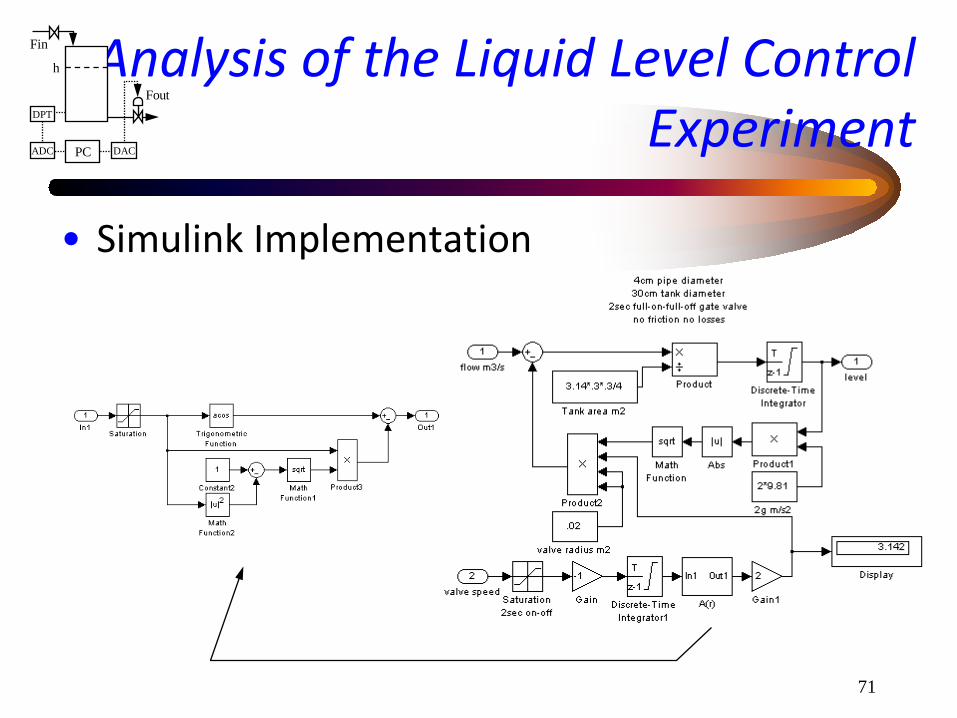
Analysis of the Liquid Level Control Experiment
• Simulink Implementation
PC
DPT
DAC ADC
Fin
Fout
h
72
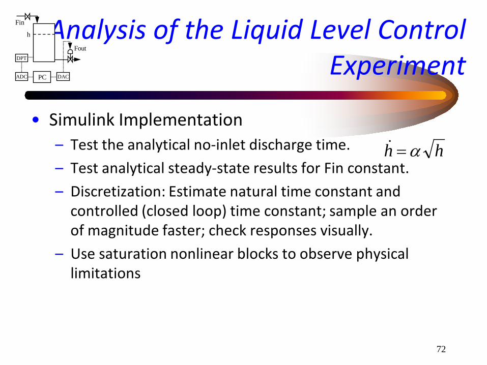
Analysis of the Liquid Level Control Experiment
• Simulink Implementation – Test the analytical no-inlet discharge time. – Test analytical steady-state results for Fin constant. – Discretization: Estimate natural time constant and
controlled (closed loop) time constant; sample an order of magnitude faster; check responses visually.
– Use saturation nonlinear blocks to observe physical limitations
hh α=
PC
DPT
DAC ADC
Fin
Fout
h
73
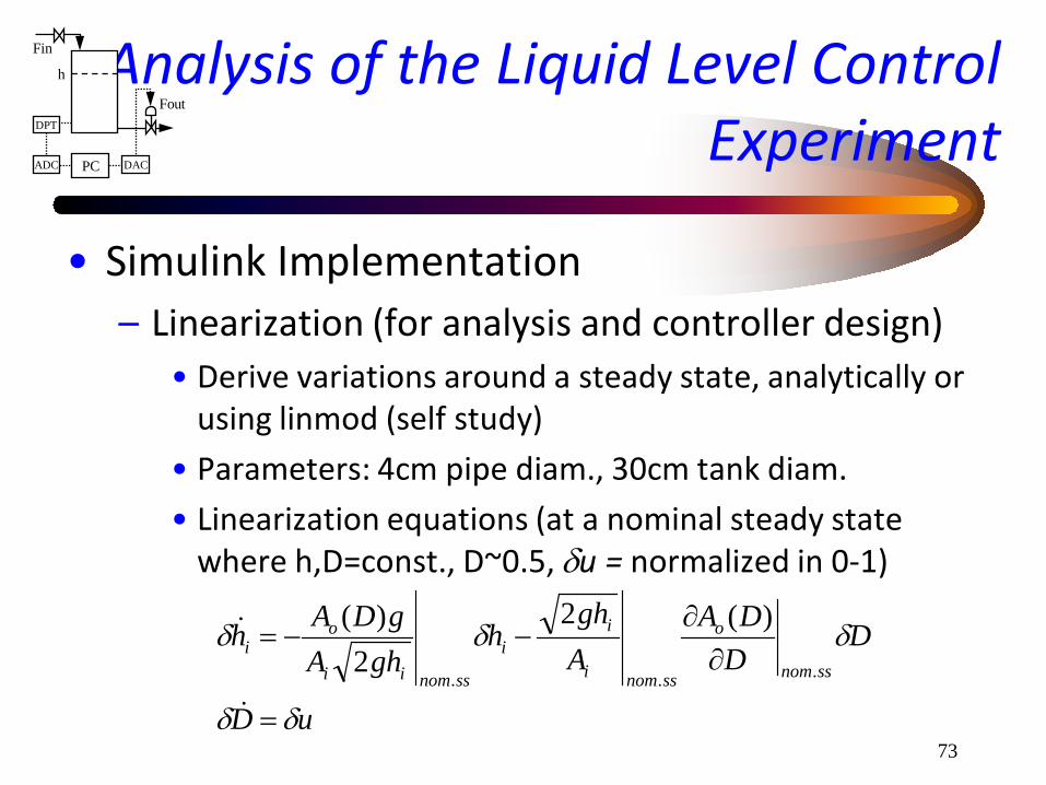
Analysis of the Liquid Level Control Experiment
• Simulink Implementation – Linearization (for analysis and controller design)
• Derive variations around a steady state, analytically or using linmod (self study)
• Parameters: 4cm pipe diam., 30cm tank diam. • Linearization equations (at a nominal steady state
where h,D=const., D~0.5, δu = normalized in 0-1)
uD
DDDA
Agh
hghA
gDAhssnom
o
ssnomi
ii
ssnomii
oi
δδ
δδδ
=
∂∂
−−=
...
)(22
)(
PC
DPT
DAC ADC
Fin
Fout
h
74
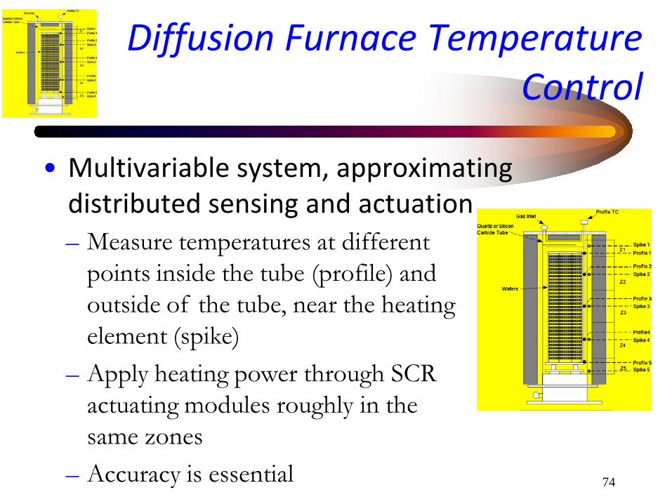
Diffusion Furnace Temperature Control
• Multivariable system, approximating distributed sensing and actuation – Measure temperatures at different
points inside the tube (profile) and outside of the tube, near the heating element (spike)
– Apply heating power through SCR actuating modules roughly in the same zones
– Accuracy is essential
75
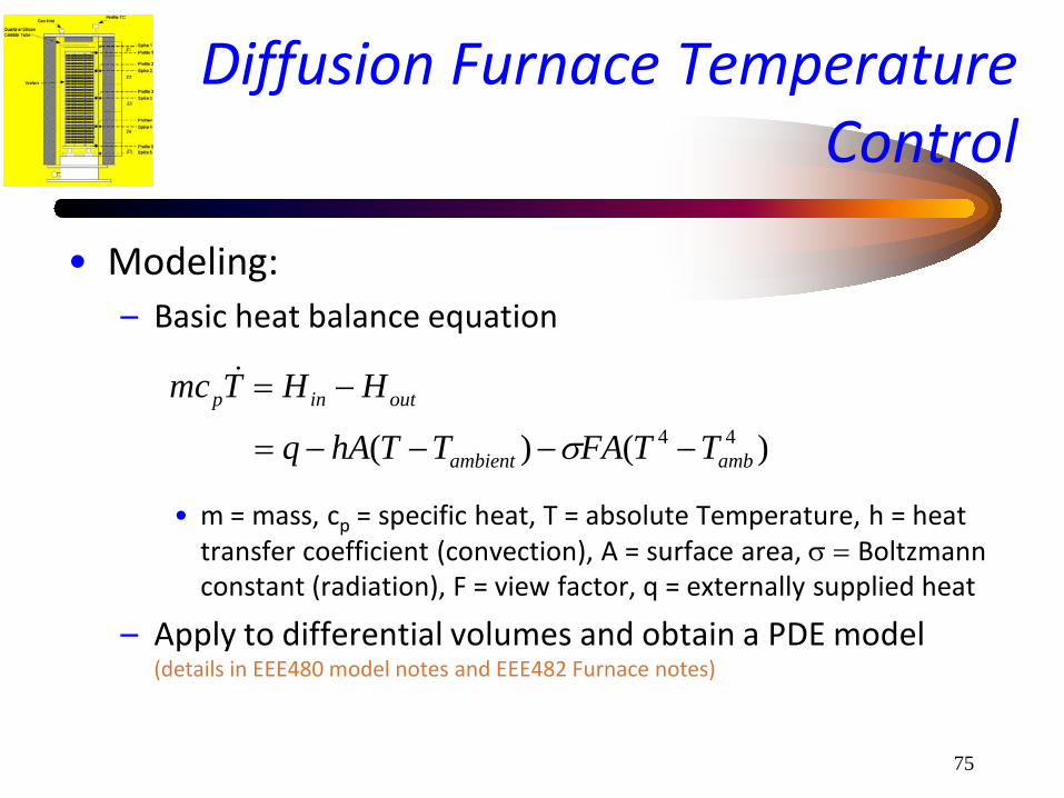
Diffusion Furnace Temperature Control
• Modeling: – Basic heat balance equation
• m = mass, cp = specific heat, T = absolute Temperature, h = heat
transfer coefficient (convection), A = surface area, σ = Boltzmann constant (radiation), F = view factor, q = externally supplied heat
– Apply to differential volumes and obtain a PDE model (details in EEE480 model notes and EEE482 Furnace notes)
)()( 44ambambient
outinp
TTFATThAq
HHTmc
−−−−=
−=
σ

76
Diffusion Furnace Temperature Control
• Sensors: Thermocouples for high temperatures (some operations above 1000deg.C). Pyrometry is another option for single wafer reactors. – Issues: Cold-junction compensation, amplification, and
table look-up linearization. RF interference may appear from SCR application of electrical power
• Actuators: SCR modules – Issues: resolution - switching transient trade-off

77
Diffusion Furnace Temperature Control
• Need for elaborate and precise controllers – Newer furnaces have more (5) heating zones for more
resolution and improved uniformity (temperature coupling is higher than in the older 3-zone furnaces)
– Due to radiation nonlinearity, different controllers may be necessary to cover a big temperature range
– Nonlinearity and coupling are more pronounced in single-wafer rapid thermal processors (RTP), using arrays of heating lamps

78
Diffusion Furnace Temperature Control
• Controller communications Thermocouples
Analog conditioning, amplification
Embedded controller ADC, linearization, (PID), DAC
Network Communication
Heating elements
SCR Firing board
Network: Monitoring stations, Data storage
Recipe management
ethernet Advanced controller
computations real time comm. e.g., RS232,
backplane bus PC104 bus…

79
Control of Paper Machines
• Process description
• K. Tsakalis, S. Dash, A. Green, and W. MacArthur, “Loop-Shaping Controller Design From Input–Output Data: Application to a Paper Machine Simulator,” IEEE TRANSACTIONS ON CONTROL SYSTEMS TECHNOLOGY, VOL. 10, NO. 1, 127-136, JANUARY 2002

80
Control of Paper Machines
• Control Inputs (manipulated variables) – stock flow (solids), dryer temperatures (as set points to local PID
loops), machine speed (as set point to drum motors)
• Process Outputs (controlled variables) – paper dry weight (~solids), Moisture content (at different points),
machine speed (actual)
• Disturbances – Operators can change set-points in other loops to maintain the
overall product quality. Feed consistency is a major disturbance, especially after paper breaks (re-circulation).

81
Control of Paper Machines
• Challenges in Paper Machine control – Consistency control (in the direction of production) – Cross-directional control (across the paper; distributed
control, not discussed here) – Interacting variables, wide range of process responses.
Standard decoupled single-loop control not very effective – E.g., Stock/Weight has long dead-time, short settling time,
Steam/Moisture has short dead-time and long time constant, Machine Speed has minimal dead-time and fast dynamics. These features can have an adverse effect on both the identification and the robust control of a paper machine.

82
Control of Paper Machines
• Some ballpark numbers: – Total length of paper line ~500–1000m, speed 10–30 m/s
(20–60 mi/h), dryer drums 2–3 m diam. – Sensors scan moisture and dry weight across the width of
the paper. Scanning interval can be as large as 35 s. – Steam/moisture dynamics
• ~temperature response of the drums (local PID control, closed-loop time constant in the order of a few minutes)
• Short time-delays (scanners, drum-sensor distance), but larger delays for reel moisture (measured at the end of the line)
• “Noise” from the interaction of the paper sheet with the environment
83
Control of Paper Machines
– Stock flow/dry weight dynamics • Larger delay since the actuator is located at the beginning of the
line • Quick settling time, essentially determined by the stock mixing
process • Any changes in the stock flow also have a significant effect on
moisture, since it changes the net water content of the paper sheet • Changes in the drum temperatures or moisture leave the dry
weight unaffected
– Machine speed • Can be controlled much faster than the other variables. Unaffected
by steam or stock flow variations, but it has a significant effect on moisture and dry weight.
84
Heat Exchanger Control Example
• Multivariable system (see textbook), both feedback and feedforward control – Measure inlet temperatures and water outlet
temperature (controlled variable) – Manipulate steam inflow, water inflow through
pneumatic valves – Water flow is a controlled variable, either to be
maximized or to track a setpoint – Other valves and instruments to enable monitoring and
ensure integrity

85
Plastic Injection Molding Process
• Multivariable system, approximating distributed sensing and actuation (see textbook) – Measure temperatures at different points – Apply heating power through SCR actuating
modules at the same points – Accuracy is important
86
Other Control Examples
• Aerospace applications – high performance fighter aircraft, helicopters, jet engines
• Electromechanical systems – robotic arms, pendulum, cart and pendulum
• Automotive – intelligent vehicle highway systems, platooning, traffic
control – engine management, anti-lock brakes, active suspension
• Manufacturing processes, scheduling of operations

87
Feedback and Feedforward Control
• Controller Design Procedure: – Determine inputs and outputs – Model or identify the system – Define the control objectives and specifications – Design the controller (algorithm and parameters) – Discretize (if working in continuous time), quantize and
implement (code + hardware) – Anti-windups and other nonlinear modifications:
integrated (recent methods) or “post-mortem”
P C
Hu
F
y u r
du dy v
88
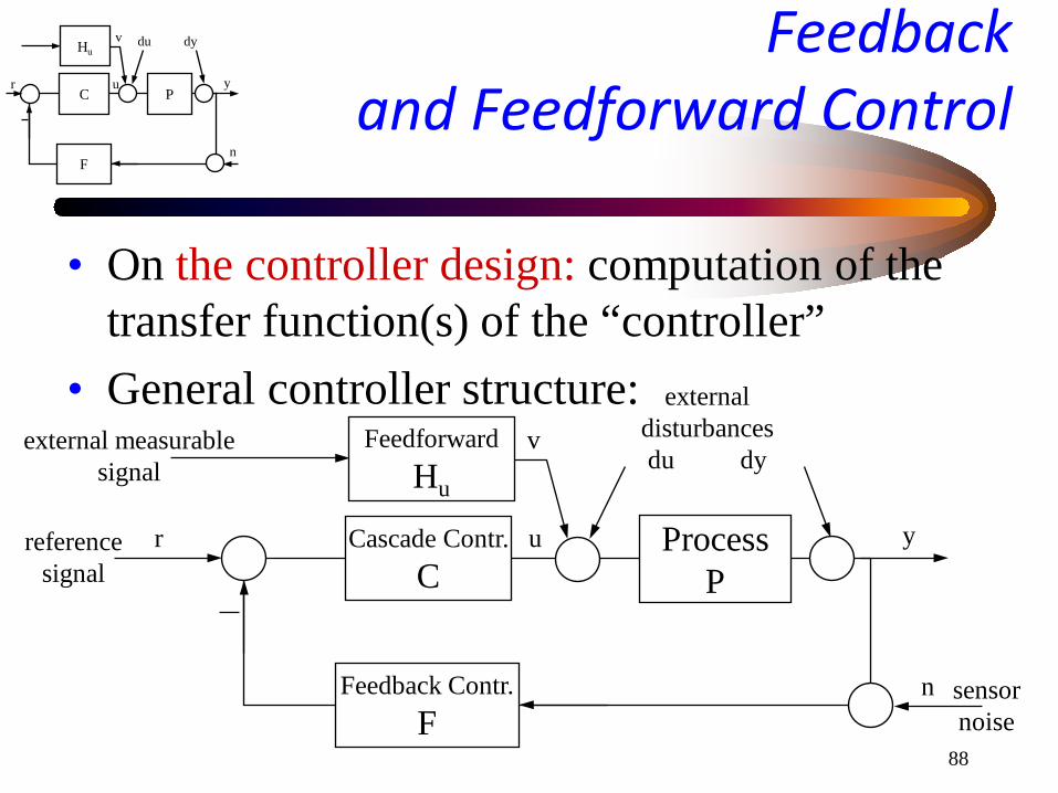
Feedback and Feedforward Control
• On the controller design: computation of the transfer function(s) of the “controller”
• General controller structure: Process
P Cascade Contr.
C
Feedforward Hu
Feedback Contr. F
external measurable signal
y reference signal
sensor noise
u r
external disturbances du dy
v
n
P C
Hu
F
y u r
du dy v
n

89
Feedback and Feedforward Control
• Feedback control objective: Reduce the effect of disturbances on the output
– the disturbance contributions decrease when S is smaller, i.e., when CF is larger
– the noise contribution decreases when CF is smaller
P C
Hu
F
y u r
du dy v
n
)()1(
]][[
][
1 ySensitivitPCFSwhere
SPvSPdSPCFnSPCrSdPvPdnyFrPCd
vduPdy
uy
uy
uy
−+=
++−+=
++−−+=
+++=

90
Feedback and Feedforward Control
• Feedback controller design: – stable loop
• PCF must produce a stable loop (crossover frequency characteristics)
– large gain (magnitude) in the region where the sensor is reliable
• in the same vein, respect uncertainty-imposed constraints (avoid excessive peaks/resonances in S)
• can only attenuate disturbances where the sensor information is reliable
P C
Hu
F
y u r
du dy v
n
91
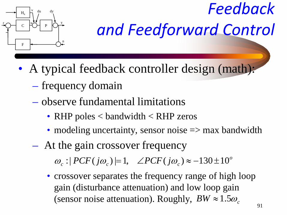
Feedback and Feedforward Control
• A typical feedback controller design (math): – frequency domain – observe fundamental limitations
• RHP poles < bandwidth < RHP zeros • modeling uncertainty, sensor noise => max bandwidth
– At the gain crossover frequency
• crossover separates the frequency range of high loop gain (disturbance attenuation) and low loop gain (sensor noise attenuation). Roughly,
P C
Hu
F
y u r
du dy v
n
occc jPCFjPCF 10130)(,1|)(|: ±−≈∠= ωωω
cBW ω5.1≈

92
Feedback and Feedforward Control
• Feedback controller design: – Software automating most of the computations
• Tuning of PID, robust multivariable, LPV… • Usually, concepts are understood in terms of transfer
functions and in the frequency domain but the computations are performed in the state-space relying on time-domain optimal control theory
• Here: simple PID tuning (Ziegler-Nichols, or pidqtune) – Still, the selection of reasonable objectives is
essential
P C
Hu
F
y u r
du dy v
n

93
Feedback and Feedforward Control
• Feedforward control objective: cancel the effect of a measurable disturbance at the output – General setting:
– If P1 were invertible, H = -P1-1P2
• Usually this is not the case
P1 H y v
P2
m
P1 H y v
P2
m
||||min][
21
2121
PHPmPHPmPvPy
+=>+=+=
94
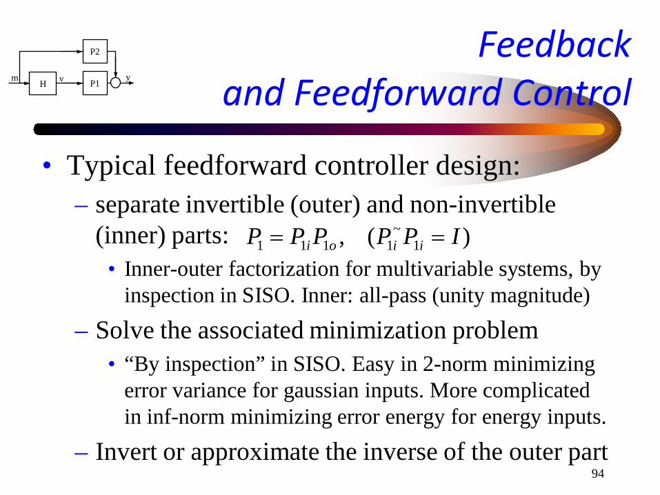
Feedback and Feedforward Control
• Typical feedforward controller design: – separate invertible (outer) and non-invertible
(inner) parts: • Inner-outer factorization for multivariable systems, by
inspection in SISO. Inner: all-pass (unity magnitude) – Solve the associated minimization problem
• “By inspection” in SISO. Easy in 2-norm minimizing error variance for gaussian inputs. More complicated in inf-norm minimizing error energy for energy inputs.
– Invert or approximate the inverse of the outer part
P1 H y v
P2
m
)(, 1~
1111 IPPPPP iioi ==

95
Feedback and Feedforward Control
• Typical feedforward controller design (math) – inner-outer factorization – minimization problem
P1 H y v
P2
m
)(, 1~
1111 IPPPPP iioi ==
Nehari)-(Hinf||||minarg)(:||.||.2
)projection stable-(H2)()(:||.||.1
)1|||| and since(||)(||min
||)(||min||||min
2~
11
1
2~
11
12
~11
~12
~11
21121
∞−
∞
−−
+=
=
==+
=+=+
PPXPHPPPH
PIPPPPHPPHPPPHP
iXo
io
iiiio
oi
)regularizeor weights,add e,approximat (then, defined not well is )( proper,strictly If 1
11−
oo PP

96
Feedback and Feedforward Control
• Example of a (simplified) complete design: – Heating a tube of water, 10liters, 0.1m diameter. – Lumped model
• mcp ~ 40, h=5, A = πDL = 0.4
– Also, suppose that T0 is measurable and there is a 1sec delay in applying the control input (u: q(t) = u(t-1)), modeled by a 1st ord. Pade approximation
P C
Hu
F
y u r
du dy v
n
uhAsmc
dhAsmc
hAy
TdquTyqTThATmc
pp
p
++
+=
===
+−−=
1,,
)(
0
0
97
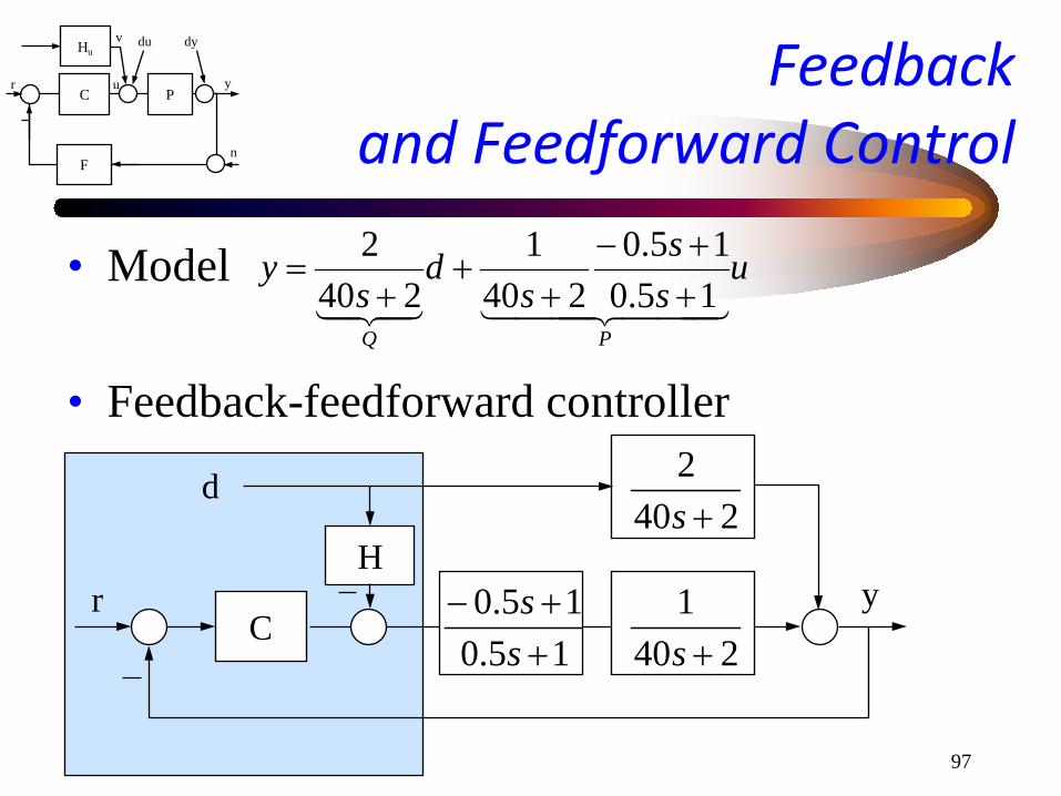
Feedback and Feedforward Control
• Model
• Feedback-feedforward controller
P C
Hu
F
y u r
du dy v
n
uss
sd
sy
PQ 15.0
15.0240
1240
2++−
++
+=
2401+s
2402+s
15.015.0
++−
ss
C
H
d
y r

98
Feedback and Feedforward Control
• Feedback controller tuning: – Choose BW < 2, e.g., 0.2rad/s, (other design
objectives and constraints would be included in this choice) => target crossover 0.2/1.5 = 0.133
– Plant transfer function and frequency response • P=tf([-.5 1],[.5 1])*tf(1,[40 2]) • bode(P)
– phase at crossover: -77o
P C
Hu
F
y u r
du dy v
n

99
Feedback and Feedforward Control
• Feedback controller tuning: – PI controller: C = K(s+a)/s. – Adds phase at crossover: – For 50o phase margin,
– Find corresponding gain K:
• C=tf([1 .1765],[1 0]); bode(P*C) • evaluate magnitude at 0.133 • => K=3.43
P C
Hu
F
y u r
du dy v
n
oa 90)/133.0(tan 1 −−
1765.037)/133.0(tan 1
==>=−
aa o

100
Feedback and Feedforward Control
• Feedback controller tuning: – Final controller: C=tf([3.43 0.61],[1 0]) – Check step response and bandwidth – step(feedback(P*C,1)) -> 23% overshoot – bode(feedback(P*C,1)) -> 0.2 rad/s bandwidth – sampling time < 1/0.2/10, (wT/2 < 0.1) say 0.1s – control signal limits 0-1000(W)
P C
Hu
F
y u r
du dy v
n

101
Feedback and Feedforward Control
• Feedback controller testing: – Test in Simulink
• 50 deg. step. 10 deg., 0.01 Hz disturbance – PI controlled response vs. uncontrolled response
• faster response • disturbance attenuation
P C
Hu
F
y u r
du dy v
n

102
Feedback and Feedforward Control
• Feedforward control – Develop expressions
Subtract the feedforward signal to obtain the standard minimization problem
– Frequency weighting and control penalty
– W=tf([.5 1],[1 1e-4]); rho=1e-3 % This W improves low-frequency performance; the control penalty rho << 1, avoids ill-posed problems; larger values yield smoother controls
P C
Hu
F
y u r
du dy v
n
||)(||min: SQSPHHSQdSPHdSPCry H −=>+−=
−
0
min:WSQ
HI
WSPH H ρ

103
Feedback and Feedforward Control
• Feedforward control computations – S=feedback(1,P*C); SP=feedback(P,C); SQ=Q*S; – % Use the “feedback” function instead of just algebra – G=[W*SP;r]; WT=([W*SQ;0]); – [SPi,SPip,SPo]=iofr(ss(G)); Stil=inv([SPi,SPip]); – R=minreal(Stil*WT); – % Inner-outer factorization, minimal realization to keep system order
low – X2=stabproj(R-R.d)+R.d; H2o=minreal(inv(SPo)*[1 0]*X2); – % Solve the associated net H-2 minimization problem but keep the
throughput R.d in the stable part instead of splitting it (default in “stabproj”)
P C
Hu
F
y u r
du dy v
n

104
Feedback and Feedforward Control
• computations continued – cut=sum((abs(eig(H2o))<1e-2)); – [H2s,H2f]=slowfast(H2o-H2o.d,cut);H2f=H2f+H2o.d; – [a,b,c,d]=h_sysred(H2f,[],[]); H2=ss(a,b,c,d); – % Perform model reduction (the price of generality). “slowfast” to
remove irrelevant slow modes. “h_sysred” is a custom function, based on balanced truncation. Works with the old state-space format.
– % Details in “Stability, Controllability, Observability notes,” http://www.fulton.asu.edu/~tsakalis/notes/sco.pdf
P C
Hu
F
y u r
du dy v
n
105
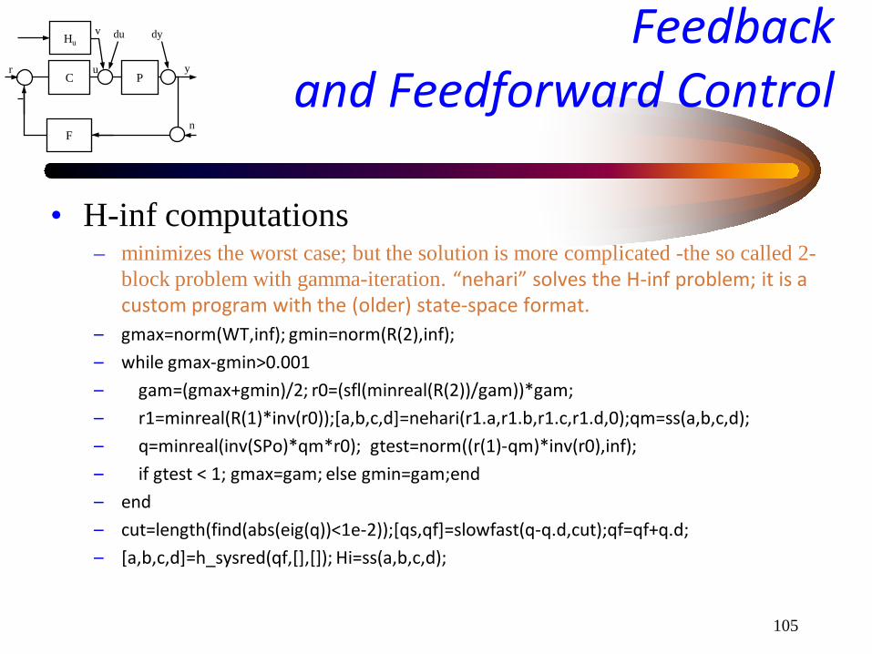
Feedback and Feedforward Control
• H-inf computations – minimizes the worst case; but the solution is more complicated -the so called 2-
block problem with gamma-iteration. “nehari” solves the H-inf problem; it is a custom program with the (older) state-space format.
– gmax=norm(WT,inf); gmin=norm(R(2),inf); – while gmax-gmin>0.001 – gam=(gmax+gmin)/2; r0=(sfl(minreal(R(2))/gam))*gam; – r1=minreal(R(1)*inv(r0));[a,b,c,d]=nehari(r1.a,r1.b,r1.c,r1.d,0);qm=ss(a,b,c,d); – q=minreal(inv(SPo)*qm*r0); gtest=norm((r(1)-qm)*inv(r0),inf); – if gtest < 1; gmax=gam; else gmin=gam;end – end – cut=length(find(abs(eig(q))<1e-2));[qs,qf]=slowfast(q-q.d,cut);qf=qf+q.d; – [a,b,c,d]=h_sysred(qf,[],[]); Hi=ss(a,b,c,d);
P C
Hu
F
y u r
du dy v
n

106
Feedback and Feedforward Control
• Controller Evaluation – Top Fig.: 2nd and full order feedforward filters are
nearly the same – Bottom Fig.: Error transfer function for the 2nd and
full order filters and the obvious choice (without the delay), H=2.
– sigma(SP*2-SQ,SP*H2-SQ,SP*Hi-SQ) – The H-2/H-inf methods produce optimal results
systematically – More pronounced differences for more difficult
problems
P C
Hu
F
y u r
du dy v
n

107
Feedback and Feedforward Control
• Feedforward control implementation – Discretize the filter
• [nu,de]=tfdata(bilin(H2,1,'bwdrec',.1),’v’) • [nu,de]=tfdata(c2d(H2,.1,’tustin’),’v’) • % use “bilin” with ‘bwdrec’ option or “c2d” with ‘tustin’
– Introduce the filter in the Simulink model
P C
Hu
F
y u r
du dy v
n

108
Feedback and Feedforward Control
• Feedback and Feedforward control testing
• No feedforward (blue), • H2 solution (red), • Simple choice H=2 (cyan)
P C
Hu
F
y u r
du dy v
n

109
Feedback and Feedforward Control
• Feedback – Stabilizes or improves stability margin – Reduces sensitivity to unknown perturbations and model
imprecision – Requires good sensors of process output
• Feedforward – Leaves sensitivity and stability unaffected – Provides faster corrections (than feedback) – Requires good models and good sensors of disturbance
P C
Hu
F
y u r
du dy v
n

110
Feedback and Feedforward Control
• Other Design Methods – Feedback
• Linear Quadratic Regulator (LQR) methods • General H2 and Hinf solutions to weighted sensitivity
minimization (more complicated problem statement) • Model Predictive Control (MPC, on-line solution of an
LQR optimization problem) • Other heuristic, optimization-based methods (e.g., PID)
– Feedforward • Heuristic, algebraic
– Discrete-time (sampled data) solutions
P C
Hu
F
y u r
du dy v
n

111
Feedback and Feedforward Control
• References – Anderson-Moore (LQR), – Zhou, Macejiowski (Hx, model reduction, feedforward), – Francis (Hx fundamentals), – McFarlane-Glover (Coprime factor methods) – Glad-Ljung (Linear/nonlinear/MPC… excellent survey) – Astrom (PID control)
P C
Hu
F
y u r
du dy v
n

112
PID Control
• PID Tuning – PID is the industry workhorse
– Proportional, Integral, and Derivative action to achieve all the basic feedback objectives: adjust bandwidth, introduce phase lead for stabilization, increase gain at low frequencies for disturbance attenuation
P C
Hu
F
y u r
du dy v
n
∫ ++=dtdeKeKeKu dip

113
PID Control
• PID Tuning – Pseudo-differentiator: more realistic and avoids
numerical problems in the design
– Transfer function:
P C
Hu
F
y u r
du dy v
n
evvT
veTKeKeKu d
ip
+−=
−++= ∫
)(
)1()()(
1)(
2
+
++++=
+++=
TssKsTKKsTKK
TssK
sKKsC
iippd
dip

114
PID Control
• PID Tuning – Choosing T: minimum value is the sampling time
for discrete implementation. It does not affect the design very much as long as 1/T > 10 BW
– Tuning the PID: choosing the gain and the two zeros in the numerator (the num. is a 2nd degree, arbitrary polynomial, the den. is fixed)
• Typically, the two zeros are chosen the same • PI: a special lag compensator • PD: a lead compensator
P C
Hu
F
y u r
du dy v
n
)1()( 2
++= Tss
asKPIDs
asKPI )( +=
)1()(
++= Ts
asKPD

115
PID Control
• PID Tuning – Classical theory
• phase margin at the intended crossover – Ziegler-Nichols
• Practical methods based on simple models – Optimization and Loop-shaping
• MATLAB custom function “pidqtune” minimizes the distance from a desirable target; target selected using LQR theory so that the closed loop is at least feasible
• files in http://www.fulton.asu.edu/~tsakalis/notes
P C
Hu
F
y u r
du dy v
n
116
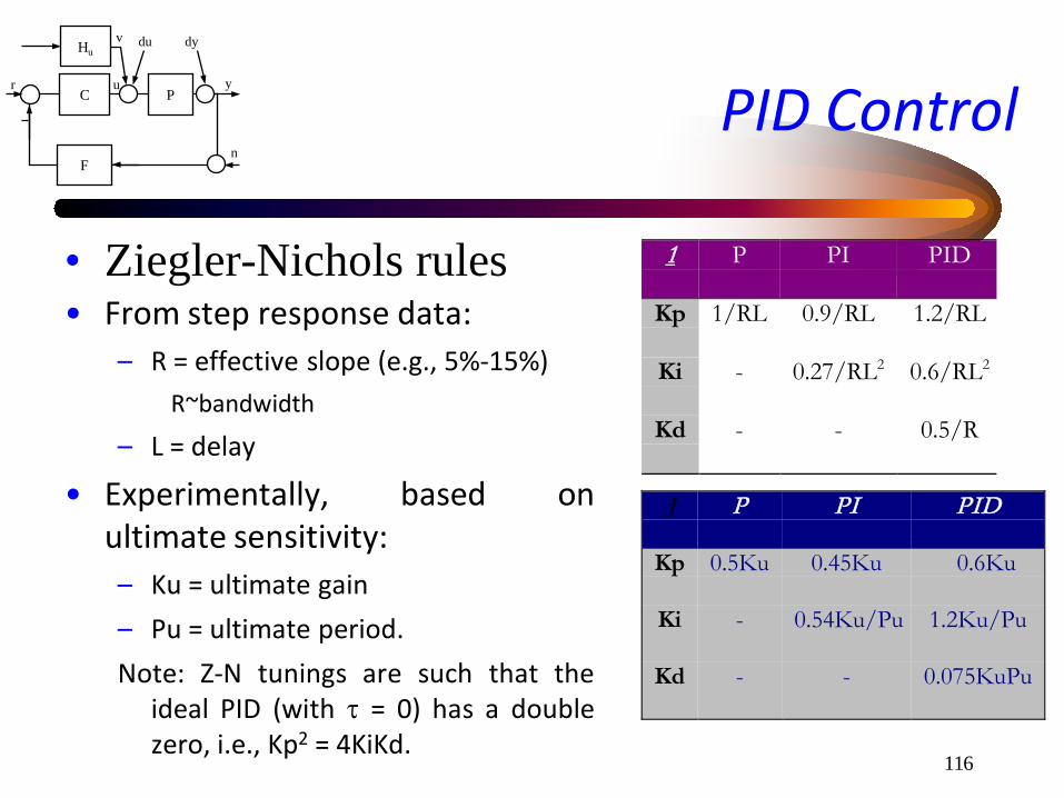
PID Control
• Ziegler-Nichols rules • From step response data:
– R = effective slope (e.g., 5%-15%) R~bandwidth
– L = delay
• Experimentally, based on ultimate sensitivity: – Ku = ultimate gain – Pu = ultimate period. Note: Z-N tunings are such that the
ideal PID (with τ = 0) has a double zero, i.e., Kp2 = 4KiKd.
P C
Hu
F
y u r
du dy v
n
1 P PI PID
Kp 1/RL 0.9/RL 1.2/RL
Ki - 0.27/RL2 0.6/RL2
Kd - - 0.5/R
1 P PI PID
Kp 0.5Ku 0.45Ku 0.6Ku
Ki - 0.54Ku/Pu 1.2Ku/Pu
Kd - - 0.075KuPu

117
PID Control
• PID Discrete Implementation several different but equivalent implementation equations, e.g., – Integrator windup
• Nonlinear behavior when the control input saturates (can lead to instability)
• Remedy: Anti-windup modification (limited integrators)
P C
Hu
F
y u r
du dy v
n
kkk
kkdkikpk
esseeKsKeKu
+=
−++=
+
−
1
1)(
],,min[max maxmin1 ii K
uK
ukkk ess +=+
=−=∆ + kkk uuu 1

118
Controller Discretization
• Discretization
– MATLAB: “bilin” with ‘bwdrec’ (backward
rectangular), ‘fwdrec’, ‘tustin’, etc. – “c2d” function for system objects, with ‘zoh’
(zero order hold) option, etc.
P C
Hu
F
y u r
du dy v
n
BAzICDzGzuzy
DuCxyBuAxx
BAsICDsGsusy
DuCxyBuAxx
kkk
kkk
1
1
1 )()()()()()(
)()(
Time DiscreteTime Continuous
−
+
− −+==
+=+=
−+==
+=+=

119
Controller Discretization
• Discretization derivations
P C
Hu
F
y u r
du dy v
n
TBATIATIzIATICTBATICDTBATIATIzATIzICD
TBzATIATIzICDzG
BuAxT
xxBuAxx
TBATIzICDzG
BuAxT
xxBuAxx
kkkk
kkkk
11111
1111
111
1
1
1
)(])([)(])([)()(])([
)(])([)(
Euler Backward
)]([)(
Euler Forward
−−−−−
−−−−
−−−
−
−
+
−−−−+−+=
−−±−−+=
−−−+=
+=−
→+=
+−+=
+=−
→+=

120
Controller Discretization
• Discretization derivations
P C
Hu
F
y u r
du dy v
n
=⇒
+−
==+−
=
+=−+=→
+=+→+=
−−
−+
+−+∫
...2/12/1,
112
:Tustin
,)(
)()()(
:inputs)constant piecewise with response data (sampled equivalent ZOH
1
11
)(
ssTsTez
zz
Ts
DuCxyuBIeAxex
dBuetxeTtxBuAxx
PadesT
kkkkAT
kAT
k
Tt
t
TtAAT τττ

121
Controller Discretization
• Comparison of different discretizations – essentially the same results up to an order of magnitude
below sampling rate (see bode plots below, Ts = 0.1, 1) – Slower sampling rates require either careful selection of
discretization method or discrete design altogether
P C
Hu
F
y u r
du dy v
n

122
Controller Discretization
• Discretization comments – Continuous time design: done once, discretized easily for
different sampling times (Ts) -by any method. – When approaching the sampling frequency, the discretized
systems start deviating “unpredictably” from the continuous time frequency response and from each other
– In such a case, there is no guarantee that a controller/filter will work as expected (e.g., discretizing a slow system with a slow sampling rate but asking for a very fast response)
P C
Hu
F
y u r
du dy v
n

123
Controller Discretization
– Remedy: Obtain the ZOH equivalent response of the system and design a discrete controller/filter using the equivalent DT techniques (similar to CT but different computations)
– To illustrate the process, let us repeat the previous exercise (water tube) but with a 10sec sampling time
• The system time constant is 20sec, so this discretization is somewhat adequate to describe the open loop. But the required closed-loop bandwidth is 0.2, (~5sec time constant) and therefore the sampling is too coarse to approximate the continuous time response.
P C
Hu
F
y u r
du dy v
n

124
Controller Discretization
– Using the previous (CT) design and discretizing the controller at 10sec, the closed-loop is unstable for ZOH and forward Euler discretization and stable for backward Euler; even for this, the response differs considerably from the continuous time design
P C
Hu
F
y u r
du dy v
n

125
Controller Discretization
– Redesign the discrete PI(D) controller K(z+a)/(z-1) – Pd = c2d(P,10) = (0.1812 z + 0.01555)/(z^2 - 0.6065 z ) – Let C = tf(1,[1 -1],10), and get bode(Pd*C) – At crossover, phase = -245o – Need 115o phase lead from z+a
– Adjust C = tf([1 -.6913],[1 -1],10) – and re-compute bode to find the gain K
P C
Hu
F
y u r
du dy v
n
69130
101330costan
101330sin180
115
.-
)*.(-)()*.(a
π
=
=

126
Controller Discretization
– We need K = 10^(16.2/20) = 6.456 to have 0.13 as the crossover frequency (with 50o phase margin). So,
– C = tf(6.456*[1 -.6913],[1 -1],10)
– Good feedback performance!
P C
Hu
F
y u r
du dy v
n

127
Controller Discretization (alt.)
• An alternative to the complete DT redesign is to adjust the CT PID for the phase lag of the ZOH at crossover (~ wT/2) and then discretize using the Tustin transformation to preserve the CT frequency response; the method works well as long as the crossover is well-below the Nyquist frequency.
• At crossover, the ZOH lag is approx. 0.665rad, or 38deg; design C for PM = 50+38 deg => C = (5.504 s + 0.1956)/s
• Discretize at 10 sec (Tustin) ; D = c2d(c1,10,'tustin') => D = (6.482 z - 4.526)/(z-1) (very close to the fully DT design)
P C
Hu
F
y u r
du dy v
n

128
Controller Discretization
• Also need to redesign the FFC – The procedure is similar: – Discretize (ZOH equivalent) the plant model and form the
various systems – Apply Tustin bilinear transform (norm preserving) to get a
continuous-time equivalent problem – Solve for the FFC as before – Recover the discrete time solution by the inverse Tustin
transform.
P C
Hu
F
y u r
du dy v
n
129
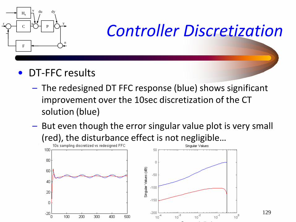
Controller Discretization
• DT-FFC results – The redesigned DT FFC response (blue) shows significant
improvement over the 10sec discretization of the CT solution (blue)
– But even though the error singular value plot is very small (red), the disturbance effect is not negligible…
P C
Hu
F
y u r
du dy v
n

130
Controller Discretization
• DT-FFC results – The explanation is that the DT solution is accurate (no
“unstable” zeros) but only for piecewise constant inputs in 10sec intervals. Our disturbance is a continuous sinusoid.
P C
Hu
F
y u r
du dy v
n
– Unfortunately real disturbances are not ZOH-sampled and lower sampling rates are detrimental to controller performance
– Indeed, when adding a ZOH after the disturbance source, the DT redesigned FFC works very well while the CT discretized does not.

131
Model Identification
• Parametric Model Identification from I/O data. – Non-parametric vs. Parametric models – Model parameterization: y = P[u;θ] – Estimation error (to be minimized) – Batch/Recursive update equations
• For more details: Notes on adaptive algorithms, http://www.eas.asu.edu/~tsakalis/notes/ad_alg.pdf
• other bibliography: Ljung, Soderstrom-Stoica, Ioannou-Sun, Goodwin-Sin

132
Model Identification
• Data conditioning (pre-processing): avoid estimation of uninteresting effects – High frequency filtering – Offset and Drift removal (low-frequency filtering)
• Justified by linearization principles – Scaling/conditioning
• Numerical Sensitivity, uncertainty interpretations • Speed of convergence in recursive algorithms
• SNR and record-length issues
133
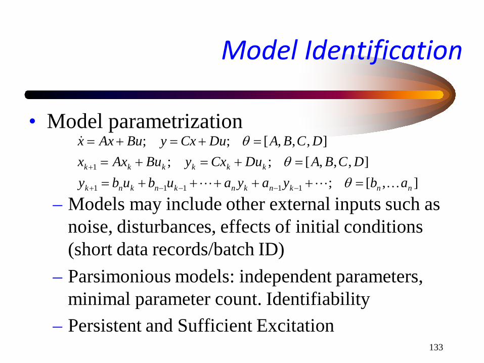
Model Identification
• Model parametrization
– Models may include other external inputs such as noise, disturbances, effects of initial conditions (short data records/batch ID)
– Parsimonious models: independent parameters, minimal parameter count. Identifiability
– Persistent and Sufficient Excitation
],[;],,,[;;
],,,[;;
11111
1
nnknknknknk
kkkkkk
abyayaububyDCBADuCxyBuAxx
DCBADuCxyBuAxx
=+++++==+=+=
=+=+=
−−−−+
+
θθ
θ

134
Model Identification
• Parameter Estimation Objective – Estimation error formulation, equation error – e = y - φTθ; φ = regressor.
• Linear-in-the-parameters (efficient algorithms exist) • Left factorization (observer), Coprime factor uncertainty
– e = y - P[u;θ] • Usually NonLinear-in-the-parameters • Additive uncertainty
– …
135
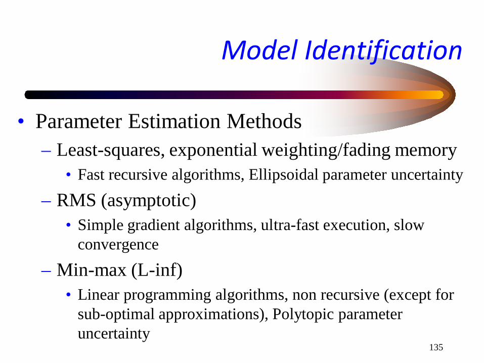
Model Identification
• Parameter Estimation Methods – Least-squares, exponential weighting/fading memory
• Fast recursive algorithms, Ellipsoidal parameter uncertainty – RMS (asymptotic)
• Simple gradient algorithms, ultra-fast execution, slow convergence
– Min-max (L-inf) • Linear programming algorithms, non recursive (except for
sub-optimal approximations), Polytopic parameter uncertainty

136
Model Identification
• Estimation algorithms – Linear model estimation error ek = yk - φk
Tθk
– λ: exponential weighting (forgetting factor). Typical values 0.990-0.999; depends on the number of parameters, excitation properties, parameter variations with time, etc.
10,1
:Squares-Least
0,1
:Gradient
11
1
1
≤<
+=
+−=
>+
+=
++
+
+
λ
φθθφφλ
φφλ
φφφθθ
kkkkk
kkT
k
kT
kkkkk
kT
k
kkkk
ePPPPPP
PPeP
137
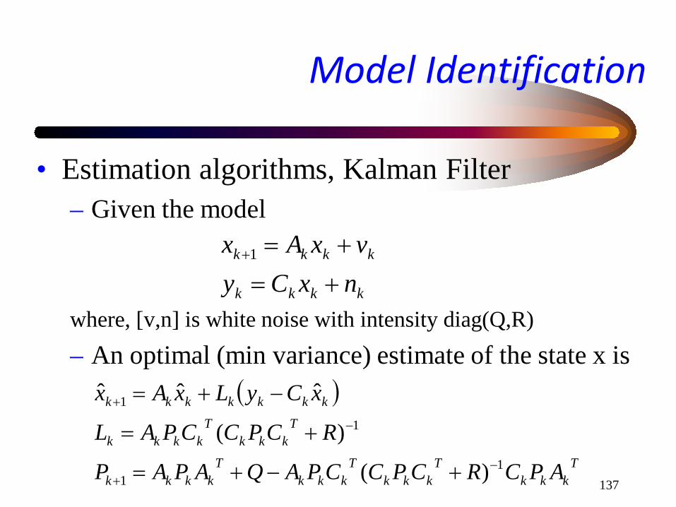
Model Identification
• Estimation algorithms, Kalman Filter – Given the model
where, [v,n] is white noise with intensity diag(Q,R) – An optimal (min variance) estimate of the state x is
kkkk
kkkk
nxCyvxAx
+=+=+1
( )
Tkkk
Tkkk
Tkkk
Tkkkk
Tkkk
Tkkkk
kkkkkkk
APCRCPCCPAQAPAP
RCPCCPAL
xCyLxAx
11
1
1
)(
)(
ˆˆˆ
−+
−
+
+−+=
+=
−+=

138
Model Identification
• Kalman Filter details – Assumptions: R>0, (A,C) observable, (A,Q) controllable – P-update: at steady-state becomes the discrete time filter
algebraic Riccati equation. Its positive definite solution guarantees that (A-LC) is stable.
– Returning to our estimation problem, write the linear model as a dynamical system
– and apply KF
( )k
Tkkk
Tkkkkk
kkT
kkkkkT
kkkkk
PRPPQPP
RPPLyL
φφφφ
φφφθφθθ1
1
11
)(
)(,ˆˆˆ−
+
−+
+−+=
+=−+=
kkT
kkkkk nyvI +=+=+ θφθθ ,1

139
Model Identification
• Take R=1 (for a scalar output) and Q --> 0 to recover the standard LS updates – Some expressions may “look” different but they become identical after
some algebraic manipulations
• Observability is equivalent to persistent excitation of φ • The difference in implementation becomes important when
adding constraints to parameters • The KF handles parameter variations naturally through the
noise term v and its covariance Q; if desired an exponentially weighted formulation can be derived to obtain the previous expressions; although it is not equivalent, the effect is similar

140
Model Identification
• An alternative algorithm for System Identification: Concatenate parameters and states into a big model (still linear but time-varying) and apply KF – this requires the system description in an observable form
(left factorization); its generality is justified as follows:
– F,C are design parameters: F should be stable and (F,C) should be observable
kkk
kkk
kkk
kkk
DuCxyuLDBLyFxBuLCxxLCA
BuAxx
+=−++=
++−=+=+
)()(
1
kkk
kkkk
uCxyuyFxx
3
211
θθθ
+=++=+⇒

141
Model Identification
• Collect states and apply KF to estimate both states and parameters
– Notice that the model is nonlinear in the states and parameters but it
becomes linear if the output is measured (and becomes an external time-varying parameter).
– Drawback: output additive noise enters nonlinearly in this model – Choose Q11 >>Q22 (states vary much faster than parameters) – Convergence condition is again the persistence of excitation
=
=
+
+
+
+
k
k
k
k
kk
k
k
k
kkk
k
k
k
k x
uCy
x
II
IIuIyFx
,3
,2
,1
,3
,2
,1
1,3
1,2
1,1
1
],0,0,[,
0000000000
θθθ
θθθ
θθθ

142
Model Identification
• Other Issues – Persistent excitation – Possible parameter drifts in the absence of
sufficient excitation (noise can mask the system) • Various modifications: Parameter projection, dead-zone,
regularization noise, excitation monitoring – Modeling and estimation of dynamic uncertainty
(region of model validity; analysis of residuals)
N allfor ,0:0, >>>∃ ∑+
=
InnN
Nk
Tkk δφφδ

143
Model Identification
• Estimator modifications – Parameter projection
• Knowledge of a convex set containing the parameters; find the best estimate in the set
– Dead-zone • Do not update when the error is below the noise level
– Regularization noise • Add artificial noise to the I/O pair used for estmation.
Penalizes large estimates (~ min norm solution), ensures covariance boundedness, at the expense of a small bias
– Excitation monitoring (high level logic)

144
Model Identification
• Example – Temperature control of a heating element with on-
line identification of its transfer function (Experiment 5)
– Plant (top layer)

145
Model Identification
• Example – Plant model
146
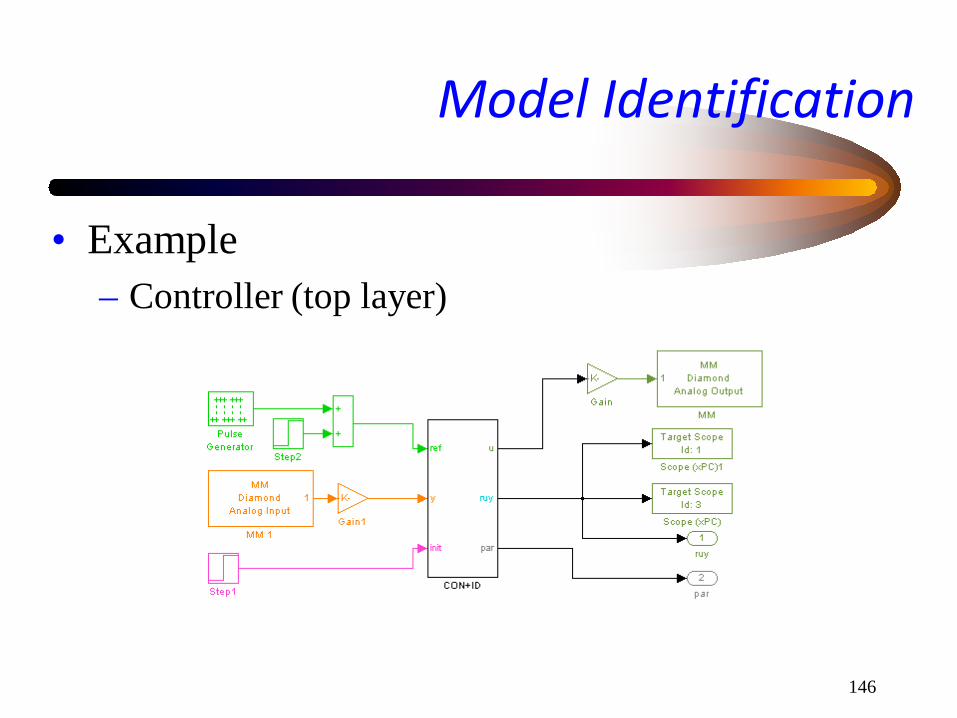
Model Identification
• Example – Controller (top layer)

147
Model Identification
• Example – Controller block: PID, LSE
148
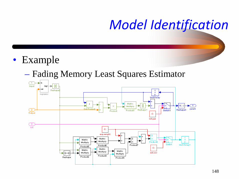
Model Identification
• Example – Fading Memory Least Squares Estimator

149
Model Identification
• Example – Experiment with different regularization noise levels,
different estimators • LS parameter (textbook), LS/KF parameter (notes), KF
parameter+state (notes) – Get familiar with the embedded function block and analyze
the impact on execution speed – Try different model orders, add disturbances and monitor
the excitation for different reference inputs… – Use prefilters on I/O data to remove nonlinear DC bias from
linearization

150
Model Identification
• Example – Supplied functions:
• Various estimator blocks (in idblocks) • Code to extract the state-space or transfer function
model from the parameter vector in comments inside each block; remember to adjust the code when changing the model order or model structure
• exp6KF.mdl contains a non-real-time version of the simulator to illustrate the operation of the parameter estimators

151
Instrument Ratings
• Usually static characteristics from manufacturers – Sensitivity: output magnitude to unit input – Dynamic range: upper-lower limits. Often
expressed as a ratio in dB, usually range/resolution
– Resolution: smallest change that can be detected – Linearity: maximum deviation from straight line – Zero/full scale drift: drift when input is
maintained steady for a long period

152
Accuracy-Precision
• Errors can be deterministic (systematic) or random – Measurement accuracy = closeness of the
measured value to the true value – Instrument accuracy = worst case accuracy within
the dynamic range – Precision = reproducibility or repeatability
• precision = measurement range/error variance • precision ~ measurement variance for constant input

153
Significance in measurement and computations
• Is a measurement 0.1V the same as 100mV? Or, is a resistance value 4.7kΩ = 4700Ω? What is the current flowing through a 3.3kΩ resistor when the voltage is 1.0V?
• Unless otherwise specified, the value is accurate to within 1 (or 1/2) least significant digit. So, – 0.1V = 0.1V +/- 0.1V – 100mV = 100mV +/- 1mV = 0.100V +/- 0.001V

154
Significance in measurement and computations
• In computations, the answer should have the same significant digits as the least of the numbers used in the calculation: – Current = Voltage / Resistance = (1.0 /3.3k)A =
(0.3030…m)A = 0.30mA – Significant digits: digits past first nonzero digit 1.0V/3300Ω = (0.0003030…)A = 0.00030A – Note: calculators compute with a fixed number of digits. Scientific
notation is consistent with the significant digit concept.
from computation
155
Sensors and Actuators
• Sensors: – “Process Variable” to “Data” conversion – Change in certain material properties with changes
in a process variable – Variety of sensor outputs: Electrical
(potentiometers, thermocouples, thermistors, strain gauge), mechanical (bi-metallic thermometers), numeric (counters, optical sensors)

156
Examples of Sensors and Actuators
• Actuators: – “Data” to “Process manipulated variable”
conversion – Variety of actuator inputs: Electrical (analog
control circuits), numeric (computer control systems), pneumatic (some industrial controls)
– Actuators/Final Control Elements: Heater (electric coil, gas burner, steam flow), Valve (pneumatic, solenoid, motor-driven), Light, Relay, Switch

157
Sensors
• Sensor Signal Conditioning – Convert signals to a form suitable for interfacing
with the other elements of the process control loop – Digital form: advantages in computations,
maintenance, reliability, cost – Typical operations: Amplification, Linearization,
Filtering and Impedance Matching

158
Sensors: Signal Conditioning
– Type of signal (variation/range) is usually fixed, depending on physical properties, (e.g., changes in resistance, voltage, etc).
– Amplification: Adjust the usually low signal level. Input impedance (transfer function) is important to assess speed of sensor response
– Linearization: Usually required; mild to severe nonlinearities; look-up tables and fitting functions; accuracy vs. precision

159
Sensors: Signal Conditioning
– Signal Conversion example: change in resistance to change in voltage or current
– Bridges to handle small fractional changes in resistance
– Analog Filtering to reduce aliasing effects. – Impedance matching to improve dynamics and
sensor signal strength (a power transfer problem) – Active or passive filters; input impedance
considerations

160
Sensors: Signal Conditioning
– Wheatstone bridge, current balance bridge: detection of a null condition (irrespective of voltage drifts)
∆V V
))(( 4231
4132
RRRRRRRRVV++
−=∆
Current balance bridge I s.t. ∆V = 0
R4>>R5 Ι
V ∆V

161
• Thermal Energy ~ atom vibrations, atom speed – Average energy per molecule – Different Scales (K,C and R,F) – Thermal Energy of one molecule
• 3/2 kT, k = 1.38 10-23 J/K (Boltzmann) – Average thermal speed
• O2, 90F, v = 488m/s
• Key sensor property: resistance vs Temperature
Thermal Sensors
mkT3
162
• Metal resistance increases with temperature (more electron collisions). – Resistance Temperature Detector (RTD) – Pt: almost linear in [-100,600], repeatable, 0.004/oC
sensitivity. – Ni: nonlinear, less repeatable, 0.005/oC sensitivity – measurement with a bridge – response: time for wire to acquire temperature – self heating effect from power supply (~1oC)
Thermal Sensors

163
• Semiconductor resistance decreases with temperature (more free electrons): Thermistors – highly nonlinear resistance variation with temp. – effective range [-100,300] oC – Insensitive at high temperatures – 0.5-10s response time (depending on sensor mass
and environment) – encapsulation material issues
Thermal Sensors
164
• Thermocouples: thermo-electric effect in a junction of different metals, voltage generation vs. temperature – Require cold junction reference – Almost linear; linearization tables for accuracy – Good range, sensitivity, inertness – Type J: [-200,700]oC, 0.05mV/oC, max 43mV – Type K: [-190,1260]oC, max 55mV – Type R: [0,1482]oC, 0.006mV/oC, max 15mV
Thermal Sensors

165
• Thermocouple signal conditioning – x100 amplification, susceptible to electrical noise
and E/M interference • twisted wires, grounded sheath, grounded junction • Reference compensation circuits with precision thermistors
• Bimetallic strips (volume expansion) • Gas thermometer (sensitive but slow)
– vapor pressure, liquid expansion, solid-state • Pyrometers (more details in optical sensor section)
Thermal Sensors

166
• Displacement-location-position – Ex. liquid level, object position/orientation, infer
pressure – Potentiometers: resistance and wiper
• wear, friction, resolution, noise; but linear and simple – Capacitance: C = Kε0A/d
• ex. movement of one plate changes area; measurement with an AC bridge
– Inductance: Armature moving through a coil
Position-Motion Sensors

167
• LVDT: Linear Variable Differential Transformer – Key component of many sensors – 2um resolution in commercially available systems
Position-Motion Sensors
moving core
primary coil
~ secondary
coil secondary
coil
Vout
- Difference in secondary coil voltages is linear with displacement. - Phase shift indicates direction of motion.

168
• Level sensors – Float with a secondary displacement measuring
system (e.g., LVDT) – Based on capacitance or conductivity properties of
the fluid – Ultrasonic non-contact sensor (measuring reflection
time) – Pressure-based sensor
Position-Motion Sensors

169
• Motion types – rectilinear motion (v,a), ~10g acceleration – angular motion (rotation) – vibration, ~100g, cos wt -> w2cos wt – shock (impact), ~500g
• Motion sensors – Accelerometers (mass-spring) – Natural frequency
Position-Motion Sensors
mkfN π2
1=

170
• f < fN/2.5: fN has little effect on response • f > 2.5 fN: response independent of applied frequency; a
vibration measurement; the “seismic mass” remains roughly stationary
– Potentiometric accelerometers: ~30g, steady-state acceleration, low frequency vibrations
– LVDT: 80Hz, Variable reluctance (LVDT-like), 100Hz, vibration only, geophones
– Piezoelectric: 2kHz, shock and vibration apps.
Position-Motion Sensors: accelerometers

171
• Pressure basics – F/A, units Pa, psi, Atm, bar. (1bar ~ 1atm ~ 100kPa
~ 14.7psi) – Static pressure (no flow). – Dynamic pressure (flow-dependent) – Gauge pressure (pabs - patm) – Head pressure (ρgh, static)
Pressure Sensors
172
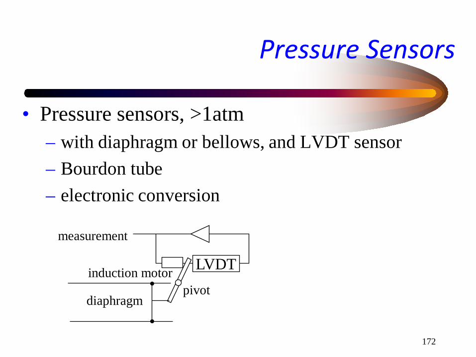
• Pressure sensors, >1atm – with diaphragm or bellows, and LVDT sensor – Bourdon tube – electronic conversion
Pressure Sensors
LVDT induction motor
diaphragm pivot
measurement

173
• Pressure sensors, <1atm (electronic) – Pirani gauge. Filament temperature via resistance
measurement or thermocouple-based; nonlinear pressure dependence); 10-3atm, calibrated for the type of gas.
– Ionization gauge 10-3- 10-13atm • heated filament - electrons - ionized gas - current between
electrodes • approximately linear
Pressure Sensors

174
• Stress = F/A; tensile, compressional, shear • Strain = ∆l/l; tensile, compressional, shear • Modulus of elasticity (Young) E = stress/strain
– linear for low stress, elastic region • Strain gauge: resistance change ~ strain
– order of 0.1% fractional change – temperature compensation necessary (temperature
effects are more significant)
Strain Sensors
175
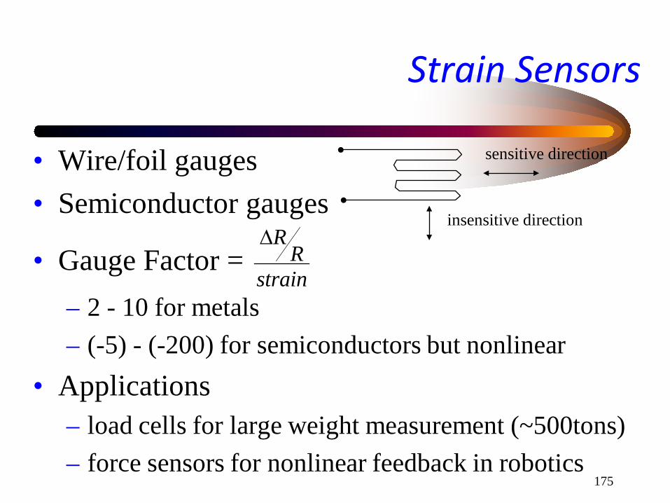
• Wire/foil gauges • Semiconductor gauges
• Gauge Factor = – 2 - 10 for metals – (-5) - (-200) for semiconductors but nonlinear
• Applications – load cells for large weight measurement (~500tons) – force sensors for nonlinear feedback in robotics
Strain Sensors
insensitive direction
sensitive direction
strainR
R∆

176
• Conveyor belt – load cell with strain gauge: measure weight on a fixed
length of belt; belt speed is given/measured • Liquid (volume or mass flow)
– restriction (Venturi, orifice plate, nozzle) – obstruction: rotameter (liquid/gas), moving vane
(angle~flow), turbine (tachometer~flow) – magnetic, (conductors/insulated pipe): flow through a
magnetic field and measure the transverse potential
Flow Sensors
pkQ ∆~

177
• EM radiation spectrum
Optical Sensors
Band Frequency Wavelengthc = λf
VLF MHz 300m
TV/radio MHz-GHz 0.3m
Microwave THz 0.3mm
Infrared 1015Hz 0.3um
Visible 400-760nm
UV 1017Hz 3nm

178
• Photo detectors – spectral response (wavelengths) – time-constant, response time – detectivity
• Photo conductive detectors – semiconductor conductivity (or resistance) as a
function of radiation intensity – resistance drops as number of absorbed photons with
higher energy than band gap increases
Optical Sensors
179
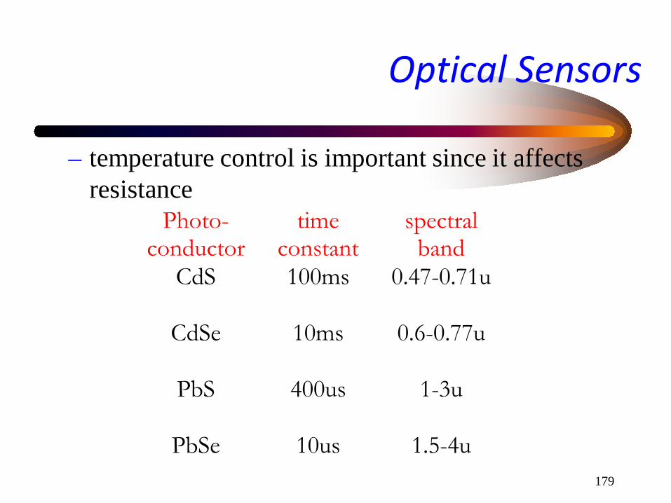
– temperature control is important since it affects resistance
Optical Sensors
Photo-conductor
timeconstant
spectralband
CdS 100ms 0.47-0.71u
CdSe 10ms 0.6-0.77u
PbS 400us 1-3u
PbSe 10us 1.5-4u

180
• Photo Voltaic detectors – “giant diodes”, V = Vo log(I) – time-constants: Si (20us), Se (2ms), Ge (50us), InAs
(1us) – photodiode detectors (changes in I-V characteristics):
1us - 1ns response time (for communication apps) – photoemissive detectors: current ~ light intensity,
photo-multipliers, very sensitive
Optical Sensors

181
• Pyrometers – Temperature ~ emitted EM radiation; black body
radiation ~ T4 (total) – Broadband pyrometers, total radiation pyrometers
• micro-thermocouple on blackened Pt disc; heats up with radiation and thermocouple generates a voltage; responds to all wavelengths
– IR pyrometer (Si-Ge)
Optical Sensors

182
• Pyrometer applications – Metal production, glass production, semiconductors – range 0-1000oC – accuracy 0.5-5oC – noninvasive – Correction factors – Contamination issues (viewport fogging)
Optical Sensors

183
• Optical light sources – conventional: incandescent, atomic (distributed,
divergent, incoherent, polychromatic) – Laser (monochromatic, coherent, non-divergent)
Optical Sensors
He-Ne red 0.5-100mW (cont) ranging alignment, comm.
Ar green 0.1-5W (cont) heat, small welding, comm.
CO2 IR 1-100kW (cont-pulse)
cutting, welding, drilling, comm.
Ruby red 1GW (pulse) cutting, welding, drilling, comm.

184
• Incremental Optical encoders – Identical, equally spaced transparent windows – Two photodiodes, quarter pitch apart (to establish direction). – Angle of rotation is the summation of pulse counts (rising
edge). – Velocity is window spacing by elapsed time. – Resolution is: N = windows, T =
sampling time – e.g., 10,000 windows => 0.018o resolution
Optical Sensors
NTNπωπθ 2,2
=∆=∆

185
• Absolute Optical encoders – Code pattern on the encoder disk – N tracks to provide 2N resolution (N ~ 14), each track
associated with a pick-off sensor – Gray coding: one bit switching between adjacent sectors;
minimizes errors due to manufacturing tolerances (e.g., eccentricity)
Optical Sensors

186
Actuators and Final Control Elements
• Implementing changes in process variables – Relays, SCR/TRIAC (motor and heater control) – Amplifiers (Analog, PWM) – Solenoids (electromechanical conversion)
• coil and plunger; free standing or spring loaded
– Motors • DC: series field (hi-torque, difficult speed control);
shunt (lower torque, easy speed control); compound • AC (Synchronous-Asynchronous, Low starting torque) • Stepping

187
Actuators and Final Control Elements
– Pneumatic signals: pressure as information carrier • 3-15psi standard , 330m/s propagation (sound)
– Amplifiers (diaphragm-based), Hydraulics • Nozzle-Flapper (mechanical-pneumatic conversion) • Diaphragm-Spring (pneumatic-mechanical conversion) • Current-2-Pressure conversion (solenoid-nozzle-flapper)
– Valves (Quick open, Linear, Equal Percentage) – Hopper valves (solids), Rollers

188
Actuators
• Push-pull class B amplifier. (Use multiple stages, if necessary)
• Pulse Width Modulated (PWM) amplifiers – Varying the duty cycle of a square wave – Efficient switching transistors for high power
requirements
DAC
V+
V-
Complementary pair of transistors

189
Actuators
• Silicon-Controlled Rectifier (SCR, thyristor) – trigger voltage at the gate will start conducting
positive voltages from anode to cathode; it will stop when the forward bias at the gate is off and the anode voltage is negative (half-wave operation)
– TRIAC: full-wave operation – Power Control for high power applications (e.g.,
heating) SCR
half-wave operation
Vload
Vgate

190
Bibliography
• Curtis Johnson, Process Control Instrumentation Technology, 4th ed. Prentice Hall, New Jersey 1993.
• Lennart Ljung, System Identification: Theory for the User. Prentice Hall,