eeee',e - defense technical information center · sor routine called pilestf that can compute...

A-AOA7 191 ARMY ENGINEER WATERWAYS EXPERIMENT STATION VICKSBURG MS F/6 13/13

DOCUMENTATION FOR LMVDPILE PROGRAM. (U)JUN 80 D K MARTIN, H A JONES, N RADHAKRISHNAN

UNCLASSIFIED WES TR K 80 -3L

EEEE',E

_LEVETEC4NICAL REPORT K-80-3

DOCUMENTATION FOR LMVDPILEPROGRAM

by

Deborah K Martin, 14. Wayne Jones, N. Radhakrishn

lI>. Automatic Data Processing CenterU. S. Army Engineer Waterways Experiment Stii

P. 0. Box 631, Vcksburg, Miss. 39180

IJue 1980Final Report S

o A~~,pprove Far rubk Ref"es. ODtwbutio UalhNltd

-5 Prmped for U. S. Army Engineer Dision, Lower Mississippi Valley- P. 0. Box 80, Vicksburg, Mls. 39180

*~' C.. tRMIS D0C' flNT IS BEST QUALITY RATIUWAI sIU TO COPM U R IWNIS' TO DDC CONTAINID LA

SIGNIFICANT NUMBER OF Fk MZ WHOH DIRM,0DUCE LEGIBLY% 0

~iM80 7 28098

Destroy this report when no longer needed. Do not returnit to the originator.

The findings in this report ore not to be construed as an officialDepartment of the Army position unless so designated

by other authorized documents.

DISCLAIMER NOTICE

THIS DOCUMENT IS BEST QUALITYPRACTICABLE. THE COPY FURNISHEDTO DTIC CONTAINED A SIGNIFICANTNUMBER OF PAGES WHICH DO NOTREPRODUCE LEGIBLY.

UnclassifiedSECURITY CLASSIFICATION OF THIS PAGE (When Date Entered_

REPOT DCU HT TOH AGEREAD INSTRUCTIXONSREPORT DOCUMENTATION PAGE BEFORE COMPLETING FORM

1. REPORT NUMBER / 2. GOVT ACCESSION NO. 3. RECIPIENT'S CATALOG NUMBER

Techinical Report i(-80-3 714. TITLE (and Subtitle) S. TYPE OF REPORT A PERIOD COVERED

DOCUMENTATION FOR LMVDPILE PROGRAMp Final /I / 4.- " _--.'c '-': z ' 004. W 14:.i_"UMBERS

/

7. AUTHOR(s) B. CONTRACT OR GRANT NUMBER(&)

Deboah Martin N. adhrishnanH. Wayne/Jones /R.... .......

.PERFORMING ORGANIZATION NAME AND ADDRESS10 RA PtErU. S. Army Engineer Waterways Experiment Stationv AREA & WORK UNIT NUMBERS

Automatic Data Processing Center ) .7P. 0. Box 631, Vicksburg, Miss. 39180

II. CONTROLLING OFFICE NAME AND ADDRESS 12. REPORT DATE

U. S. Army Engineer Division, June 180Lower Mississippi Valley 13. NUMBER OF PAGES

P. 0. Box 80, Vicksburg, Miss. 39180 18814. MONITORING AGENCY NAME & ADDRESS(If different from Controllind Office) IS. SECURITY CLASS. (of this report)

- . ,Unclassified

1 - IS&. DECLASSI FICATION/DOWNGRADINGSCHEDULE

IS. DISTRIBUTION STATEMENT (of this Report)

Approved for public release; distribution unlimited.

17. DISTRIBUTION STATEMENT (of the abstract entered In Block 20, If different from Report)

If. SUPPLEMENTARY NOTES

IS. KEY WORDS (Continue on reveree side if necessary mid identIfy by block number)

Computer programs LMVDPILE (Computer program)

Computerized simulation Pile capsDocumentation Pile foundationsMatrix analysis

111. ),"ACT mf l, mi . i n--my mi Identf by block manmbe)The primary work reported here consists of consolidating the rigid cap pile

analysis programs of the U. S. Army Engineer Districts, St. Louis and NewOrleans. The new program, LMVDPILE, is documented with example problems in thisreport. The work was performe- at the request of the Lower Mississippi ValleyDivision and provides the capability of analyzing two-dimensional or three-dimensional pile foundations according to Division guidelines. The report in-cludes discussions of factors influencing pile group behavior and of the

(Continued)

D M m-o, or i Iov so is OOoLETE Unclassified

SECUMTV CLASSIFICATION OF THIS PAGE (WMen Deta Entersd)

UnclassifiedSECURITY CLASSIFICATION OF THIS PAGE(3k., Data BateE)

20. ABSTRACT (Continued).

analytical procedure, a user's guide, and several example problems for the pileanalysis program LMVDPILE. Also included are two appendices. Appendix A des-cribes the computer program PILESTF which computes the pile head stiffness coef-ficients for piles in soils with varying moduli. Appendix B describes the com-puter program FDRAW which is an interactive graphics post-processor. Eachappendix includes a general introduction, a user's guide, and example problems.

/

Accession For /

NTIS GRO.,&I

DDC TAB

UnannounlcedJust if ic. t ion ....

Dist' r cut al

Unclassified

SECURITY CLASSIFICATION OF THIS PAGE(IP9ff Data Ent-ee)

PREFACE

The study reported herein was performed at the U. S. Army Engineer

Waterways Experiment Station (WES) as part of the support provided by

the Computer-Aided Design Group (CADG) of the Automatic Data Processing

(ADP) Center to the U. S. Army Engineer Division, Lower Mississippi

Valley (LMVD).

The work involved consolidation of two existing pile analysis pro-

grams, one from the St. Louis District and the other from the New

Orleans District. This work was performed by Ms. Deborah K. Martin,

formerly of CADG. The computer program PILESTF which is described in

Appendix A was coded and documented by Dr. William P. Dawkins, Consul-

tant, Oklahoma State University, Stillwater, Okla. PILESTF computes the

pile head stiffness coefficients for piles in soils with varying moduli.

The computer program FDRAW which is described in Appendix B was coded

and documented by Mr. John Jobst of the St. Louis District. FDRAW is an

interactive graphics post-processor program that can display pile geome-

try, resultant axial forces, pile loading factors, and elastic center

diagrams. The authors thank Dr. Dawkins and Mr. Jobst for their contri-

butions to this work.

This report was written by Ms. Martin, Mr. H. Wayne Jones, CADG,

and Dr. N. Radhakrishnan, Special Technical Assistant, ADP Center.

Technical contact at the St. Louis District was Mr. Thomas J. Mudd and

at the New Orleans District was Mr. C. W. Ruckstuhl. The authors thank

Mr. Mudd, Mr. Ruckstuhl, and several of their co-workers for their

technical guidance.

The study was monitored at LMVD by Mr. Victor Agostinelli, Techni-

cal Engineering Branch. The work was done under the general supervision

of Mr. D. L. Neumann, Chief of the ADP Center.

COL J. L. Cannon, CE, and COL N. P. Conover, CE, were Directors

and Mr. F. R. Brown was Technical Director of WES during the performance

of the work and the preparation of the report.

CONTENTS

Page

PREFACE .............. ............................. 1

CONVERSION FACTORS, U. S. CUSTOMARY TO METRIC (SI)UNITS OF MEASUREMENT ....... ..................... . .. 4

PART I: INTRODUCTION ........... ...................... 5

Background .......... . ......... ................ 5Scope ............. ........................... 5

PART II: FACTORS INFLUENCING PILE GROUP BEHAVIOR .... ........ 6

Factors that Influence Capacity of Pile Foundations .... 6Conclusion ............ ......................... 9

PART III: PROCEDURE FOR THE ANALYSIS OF PILE FOUNDATIONS . . . . 10

The General Model .......... ..................... 10Analysis .......... .......................... . l.11Failure Criteria ........... ...................... 25

PART IV: USER'S GUIDE FOR PROGRAM LMVDPILE ... ........... ... 28

General Introduction ........ .................... ... 28Flow Charts ............ ........................ 29Data Input for LMVDPILE ...... .................. ... 29

PART V: EXAMPLE PROBLEMS ........ .................... ... 41

Example Problem 1 - Two-dimensional problem, 2 pinnedpiles with constant soil modulus .... ............. ... 41

Example Problem 2 - Two-dimensional problem,1 fixed vertical pile ...... .................. ... 53

Example Problem 3 - Two-dimensional problem,Hrennikoff's example case 2a ..... ............... ... 58

Example Problem 4 - Two-dimensional problem,Hrennikoff's example case ha ..... .............. ... 63

Example Problem 5 - Two-dimensional problem,Hrennikoff's example case 6a .... ............... 68

Example Problem 6 - Two-dimensional problem, 16 pileswith linearly varying soil moduli ... ............ ... 73

Example Problem 7 - Three-dimensional problem, 4 pinnedpiles and constant soil modulus .... ............. ... 83

Example Problem 8 - Three-dimensional problem,1 fixed vertical pile ...... .................. ... 96

Example Problem 9 - Three-dimensional problem, 27 pileswith constant soil modulus ........ ................ 101

Example Problem 10 - Three-dimensional problem, 9 pilesand linearly varying soil moduli ..... ............. l0

Example Problem 11 - Three-dimensional problem, 60 pileswith linearly varying soil moduli ...... ............ 117

REFERENCES ........... ........................... ... 132

2

Page

APPENDIX A: USER'S GUIFE FOR PROGRAM PILESTF .. .......... Al

General Introduction. .. ................... AlBackground. .. ........................ AlPrevious Pile Head Stiffness Evaluation. ........... A3Alternate Derivation .. ................. ... A7General Pile Head Stiffness Analysis Introduction .. .... A10Pile-Soil Model. .................. .... A10Soil Springs .. ................... .... AllElement Force-Displacement Relations. ... ......... A12Nodal Equilibrium. ................. .... A13Special Conditions at Node m (Bottom of Pile) ... ...... Al4Special Conditions at Node o (Pile Head). ..... ..... Al4Guide to Data Input ... ................... A18Example Solutions .... ................... A19Discussion of Results .... ................. A21Conclusions. .................. ...... A21

APPENDIX B: USER'S GUIDE FOR PROGRAM FDRAW .. ........... B1

General Introduction .. ................ .... BlGuide for Data Input .. ..................... B3Example Problems .. .................. .... B5

3

CONVERSION FACTORS, U. S. CUSTOMARY TO METRIC (SI)UNITS OF MEASUREMENT

U. S. customary units of measurement used in this report can be con-

verted to metric (SI) units as follows:

Multiply By To Obtain

feet 0.3048 metres

inches 2.54 centimetres

kips (1000 lb 4.448222 kilonewtonsforce)

kips (force) per 47.88026 kilopascalssquare foot

pounds (mass) 0.45359237 kilograms

pounds (force) per 6.894757 kilopascalssquare inch

pounds (mass) per 16.01846 kilograms per cubiccubic foot metre

pounds (mass) per 0.02768 kilograms per cubiccubic inch centimetre

square inches 6.4516 square centimetres

-4

DOCUMENTATION FOR LMVDPILE PROGRAM

PART I: INTRODUCTION

Background

1. Many Corps of Engineers offices use the Hrennikoff (1950)

method to analyze pile foundations. This method was originally proposed

for analyzing two-dimensional pile foundations but has been refined and

extended by Saul (1968) for three-dimensional foundations.

2. The U. S. Army Engineer Districts, St. Louis and New Orleans,

each use a different version of a pile analysis computer program, but

both use the Hrennikoff method. The Technical Engineering Branch of

the Lower Mississippi Valley Division (LMVD) was interested in standard-

izing the two Districts' programs into one program, LMVDPILE, that would

include all options from both programs. The work described herein was

performed at the request of LMVD. The result of this work provides the

capability of analyzing two-dimensional or three-dimensional pile founda-

tions according to the LHVD guidelines.

Scope

3. Factors influencing pile group behavior, the analytical proce-

dure, a user's guide, and several example problems for the pile analysis

program LMVDPILE are presented herein. User's guides for a pre-proces-

sor routine called PILESTF that can compute the pile head stiffness

matrix for a pile in a layered soil mass and for an interactive graphics

post-processor program, FDRAW, are also included.

5" UI

PART II: FACTORS INFLUENCING PILE GROUP BEHAVIOR*

4. Foundation piles are supporting str,ctural members which trans-

fer loads from the structure to the subsoil. Adequate design will insure

that excessive deflections and stresses in the "structure-pile-soil

system" will not occur. Generally, it is not a difficult task to deter-

mine the loads acting on the pile foundation from tife structure. How-

ever, the distribution of the loads from the piles to the soil is

highly indeterminate and sometimes nonlinear problem. This leads to

complex solutions of the pile-soil interaction problem. Many conditions

affect the resistance of the pile foundation to movement and the transfer

of loads from the structure to the pile-soil medium (Mudd 1969).

Factors that Influence Capacity of Pile Foundations

5. The capacity of a pile foundation can be defined as its ability

to resist applied loads without exceeding certain allowable deflections

or stresses. The following variables should be considered during analy-

sis of the load-carrying capacity of the soil-pile medium.

Subgrade modulus

6. A subgrade modulus can be employed to relate the lateral, axial,

and rotational resistance of the pile-soil medium to displacements. The

subgrade modulus is a function of the nature of the loading, the elastic-

ity of the pile, and the stress-strain characteristics of the surrounding

soil. Therefore, the determination of the subgrade modulus depends on

the nonlinear and nonelastic, pile-soil stress-strain relationshir char-

acteristics. The load-carrying capacity of the foundation is dependent

on these nonlinear and nonelastic characteristics.

Fixity

7. The fixity of the pile head into the pile cap influences the

load-carrying capacity of a pile foundation. Generally, fixing the pile

heads completely rather than pinning them into the pile cap will double

* MaJor portions of Part II are extracted from Mudd (1969).

6

the lateral stiffness of the foundation. Thus the fixed pile can carry

twice the lateral load with the equivalent deflection as the pinned

pile foundation.

Batter

8. The direction and slope of batter affect the subgrade modulus.

Murthy (1964) has shown with model pile tests that piles battered up-

stream are more resistant to lateral loads than piles battered down-

stream. A pile battered upstream is defined as having its tip further

upstream than its top, and a pile battered downstream as having its tip

further downstream than its top.

Group effect

9. Close spacing of piles will affect the lateral and vertical

resistance of adjacent piles within a pile group. Prakash (1962) has

shown that piles spaced from three to eight pile diameters apart (normal

to the load) cause a reduction in the lateral capacity of the group. A

pile spacing of less than three diameters decreases the stiffness of the

pile group by about one half of the sun of the same number of isolated

piles. The group effect can be accounted for by reducing the subgrade

modulus by an appropriate factor. Similar effects have been noted for

the axial capacity of group friction piles.

Position in group

10. Prakash has also shown that the position of the pile in a

group affects its individual stiffness influence coefficients. He has

shown that a pile in the interior of the group would be more flexible

than one on the perimeter. This is due to the interference of the zone

of influence of the pile by adjacent piles when these zones overlap.

Stiffness of pile cap

11. The stiffness of the pile cap will influence the distribution

of the structural loads to the individual piles. A multicolunn bent

can be approximated as having a rigid top if the cap is 10 or more times

stiffer than the columns. Therefore a rigid pile cap can generally be

assumed for gravity-type hydraulic structures. If the cap is less than

rigid, then the problem becomes one of achieving compatibility between

pile-head displacements and the structure deformation. The program

7

SAPIV has been modified to include a pile element (Jones and

Radhakrishnan 1975). This will allow the analysis of flexible pile

caps if necessary.

Nature of loading

12. The different conditions of static, cyclic, dynamic, and

transient loadings affect the ability of the pile foundation to resist

applied forces.

13. Cyclic loading (repeated application of a static load) causes

a greater deflection than the application of a sustained static load of

the same magnitude. In some pile tests the application of cyclic load-

ing doubles the deflection over that of the application of a single

static load for a given level of loading (U. S. Army Engineer District,

Little Rock 1964).

lh. Piles subjected to vibratory loads may produce greater pile

displacements than piles subjected to static loads. At present, little

is known of the quantitative effect vibrations may have on the load-

carrying capacity oi pile-founded structures.

15. If tension and compression piles are present in a foundation,

the tension pile may have a reduced load-carrying capacity from that of

the compression pile for equivalent deflections. Also, the tension pile

may have less lateral stiffness than an equivalent compression pile.

Pile driving

16. Driving piles in a group increases the density of the soil

within and around a pile group. Consequently the stiffness of the soil

may increase by driving piles in closely spaced groups. Although tests

on a single pile within a group may indicate an increased stiffness due

to pile driving, the pile group as a whole may not reflect this increased

stiffness. A larger zone of stressed soil may not be favorably affected

by pile driving. Thus deflections larger than anticipated may result.

Therefore, lateral load tests on a single pile in a large group of piles

may indicate liberal stiffness coefficients.

Water table and seepage pressures

17. The position of the water table affects the lateral subgrade

modulus. Effects of submergence have been accounted for by some

8

designers by reducing the lateral subgrade modulus by the ratio of sub-

merged unit weight of the soil to its dry unit weight. An additional

load on the pile foundation can be caused by seepage pressures under

structures that support unbalanced water loads. These seepage pressures

also may affect the subgrade modulus of the soil.

Sheet pile cutoffs

18. Sheet pile cutoffs inclosing the pile group may change the

distribution of stress in the soil, affecting the load-carrying capacity

of the foundation.

Length of pile

19. The length of a pile will affect the lateral and axial sub-

grade modulus. The lateral subgrade modulus is different for short

rigid piles that act as poles and long flexible piles that act in flex-

ural bending. Piles can be considered to act in the flexural mode if

the nondimensional length L/T is greater than 5, as defined by Reese

and Matlock (1960).

Conclusion

20. All these factors must be considered if a valid analysis of

pile foundations is to be accomplished. The effects of most of these

variables can be accounted for in the analysis by appropriate changes in

the value of the subgrade modulus obtained from pile test data of a

single free pile.

9

PART III: PROCEDURE FOR THE ANALYSTS OF PILE FOUNDATIONS*

21. A general direct stiffness analysis method for three-

dimensional pile foundations has been presented by Saul (1968), which

expands the Erennikoff (1950) method from two dimensions to three.

This method appears to be general, provided the designer has an under-

standing of matrix methods and structure-soil-pile interactions and an

electronic computer available to perform the computations. The method

uses exact numerical analysis solutions for solving the assumed soil-

pile model. However, the designer must have an adequate representation

of soil-pile interaction for input to the method. Various factors that

influence the soil-pile interaction have been discussed in Part II.

The General Model

22. A generalized model of the structure-pile system can be de-

scribed as a rigid body supported by sets of springs which represent

the actions of the pile forces on the structure when the structure

undergoes unit displacements. It is assumed that the pile head loading

for any single pile in a batter group may be resolved into a combina-

tion of axial load, bending moment, shear, and torque. Also, each of

these components can be represented by a proper spring constant and

results added vectorially to obtain the total movement of the pile

head. This method of analysis only considers the effect the piles

have on the pile cap at the top of the pile; i.e., each pile can be

replaced by the proper elastic spring restraints at the pile cap. The

assumptions required by this method are:

a. A rigid piling cap.

b. Elastic behavior of the system.

c. Effects of displacement for six degrees of freedom in athree-dimensional analysis or for three degrees of free-dom in a two-dimensional analysis can be superimposed.

*Major portions of Part III are extracted from Mudd (1969).

10

23. This method can also account for:

a. Any degree of fixity of any pile with the pile cap.

b. Piles with different bending stiffness about their princi-

pal axes.

c. Any degree of linear (elastic) torsional, axial, or lat-

eral resistance of any pile in the foundation.

d. Any position and batter of piles in the foundation.

e. Piles of different sizes or materials in the foundation.

2h. If the restrictions as stated in paragraph 22 are not allowed,

then the response of the system is nonlinear, and a closed form solu-

tion cannot be achieved. However, it is possible to include these in

some type of iterative procedure.

Analysis

Elastic pile constants,

three-dimensional system

25. Each pile has six degrees of freedom in a three-dimensional

system: two lateral, one axial, two moment, and one torsional. The

forces and displacements along the pile axes are shown in Figure 1 in

which axes U1 and U2 are principal axes of inertia and axis U3 coincides

with the longitudinal axis of the piling. In a two-dimensional system,

each pile has three degrees of freedom: one lateral, one axial, and

one moment. Figure 2 shows the forces and displacements along the pile

axes. The pile forces can be equated to the pile displacements by the

expression

(Fl. = {b}. (Xl. (1)1 1 2.

such that b. are the individual pile stiffness influence coefficients

called the elastic pile constants. The {b1 i matrix for a three-

dimensional system can be defined for the i pile as

F6 X6X

/ "~~~1 U I F = 3 X

FF 1 +5X3

F F4 X4

U2 5 X2

F2U3

PILE AND FORCES

STRUCTURE AXES (PILE OR STRUCTURE AXIS) DISPLACEMENTS

Figure 1. Coordinate system for three-dimensional system

F5

F3 X310w F1 s X1

PILE AND FORCES (PILE ORSTRUCTURE AXES STRUCTURE AXIS) DISPLACEMENTS

Figure 2. Coordinate syster for two-dimensional system

b 1 0 0 0 bl5 0

0 b22 0 b24 0 0

0 0 b33 0 0 0{bl, = (2)0 b42 0 b44 0 0

b 0 0 0 b 051 55

0 0 0 0 0 b6 6 .)

26. The elastic pile constants are defined as follows:b 1 is the force required to displace the pile head a unit

distance along the U -axis, FORCE/LENGTH

b is the force required to displace the pile head a unitdistance along the U 2-axis, FORCE/LENGTH

12

12

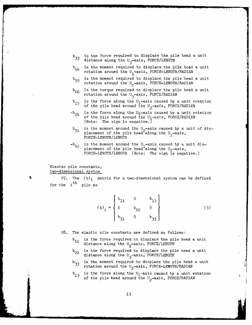
b33 is the force required to displace the pile head a unitdistance along the U 3-axis, FORCE/LENGTH

b44 is the moment required to displace the pile head a unitrotation around the U -axis, FORCE-LENGTH/RADIAN

b55 is the moment required to displace the pile head a unitrotation around the U 2-axis, FORCE-LENGTH/RADIAN

b66 is the torque required to displace the pile head a unitrotation around the U3-axis, FORCE/RADIAN

b15 is the force along the Ul-axis caused by a unit rotationof the pile head around the U 2-axis, FORCE/RADIAN

-b24 is the force along the U2-axis caused by a unit rotationof the pile head around the Ul-axis, FORCE/RADIAN

(Note: The sign is negative.)

b51 is the moment around the U -axis caused by a unit of dis-

placement of the pile head along the U -axis,FORCE-LENGTH/LENGTH

-b is the moment around the U -axis caused by a unit dis-placement of the pile head along the U2 -axis,FORCE-LENGTH/LENGTH (Note: The sign is negative.)

Elastic pile constants,two-dimensional system

27. The {bli matrix for a two-dimensional system can be definedth

for the i pile as

b l 0 b 1

fb}i= 0 b22 0 (3)b31 0 b33

28. The elastic pile constants are defined as follows:b 1is the force required to displace the pile head a unit11 distance along the U -axis, FORCE/LENGTH

b22 is the force required to displace the pile head a unitdistance along the U -axis, FORCE/LENGTH

3b is the moment required to displace the pile head a unit

rotation around the U 2-axis, FORCE-LENGTH/RADIAN

b13 is the force along the Ul-axis caused by a unit rotationof the pile head around the U 2-axis, FORCE/RADIAN

13

b 3 is the moment around the U -axis caused by a unit dis-placement of the pile head along the U -axis,FORCE-LENGTH/LENGTH 1

29. The elements for the {b}. matrix are symmetric. That is:

b15 b 51

b24 =b42

for a three-dimensional system. For a two-dimensional system,

b13 b31

Constant soil modulus

30. If it is assumed that the lateral subgrade modulus is con-stant with depth, then the pile constants for a three-dimensional system

can be derived as follows. If

J31 TI J 2 ' 32 r _ -4I,

then (E )bl1 = (.l + DF) 2-(5)

b22 = (1 + D) (6)

b33 = K2 (A) (7)

b = DF (8)

24 2 3)

14 '

j .3.-

b55 DF (9)

b6 6 = K 4 (10)

b DF (11)152

b24 =DF (12)242

b b15 (13)

b42 b24 (14)

where

E = lateral subgrade modulus, FORCE/LENGTH2*

E = modulus of elasticity, FORCE/LENGTH2

I,2 = moment of inertia, LENGTH 4 , about the U1and U2 axes, respectively

DF = degree of fixity (fraction)

Constants K2 and K 4 = degrees of pile rigidity under axial andtorsional behavior, respectively. K is

.2normally assumed to be 1.0 for bearingpiles and 2.0 for friction piles. K 4 isnormally assumed to be zero as the tor-sional behavior of the pile is not wellknown.

The lateral subgrade modulus Es required in the program input

should include width effect of the pile, group effect, cyclic loadeffect, etc. There are no provisions in the program to internallycalculate these effects.

15

A = cross-sectional area of pile, LENGTH2

L = length of pile, LENGTH

31. For a two-dimensional system, if

a1 =r (15)VE2

then

(_,Es1 = (1+DF) al (16)

b2 2 K2 ( ) (17)

b33 e3DF (18)

b13 DF (19)

b =b (20)31 13

Linearly varying subgrade moduli

32. If it is assumed that the lateral subgrade modulus varies

linearly with depth, Es = Ks(x3) then the pile constants for a three-s s3

dimensional system can be derived as follows. If

16

E12 _ 1 (21)T1 K s T2KS S

then

b =K -(22)11 1T3

22 K1 (23

b 3 3 K K2 (AL) (24)

bh k, I3 (25)

b K3 (E 2 ) (26)

b6 K K G) (27)

b1 K K5 (-9- (28)

17

- ~ ~ ~ ~ ~ ~ ~ 101 RIJE.~i OWN aR low~JJI~ IL

b 1( (I) (29)

b K6(? (30)

511

b 2 -K 6Q) (31)

where

E = modulus of elasticity, FORCE/LENGTH2

14IiI2 = moments of inertia, LENGTH , about U and U axes,

respectively 1 2

K = coefficient of subgrade modulus, FORCE/LENGTH3

A = cross-sectional area of pile, LENGTH2

L = length of pile, LENGTH

J = polar moment of inertia, LENGTH4

G = torsion modulus, FORCE/LENGTH2

K1 = lateral fixity coefficient

K2 = pile axial resistance coefficient

K3 = rota ional fixity coefficient

K4 = coefficient for torsion

K5 = fixity coefficient

K6 = fixity coefficient

33. For a two-dimensional system, if

T= (32)Ks

18 :

, , _i ... ...... ... .. . *1

then

b 1 E (33)

b2 K(LE (3)4)

b33 K 3 (~I) (

b13 K 5 () (36)

b3 1 K (37)

Fixity coefficients

34. The constants K1 through K6 depend on such variables as

the pile head fixity and the distribution of load from the pile to the

soil axially and torsionally. Values of K1 through K6 can be

derived for various degrees of fixity.

35. Knowing the degree of fixity, the following values of KI

through K6 can be derived for a lateral subgrade modulus that varieslinearly with depth:

19

Fixity Coefficients for Linear Subgrade ModulusDegree ofK K K KFixity (DF) 1 2 3 K4 5 6

1.0 1.0756 1.0 for bear- 1.4988 Torsion (as- 0.9990 0.9990

0.9 0.9263 ing or 2.0 1.3489 sumed 0.0 0.8991 0.7736for fric- by some

0.8 0.8129 tion piles 1.1990 designers) 0.7992 0.60350.7 0.7242 in compres- 1.0491 0.6993 0.4704

sion. For0.6 0.6530 piles in 0.8993 0.5994 0.3636

0.5 0.59145 tension 0.7494 0.4995 0.2759the value

0.4 0.5457 should be 0.5995 0.3996 0.2025

0.3 0.5042 reduced. 0.4496 0.2997 0.1404Suggest 1/2

0.2 o.4687 of value 0.2998 0.1998 0.0870

0.1 0.4378 for com- 0.1499 0.0999 0.0406pression

0.0 0.4107 piles. 0.0 0.0 0.0

36. The value of DF , degree of fixity of a pile into the cap

(expressed as a fraction), must be selected with a full understanding

of the conditions that must be met for a pile, which is assumed to be

fixed, to actually be fixed.

37. The fixity of the pile, DF , depends to a great extent on

the pile's embedment into the pile cap. A pretensioned prestressed

concrete pile is not fully fixed unless the extension of the pile con-

crete into the cap is at least as long as the bond development length

of the prestressing strands. Further, the pile cannot develop the full

moment capacity at the bottom of the cap. Any strand extension distance

beyond the end of the pile does not contribute to the bond development

distance because the strand elongation needed to develop the strand

prestress will cause excessive cracking and loss of rigidity of the

concrete. However, a posttensioned concrete pile can be considered

fully fixed with less embedment than a pretensioned pile if the tendon(s)

are tensioned to the cap after the cap is placed. A nonprestressed

concrete pile may be considered fully fixed by a bar extension equal to

the bond development length.

20

Orientation of thepile to the foundation

38. In a three-dimensional system the pile may be located at a

position rotated to the foundation axis and may be battered. Its posi-

tion in the pile cap is fully defined by the clockwise angle a. to1

the direction of batter and the batter slope hi , as shown in Figure 3.

The major principal axis of a pile i , where I I 12 should coincide

with the antle a. . The components of force and displacement of the

rotated pile axis to the foundation axis are found by the transformation

matrix {a). for pile i where1

h. = batter (h. Vertical on 1 Horizontal)1 1

a. = clockwise angle to the batter and/or major principal axis1

yi = arc cot h.

In a three-dimensional system

(cosy cosa) -sina (siny cosa)

{a'}i =(cosy sina) cosa (siny sina) (38)

-siny 0 cosy

U1

PARALLEL TOSTRUCTURE AXIS

01. ROTATION ANGLE 7I~ATE LP

LOCAL PILE AXIS(DIRECTION OF BA TTER)

U' U3

2 3,

PLAN SECTION A-A

Figure 3. Orientation of local pile axis andglobal foundation axis

21

and

f a). (39)0 a'

In a two-dimensional system

(cosy cosa) (siny cosa) 0fa}. = -siny cosy4 (h0)

0 0 Cosa

39. By the use of the transformation matrix the pile forces can

be rotated into forces parallel to the foundation axis by

{F'}. = {a). (F). (41)

1 1 1

and

{x}i {a). x'}i (42)

By substitution

(F'). =a). {b}i {a)T x'} (43)

which is the relationship of the pile forces to their deflections in

an orthogonal coordinate system parallel to the foundation axes.

Coordinate location of

the pile in the foundation

40. Pile i may be located in the foundation with axes through

its origin parallel to the foundation axes. The foundation loads (QI

and displacements {A} are located with respect to the foundation axes.

41. The forces (F')i due to the pile on the pile cap are in

equilibrium with a set of forces {q)i at the coordinate center of the

pile cap.

22

Equilibrium yields

{q}i = fc}.{F'}. (44)

in which {c} i , the statics matrix for a three-dimensional system, is

1 0 0 0 0 0

0 1 0 0 0 0

{c}i 0 0 1 0 0 0 (45)0 -u3 u2 1 0 0

u3 0 -uI 0 1 0

-u2 u1 0 0 0 1

The statics matrix {c). for a two-dimensional system is1

f C) 10 1 0(46)u 3 -uI 1

where

uI = U1 coordinate of the pile, LENGTHu2 = U2 coordinate of the pile, LENGTH

u3 = U3 coordinate of the pile, LENGTH

Foundation stiffness analysis

42. If the pile cap is assumed rigid, then the deflection of the

pile cap can be related te the deflection of the piling in the founda-

tion axis coordinates by

X' = {c} { Al (47)

43. The foundation load {Q} is distributed to each pile so

that

23

n

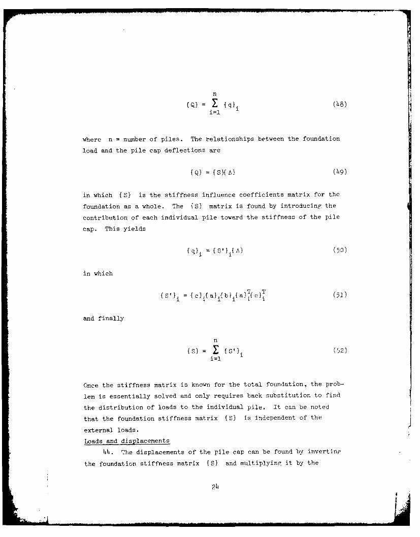
{QI = X {q~i (48)! i=l

where n number of piles. The relationships between the foundation

load and the pile cap deflections are

Q) SY s}A} (49)

in which {S} is the stiffness influence coefficients matrix for the

foundation as a whole. The {S1 matrix is found by introducing the

contribution of each individual pile toward the stiffness of the pile

cap. This yields

{q}i = {S'}i{A} (50)

in which

{S'} i ={c}ifa}i.bJi{a} Tc I(51)

and finally

n

{S}= {s,. (52)i=l

Once the stiffness matrix is known for the total foundation, the prob-

lem is essentially solved and only requires back substitution to find

the distribution of loads to the individual pile. It can be noted

that the foundation stiffness matrix {S) is independent of the

external loads.

Loads and displacements

4h. The displacements of the pile cap can be found by inverting

the foundation stiffness matrix {S) and multiplying it by the

24

external load matrix { Q} or

fA} = {S}-{Q} (53)

Once the foundation deflections are known the deflection of pile i

about its own axes can be found by

T T1 1 1

Finally, the forces allotted to each pile about its axes can be found

from Equation 1 where

fF}. = {b}.{x}. (55)1 1 1

It may be desirable to resolve the forces along the pile axes to forces

parallel to the structure coordinate axes. These can be found by

F f a}.{b).a).{cl.(A} (56)

Failure Criteria

Allowable loads

45. The allowable axial loads for combined bending (ACB), the

allowable moment about the minor principal axis (AMIN), Ind the allow-

able moment about the major principal axis (AMAJ) differ in prestressed

concrete piles depending on whether the pile is in tension or compres-

sion. Therefore, the program allows the user to input two sets of

values for the above-mentioned variables, one set for piles in tension

and one set for piles in compression. The program checks whether the

value of the axial force in the pile is positive (compression) or

negative (tension) to determine which set of allowables will be used

25

for checking failure. The program also allows the user to input an

allowable compressive load and an allowable tensile load.

Combined bending factor

46. The combined bending factor for a three-dimensional case is

computed as (a) the absolute value of the vertical pile force divided

by the allowable axial load plus (b) the absolute value of the moment

about the U axis divided by the allowable moment about the minor axis

plus (c) the absolute value of the moment about the U axis divided by2

the allowable moment about the major axis. The pile is considered to

fail if the combined bending factor is greater than one.

Buckling

47. The program calculates a buckling factor for a constant soil

modulus or a linearly varying soil modulus. For a constant soil modulus

the buckling factor is

PBUCK = (7 x DF x (1 + PR) x E x AMIN) x E), x E)) (57)56.0 ((Il Es 2 s (

where

DF = degree of fixity

PR = pile resistance (end bearing or friction)

E = modulus of elasticity of pile material

AMIN1 = minimum of two values in parentheses

X = pile dimension parallel to Ul-axis of the pile

48. For a linearly varying soil modulus the buckling factor is

2.0

PBUCK =7 x DF x (l + PR) x 1.57 x Es

(58)

S 3.0 (2.0 ~ 3.0 ~20 T3.)× E3O xAMIN1 (X 13" 2 . 0 x2.) "

h9. A pile fails in buckling if the buckling factor, PBUCK , is

greater than zero and less than the axial force in the pile.

26

Compression and tension

50. If a pile is in compression, it fails when the allowable

compressive load is exceeded by the axial force in the pile. If a

pile is in tension, it fails when the allowable tensile load is

exceeded by the absolute value of the axial force in the pile.

27

PART IV: USER'S GUIDE FOR PROGRAM LMVDPILE

General Introduction

51. Documentation for the computer program LMVDPILE (analysis of

two- and three-dimensional pile foundations) is presented herein and in-

cludes a general introduction, program listing, flow charts, guide for

data input, and input-output data for several example problems.

52. LMVDPILE is a general direct stiffness analysis computer

program that can be used to determine structure deflections, pile de-

flections, and forces acting on a group of piles placed in soil and

topped with a rigid cap.

53. In the analysis used in LMVDPILE, the base (pile cap) is

assumed to be rigid, and the structure and soil are considered to behave

in a linear-elastic manner. Each pile behavior in a three-dimensional

problem is represented by a 6 by 6 stiffness matrix and in a two-

dimensional problem by a 3 by 3 stiffness matrix (Hrennikoff 1950, Saul

1968). The elastic pile constants b are dependent on many factors,

as shown in Part III, and can be obtained by using the sets of equations

given. The direct stiffness method is then used to analyze the problem.

5h. Two companion programs are available for use with LMVDPILE.

One is a preprocessor routine (PILESTF) which will calculate the pile-

head stiffness matrix bij for a pile in layered soil with a lateral

subgrade modulus E varying with depth as follows:5

E= K + K2zn (59)

where

z = depth

Ki, K2 9 n = soil parameters

When K2 equals zero, Es is a constant (such as for clays). When

K1 equals zero and n equals 1.0, Es is linearly varying (such as

for sands). The pile-head stiffness can be used as input to the LMVD-

FILE program. Documentation for PILESTF is presented in Appendix A.

28

55. The second program is an interactive graphics postprocessor

display program (FDRAW). Program LMVDPILE writes an output file which

is used by FDRAW to display geometry, batter, pile loads, and load

factors as calculated by program LMVDPILF. Documentation for FDRAW is

presented in Appendix B. A pile optimization program that can help in

designing pile layouts is also being developed.

56. LMVDPILE can be run on the WES G-635, Macon H6000, and Boeing

CDC computers in the time-sharing mode. The program is part of the

CORPS (Conversationally Oriented Real-Time Program-Generating System)

library. It is identified by the program number X0034. To execute the

program, issue the appropriate run command given below:

a. On the WES or Macon computer

RUN WESLIB/CORPS/XOO3h ,R

b. On the Boeing computer

OLD,CORPS/UN=CECELB

CALL, CORPS ,XO03h

Data may be input interactively at execute time or may be input as a

prepared data file. Output may be directed to an output file or come

directly back to the terminal.

Flow Charts

57. A flow chart for the program is shown in Figure 4. The

sequence of operations for subroutine BMAT, a subroutine to calculate

elastic pile constants, is diagrammed in Figure 5.

Data Input for LMVDPILE

58. Data input to program LMVDPILE is basically the same for a

two- or three-dimensional analysis. However, for the user's convenie nce,

the data input guide for a two-dimensional analysis is given first.

Then the data input guide for a three-dimensional analysis is riven.

Guide for two-dimensional data input

59. Data for a two-dimensional analysis should be input to program

29

MAIN PROGRAM LMVDPILE

INPUT TITLE

INPUT NUMBER OF PILES (NP), PILEGROUPS (NPG), LOADING CONDITIONS (NLC)

CALL BMAT - SUBROUTINE TOCALCULATE ELASTIC PILE CONSTANTS

r DO FOR EACH PILE, IP =1, NP

COMPUTE C-MATRIX COORDINATESI I

I COMPUTE A- MATRIXBATTER AND ANGLE ORIENTATION

IMULTIPLY C-MATRIX TIMEA- MATRIX = CA

MULTIPLY CA-MATRIX TIMESI B- MATRIX =CAB

I MULTIPLY CAB-MATRIX TIMES TRANSPOSEOF CA-MATRIX = SI MATRIX (STIFFNESS)

L CONTINUE

A

Figure 4. Flow chart for LMVDPILE (sheet 1 of 2)

30L__

S COMPUTE FLEXIBILITY MATRIX

S = INVERSE OF STIFFNESS MATRIX

COMPUTE COORDINATES OFELASTIC CENTERS

IDO FOR EACH LOADING CONDITION

DOFR LC =1,NLC

I INPUT APPLIED LOADS Q- MATRIX

I COMPUTE STRUCTURE DEFLECTIONSD = S (FLEXIBILITY) *Q (LOADS)

I ~ 4DO FOR EACH PILE IP =1,NP JI II I COMPUTE PILE DEFLECTIONS ALONG

I IPILE AXIS Q CAT * DI if COMPUTE PILE FORCES ALONG PILE

I AXISQ:SI *DJ

I ( CHECK PILE FOR FAILURE

I [ COMPUTE PILE FORCES ALONG STRUCTUREI AXIS D = A (ANGLE ORIENTATION) * Q

(PILE FORCES ALONG PILE AXIS)

CONTINUE

Figur 4 (s.CONTINUE

Figure 4 (sheet 2 of 2)

SUBROUTINE BMATI] DO FOR EACH PILE GROUPI- INPG 1,NPG

INPUT PILE GEOMETRIC,MATERIAL, &

FIXITY PROPERTIES

COMPUTE B-MATRIX ELASTICFigure 5. Flow chart of sub- PILE CONSTANTS

routine BMAT for LMVDPILE _

INPUT ALLOWABLE LOADS &

MOMENTS

L CONTINUE

RETURN

LvVDPILE according to the following guide. All input is in free field

(a comma or at least one blank should separate data items). Data can

be input either interactively or from a data file. If a data file is

created, use line numbers for each data line.

Group 1 - Title

A. TITLE

TITLE = 66-character problem heading

B.1 TITLE1

TITLEI = second 66-character problem heading

Group 2 - Control Data for Piles and Loads

A. ITYPE

ITYPE = code for type of analysis2 --- two dimensional

B. NP, NPG, NLC

NP = number of pile rows

32• A

NPG = number of pile groupsNLC = number of loading conditions

Group 3 - Control and Data for Soil Properties

MV ES

MV = type of soil modulus variance1 --- constant soil modulus2 --- linearly varying soil modulus

ES = subgrade modulus (units are in psi) for MV = 1ES = KS = coefficient of subgrade modulus (pci) for MV = 2

Group 4 - Control and Data for Elastic Pile Constants

Note: Groups 4-8 should be repeated NPG (number of pile groups)number of times.

A. NPA, NPB, SLEN, NPS

NPA = identification number of first pile in pile groupNPB = identification number of last pile in pile groupSLEN = length of pile (feet)NPS = code for type of input to compute elastic pile con-

stants (B-matrix terms)1 --- input B-matrix terms directly

2 --- any shape pile3 --- round pile

B. Note: Necessary only if NPS = 1

Bll B22, B33, B31

BIJ = elastic pile constant for row I, column J

C. Note: Necessary only if NPS = 2

SAIX, AIY, AREA, X, Y

AIX = II, moment of inertia about local U 1 axis (in. 4

AIY = 12, moment of inertia about local U2 axis (in. 4 )AREA = cross-sectional area of pile (in. 2 )

X = pile dimension parallel to U1 axis (in.)

Y = pile dimension parallel to U2 axis (in.) 2i

D. Note: Necessary only if NPS = 3

D

D = average diameter of piles in the groups (in.)

Group 5 - Control and Data for T'ile MaterialA. MP

T= type of materialI --- concrete (F calculated from I'S input in item 5B)

I.!.. ...... ... ............

2 --- timber (E set to 1,760,000 psi*)3 --- steel (E set to 29,000,000 psi)4 --- special (E input in item 5C)

B. Note: Necessary only if MP = 1

us W

US = ultimate strength of concrete (psi)W = weight of concrete (pcf)

C. Note: Necessary only if MP = 4

E

E = modulus of elasticity (psi)

Group 6 - Control and Data for Fixity Coefficients to Describe Pile

A. NF INF = code for input of fixities

1 --- input degree of fixity and all coefficients2 --- input degree of fixity

B. Note: Necessary only if NF = 1. See paragraph 35.

S, K1, K2, K3, K4, K5, K6

DF = degree of fixity of pile head-to-base (values between0 and 1)

K1 = lateral fixity coefficientK2 = pile axial resistance coefficient

1.0 --- end bearing pile in compression

2.0 --- friction pile in compression

For piles in tension the value should be reduced.

Suggest ore half of value for compression piles.

K3 = rotational fixity coefficientK4 = coefficient for torsionK5 = fixity constantK6 = fixity constant

C. Note: Necessary only if NF = 2

DF, PR, PFT, G

DF = degree of fixity of pile head-to-base (one of the threevalues given below)0.0 --- hinged pile head

0.5 --- partially fixed pile head

1.0 --- fixed pile head

A table of factors for converting U. S. 'ustomary units of measure-ment to metric (SI) units is presented on page

34

PR pile axial resistance coefficient, K21.0 --- end bearing pile in compression2.0 --- friction pile in compression

For piles in tension the value should be reduced.Suggest one half of value for compression piles.

PFT = participation factor for torsion, Kh (values between0 and 1) (equals zero for 2-D problem)

G = torsion modulus (psi) (equals zero for 2-D problem)

Group 7 - Data for 2-D Analysis (ITYPE = 2)

NROW

NROW = number of similar rows

Group 8 - Data for Allowable Pile Loads and Moments

ACL, ATL, ACB, AMAJ

ACL = allowable compressive load (kips)ATL = allowable tensile load (kips)ACB = allowable compressive load in bending (kips)AMAJ = allowable moment (kip-ft)

Note: Repeat groups 4-8 data NPG (number of pile groups)number of times.

Group 9 - Control and Data for Pile Orientation

A. FIB

IB = code for input of batter and angle0 --- input batter and angle for each pile

>0 --- number of subgroups of piles in the group withthe same batter and angle orientation

B. Note: Necessary only if IB (number of subgroups) > 0Repeat IB number of times.

INFP, NLP, BATT

NFP = identification number of first pile in subgroupNLP = identification number of last pile in subgroup

BATT batter "BATT" vertical on 1 horizontal<0 --- pile slopes from top right to lower left

=0 --- vertical pile

>0 --- pile slopes from top left to lower right

Group 10 - Pile Data for 2-D Pile Groups (ITYPE=2)

Note: Necessary only if IB > 0

Ul(1) Ul(2) Ul(3) U(NP)

35

L

* U1 = distance from origin to pile along Ul-axis.

Group 11 - Data for Pile Orientation

Note: Necessary only if IB = 0 and ITYrE = 2 (2-D pilegroups). Repeat NP (number of pile rows) number oftimes

H, Ul

H batter H vertical on 1 horizontal<0 --- pile slopes from top right to lower left0 --- vertical pile

>0 --- pile slopes from top left to lower rightUl distance from origin to pile along U1 axis (feet)

Group 12 - Data for applied Loads and Moments

Note: Repeat NLC (number of loading conditions) number oftimes.

q1 = horizontal load along U1 axis (kips)Q3 = vertical load along U axis (kips)Q5 moment about U2 axis kip-ft)

Guide for three-

dimensional data input

58. Data for a three-dimensional analysis should be input to pro-

gram LMVDPILE according to the following guide. All input is in free-

field (a comma or at least one blank should separate data items). Data

can be input either interactively or from a data file. If a data file

is created, use line numbers for each data line.

Group 1 - Title

A.1 TITLE

TITLE 66-character problem heading

B. TITLE1

TITLE1 second 66-character problem heading

Group 2 - Control Data for Piles and Loads

A.1 ITYPE

Successive piles with the same coordinate may be input in the form:

N*U

where N = the number of piles with the same coordinates

U = the value of the coordinate in feet

36

ITYPE code for type of analysis

3 --- three dimensional

B. NP, NPG, NLC

NP = total number of pilesNPG = number of pile groupsNLC = number of loading conditions

Group 3 - Control and Data for Soil Properties

MV, ES

MV = type of soil modulus variance1 --- constant soil modulus2 --- linearly varying soil modulus

ES = subgrade modulus (psi) for MV = 1ES = KS = coefficient of subgrade modulus (pci) for MV 2

Group 4 - Control and Data for Elastic Pile Constants

Note: Groups 4-7 should be repeated NPG (number of pile groups)number of times.

A.1 NPA, NPB, SLEN, NPS

NPA = identification number of first pile in pile groupNPB = identification number of last pile in pile groupSLEN = length of pile (feet)

NPS = code for type of input to compute elastic pileconstants (B-matrix terms)1 --- input B-matrix terms directly2 --- any shape pile

3 --- round pile

B. Note: Necessary only if NPS = 1

Bll B22, B33, B44, B55, B66, B42, B51

B11, etc = elastic pile constants

C. Note: Necessary only if NPS = 2

AIX, ATY, AREA, X, Y

AIX = I,, moment of inertia about local U1 axis (in. )

AIY = I, moment of inertia about local U2 axis (in. 4 )AREA cross-sectional area of pile (in.2

X = pile dimension parallel to U1 axis (in.)Y = pile dimension parallel to U2 axis (in.)

D. Note: Necessary only if NPS x3 (

0D N

D = average diameter of piles in the groups (in.)

37

Group 5 -Control and Data for Pile Material

A. MP

MP = type of material1 --- concrete (E calculated from US input in item 5B)2 --- timber (E set to 1,760,000 psi)3 --- steel (E set to 29,000,000 psi)4 --- special (E input in item 5C)

B. Note: Necessary only if MP = 1

us W

US ultimate strength of concrete (psi)

W = weight of concrete (pcf)

C. Note: Necessary only if MP = 4

E

E = modulus of elasticity (psi)

Group 6 - Control and Data for Fixity Coefficients to Describe Pile

A. NF ]

NF = code for input of fixitiesI --- input degree of fixity and all coefficients2 --- input degree of fixity

B. Note: Necessary only if NF = 1. See paragraph 35.

SDF, K K2, K3 4, K5, K6

DF = degree of fixity of pile head-to-base (values between0 and 1)

Kl = lateral fixity coefficientK2 = pile axial resistance coefficient

1.0 --- end bearing pile in compression2.0 --- friction pile in compression

For piles in tension the value should be reduced.Suggest one half of value for compression piles.

K3 = rotational fixity coefficientK4 = coefficient for torsion

K5 = fixity constant

K6 = fixity constant

C. Note: Necessary only if NF = 2

DF, PR, PFT, G

DF = degree of fixity of pile head-to-base (one of the threevalues given below)0.0 --- hinged pile head0.5 --- partially fixed pile head1.0 --- fixed pile head

38

PR = pile axial resistance coefficient, K21.0 --- end bearing pile in compression2.0 --- friction pile in compression

For piles in tension the value should be reduced.

Suggest one half of value for compression piles.

PFT = participation factor for torsion (values between 0and 1), K4

G = torsion modulus (psi)

Group 7 - Data for Allowable Pile Loads and Moments

ACBT, AMINT, AMAJT, ACBC, AMINC, AMAJC, ACL, ATL

ACBT allowable axial load used in combined bending equa-tion for pile in tension (kips)

AMINT = allowable moment about minor principal axis for pilein tension (kip-ft)

AMAJT = allowable moment about major principal axis for pilein tension (kip-ft)

ACBC allowable axial load used in combined bending e4ua-tion for pile in compression (kips)

AMINC = allowable moment about minor principal axis for pilein compression (kip-ft)

AMAJC = allowable moment about major principal axis for pilein compression (kip-ft)

ACL = allowable compressive load (kips)ATL = allowable tensile load (kips)

Note: Repeat groups 4-7 data NPG (number of pile groups) numberof times

Group 8 - Control and Data for Pile Orientation

A. iB

IB = code for input of batter and angle0 --- input batter and angle for each pile>0 --- number of subgroups of piles in the group with

the same batter and angle orientation

B. Note: Necessary only if IB (number of subgroups) > 0

NFP NLP, BATT, ANL

NFP = identification number of first pile in subgroupNLP = identification number of last pile in subgroupBATT = batter "BATT" vertical on 1 horizontal

0 --- vertical pileANGL = clockwise angle between the po:;itive U1 axis of the

structure and the U axis (direction of batter) of the

pile (degrees)

Group 9 - Pile Data for 3-D Pile Groups (ITYPE = 3)

39

Note: Necessary only if IB > 0.

A. 1 Ul) Ul(2), Ul(3),... Ul(NP)

* Ul = distance from origin to pile along U1 axis (feet)

B. U2(l), U2(2), U2(3),... U2(NP) .. .

* U2 = distance from origin to pile along U2 axis (feet)

C. U3(l), U3(2), U3(3),... U3(NP)

* U3 = distance from origin to pile along U3 axis (feet)

Group 10 - Data for Pile Orientation 3-D Pile Group (ITYPE = 3)

Note: Necessary only if IB = 0. Repeat NP (number of piles)number of times.

H, ANG, Ul, U2, U3

11 = batter H vertical on 1 horizontal0 --- vertical pileANG = clockwise angle between the positive U1 axis of the

structure and the U1 axis (direction of batter) ofthe pile (degrees)

Ul = distance from origin to pile along Ul-axis (feet)U2 = distance from origin to pile along U2 -axis (feet)U3 = distance from origin to pile along U 3-axis (feet)

Group 11 - Data for Applied Loads and Moments

Note: Repeat NLC (number of loading conditions) number of

times.

S Q3, Q, 5 Q6

Ql = horizontal load along U1 axis (kips)Q2 = horizontal load along U2 axis (kips)Q3 = vertical load along U3 axis (kips)Q= moment about U1 axis (kip-ft)Q5 = moment about U2 axis (kip-ft)Q6 = moment about U 3 axis (kip-ft)

* Successive piles with the same coordinate may be input in the form:

N*U

where N = the number of piles with the same coordinates

U = the value of the coordinate in feet

40

PART V: EXAMPLE PROBLEMSE

Example Problem 1

Two-dimensional problem, 2 pinnedpiles with constant soil modulus_

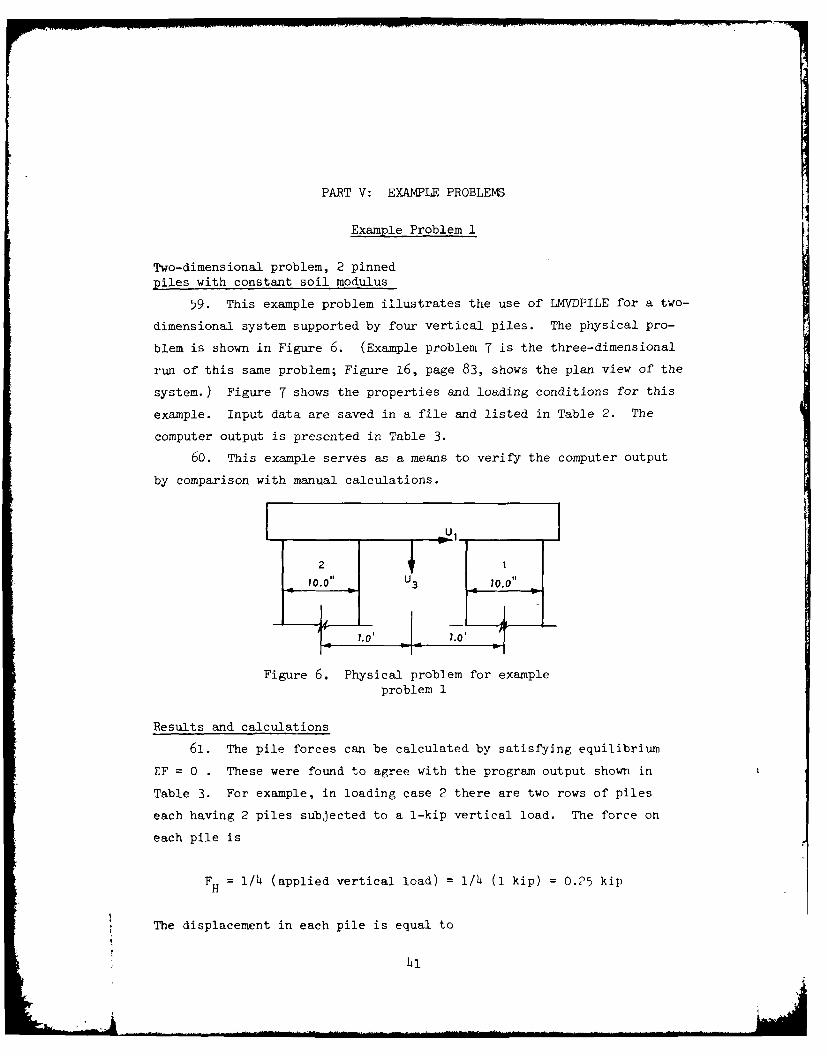
59. This example problem illustrates the use of LMVDPILE for a two-

dimensional system supported by four vertical piles. The physical pro-

blem is shown in Figure 6. (Example problem 7 is the three-dimensional

run of this same problem; Figure 16, page 83, shows the plan view of the

system.) Figure 7 shows the properties and loading conditions for this

example. Input data are saved in a file and listed in Table 2. The

computer output is presented in Table 3.

60. This example serves as a means to verify the computer output

by comparison with manual calculations.

21

10.0" U3 1.

1.01 1.0.

Figure 6. Physical problem for exampleproblem 1

Results and calculations

61. The pile forces can be calculated by satisfying equilibrium

E= 0 . These were found to agree with the program output shown in

Table 3. For example, in loading case 2 there are two rows of piles

each having 2 piles subjected to a 1-kip vertical load. The force on

each pile is

FH 1/4 (applied vertical load) =1/4 (1 kip) = 0.25 kip

The displacement in each pile is equal to

Properties

lt. str. of concrete = 5000.0 psi Vertical (h 0.0)

ES = 10.0 psi Degree of fixity = 0.0

I, = 833.333 in. Pile resistance (K2)4 = 1.0

12 = 833.333 in. Participation factor for

torsion (K4) = 0.0

Area = 100 in.2 Torsion modulus 0.0

Length = 100 ft

Loading Q1 2 Q3Case (kips) (kips) (kip-ft)

1 1.0 0.0 0.0

2 0.0 1.0 0.0

3 0.0 0.0 1.0

4 1.0 1.0 1.0

Figure 7. Properties and loading conditions for

example problem 1

42

Table 1

Interactively Input Data for Example Problem 1

INPUT DATA FILF NAMT I% CHAPACTrRS CR LFSS. fIT ACARRIAGE RETURN IF INPUF DtTA *ILL COME FROM T'RMINAL.

7

INPUT A FILE NAME FOR DATk. HIT A CARRIAGE ErURNIF YOU DO NOT WANT TO SAVE DATA FILF.

? DATA1

INPUT TWO LINFS OF PROJECT IDENTIFICATION NOTTO EXCEED 66 CHARACTERS EACF

INPUT FIRST LIN!7 EXAMPLF PROBL

r, jO. I

INPUT SECOND LINT7 VERTICAL PILNS I'i 'J'IT tZALL

DO YOU WANT TO RUN A 2-D OR 3-D ANALYSIS?ENTER 2 OR 3 7 2

INPUT TOTAL 4UMBER OF PILE ROWS IN FOUNDAIIONNUMBER OF PILE GROUPS AND LOADING CONDITIONS

7 2.1.4

INPUT SOIL PROPERTY DATA - MV AND FS:Y=I-CONSTANT SOIL OR MV-?-L:vEAPLY VAREIKI SOIL

rS-SUBGRADE MODULUS (PSI IF V-V1 OR PCI IF MV=2,1 .,0.9

DATA FOR PILr GROUP No. - 1

INPUT PILr SHAPE DAtA:NPA-IDENTIFICATION NUMR'R Or F'RS? P1h' RCW IN _RO;PNPB-IDENTIFICATION NUMBER OF LAST PILE RO I' G OUPSLFN-LINGTR OF PILES (FEET)NPS-CODE FOR TYP. OF INPUT TO COMPU:F r TIIIC PILE, CCNSTANTS

1=INPUT PILE B MATRIX TE;MS DIRrCTLY2-ANT SHAPE PIL?3-4OUND PILE

? 1.2,104.0.2

INPUT AIX & AIT-'iO"NTS OF INERTIA iN**4)AREA - CROSS SECTIONAL ARFA (IN**2)I & T - PIL7 DIMENSIONS ALONG X & I AXES INCNP.

7 833.333,933 .3 IZ.OI .0,lZ.e

INPUT PILt MATERIAL DATA-IF tjIO'.CvrTF. q-'I"AER. T:STrtL, 4:SPTCIAL;?1

INPUT US=ULTI1ATF STRINIT" OF CONC-'T1 7?d-W!IGHT OF CO%,RETE (PCF)

? 500.0.9.l.e

INPUT FIXITY DATA - NF (1-INPUT ALL FIXITY CCrFICIE4TOR 2=INPUT DrGREE OF FIXITY

?2

INPUT DF - DTGRTE OF FIXITY )[email protected],1.B)PP - PILV R

TLISrAN^E (0ABI' , . ICTIO

PFT - PARTICIPATION FACTO- FOR TCREIC'.G - TORSION MODILUS (PSI)

(Continued)

Table 1 (Concluded)

INPUT NUMBFR Ci SIMILAR ROiS IN G3 OI 1 ? 2

INPUT ALLOABIT LOADS:ACL ALLOABIF COMPRESSIVE IA, .KIS,ATL ALLOWABL7 TENSILE LOAD FiP~AC3 ALLOWAbLE COMPRFSSI1E LOAD IN BiNDIN3 (KIiS)AMAJ AILOABLT MOM-NT ) IP-FT,

? le. a. ea.h. 10.0. Hu.0

INPUT I: 4=INPUT BATTYR FOP EAC) PIL, CRTilF NUMBPR OF SUBGROUPS WITH TAE SAMF EATTEP

? 0

INPUT PILE ORITNTATION DATAH-BATTFF=H VERTICAL ON I FORIZONTALPOSITIV7 IF BATTERED TO RI~nT :!EGATIVF I- o L',Ul=DISNCI FRO- ORIGIN TO PILr ,04(FET)

1 7 o.e.1.02 ? . ,

INPUT APPLIED LOADE AKD MOPEKT:01-BORIZONTAL LOAD ALONG Ul-AXIS EIPSI03-VERTICAL LOAD ALONS U3-AXIS (KIPS)Q!-MOMEN? A OUT U2-AXIS (IIP-FrEC,

FOR LOADING CONDITION - 1 7 1.0,6,0

FOR LOADING CONDITION - 2 ? 0,1.0,e

FOR LOADING CONDITION - 3 ? 0.0.1.2

FOP. LOADING ONDITION - 4 ? 1.2,1.2.1..

TIllS PROGRAM GEERATES THT PCLLg4IN; TAOLFS

TABLE NO. CO%TYNTS1 PILr ANI SOIL DATA2 PILE COOPEICArrS i.D 3TT-i3 STIFFNESS AtD FLE(Ihlt:T1 MAT'.ES FL IRI

STRUCTURF AND :OORDINATrS OF ELASTIC CV'TEh4 APPLIED LOAPS5 srRUCTURr DEFLECTIOnS

6 PILE DEFLFCTIC4S ;LONG Flit AXIS7 PILE FORCES ALONG PILE AXlS

8 PILE FORCES ALONG STRUCTURT AXIS

INPUT TFE NUMBVRS OF THE TABLES FOR WHICH YOU WANT THE OJTPUT.SEPARATE THE NUMBERS WITH COMMAS. ? 1,2,3,4,5,6.7,8

INPUT A FILENAME FOR TABLE 8 IN q CHARACTYRS OP LESSIF YOU WANT TO Sr THIS INFORMATION FOR A iW .J1,BIT A CARRIAjr RVTURN ID YOU DO NOT WAIV TYIIS FILE.

7

INPUT A FILE NAME FOP OUTPUT I% CRAPACTFFS -S :5.

HIT A CARRIAGr

RrTUR% IC OUTPUT IS TO RE V?'I'TFD ON TP1INkL.?

INPUT A FILE NAME IN ' ChARACTerS OR iSS FR POC .utA EyCr$S:TFOB PROGRAM FDRAd. HIT A CARRIAGE RrTURN IF TOJ DO NOT &A'iU TO

SAVE THIS FILE?

44

Table 2

Input Data for Example Problem 1

(,roup1A 10000 EXAMPLE PROBLEM NO. I1B 10010 VERTICAL PILES WITF UNIT LOADS TITLE2A 10020 2 12-D ANALYSIS2B 10030 2 1 4 INUMBER OF PILES. PILE GROUPS, LOADING CONDITIONS3A 10040 1 10.000 FSOIL PROPERTIES]h-A 1-0050 1 ? 100.000 2 TPIE GEOMETRY

hc 10060 833.333 833.333 100.000 10.000 10.0005A 10070 15B 10080 5000.000 150.000 JPILE MATERIAL6A 10090 26c 10100 0. 1.000 0. 0.

110 ? NUMBER OF ROWSI8 10120 100.000 100.000 100.000 100.000 [ALLOWABLE LOADS

--- A 10130 011 10140 0. 1.0910 IPILE BATTER AND LOCATIO

10150 0. -1.00010160 1.000 0. 0.

12 10170 0. 1.000 0. [APPLIED LOADINGS10180 2. 0. 1.00010190 1.000 1.000 1.000

45

Table 3

Output Data for Example Problem 1

EXAMPLE PROPLTM NO. IVERTICAL PILES WITH UNIT LOADS

NO. OF PILE ROWS - 2 P MATRIX IS CALCULATED FOR EACH ROW

1. TABLE OF PILE AND SOIL DATA

PILE NUMBERS

I 2 B - 0.43r 07 PSI It - 833.33 IN**4 IT - 833.33 IN**4AREA - 100.0 IN't2 X = 10.00 I' T = 10.00 INLENGTH - 100.0 FPET ES - 10.000TI = 0.4107 12 = 1.0000 13 = 0.K4 - 0. K5 - 0. X6 = 0.

ALLOWABLES: COMPRESSIVE LOAD - 100.000 KIPSTENSILE LOAD - 100.000 KIPSBINDING - 100.000 KIPSMOMENT - 100.000 KIP-FT

THE B MATRIX FOR PILES 1 THROUGH 2 is

0.972E 03 0. 0.0. 0.357E 06 0.0. 0. 0.

2. TABLE OF PILE COORDINATES AND BATTER

PILE ROW BATTER Ut (FT)1 VERTICAL 1.0002 VERTICAL -1.000

3. STIFFNESS MATRIX S FOR THE STRUCTURE

0.3893 04 0. 0.0. 0.143F 37 0.0. 0. @.Mr6 09

3A FLEXIMILITT MATRIX 7 FOR THE STRUCTURE

0.2572-03 0. 0.0. 6.1Y99-06 0.0. e. 0.48fr-08

COORDINATES OF ELASTIC CENTERtc1 0. IC2 - 0.

(Continued) (Sheet 1 of 5)

46I

Table 3 (Continued)

LOADING CONDITION I

4. MATRIX OF APPLIED LOADS Q (KIPS & FEET)

Q1 03Vi.00 0. 0.

DI D3 D50.257E 00 .0

6. PILE DEFLECTIONS ALONG PILE AXIS (INCHES)

PILE X1 X1 X51 0.257E 00 0. 0.2 0.257E 00 0. 0.

7. PILE FORCES ALONG PILE AXIS (KIPS & PT)

PILE E1 PS 75 VAILUREEU CO TE

1 0.250 0. 0.2 0.250 0. 0.

TOTAL NO. FAILURES - 0 LOAD CASE I

8. PILE FORtCES ALONG STRUCTURE AXIS (KIPS & FEE?)

PILE Fl 73 F51 0.250o 0. 0.2 0.250 0. 0.

sum 1.000 0. 0.

(Continued) (Sheet 2 of 5

47V

Table 3 (Continued)

LOADING CONDITION 2 ******

4. MATRIX OF APPLIED LOADS 0 (KIPS & FEET)

0. 1.200 0.

5. STRUCTURT DEFLECTIOS (INCHES)

DI D3 D50. 0.7001-03 0.

e. PILE DEFLECTIONS ALONG PILE AXIS (INCHES)

PILE X1 X3 ES

1 0. 0.700-03 P.2 0. 0.70')-0 0.

7. PILE FORCES ALONG PILE AXIS (KIPS & FT)

PILT El 13 F5 'AILUREPI c0 TE

1 . .2!;o 0.2 0. 0.2"C 0.

TOTAL NO. FAILURES - 0 LOAD CASE 2

S. PILE FORCES ALONG STRUCTURE AXIS (KIPS FET)

PILE 1 75 T51 0. 0.250 0.2 0. 0.25? 0.

SUM 0. 1.200 -0.080


48

Table 3 (Continued)

******** LOADING CONDITIO4 3 *******


QI 03 Q53. 0. 1.000

5. STRUCTURE DEFLECTIONS (INCORS)

D1 D3 DF0. 0. 0.583T-14

E. PILE DEFLECTIONS ALONG PILE AXIS (INCHES)

PILE X1 X3 X51 0. -0.700W-03 0.583v-41 0. 0.700E-33 0.583E-04

7. PILF FORCES ALONG PILE AXIS (KIDS & FT)

PILE F1 F3 F5 FAILUqEPU CO TE

1 . -0.2 ? 0.? 0. P.2 P 0.

TOTAL NO. FAILURTS - 0 LOkD CASE 3

S. PILE FORCES ALONG STRUCTURE AXIS (KIDS & FEET)

PILF F1 F1 F

1 0. -0.2!' 0.? P. 0.259 0.

SUM 0. 7. 1.000

(Continued) (Sheet of 5)

49

Table 3 (Concluded)

LOADING CONDITION 4 *

4. MATRIX OF APPLIED LOADS Q (KIPS FEET)

Ql 03 Q5

1.000 1.000 1.000

5. STRUCTURE DEFLECTIONS (INCHES)

D1 D3 D50.257E 00 0.700E-03 0.583E-04


PILE X1 13 X9I 0.257E 00 -0.364E-11 0.5q3E-042 0.?57T 00 0.140,-02 0.583E-04

7. PILE FORCES ALONG PILE AXIS (KIPS TT)

PILE F1 F3 F5 FAILUREPu CO ?I1 0.713 -0.000 0.2 0.253 0.!00 0.


S. PILE FORCES ALONG STRUCTURE AXIS (KIPS ( FEE?)

PILE F1 F3 751 0.260 -0.P00 0.

2 0.150 0.00 0.

SUm 1.000 1.000 1.000

(Sheet 5 of 5)

50

1PL = x 1 x 100 x 12 -03

6 = 0.P7 l 10 in.AE 4300 x 1 44 x 100

1144

This result also agrees with the computer program results (page 48,

item 6).

62. In loading case 3, a 1 kip-ft moment is applied about the

U 2-axis. The pile forces can be calculated by satisfying equilibriumEm2 0

Em 2 = F31 x N U11 + F32 x N x U12 + Q5

where

F3 = vertical force for pile row m, m =1,2m

N = number of piles in rows

U1 = distance from origin to pile

:.Em2 = 2F31 + 2F32 + 1 kip-ft

From symmetry F31 = F32

.IF31 = 0.25 kip

This result also agrees with the computer program results (page 49,

iter 8).

63. Load case 4 can be obtained as a superposition of load cases

1 through 3. The deflections of the pile and the load on each pile can

be obtained by [uperimposing the respective results for load cases 1

through 3. The following computations verify these results.

51

Deflections

No. Case X1 (in.) X3 (in. x5 (rad.)

1 1 0.257 0. 0.2 . 0.7 x 0- 3 0.

3 0. -0.7 x 10 0.583 x 10

4 0.257 0. 0.583 x 10- 4

(page 50, item 6)

2 1 0.257 0. 0.2 0. 0.7 x 10-3 0.3 0. 0.7 x 10 0.583 x 10

4 0.257 0.114 x 102 0.583 x lo(page 50, item 6)

LoadsF (kips) F3 (kips) F5 (kip-ft)

1 1 0.25 0. 0.2 0. 0.25 0.3 0. -0.25 0.

4 0.25 0. 0.(page 50, item 7)

2 1 0.25 0. 0.2 0. 0.25 0.3 0. 0.25 0.

4 0.25 0.50 0.(page 50, item 7)

These results also agree with the computer program results.

5

*11

52

Example Problem 2

Two-dimensional prob-lem, 1 fixed vertical pile

64. This example problem has only one vertical pile completely

fixed into the rigid cap. Figure 8 shows the physical problem. (Exam-

ple problem 8 is the three-dimensional run of this same problem; Figure

19, page 96, shows the plan view for this example.) Figure 9 shows the

loading and properties. The input data are stored in a file and are

presented in Table 4. The computer output is shown in Table 5.

65. This example is also a means to verify output by comparison

with manual calculations and output from example problem 8.

I KIP-FT

U3

Figure 8. Physical problem for example problem 2

PropertiesUlt. str. of concrete = 5000.0 psi K1 = 1.0756

KS = 10.0 pci DF = 1.0 K2 = 1.0

I, = 833.333 in. PR = 1.0 K3 = 1.49881 143

12 = 833.333 in. PFT = 0.0 K4 = 0.0

Area = 100.0 in. G = 0.0 K5 = 0.9990

Length = 100.0 ft K6 = 0.9990

Vertical (h = 0.0)

Loading Ql 5Case (kips) (kips) (kip-ft)

1 0.0 0.0 1.0

Figure 9. Properties and loading for example problem 2

3

Table 4Input Data for Example Problem 2

Group1A 10000 EXAMPLF PROBLFM O. ?lB 10010 ONE FIXED VEPTIZAL PILr WITH 'NIT MOM'NT APPLIED2A 100-20 22B 10030 1 1 13 10040 ? 10.000hA 10050 1 1 100.000 24c 10060 P33.733 833.333 100.000 10.000 10.V005A 10070 15B 10080 f;000.300 157.0006A 10097 26C 10100 i.e3 1 .000 0. 9.7 10110 18 10120 10Z.000 100.007 100.000 110.0009A 10130 0

Ii 10140 0.•

12 10150 0. 0. 1.00

524

Table 5


eitEPHORLtM1 NJ. 20.2 HEEL ViRTIIAL PIU! aI7H UNIT MJ).'INT AFPLLED

NO2. OF PILE ?JdS 1 1 'ATFHE IS 2'ALCJLA7ED FOR EACH SCs

1. T~oLE OF ?ILi AND SOIL. DATA

PILE NJ'IoEPS

1 1 L- = Z.43i 07 PSI Ix = 1,3.,3 , -4 IY = 3,3.33 IN**4AREA l 0e.4 1,,**2 9 1 ./0 IN 9 = 1.20 IN.LERIUrn = 101.0 FEET ES = 10.00/Kl 1.0756 £2 1.0o 62 1.4938£4 K 0. 05 .z990 K.6 Z .9990

ALL~dAoLES: CDM?RESSIRE LOaD 100.200 KIPSTiN3ILE LOAD I 00.0 IFsDEI.DINL 100.200 ,IPSMJML.NT 1?0.21/El-C

TiC L 'ATHE FOR PILta 1 Ti:O 09>1 1 1

Z2249 05 e. 0.1352- 070. 0.357! e6 0.0.135&. 07 2. 0.104! 09

2. TABLE OF PILE COORDINATES AND FATTER

FIME HO& 6ATTLE ii (FT)1 VERTICAL 2.

,5. STIFFNESS MAlk:X S FUR lIRE STriU.TJRF

0.25,4E 05 0. 0.115. 070. 0.357F of 0.0.135-E 27 e. 0.114E /9-

JA LLEEIEILIIT MATRIX F FOR TICE STRJCTUAiE

2..2-E-04 0. -. 10FV0. 0.2+3oi-05 0.

-0.12zi2-05 1. .Z2Z-07

COORD)IATES OF ELA5TIC CENTER21= 0. &.C2 - V.013

(Continued)

55

Table 5 (Concluded)

LOADIN; CONDITION 1 *

4. MATRIX Of APPLIED LOADS Q (KIPS & FEET)

01 Q3 Q50. 0. 1.Z00

5. SIRUTURE DEFLECTIONS (INCHES)

Di DC 05

E. PILL DEFLECTIONS ALONG Fli AXIS (INCqES

PILE xi X3 X51 -3.144E-il 2. 00F3

7. PILE JACES ALOG FL. AXIS (SIPS S FT;

FILL il i.3 F5 FAILUFEbEU CC 7E

IJTAL NO. iAILJ S - 0 LJAD CASE I

i ******************s***as*t*a*ss*********sss*ss*s ****** ******* ****.

i. PILE FJRCLS ALONG STRJZTJRi AXIS (KIPS & 1)11)

FILE F1 F3! F51 Z.Zze ?. 1.600

I. 1.20,e z. 1.9BQ

56 AlI


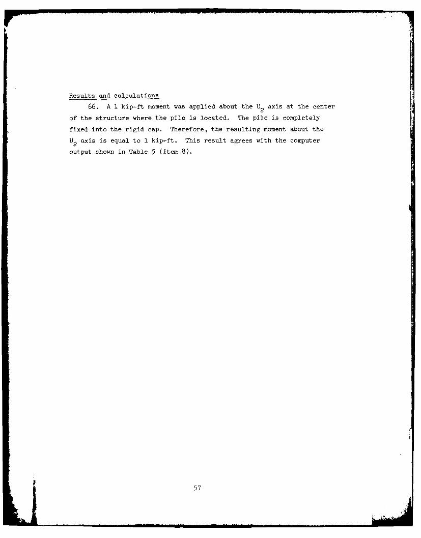
66. A 1 kip-ft moment was applied about the U2 axis at the center

of the structure where the pile is located. The pile is completely

fixed into the rigid cap. Therefore, the resulting moment about the

U2 axis is equal to 1 kip-ft. This result agrees with the computer

output shown in Table 5 (item 8).

57

Example Problem 3

Wo-dimensional problem,Hrennikoff' s examplecase 2a (very weak soil)

67. This example problem is taken from Hrennikoff's (1950) paper,

case 2a. This example is for very weak soil with hinged piles. The

physical problem is shown in Figure 10. The properties and loading

conditions are snown in Figure 11. The input data are stored in a file

prior Lo the run and are presented in Table 6. The computer output is

shown in Table 7.


with the classical method.

5.0 ' 3.0 -- U'

-* U

Figure 10. Physical problem for examples 3, 4, and 5


69. In Hrennikoff's paper manual calculations for this probleir

are presented. The computer results shown in Table 7 agree closely wlith

his results. A comparison of the two results is presented below. Por

pile 1,

FI = o.442 kips F3 = 27.395 kips

as compared with

F = o.44 kips F = 27.5 kips

519

Properties

E = 0.15 x 10 psi Degree of fixity 0.0

ES = 3.123 psi Pile resistance (K2)

4 =0.5I = 322.06 Participation factor

for torsion (K4)

4 =0.012 322.06 in. Torsion modulus 0.0

.2Area = 63.5 in.

Length = 30 ft

Loading Q1 Q3 Q5Case (kips) (kips) (kip-ft)

1 -39.375 113.1 173.41

Figure 11. Properties and loading conditions

for example problem 3

from case 2a in Hrennikoff's paper. Pile forces along the pile axis for

piles 2-5 also agree closely as tabulated below.

Hrennikoff'Computer Output Example

Pile F1 F3 FI F3

No. (kps ki s (kips) (kips)

1 o.14142 27.395 o.414 27.5

2 0.435 39.282 0.43 39.3

3 0.h27 51.170 0.43 51.0

4 0.436 -9.167 0.43 -9.0

5 0.436 lo.881 0.43 10.9

59

Table 6


Group1A 10000 EXAMPLE PROBLEM NO. 3lB 10010 HRENNIKOFF'S EXAMPLE - CASE 2A2A 10020 22B 10030 5 1 13 10040 1 3.1234A 10050 1 5 30.000 34D 10060 9.0005A 10070 45C 10080 1500000.0006A 10090 26C 10100 0. 0.500 0. 0.7 10110 18 10120 82.000 40.000 100.000 100.0009A 10130 29B 10140 1 1 -3.000

10150 4 5 0.10 10160 -5.000 -2.500 0. 3.000 7.00012 10170 -39.375 113.1 173.4

6o

Table 7


RUMPLE PROBLEM NO. 3iRENUIKORP'S LXIAPLI - CASE 4A

MO. O PILL IOWS - 5 A MATRIX IS CALCULATED FOR IAC6 ROW

1. TABLI Of PILE AND $OIL DATA

PILE NUMBlIS

5 S - 9.lb 07 PSI IX - 322.06 INS*A 1 - 322.06 IN**4AREA - 63.6 IN*02 = W.60 IN I = 9.00 INLILNGTh - 3 0. PMT E4 = 3.123

K1 9 0.4 10?12 0 - we0 1--= 0.£4 . 0. . o 0.

LENGTH Of PILES 38.df E T) IS INSUIFICIZNTPOR PILL GROUP - I MINIMUM aCCEPTABLE LEN3,TH IS 37.17 PEUTPOR SIMI-ININITI BSAM ON ELASTIC YOUNDATION

ALLOWABLIS: COMPhESSIVE LOAD 82.898 KIPSTNSIL- LOAD .0.060 KIPS

THE B MATRIX ]OR PIL4S 1 TROUGI H ISi

0.2461 03 0. 16.0. 0.133L 06 0.0. 0.l ~ 0.

2. TABLE OF PILE COORDINATE AND BATTER

PILL RO6 BATTh.R . (0T)1 -.. 00 -0.002 - 0-2 bee3 -3.1; 0.

4 YATZCAL 3.00r VERTICAL 7.060

***~* *.** *-- *.*.***************** ***********

3. STIllNESS MATRIX S JOB THE STRUCTUNL

0.4091 01 -0.1191 06 -9.35?. J?-0.1191 06 0.6231 06 -0.517L 07-0.3571 09? -0.5171 47 0.1641 10

3A ILEXISILITY MATRIX s FOR THE STRU TURI

9.1931-9Z 0.414.-6I 0.5509-060.4141-04 0.1011-04 O. 13"-69.5501-06 0.123i-06 0.219s-68

COORDINATES 01 ELASTIC CANTUEC1 - 0.003 102 " -0.0"i

(Continued)

61

Table 7 (Concluded)

** LOADIG HG OIW1!IQN I

4. HATRIX Of APPLIXD LOALS Q (KIPS & F*. T)

-39.375 113.100 173.400

5. STRUCTURE DIFLICTIONS (INCHES)

-0.1771 01 -9.163f, 00 -0.315&;-0

6. PILL LRILICTIONS ALONG PILL .1Ia IN CHS)

PILE X1 101 -0.180& 01 0.2071; 00 -a.315 ,-022 -0.17?1 .01 0.2961 00 --0.31b-s03 -0.1741 01 0.386L 00 -0.315L-044 -0.1771 01 -0.bq2i-01 -0.315--025 -0.17?1 01 0.821E-01 "O.Z156-02

7. PILL FORCES ALONG PILL AlS (KIPS & FT)

PILL F1 0 Y5 FAILURE6U GO TZ

1 -0.442 27.3w5 0. F2 -0.4o5 39.282 0.3 -0.42? b1.170 0. F4 -0.4.)6 -9.167 0.5 -0.436 10.881 0.

TOTAL NO. FAILURES = . LOAD CASA.

8. PILL FORCES ALONG STRUCTURE AXIS KI1PS F PELT)

PILL 11 t fz1 -9. od 25.d49 0.2 -12.8z5 37.126 0.3 -16.587 46.408 0.4 -0.4.5 -8.I? 0.5 -0.436 10.081 0.

SUM -39.375 113.100 173.400

62

Example Problem 4

Two-dimensional prob-lem, Hrennikoff'sexample case 4a (weak soil)

70. This example is also from Hrennikoff's paper, case 4a (weak

soil). Figure 10 shows the physical problem. The properties and load-

ing conditions are shown in Figure 12. The input data are presented in

Table 8. The computer output is shown in Table 9.

71. This example serves as a means to verify that output agrees

with the classical method.

Properties7I

E = 0.15- 107 psi Degree of fixity = 0.0

ES = 31.230 psi Pile resistance (K2)

4 =1.0I = 322.06 in. Participation factor

for torsion (K4)h=0.0

12 = 322.06 in.

Area = 63.5 in.2 Torsion modulus = 0.0

Length = 30 ft

Loading QI Q3 Q5Case (kips) (kips) (kip-ft)

1 -39.375 113.1 173.4

Figure 12. Properties and loading conditions forexample problem 4


72. The pile forces along pile axis in the computer output pre-

sented in Table 9 agree closely with the results in Hrennikoff's (1950)

paper, case ha. For example, for pile I from the computer output

63

Table 8

Input Data for Exeample Problem 4

Group1A 10000 EXAMPLE PROBLEM NO. 4

1B 10010 HRENNIKOFF'S EXAMPLE - CASE 4A2A 10020 22B 10030 5 1 13 10040 1 31.234A 10050 1 5 30.000 34D 10060 9.0005A 10070 45C 10080 1500000.0006A 10090 26c 10100 0. 1.000 0. 0.7 10110 18 10120 82.000 40.000 100.000 100.0009A 10130 2qB 10140 1 3 -3.000

10150 4 5 0.10 10160 -5.000 -2.500 0. 3.000 7.00012 10170 -39.375 113.1 173.4

" 64

Table 9


EXAMPLE PROBLEM NO. 4HRENNIKOFF'S EXAMPLE - CASE 4A

NO. OF PILE ROWS = 5 B MATRIX IS CALCULATED FOR EACH ROW


PILE NUMBERS

1 5 t = 0.15F 7 PSI IX - 322.06 IN**4 IT - 322.OF 1N0*4

AREA - 63.6 I'J**2 X = 9.0 IN T = 9.00 INLENGTH = 30. FEET ES = 31.230KE 0.4107 X! - 1.0000 E3 - 0.K4 - 0. K5 - 0. !6 - 0.

ALLOWABLES: COMPRTSSIVE LOAD = R2.000 KIVSTENSILE LOAD = 40.000 KIPSBENDIG = 100.300 KIPS

MOMENT = 10.000 KIP-FT

THE 8 MATRIX FOR PILES I TROUGH I IS

0.1383 24 0. 0.0. 0.2651 00 0.0. 0. 0.

2. TABLE OF PILE COORDINATES AND SATTTR

PILE ROW BATTER U1 (TT)

1 -3.00 -5.0902 -3.20 -2. 303 -3.00 0.4 VERTICAL 3.0025 VERTICAL 7.000

3. STIFFNESS MATRIX S rOR THE STRUCTURF

0.860t 05 -0.1'37V Of -0.712E 07-0.137E 06 0.125T 07 -0.103E OR-O.?12F 07 -3.103E 7R 0.329E 10

3A FLErIBILITT MATRIX F FOR THr STRUCTURF

0.664E-14 0.142F-04 0.188E-06

0.142E-04 O. RA6T-O5 0.419T-072.188-06 0.4 ?O-07 O.47V-919

COORDINATrS OF ELASTIC C! TEE

FCl 0.003 RC2 - -2.002

(Cont inued)

651.

Table 9 (Concluded)

*** ** LOADING CONDITION I ******

4. MATRIX OF APPLIED LOADS 0 (KIPS r ERET)

Q1 03 Q5-39.375 113.100 173.430

5*5*$$$$**55555a55555*a* $$***asasaaaaassaaaaaaass$saaaa*ssa

5. STRUCTURT DEFLECTIONS (INCHES)

D1) D3 D5-0.616E 00 -0.332E-01 -0.805F-03

E. PILE DEFLECTIONS ALONI PILE AXIS (INCHES)

PILE Xl X3 X5I -0.610E 00 0.117E 00 -0.805?-032 -0.602! 00 0.140E 00 -O.05E-033 -0.595? 00 0.163E 00 -0.805E-03A -0.616! 00 -0.421!-0? -0.805E-*35 -0.616E 00 0.344r-01 -0.805E-03

7. PILE FORCES ALONG PILE AXIS (lIPS & FT)

PILP 'I F3 F5 'AILUREBU CO TE

1 -0.845 31.13' 0. F2 -0.834 37.204 0. 73 -0.824 41.276 0.4 -0.853 -1.117 P.5 -0.853 9.124 0.


8. PILl FORCES ALONG STRUCTURE AXIS (KIPS & FEET)

PILE F1 73 r51 -10.646 29.267 0.2 -12.55 35.031 0.3 -14.467 40.795 0.4 -0.853 -1.117 0.5 -0.853 9.124 0.

SUM -39.3? 113.100 173.430

ssaasassssasasaasssasaasssssssassaaaasa

F, 0.845 kips and F 3l 313kips F 5 0kip-ft

in comparison with

F, 0.84 kips and F 3 31.2 kips F 5 0kip-ft,

from Hrennikoff's paper. The pile forces along the pile axis for piles

2-5 also agree closely. The computer results and Hrennikoff's results

are presented below.

Hrennikoff' sComputer Output .Example

Pile 1 3 F1 F3No.- (kips) (kips) (kips) (kips)

1 o.8145 31.132 o.84 31.2

2 0.834 37.20o4 0.83 37.2

3 0.8A1 43.276 0.82 L3.2

14 0.853 -1.117 0.85 -1.0

5 0.853 9.124 0.85 9.1

[ 67

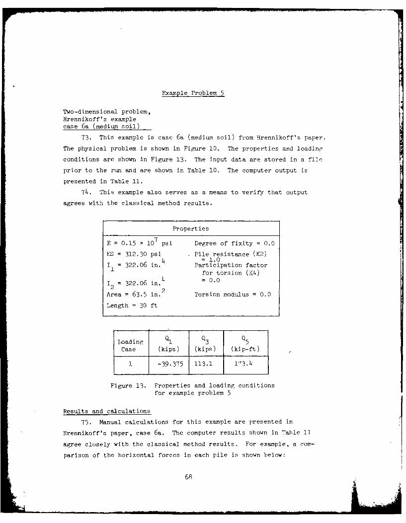
Example Problem 5

Two-dimensional problem,Hrennikoff's examplecase 6a (medium soil)

73. This example is case 6a (medium soil) from Hrennikoff's paper.

The physical problem is shown in Figure 10. The properties and loadinp

conditions are shown in Figure 13. The input data are stored in a file

prior to the run and are shown in Table 10. The computer output is

presented in Table 11.

74. This example also serves as a means to verify that output

agrees with the classical method results.

Properties

E = 0.15 x 107 psi Degree of fixity = 0.0

ES = 312.30 psi Pile resistance (W2)4 = 1.0I1 322.06 i~ .

1 Participation factorfor torsion (K4)

1 = 322.06 in.4 = 0.0

Area = 63.5 in. 2 Torsion modulus = 0.0

Length = 30 ft

Loading QI Q3 Q5

Case (kips) (kips) (kip-ft)

1 -39.375 113.1 173.4

Figure 13. Properties and loading conditions

for example problem 5


75. Manual calculations for this example are presented in

Hrennikoff's paper, case 6a. The computer results shown in Table 11

agree closely with the classical method results. For example, a com-

parison of the horizontal forces in each pile is shown below:

6P3

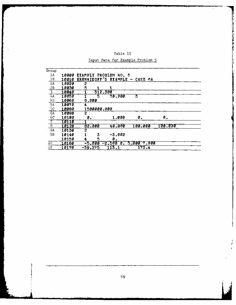
Table 10


Group1A 10000 EXAMPLE PROBLEM NO. 5B 10010 HRENNIKOFF'S EXAMPLE - CASE fA

2A 10020 22B 10030 5 1 13 10040 1 312.300hA 10050 1 5 30.000 3hD 10060 9.0005A 10070 45C 10080 1500000.0006A 10090 2

6c 10100 0. 1.000 0. 0.7 10110 1"8 10120 82.000 40.000 100.000 100.0309A 10130 29B 10140 1 3 -3.000

10150 4 5 0.10 10160 -5.000 -2.500 0. 3.000 7.00012 10170 -39.375 113.1 173.4

69

, . . . . . . . . . . . . . . . .. . . . . .. I .. .. .. .. -. . .. ' . . . . .. .. . I I I I I I I . . . .. . . .. .. . il j

Table 11


EXAMPLE PRObLTM .O. 5HRENNIrOFF9S 9XAMPLE - CASE 6A

NO. OF PILE ROWS - 5 P MATRIX IS CALCULATED FOR EACH ROW


PILE NUMBERS

1 5 r - 0.I5E 07 PSI IX = 312.09 IN**4 IT = 312.36 IN**4AREA = 61.6 IN**2 X 9.00 IN = 9.20 INLENGTH = 30.0 FEET ES = 312.300I1 - 0.4107 K2 - 1.0000 13 = 0.14 - 0. K5 - 0. K6 = 0.

ALLOWALrL : COMPRESSIVE LOAD = A2.00 KIPSTTNSILE LOAD - 40.000 KIPSVENDING - 6e.o00 KIPSMOMENT - 100.000 KIP-FT

TIE B MATRIX FOR PILES 1 THROUGH 5 IS

0.779E 04 0. 21.0. 0.265E Of 0.0. 0. 0.


PILE ROW BATTER U1 (?T)1 -3.30 -5.0002 -3.00 -2.5093 -3.00 0.4 VERTICAL 3.0005 VERTICAL 7.000

3. STIFNESS MATRIX S FOR TE STRUCTURE

0.1161 06 -0.132? 06 -0.695t P7-0.2321 06 0.125F 07 -0.1031 OP-0.g51 07 -0.1037 OR 0.320) 10

3A FLEXIBILITT MATRIX F FOR THE STRUCTURE

0.2057-04 0.4'7-05 0.5661-070.4?7E-05 0.1711-05 0.1441-076.5e61-07 0.l44!-oly @.48T-099

COORDINATES Of ELASTIC CENTERECI 0.003 EC, - [email protected]

(Continued)

70

Table 11 (Concluded)

LOADING CONDLT1OV I


Q1 03 95-39.375 113.100 173.400

5. STRUCTURE DEFLECTIONS (I4Cfl5

D1 D3 D5-0.237E 00 0.553r-01 0.3F8Y-93

6. PILE DEFLECTIONS kLON PILE AXIS (INCHES)

PILE Xl X3 X51 -0.172E 00 0.13cr 30 3.3058E-032 -0.175E 0 0.129F 00 0.3rBF-033 -0.179E 00 0.118F 00 0.3981-034 -0.207r, 00 0.420E-01 0.3681E-35 -0.207r 03 0.2431-01 0.36RE-33

7. PILE FORCES ALONG PILE AXIS (KIPS & FT)

PILE 71 73 75 FAILURVBU CO TI

1 -1.338 36.790 F.2 -1.165 34.014 0.3 -1.3)2 31.237 0.4 -1.611 11.137 0.5 -1.611 6.454 0.

TOTAL NO. PAILURES - 0 LOAD CASE I

8. PILE OCES ALONG STRUCTURE AXlS (I1S VER?

PILE 7I 7' 7"1 -I'.q0o 34.479 F.2 -12.051 31.836 F.

3 -11.199 29.194 0.4 -1.611 11.137 0.5 -I.1i 6.451 0.

SUM -3n.375 113.106 173.43?

• ' ~~ ~~i e ~~**veeeeo~eeo eooe~oeoeeeeoeo~e*

F (kips) from

Pile Computer Hrennikoff'sNo. Output Example

1 1.338 1.34

2 1.365 1.37

3 1.392 1.39

h 1.611 1.61

5 1.611 1.61

76. The vertical pile forces also agree closely and are shown

below:

F 3 (kips) from

Pile Computer Hrennikoff'sNo. Output Example

1 36.790 36.8

2 34.olh 34.o

3 31.237 31.2

4 11.137 11.1

7P

Example Problem 6

Two-dimensional prob-lem, 16 piles withlinearly varying soil moduli

77. To further illustrate the use of program LMVDPILE for two-

dimensional systems, a sixth example problem was run. The B-matrix

terms are input directly. The physical problem is shown in Figure 14.

The properties and loading conditions are shown in Figure 15. The input

data are stored in a file that is listed in Table 12. The computer out-

put is presented in Table 13.

78. This two-dimensional example was run to verify that the com-

puter results agree with the St. Louis District's program output.

6.o'8.e j8.0'. 8.0'6.0'.0' 8.0'. 8.0 8.0', 0 8.0' 8.0 8.0 8.0' 8.0'ORIGIN UUPf~ iilihPHFigure 14. Physical problem for example problem 6

Properties

b = 5.6 E = 30,000.0 psi

b 448.o KS = 0.001 pci22b = 0.001b1 = 0b31 0

Loading Q1 Q3 Q5

Case (kips) (kips) (kip-ft)1 -0.11 2.678 -177.5

2 -0.11 3.110 -206.67

3 -0.11 0.028 -1.233

Figure 15. Properties and loading condi-tions for example problem 6

73

Table 12


Group1A 1Z 020 iXANLL ?. JKEA NC. 61B 1v 1Z Jjii\ i C'i-RTON -C.C:, AND DC, JFiAME ADZAC.i';2A Ia.2e 22B 143U 1E, 13 12 42 0.001TA 1ZO50 1 ic 4Z.Z22 14B ia£6o 5.521 e 445 .c2-O z.ei Z.

5A 1e?7Z 45C 1 2 J020.0Z26A 1ZJ7 1

7 IZ1I£ 1

8 1Z12- Z.565 - . m3 0.1 ?.19A 10153 29B 1Z14e 1 2 -4 .a2

le1:2 3 16 2.

1Z170 I .,1 . 1 ,2 .

12 1z 16 -,.11Z 2.E7i -177.500I lz -.? .11@ 3.11? - - . 7

r Table 13Output Data for Example Problem 6

OVLRO& LJZ& AN.) ZAM1 SERA15 ADJACENT

NC. jr PILE ?LdS = It b MATFIX IS ZALCLLATED iJOS fiTSCi I1. An,! OF PIES. AND SOIL DATA

1561 e.321 AS PSI ts Z.01 2 L et1 .1.201z 0 .02I 2

ALLO.A.:.S% CLOIP , SIV. Loh) ?*DCL LIPSTENSILE LO AD , eSS SIP SBtNDING Z .122 IFPSmOMENtT 0.e~i .IP-FT

h ATFIX INPUT OIFATTL7 AND lIN. -CSIPIEO H5 tIIITIES

Td. . MAIRIS SOP PILE, 1 TARJOOA 15 15

2. Tk.Lz O)FPILE ZOOADINATIS AND BATTER

jiLt 60. BAITER i1 MI)

2 - 4.50 14:t5

0 VS.U11C iZ 22.52/4 AE , IiSkL V.bee

- VEnTIZAL 7- .5/2

7 AFT CAL 04.2- V.SSTICAL I ZSA

o 512A 705-to

11 VRI CAI 5.AP

14 Y,1IL ISPF/it iESRT;CSL 11I ,0I' V EnTI CA L I12.5.2

e.14c5 SI! -e.2SSi V. 7 -2F e5- e5, /0271: 1:- -71 1/7

e.250.25 -?.'l; e7 V .TC t I71

5A tLtVIiILiTE "ATE:A iFPR Tq! FDFOLTJII,

(Continued) (Fheeot, I of 7)

75

Table 13 (Continued)I

4. M41616 21 APPLIED LJAOS (KUS & T

01 03 0- . 2.67 -177.5.0

b. S!AJZTOSRE DA)LE0110N0 (INCHES)

D1 03 0)5-,4.244i 20 ?.361 i tO _?.I 02-04

F. PIL. DLFLECTIO.E ALDN; PILE AXIS (IKC41S)

PILL XI X3 4±1 -. 1460 60 2.410; U0 -0.10.51-24Z -. 14'OE 22 2.4111 O -e.1236-243 -8.244i 2e0 3.064 00 -0.123E-044 2.2446 2e ?.-6-; U0 -. :I0e0-Z4

A 22442 2! a.66 I0 -. 02:-

6 -02.244i it2 0.5676 0e -0. 1026-247 -4:244L ae Z.3661 0 -e0.1 03E-24§ -4 i44i ?.5666 20 -0.103i-24

-. 2 44. Z2, 2.27e: 00 -a.1031-24Ic -Z.2441 W0 I.071: 00 -2.1?51-2411 -2.2441 21 222,A 0.0,212 -22446 P2 Z.231 0 -. 0~1.0 -Z.244L Ve C.5746 20 -0.122>214

14 -2.244i W0 2.37% t -e0.13i1Z415 -2244, 2 e 0.761 00 -e.1031-2416 -2244i 22 e.3776 60 -e.122-14

. . .. . . . . . . . . . . ... . . .............. ... . . .


76

LOA

EA

Table 13 (Continued)

7. PILL FOCES ALr,&N PILE 6I1$ (KIPS S. F

PILE i1 13 isrILnEU CC L

1 -2.ZI .I 4 -r.00

. -2.21 P.1_4 -0.? aP_0.241 2.13 -02 F-?.e01 ?.14 -. 0 0 e P

6 -2.201 ?.164 -e.20 F

S -. -. .0 0 F-. 01 1.1 - -.00

16 -. CC 2.166 - -.211 - . 0. 1 6 -.~ -2.020 F1 -.1 2.67 -0.022 F

1.5 -2.21 2.1 6 -2. 2 0 F

14 -2.2 1 Sta, -3.01 P1D -Z.201 Z.163 -.0016 -2.121 P.162; -2.000 F

TCIAL- .4. PAILUE6ES 1t LOAD C551 1

.. . ............. .. . . . . ...... . . . . . . . . . . . . .

PI. FlPJACS ALONG ST&22?U01 AXIS (LIPS F;562)

1 -2.145 2.176 -e.00

-2.U (Shee1 3o0.0024 -a 13 -2.200

5 -0.021 2.164 -0.200-2e2 212 -. 00I

7 -2.61 .16! -220

-'.221 2.165t -0.012,

12 -1.01 2.112 -2.00eIc~~~ -2Ei t7 -0.eel

13 -2.101 2.117 -2.e00

1 1.5 z.1-6 -2.020

SUM -e.110 2.t724 -177.500


77

Table 13 (Continued)r

.EJALINE Z2N3IT13-. 2*~'*

..... ....... * ..... . .~....... . ....

1. "12912 Jr ,2PLIED .3932 ; (4112 FF1!,

-K12 3110 -221.117

...*.,*,.t........ *.

ZI 3. k 3 2

.- 14- e2 .43 2 -. 21-

1 -:.314'E-212.423, le -e.219o-2- 4.'3±-. 2e.42 iZ -2.219E-5 -2. Z3 2.431 22 -21 -5

4 -,. 1437 12k 2.43 , ,2 "-?t1

-2.43± e2 .43 2, 2 -0.21 t-2'.141 22 2.433; 22 0.1

72 -Z.114!i2

e1 Z.433- 22 -2.211OI-2.143E11: 2.4231 22 -Z.21JE

1 2.i1431 42 2.4339 22-22112 -I 12 2 .31 2 2 .29E-21 2 -143i 22 .434i 22 -e.219-214 -2e.1 43i 22 e.444-. 2 -2,11-2Z51: _0.143E 22 2. 4,41 22le 21±1, -2.143: 1. 434. 22 -2 .21 1-2

(Continued) (Sheet 4t of 7)

78


7. ?£I FL t r t I1 AO k ILPJ,

Zz 0- - rAIie

22£o 2.sicz -0.1e. F4 -. Z25 2.19- -1-.200 F

-. 101 t.14 -2.200 f

e 2.2 weI Z.1 94 -2.ei0 F0.2 e.194 -0.212Ze

1 2 1e.221 e.134 -Z .2 Fe

14 -2.201 e.13 -2 . 0&S-2.201 0.19 -2.I2

1-2 1 -.4o -22 F

GTINO. FAILURiS * IF £49 CASE Z

2. ItS )R0ZS ALONG S 0J TRuE AXIS (KIPS F-FI)

I IL Fl 13 F1 0' -2.24 2.7 -02002 -Z.249 2.13 7 -0.0e0

-2 :.22; 0.1;3 -0.0004 -. 1 .1e I- 3 -2ee0

-2z.22:i 2 .S' -2 .200e

- -2.e1I1 Z2.134 -2.22el-02 e .134 -2'.200

11 -201 2:1r4 -2.22211 ?~ - Z0 z.14 -2.2000

12 l -. 2 2.1-4 -0.220

13 -2.01 .4 -2.200

I tI -. 221 2.194 -0.0200

It -. e1 0.19t e0.000

sU Z2.I12 3.110 -- -- - -- - -- -- - -- - -- -- - -- -


79

Table 13 (Continued) I

~*LGAJIt.J o.%D:TION 3

4. MIATRIX Of APPLIED COADF (LIPS &d 1FI

(1 3-a.11t 2.Z28 -1.253

5. 67RJ2'TJS DtxI,.ZTIJNS (INCHEAS)

31 L53

bFILDDfLECTIONS ALON^T PILE AXIS (ItCHES

PILE X1 13 X51 88. eo 2.1356 E -t _ E.958S-4

36,6b it e.143; Le -0-51-:-04335 2 -t.16001 -A.e5S1E-24

3Z851 zt -A'.597X-A1 -. S58E-t04-Z3 5S it -Z.t15Lt1 -t.45 3L-i446O.95i 320.431 A -0 8.6-?4

7 z51 it -0.3506-e1 -0.358t-2

4395 A -0.2631-Al -O.E458!-04

359 it -t.135t-a1 -0 .3586-Z4

1-289S!F At -t .20?t -22: - 088-42-2.3953 Vt .A7t-t2 zta -038-4

13 -2.,S 21-5 Z 8 .1 44-Ae -2 . 356-414 -. 35ie 92 226E-tI -0 , 98-.41-0:,5 2, te2 0-1 -358F-04

I e -2 05 .2 t.31t-1 -8.581-04

(Continued) ( r

8o

FI


7.PILE FOCES ALON; PILL AXIS (1PS F1)

FR 2 5 iR FAILJKOrU CC 7Z

1 -2.205 0.061 :a.at02 -2:.105 _.64 -0.e03 -e.35 -a.e3e -0.o0i -. Z25 2.227 -e.200

5 -3.005 -. I0 2 -0.ee5 -. 005 -. 201-3 -0.007. -2.025 -Z201 -e.0201A -Z.205 -2.2 -6.00019 -220S -2.20 -0.00

12Z -2.002 -Z.20 -0.020

14 -2.25 0.010 - .015 -e.05 0 .214 -0.0016 -0.5 .13 -0.020

TOTAL No. FAILURES 0 LOAD CA Z

9. PILL i2J0~OS ALONG STA.JT200 3210 (L[PS 0007?

MEt F1 F3 F5

3 -2.05 -0.31 -0.000

.-,01.05 -2.010 -021 htoS -0.e05 0.23 -0.e0

7 -0.005 -0.023 -a.000'3 -a2.0l5 -2.015 -3 .tOO9 -0.00 -P.016- 3.0

10 -0.M05 -q.US -2.00211 -e.00 -79 e. -3.00012 -0.:205 2t3 -. 013i -0.00 2.006 -0.01014 -0.0Z05 2. 01 0 -.15 -3.005 12014 -0e30016 -2.005 a.1 -000

sumh -0.112 2.a29 -1.233

...... ... ......

ready

(Sheet 7 of 7)

81A


79. The computer results presented in Table 13 agree closely

with answers from St. Louis program output. For example, for pile 1 and

loading case 1, the pile forces along the structure axis from Table 13

are

F1 -o.05 kip

F = 0.178 kip3

F = 0.05

as compared with

F1 = -45.4 lb

F = 178.1 lb

F5 =0

from the St. Louis program. The results for all piles agroc very

closely.

• 82

Example Problem 7

Three-dimensionalproblem, 4 pinned pilesand constant soil modulus

80. This example problem illustrates the use of program LNVDPILE,

given four vertical piles (similar to example problem 1 for 2-D system).

Figures 16 and 17 show the physical problem. There are six loading

conditions: a unit load applied along each axis, a unit moment about

the U1 and U2 axes and a combination of all loads. Figure 18 shows the

loading conditions and properties. The input data are stored in a data

file prior to running the program and are shown in Table 14. The com-

puter output is presented in Table 15.

81. This example illustrates how a three-dimensional problem with

linearly varying soil modulus is coded. It also serves as a means to

verify the computer output by comparison with manual calculations.

A A

U2

Figure 16. Plan view of example problem 7

83

ORIGIN U

U3

Figure 17. Section A-A for

example problem 7

Properties

Ult. str. of concrete = 5000 psi Vertical (h = 0.0)

KS= 10.000 pci

I, = 833.333 in. 4 Degree of fixity = 0.0

12 = 833.333 in.4 Pile resistance (K2)0 in. 2 = 1.0

Area = 100.0 Participation factorfor torsion (K)= 0.0

Length = 100.0 ft Torsion modulus = 0.0

Loading Q Q Q3 Q4 Q5 Q6Case (kips) (kips) (kips) (k:; 't 'kip-ft) (kip-ft)

1 1.0 0.0 0.0 0.0 0.0 0.0

2 0.0 1.0 0.0 0.0 0.0 0.0

3 0.0 0.0 1.0 0.0 0.0 0.0

4 0.0 0.0 0.0 1.0 0.0 0.0

5 0.0 0.0 0.0 0.0 1.0 0.0

6 1.0 1.0 1.0 1.0 1.0 0.0

Figure 18. Properties and loading conditionsfor example problem 7

84

Table 14Input Data for Example Problem 7

Group1A 100OZ EXAMLT FROSLEM %0. 71B 1ee12 IFETICAL Mrs &ITH UNIT 10 ____________

l.A 20~2 1 4 1@0 .004. 2 _______

4.C jog6k e33.33Z! P33.333 100 .. 00 10.000 le.oze IPILE GEzammy5A 1e?2 1 _______

5B 110S 0.2 ~.o ~L 4TRA9A INN ________

6c 10122 e. 1.e00 0. e. IPILE PUXITUEST 10110 13000 1 -e. ez lee..c lee.ee 1.30.4e 120.2/ imp.e i~..M UO

§' '10 1.04 0. a. 2.r 2.Am otzcrfo9B1125 . 1002 10. 1 .if CORDN.E

10210 0. 0. 2. 1.910e 0. e.U226~ 0. 0. 0. 0. 1.200 ?.1023e i.et~o 1.C00 1.00a 1.2 1.Pe0 2.

85

Table 15


IAMNL PROBLEM NO. L

IETICAL PILIS WITH UNIT LOADS

N. OF PILES - 4 B MATRIX IS CALCULATED FOR EACH PILE


FILE NUMBERS

1 1 - 0.43! 07 PSI IX = 83n.33 IN**4 IT = 833.33 IN**4AREA -168.0 IN**2 X 10.68 IN T . 10.66 INLENGTH = 100.0 FEET ES - 10.000E1 - 0.4107 [2 - 1.0060 K3 - 0.E4 = 0. [5 - 6. [6 - 0.

ALLOWABLES: COMBINED BENDING YOR TENSION - 100.00 KIPSMOMENT ABOUT MINOR AXIS FOR TENSION - 109.000 lIP-FTMOMENT ABOUT MAJOR AXIS FOR TENSION - 1 ,.680 lIP-FTCOMBINED BENDING FOR COMPRESSION - 100.060 KIPSMOMENT ABOUT MINOR AXIS FOR COMPRESSION = 1 16.008 lIP-FTMOMENT ABOUT MAJOR AXIS FOR COMPRESSION - 186.086 KIP-PTCOMPRFSSITE LOAD = 160.000 KIPSTENSILE LOAD - 160.060 KIPS

THE B MATRIE FOR PILES 1 THROUGH 4 IS

0.108E 85 8. 6. 0. S. 6.0. 0.18E 05 0. 8. e. 0.6. 8. 0.3571 06 0. 0. 0.0. 0. 0. 6. 6. 8.6. 6. 6. 6. 6. 6.0. 6. 6. 0. 0. 0.


PILE NO. BATTER ANGLE UI(PT) U2(FT) US(FT)I VERTICAL 6. 1.696 1.066 9.2 VERTICAL S. 1.000 -1.606 0.3 VERTICAL 9. -1.000 -1.900 0.4 VERTICAL 6. -1.009 1.600 0.


8.4332 e5 0. 8. 8. 6. 8.6. 9.4331 85 9. 6. 6. 6.0. 8. 0.143E 07 0. P. 6.

I. . 6. 0.206V 89 0. 6.0. 8. 6. 0.206T 09 6.

. . 0. 0. 6. 6.12Sf z8

3A FLEEIBILITT MATRIX F FOR THE STRUCTURE

0.2312-94 8. 0. 6. 8. 8.8. 0.231f44 0. 0. 0. .8. 0. 0.796E-06 6. 0. 8.6. 8. 0. 8.486t-08 F. 0.0. 6. 0. 0. 0.4869-06 0.6. 6. 6. 6. . 9.801E-07

(Continued) (, nr 7)

86


****** LOADING CONDITION I "0000"

4. MATRIX OF APPLIED LOADS Q (ZIPS & PPET)

QI Q2 Q3 Q4 Q5 Q61.000 0. 0. 0. 0. 0.


DI D2 D3 D4 D5 D60.231E-01 0. 0. 0. 0. 0.


PILE X1 X2 X3 14 I5 161 0.2319-01 0. 0. 0. 0. 0.2 0.2311-01 0. 0. 0. 0. 0.3 6.231F-01 0. 0. 0. 0. 0.4 0.2311-01 0. 0. 0. 0. 0.

7. PILE FORCES ALONG PILE AXIS (ZIPS & FEET)

PILE F1 P2 F3 P4 F5 F6 CBFTR FAILURECP IJ CO TE

1 0.250 0. 0. 0. 0. 0. 0.2 0.250 0. 0. 0. 0. 0. 0.3 0.250 0. 0. 0. 0. 0. 0.4 0.250 0. 0. 0. 0. 0. 0.


8. PILE FORCES ALONG STRUCTURE AXIS (ZIPS A FET)

PILE Fl F2 r3 F4 V5 F61 0.250 0. 0. 0. 0. 0.2 0.250 0. 0. 0. 0. 0.3 0.250 0. 0. a. 0. 0.4 0.250 0. 0. 0. B. 0.

SOD 1.UOe 0. 6. 0. 6. 0.00

(Continued) (:hcet 0" 7)

87

rI


A***** LOADING CONDITION 2 ****

4. MATRIX O APPLIED LOADS Q (TIPS & 111T?

Q1 Q2 Q3 Q4 Q60. 1.006 0. 0. o. 0.

5. STRUCTURE DFLECTIONS (INCBHS)

Dl D2 D3 D4 D5 D60. 0.2311-01 0. 0. 0. 0.

*.*.*..*........**..*e......*****************..********

6. PILE DEFLICTIONS ALONG PILE AXIS (INCRIS)

PILE 11 12 13 14 15 161 0. 0.2311-01 0. 6. 0. 0.2 0. 0.231E-61 0. 0. 0. 0.3 0. 0.2312-01 0. 6. 6. 0.4 0. 0.231K-01 0. 0. 1. 0.

7. PILE FORCIS ALONG PILE AXIS (KIPS & PET)

PILE Fl F2 P3 14 P5 F6 CBFTR FAILURECD RiJ CO TX

1 0. 9.250 0. 0. 0. 0. 0.2 0. 0.250 S. 0. 0. 0. 0.3 0. 0.250 0. 0. 0. 0. 0.4 0. 0.250 0. 0. 0. 0. 0.

TOTAL NO. PAILURIS - 0 LOAD CASE 2

S. PILE FORCES ALONG STRUCTURE AXIS (ZIPS & ?PIT)

PILE F1 2 P3 F4 F5 P61 0. 0.250 0. 0. 0. 0.2 6. 0.250 0. 0. 0. #.3 6. 0.250 0. 0. 0. 0.4 0. 0.250 0. 0. 0. 0.

SUm 0. 1.000 0. 0. 0. 0.000

(Continued) (Sheet no 7)

(Sheet oC-7


****,** LOADING CONDITION 3 *****

4. MATRIX OF APPLIED LOADS Q (ZIPS & FEET)

Q1 Q2 Q3 Q4 Q5 Q6.i.e o. 1..

5. STRUCTURE DIFLECTIONS (INCHES)

DI D2 D3 D4 D5 D60 • . 0.7001-03 0. 0. 0.

S. PILE DEFLECTIONS ALONG PILE AXIS (INCHES)

PILE 1 X2 X3 X4 X5 X6

1 0. a. 0.78111-03 0. 0. 0.2 41. 0. 0.7001-03 6. 0. 0.3 0. 0. 0.760-43 0. 0. 0.

4 9. 0. .7301-03 0. 0. 0.

7. PILE FORCES ALONG PILE AXIS (KIPS & FEET)

PILE 11 P2 P3 F4 F5 F6 CBFTR FAILURECP BU CO TE

1 0. a. 0.250 Q. 0. 0. 0.002 0. 0. 0.259 0. 0. 0. 0.003 0. 6. 0.250 0. 0. 0. 0.004 0. 0. 0.250 S. 0. 0. 0.00


S. PILE FORCES ALONG STECtURE AXIS (KIPS & FiT]

PILE P1 72 P3 P4 P5 F61 0. 0. 0.250 0. 0. 0.2 0. 0. 0 .250 0. .3 0. 9. 0.250 S. 0. 0.4 0. 0. 0.250 0. 6. 0.

SU" 0. 0. 1.000 -6.000 -0.000 0.

(Continued) (Sheet o' 7)

89


*SS***S* LOADING CONDITION 4 *******

4. MATRiX OF APPLIED LOADS Q (KIPS & FEET)

Qi Q2 Q3 Q4 QE Q60. 0. 0. 1.000 0. e.


D1 D2 D3 D4 D5 DE0. 0. 0. 0.583E-04 0. 0.


PILE X1 X2 X3 X4 X5 Xf1 0. 0. -. 7001E-03 0.583:-e4 0. 0.

3 0. 0. -0.700E-03 0.583E-04 0. 0.4 0. 0. 0.70E-03 0.583E-04 0. 0.


PILE F1 F2 F3 F4 F5 Fe CBFTR FAILURF

CP B CO TV1 0. 0. 0.250 0. 0. 0. 0.002 0. 0. -0.250 0. 0. 0. 0.003 0. 0. -0.250 0. 0. 0. 0.004 0. 0. 0.250 0. 0. 0. 0.00

TOTAL NO. FAILURES = 0 LOAD CASE 4

a.***********..s**sf******************************************** *

8. PILE FORCES ALONG STRUCTURE AXIS (KIPS & FEET)

PILE F1 F2 F3 F4 F5 F61 9. 0. 0.250 0. 0. 0.2 0. 0. -0.250 0. 0. 0.3 0. 0. -0.250 0. 0. 0.4 0. 0. 0.250 0. 0. 0.

SUm 0. 0. -0.000 1.000 -0.000 0.

es..n**..***** *.*fl--inflfl--gflinenn*** ***** .*******

(Continued) of

no


* LOADING CONDITION 5 *

4. MATRIX OF APPLIED LOADS Q (KIPS & FEET)

Q1 Q2 Q3 Q4 Q60. 0. 0, 0. 1.000 0.


D1 D2 D3 D4 D5 D60. 0. 0. 0. 0.583E-04 0.


PILE XI X2 X3 X4 X1 X61 0. 0. -0.700E-03 0. 0.583E-04 0.2 0. 0. -0.700E-03 0. 0.583E-e4 0.3 0. 0. 0.700E-03 0. 0.583E-04 0.4 0. 0. 0.700E-03 0. 0.583E-04 0.

7. PILE FORCES ALONG PILE AXIS (EIPS & FEET)

PILE F1 F2 F3 F4 F5 Fe CBFTR FAILURE0 CB BU CO TE

1 0. 0. -0.250 0. 0. 0. 0.002 0. 0. -0.250 0. 0. 0. 0.003 0. 0. 0.250 0. 0. V. 0.004 0. 0. 0.250 0. 0. 0. 0.00

TOTAL NO. FAILURES = 0 LOAD CASE 5

8. PILE FORCES ALONG STRUCTURE AXIS (KIPS & FERT)

PILE F1 F2 73 P4 F5 Fe1 0. 0. -0.250 0. 0. 0.? 0. 0. -0.250 0. 0. 0.3 0. 1. 0.250 0. 0. e.4 0. 0. 0,250 0. e. 0.

SuM 0. 0. -0.000 -0.000 1.000 0.

(Continued)

7 AD-AGA 191 ARMY ENGINEER WATERWAYS EXPERIMENT.STATION

VICKSBURG MS F/6 13/13DOCUMENTATION FOR LMVDPILE PROGRAM. (U)JUN 80 D K MARTIN, H W JONES. N RADHAKRISHNAN

UNCLASSIFIED wES-TR-K-A0-3 NL

I3f IIIIIIII

EIIIIIIIIIIIIlEIIIIEEEEEEEIIIEEEEIEEEEIIEIIIIIIIIIIIIIIIEEEEEIIIEII


4. MATRII OP APPLIED LOADS Q (lIPS & FEET)

Qi Q2 Q3 (4 Q5 Q6

1.980 1.60. 1.90 1.006 1.090 0.


"DI D2 D3 D4 D5 D60.2311-01 0.2311-01 0.7001-03 0.5832-04 0.583F-04 0.


PILE 31 X2 13 X4 X5 36

1 0.2313-01 0.231Z-01 0.7001-03 0.583t-04 0.5831-94 0.

2 9.231t-01 0.231E-01 -0.T169-03 6.583E-04 0.5831-04 8.3 0.231S-f1 0.2311-01 0.780.-03 0.583E-04 0.5833-04 6.4 6.2313-01 0.2311-01 0.2101-02 0.5839-04 8.5831-04 0.


PILE F1 F2 F3 P4 F5 F6 CBFTR FAILUROCS BU CO TE

1 6.250 0.210 6.250 0. 0. 0. 0.02 0.250 0.250 -0.250 0. 0. 0. 6.0.3 0.250 0.250 6.250 0. a. 6. 6.004 6.250 6.250 0.750 9. 0. 6. 0.01


8. PILE FORCES ALONG STIUCTURE AXIS (KIPS & FET)

PILE Fl 12 73 14 F5 101 0.250 0.250 0.250 0. 6. 6.2 0.250 0.250 -6.256 6. 6. 6.

3 0.250 0.250 0.250 9. 6. 6.4 0.250 0.250 0.750 6. 0. 6.

SUm 1.666 1.669 1.686 1.60 1.006 0.066

(Sheet 7 of 7)

92


82. The pile forces can be calculated by satisfying equilibrium

EF = 0 . These were found to agree with the program output shown in

Table 15. For example, in loading case 3 with a 1-kip vertical load,

the force in each pile is 0.25 kip. The force on each pile is

FH = 1/4 (applied vertical load) = 1/4 (1 kip) = 0.25 kip

The displacement in each pile is equal to

1PL _ 1 × 100 X 12 103- = 0.7Xl0 in.

AE 4300 x 144 x 100

This result also agrees with the computer program results.

83. In loading case 4, a 1 kip-ft moment is applied about the

U -axis. The pile forces can be calculated by satisfying equilibriumMu, =0 .

%1

EMu 1 F31U1 (1) - F32U1 (2) - F33U1 (2) + F34U1 (l) +Q4

where

F3 = vertical force in pile n, n = 1 - 4n

Q4 = applied moment = 1 kip-ft

UI = horizontal distance along the Ul -axis

U1 (1) = 1.0 ft

U1 (2) = 1.0 ft

:.EMu, = F31 - F32 - F33 + F34 + 1.0 = 0

From symmetry F31 = F34 and F32 F33

:.1F3nI = 0.25 kip

93

This result agrees with the computer output.

84. Load case 6 can be obtained as a superposition of load cases

1 through 5. The deflections of the piles and the load on each pile

can also be obtained by superimposing the respective results for load

cases 1 through 5. The following computations verify the computer

results in item 6 (deflections) and item 8 (loads).

Deflect ions

Pile Load X1 X2 X3 X4 X5No. Case (in.) (in.) (in.) (rad) (rad)

1 1 0.0231 0. 0. 0. 0.2 0. 0.0231 0. 0. 0.3 0. 0. 0.7 x 10-3 0. 0.4 0. 0. 0.7 x 10_ 0.583 x 10- 0.5 0. 0. -0.7 x 10 0. 0.583 x 10-

6 0.0231 0.0231 0.7 x 10-3 0.583 x 10 - 4 0.583 x 10 - 4

2 1 0.0231 0. 0. 0. 0.2 0. 0.0231 0. 0. 0.3 0. 0. 0.7 x 10-

3 0. -4 0.4 0. 0. -0.7 x 10-3 0.583 x 10 0.5 0. 0. -0.7 x 10 0. 0.583 x 10-

6 0.0231 0.0231 -0.7 x 10- 3 0.583 x i0 - 4 0.583 x 10 - 4

3 1 0.0231 0. 0. 0. 0.2 0. 0.0231 0. O. 0.3 0. 0. 0.7 X 10 - 3 0. O.4 0. 0. -0.7 x 103 0.583 x 10 0.5 0. 0. 0.7 x 10 0. 0.583 x 10-

3 4 -46 0.0231 0.0231 0.7 x 10- 0.583 x 10- 0.583 x 10-

1 0.0231 0. 0. 0. 0.2 0. 0.0231 0. 0. 0.3 0. 0. 0.7 x 10 3 0. 04 0. 0. 0.7 x 10- 0.583 x 10 0.5 0. 0. 0.7 x 10 0. 0.583 x 10 - 4

6 0.0232 0.0231 0.21 x 10- 2 0.583 x 10- 4 0.583 x 10- 4

(Continued)

94

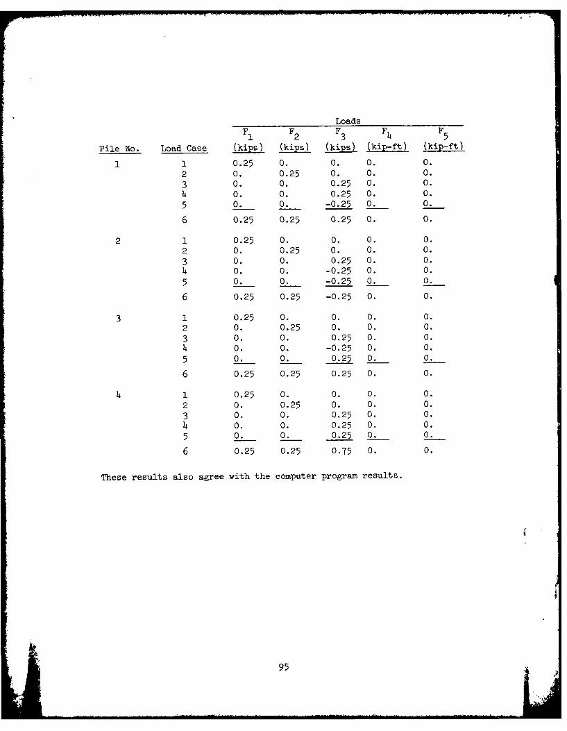
LoadsF1 F2 F3 F4 F5

Pile No. Load Case (kips) (kips) (kips) (kip-ft) (kip-ft)

1 1 0.25 0. 0. 0. 0.2 0. 0.25 0. 0. 0.3 0. 0. 0.25 0. 0.4 0. 0. 0.25 0. 0.5 0. 0. -0.25 0. 0.

6 0.25 0.25 0.25 0. 0.

2 1 0.25 0. 0. 0. 0.2 0. 0.25 0. 0. 0.3 0. 0. 0.25 0. 0.4 0. 0. -0.25 0. 0.

5 0. 0. -0.25 0. 0.

6 0.25 0.25 -0.25 0. 0.

1 0.25 0. 0. 0. 0.2 0. 0.25 0. 0. 0.

3 0. 0. 0.25 0. 0.4 0. 0. -0.25 0. 0.5 0. 0. 0.25 0. 0.

6 0.25 0.25 0.25 0. 0.

4 1 0.25 0. 0. 0. 0.2 0. 0.25 0. 0. 0.3 0. 0. 0.25 0. 0.4 0. 0. 0.25 0. 0.

5 0. 0. 0.25 0. 0.

6 0.25 0.25 0.75 0. 0.

These results also agree with the computer program results.

95

Example Problem 8

Three-dimensional prob-lem, 1 fixed vertical pile

85. This example problem has only one vertical pile completely

fixed into the rigid cap. It is similar to example 2 except the analy-

sis now is three-dimensional. Figure 19 shows the physical problem. A

1 kip-ft moment is applied about the U1 , U2 , and U3 axes. Figure 20

shows the loading conditions and properties. The input data are stored

in a file prior to running the program and are presented in Table 16.

The computer output is presented in Table 17.


by comparison with manual calculations.

U1

U2

Figure 19. Plan view forexample problem 8


87. In this example, 1 kip-ft moments about the Ul, U2 , and U3

axes were applied at the center of the structure where the pile is

located. The pile is completely fixed into the rigid cap. Therefore,

the resulting moments about the U1 , U2, and U axes are 1 kip-ft. These2 j 3

results agree with the program output presented in Table 17.

96

Properties

Ult. str. of concrete = 5000 psi K1 = 1.0756

KS = 10.000 pci K2 = 1.0

I, = 833.333 in. K3 = 1.4988

12 = 833.333 in.2 K4 = 1.000

Area = 100.0 in. K5 = 0.9990

Length = 100.0 ft K6 = 0.9990

Vertical = (h = 0.0)

Loading Q1 I Q2 Q3 Q4 Q5 Q6Case (kipE', (kips) (kips) (kip-ft) (kip-ft) (kip-ft)

0.0 0.0 0.0 1.0 1.0 1.0

Fig re 20. Properties and loading conditions for example problem 8

97

Table 16


Group1A 1Z0ZO 1XAFLE PRJL£I NO.IB 101J DNi FIXED VERTINAL PILE iIT.-. JNIT MOMENTS APLIED2A 1Me2O 32B 10030 1 1 13 10040 2 10.000iA 12062 1 1 l030.zeo 2-4C 10060 833.333 33.333 100.0i0 ii.000 10.0005A 10Z70 15B Ize0 5200.0ee 150.0006A Ioee 16B 1e100 1.00 I.076 1.0e 1.4938 1.ZZ 0.999 2.997 1Z110 140. .I0 .@1O 1Z@ .00 . 1o . 1• 10 o .8A 1120 z

10 1 130 0. . Z. ..11 114Z 0. Z. ..1.00 .20 1.zeo

readi

98

Table 17


EXAMPLE PROBLEM 0. 1ONE FIXED VERTICAL PILL IT11 UNIT MOMENTS APPLIED

NO. OP PILES 1 B MATRIX IS CALCULATED F3R EACH PILE


PILL NUMBERS

1 1 - 0.4"i a? PSI IX - 333.Z3 I.*4 I = 323.33 IN8 4AREA = 100.0 IN*'2 I - 10.00 IN T 12.00 INLENGTI 7 103.0 FEET ES - 10.04eX, = 1.0756 K2 - 1.0C00 £3 = 1.499eK4 - 1.2000 L5 z .2990e .6 e .SPF

ALLJ&ABLES: COMBINED BENDIN, FOR TENSION 10C.090 61SMOMENT "MOUT MIOR AXIS POE T ,SIDN = 100.?0 KIP-TMOM1NT ABOUT MAJOR AXIS FOE TENSION = 100.00e KIP-FTCOMBINED BENDING FOB COMPRESSION - 170.000 rI?S

MOMENT ABOUT MINOR AXIS FOE COMPRESSION = 100.700 HIP-FTOMINT ABOUT MAJOR AXIS ?OR OMPRESSION - 100.Z0 IP-FT

COXPOESSIV. LOAD - 10.00 KIPSTENSILE LOAD - 100.000 LIPS

THE B MATRIX FOR PILES 1 THROUGH I IS

e.US4L AS 0. e. Z. 0.131 27 e.0. 0.234L a5 0. -0.135X .7 0. e.Z. 0. 0.3!7E Ut 0. 0. Z.0. -e.13!E 77 C. Z.104i 06 0. ?.0.15E 07 e. 0. U. 2.124R e.U. U. e. 0. 0. e.100U 04

2. TABLE OF PILE 2OORDINATES AND RATTER

PILE NO. BATTER AN;LE JI(MT) U2(FT) 13FT)1 VERTICAL ?. 2. . U.

3, SIIFFESS MATRIX S IDA TAR STRUZTIUR

0.234E J5 2. P. 0. 0.13tB 07 0.Z. Z.2341 05 0. -?.135F 27 e. 7,

2. -.. 15 0?De. 0~e . 0.

0.2ZS 7 9. 0. 0. 2.124 9 e.0. 0. 7. 0. e. 7.IQ2F 04

3A iLEXIILITY PATRI I FOR THE STRJCTURF

0.925i-24 Z. e. 0. -o.12e5-z5 F.

. e2. r-Ui 0. a.120S-O 2.e. Z. 7.00-05 0. k. e.U. 7.DeE-05 U. 0.USUE-37 F. 2

* (Continued)

99


SLOAD11, CO1.D1T131. 1I

4. MAraIl OF APPLIED L3ADS 2 (SIPS & FEET)

a. a. a. 1.000 1.0ee 1.z30

5. SIBRITJRE DEFLICTIONS (INCHES)

DI D2 D3 DI Dt DO-L.144L-J1 t.1%4L0 0. 3.392E-23 e.302E-03 8.1205 Z2

C. PILE DEILL2TIOUS ALON PILL AXIS (INlaS

PILE 11 12 13 X4 15 X51 -9.144L-1 e.144i-01 0. 2.302t-03 8.3e26-03 e.12t 32

7. PILE PORCES ALONG PILL AXIS (KIPS S FLIT)

PILL F1 12 P2 P4 F5 F6 21714 FAILJR!CZ BU 23 Ti

1 0.800 -0.000 8. 1.000 1.000 1.000 8.Z2

TOTAL N3. PAILURiS - a L3AD CASE 1

6. PILL FOCKS ALONG STRUCTURE AiIS (KIPS & TE)

PILE F1 F2 F3 F4 P5 Fe1 0.90C -2.086 0. 1.818 1.eee 1.0ee

Sim 0.ree -8 v r. 1.080 I.Bee I 010

100

Example Problem 9

Three-dimensionalproblem, 27 pileswith constant soil modulus

88. To demonstrate further the use of program LMVDPILE an example

problem with a constant soil modulus is given. Figure 21 shows the

physical problem for this example. The properties and loading condi-

tions are presented in Figure 22. The input data are input interactively

and are shown in Table 18. These data are saved in a file and are listed

in Table 19. The computer output is presented in Table 20.

89. This example illustrates the option of inputting data inter-

actively for a three-dimensional problem with 27 piles (vertical and

battered) and a constant soil modulus. It also shows how the batter

can be input in groups.

O R I G I N - - ,

12I 9

in

in

3*5' 2.0' 4.0 2.0 2.0' 2.0'12 0' 2.0 ' 2.0' j2 O -I I 2 0i2.0 1-.5

35.0'

NOTE: PILINGS NUMBERED 1-12 ROTATEAT 270 IN DIRECTION SHOWN.

PILINGS NUMBERED 13-24 ROTATEAT 90* IN DIRECTION SHOWN.

Figure 21. Physical problem for exampleproblem 9

101

Properties

Ult. str. of concrete = 5000 psi K = 0.4107

ES = 200.0 psi K2 1.0

I, = 1728.0 in. DF = 0.0 K3-K 6 = 0.0

I = 1728.0 in. PR = 1.02 .2

Area = 144.0 in. PFT = 0.0

Length = 70.0 ft G = 0.0

Loading QI Q2 Q3 Q4 Q5 Q6Case (kips) (kips) (kips) (kip-ft) (kip-ft) (kip-ft)

1 0.0 276.961 3h4.9 5287.422 0.0 0.0

Figure 22. Properties and loading conditions forexample problem 9


90. The program output is shown in Table 20. From statics,

EF = 0 .

EF1 = Ql

where

F1 = horizontal pile forces along the structure axis (kips)

% = applied horizontal load in the U1 direction (kips)

EF1 = 8(-0.015) + 4(o.006) + 4(o.o8) + 8(0.018) + 3(-0.0011) = 0

Similarly

1F2 = Q2

Table 18

Interactively Input Data for Example Problem 9

INPUT DATA FILE NAVY IN AFRAU% OR LO._ FM ACARRIAOE RFTrAN IC MINPUT8DATA C!LL CON M3? UINA;L.

I NPUT A FILE NA' MBF DATA. I T CAR AVO --'h:IF TOOU D C NOT sANT To SAVE DATA FILE.

2 DEBT

INPUT TtC LINES OF PRCJ:EC? IDENTIFICATION NOT10 EXCTED CE ChAPACTEFS EACH

INFO' FIRST LIA'? EXAMPLr PACELEm NO. 9

INPUT SlMOND .Ip.r2 NC: ROA-PLV pMORLO'7 - -C:; A.7 :C j

DO TOO WANT TO RUN A 2-C OR 3-D ANAL'?1U2ENTCIR 2 OR 3 2 3

INPUT NUMBER OF PIL'S, PIE TRFOOPS, AN: oZ It:v IC'2 27,1,1

INPUT SOIL P;AOPOAT2 CATA - 4V A4t -F:ME-S=CN4STkNT $CIL OR -7J2=t1NTAPLT EAPOIA, OCILFS=SCBRADT MODULUS (PSI IF MU-i OR PCI I-- M'D2

? S,2et.A

DATA FOE PILE GROUP 40. - I

INPUT PILE SFAPO DTA:NPAIlD'NTIFICATIOE NUMBER OF FIpr PIL' IN GRDUPAPR-IDANTI2-ICATIDN NUMBER OF LAST PILE IN GROUPSLAN LENOTH OF PILE (FEET)NFS-COCE FOP TTPE OF INPUT To COMPUT' ELASTIC FILE CON'T, TO

S=INPUE PILE B MATRIX TERMS DIREZTLT2-ANT SHAPE PILE3- ROUND PILA

2 1.27.7t .P,2

INPUT AIX & AIT-MCMRNTO OF K'I N*Afr'A - CEOSS SECTIONAL N'R(I" *2U & Y - PILO DIMENSIONS ALUM" C T AX' - 's

? 1726.2.lO7t.144.i.I2.F,.12.FI

INPUT PILC MATERIAL DATA-MP (I-CONCp':. LTBT. I 'S:CIAL)7 1

INPUT US-ULTIMATE STR'AOTR OP ZCECR'TE PsEJWEWIGRT OF CONCRETE (PCE)

INPUT FIXITT DATA - NE (1-INPUT ALL FlOUTY ZOIEEICIANTSOR 2=INPUT DEUR'! CF FIXITY

?2

INPUT DF - DEGREE OF FIXITY 20.,11

PP - PlC' A'OSISTAC'r (I=?-A'A4 O UP' F1 ?PET - PAFFICIPATICN FACTOP EON TORSIONG TORSION MCDULUS (PSI)

(Continued)

THIS PAGE IS ;ylYI&4AL


INPUI ALLONABLE LOADS AND MOMENTS:ACBT=ALLOIALF AXIAL LOAD USED IN CO'AIBNED P,:2ND

FOR PILE IN TENSION (KIPS)

AMINT;ALLO4AALF MOMENT ABOUT MINOR PRINCIPIE X:FOP PILE IN TENSION (EIP-PT)

AMAJT-ALLOAArLE MOM'NT ABOUT MAJOR P-2NCIFL- AXIS

FOR PILF IN TENSION (EIP-?T)AUBCALLO.ABLE AXIAL LOAD USED IN COMBINED PENDIND

FOR PILE IN COMPRESSION (KIPS)AMINO-ALLOWABL

r MOMENT ABOUT MINOR PRINCIPLE 0X1

FOB PILE IN COMPRESSION (KIP-FT)AMAJC-ALLOWABLF MOMENT ABOUT MAJOR PRINCIPL' AXIS

FOR PILE IN COMPRESSION (I1-5T)ACL-ALLOWEBLT CMPRSSSIVE LOAD (KIPS)ATL-ALLO#ABLE TENSILE LOAD (NIPS)

2 OFJ.tlAe.,1eA .e,1F(..e.1 . . . .: F,.,t,.

INPUI IA: P=INPUT BITTER FOR EACh PIL; o

TAB NUMBT

CF SUP3ROUPS 1ICR TEE S ,E ?ETEF23

INPUT NFP-NO. OF FIRST PILE NLP-NC. OF LAST PIL'BATT-BAITR=BATT VERTICAL ON I -OPIZOAZALANGL=CLOCKWISV ANGLE BTI'F% POSITIVE X-AXIS OF I.

SCRUCIURE AND I-AXIS (DIRECTION )F BAITER) OF PILE DE;)

FOR PILE SUBGROUP - 1 ? 1,12,3,27e

FOR PILE SUBGROUP - 2 ? 13.24,3,90

FOR PILE SUBGROUP - 3 2 2t.27.1.9

ISIS PROGRAM GENERATES TH? EOLLOdING TABLIS:

TABLE NO. CCONTTTS1 FILE 1'4D SOIL DATA2 PIL COORDINATES AN; BATTER

STIFENVSS AND FLEXILILIIY MAT'IIS FE T-SCRUCTUP! AND COORDINATPS OF ELASTIZ CFTS

4 APPLIED LOADSSTRICTURE DTPLECTIONO

6 PILE DEFLVCIIONE ALONG PILE AXIS7 PILE FORCES ALONG PILET AXIS8 PILE FORCES ALONS STRUCTURE AXIS

INPUT TBr

NUMBERS 0 TEE TABLES FOR HHICR TOU ANT THE OUTPUt.SEPARATE TB! NUMBERb dIfT COMMAS. ? 1,2,3.4.5. .7,B

INPUT A FILENAME FOR TABLE A IN A CHARACTERS OR LESSIF TOU *ANT TO 30 T!IS INFORMATION FCX A Nh RU..ill A CARRIAGA R

TPN IF YOU D NO7 a.N. TIS tiF.

INPUT A FILE NAM- FOR OUTPUT IN A CH4rACTEPS OR L'OS.BIT A CARIAG' lETUEN IF OUTPUT IS T PPINTFD ON T ':RA:.

INPUT US'S - DISTANCES FOR ORIGIN TO PIL'ALONG UX 4xis

V 14.DE,6.2,-2.-6.-Sd.-14.I2.4.-4.-2.2.r.-4.-12.14.I ...

INPUT U2'S - DISTANCES FROM ChlI 0O PILr

ALONG U2 AXIE

INPUT UW'S - DISTANCES FROM OBIIl1 TO ILEALONG U3 AXIS

? 27*0.0

INPUT APPLIED LOADS AND MOMTNTS:Q1 & Q2 - HOPIZONTAL LOADS ALONE Ul £ U2 NXiS (KIPS)

03 - VERTICAL LCAD ALONG U3 AXIS NKIPS)Q4,5,.Q - MOM'NTS ABOUT UI,U2,U3 AXS (EIP-FT)

F0 LOLLING CONDITION - 1 ? 0.? ?9.r 11 4.'- 7:.. r.

i04

THIS ?A Z IS RiST 7U11 T7 A,1CQJ3L-

, ei r

L '7..

Table 19


Group1A 10002 EXAMPLF PROBLEY NO. 91B 10010 NOD EXAMPLr PROBLEM - CONSTANT SOIL MODULUS2A 10020 32B 1030 27 1 13 10040 1 240.00ehA 10050 1 27 70.1M 2hc 10060 1728.00e 172.020 144.20 12.300 12.2225A 10167. 15B 1082 5000.e22 15e.006A 1e096 26c Ie10o 2. 1 .20e 2. 2.7 12112 1022 .oe 1922.1 1200 .22 1i22 q 1,,ov mo0 imoz -m im mk un .78A 1012e 0

101U2 'K22 27e.2 14.22 1.5-, Z.10 12140 3.ZZ 27e.ke 1.eo 1.52 2.

10156A 3.22 27a.e 6ea 1.52 2.1I16e 3.22 270.,60 2.e2 1.50 e.1017e 3.2Z 270.90 -2.02 1.5? e.1e180 Z.eO 270.00 -6.20 1.50 0.12192 3.ZZ 272.e2 -i.22 1.52 e.10200 32.0 272.22 -14.00 1.52 2.10210 3.e0 27e.00 12.00 4.52 2.1022 3.@e 272.Z2 4.Z2 4.5t 0.1623e 3.2Z 270.S2 -4.00 4.EC 2.10242 3.00 270.2Z -12.60 4.52 2.10250 3.22 92.to 12.00 .,6e e.12260 3.00 90.02 e .2 9.:.7 Z.1027e 3.zic 92.22 -4.22 L.2 e.1028 3.20 90.00 -12.20 ..0 2.12292 3.z0 9?.22 14.02 12.e 0.12322 3.2z 92.ce 12.20 12.0 0.10310 3.0 90.0 6.22 12.0 2.12322 3.22 9e., 2.02 12.22 Z.12332 3.00 9.J -2.22 12.2z Z.10344 3.22 92.00 -6.0 12.60 2.12352 3.22 92.22 -i.22 12. 9 e.12362 3.20 9e.00 -14.06 122 2 z.12372 e. V,. ie.0e 3.zo e.1038Z 0. 2. 12.22 3. o 2.12392 2. 2. 8.40 3.20 0.

11 12400 e. 275.G61 344.90 267.422 e. 0.

105

"pow 11-< w

Table 20


NZAHLE PROBLEM NO. 9NOD EXAMPLE PROBLEM - CONSTANT SOIL MODULUS

NO. OF PILES - 27 B MATRIX IS CALCULATED FOR EACH PILE


PILE NUMBERS

1 27 F - 0.43E 07 PSI IX = 1723.00 IN**4 IT = 1728.0 IN**4AREA = 144.0 IN *2 X = 12.0 IN y = 12.00 INLENGTH = 70.0 FEET ES = 200.001ED = 0.4107 12 - 1.000 K3 - 0.K4 0. 15 = 0. 06 - 0.

ALLOWABLES: COMBINED BENDING FOR TFNSION = 1000.eO KIPSMOMENT ABOUT MINOR AXIS FOR TENSION 100e.-00 TI?-iTMOMENT ABOUT MAJOR AXIS FOR TENSION = 100.000 KIP-FTCOMBINED BENDING FOR COMPRESSION = 020e.000 KIDSMOMENT ABOUT MINOR AXIS FOR CO' FESSION 10e0.200 I?-iTMOMENT ABOUT MAJOR AXIS POE COMPRTSSION 1000.00 KIP-FTCOMPRESSIVE LOAD - 1000.000 KIPSTENSILE LOAD - 1200.000 KIPS

THE B MATRIX FOR PILES 1 TPROUGH -7 1

0.110 e5 e. 0. . .0. 0.110D 050. 0. 0.0. 3. .735E 06 0. 0. 0.0. 0. 0. 0. U. 0.0. 2, 0. 2. 0. 0.

2. TABLE OF PILE COORDINAS'S AND SAUTEB

PILE NO. BATTER ANGLV UI(FT) U2(OTJ U3(FT)1 3.20 270. 14.900 1.500 0.2 3.20 270. 10.000 1.500 0.3 3.00 270. 6.200 1.500 e.

4 3 2 0 270 2 ego e 0:0e 2 0. -2.90 1.53e '.4 3.00 270. 6.e 1.50 0.

7 3.0e 270. -2C.ee 1.52e 0.6 3.e 270. -4.e0 1.5e 0.

9 3.e 272. 12.e0 4.520 P.10 3.00 270. 4.000 4.520 2.11 3.ee 270. -4.Aee 4.510 2.02 3.20 27f. -12.00e 4.f20 2.13 3.2e 90. 12.4e 9.e0 0.14 3.00 90. 4.000 9.e0 0.15 3.0e 90. -4.00 9.000 0.16 3.00 92. -12.000 9.ee e.17 3.0e 90. 14.ee2 12.000 0.18 3.00 90. 1e.e0e 12.0e 9.19 3.e 9e. 6.00e 12.200 e.20 3.0e 92. 2.e0 12.,00 i.21 3.0e 90. -2.e0 12.e0 2.22 3.2e 90. -H. t' 12.0e 0.23 3.e 4O. -1a.e0e 12.O, 2.24 3.00 90. -14.009 12.e0 0.2 E VRIICAL 0. 1 .000 3.ee 0.2E VERPICAL 0. 12.h0e 3.0e 0.27 VERTICAL 0. 8.c00 3.000 0.


106

Table 20 (.Continued)


0.2989 06 -1.949E-12 0.337E-01 e.127E 01 0.931E-09 -P.22FF In-0.949E-02 0.204E 07 -0.234E-01 0.2661 09 0.150E e1 e.477E /70.337F-a -z.234F-11 e.181E 08 O.137E 10 -e.317; 19 2.8t,. Ze0.12?E 01 0.2f6F 09 e.137T 10 0.153L 12 -0.114E 11 0.25EV 30.4e6E-09 E.500E 80 -0.317E 09 -0.114F 11 0.238E 12 1.54. 13-0.2261 08 0.477! 07 0. e.256E 03 e.6401 e3 e.271? 11

3A FLEIIBILITT MATRIX F FOR THE STRUCTURE

0.358E-05 -0.239E-e7 -0.986F-28 -1298-e9 -'.6951-11 0.320--Z-0.2.9E-e7 0.167E-05 0.691E-06 -0.9048-88 0.487F-09 -e.314E-49-0.9e6-,6 0.691F-06 e.461E-O -e.529E-S 0.3611-03 -2.13 et-,90.129E-99 -0.9841-08 -0.529F-08 0.692-10 -2.373E-11 0.170r-11-0.695E-11 0.487E-09 9.3811-99 -0.3731-l 0.4501-11 -0.0,l1-130.3001-08 -0.314E-09 -0.131-09 0.17E-1 -0.9151-13 0.3948-10

*SS**LOADING CONDITION 1I

4. MATRIX OF APPLIED LOADS 0 (KIPS & FFFTJ

Q1 Q2 03 04ClC0. 276.961 344.90Z 5287.422 0. 0.


r.l 12 D3 D4 D5 D9-o.le3Ee2 0.128E 00 e.1482-1 0.6141-04 0.227E-04 -0.240E-04

6. PILE DEFLECTIONS ALONG PILE XIS 14CRF!)

FILE 11 X2 X1 X4 X!1 -10.222F 00 -0.1391-02 -0.278E-al -0.139F-04 8.1.-4 r-.-42 -0.1231 00 -0.139r-02 -0.2711-01 -2.139E-04 P.6145-24 -9.3001-43 -0.124E 00 -0.139E-02 -0.264E-01 -0.139F-04 /.614-e 4 -0.7Z0-44 -0.1261 00 -0.139E-02 -0.258E-01 -0.139r-04 0.614E-04 -0.d7cF-245 -0.127! 00 -0.139E-02 -0.2511-01 -0.139E-04 2.614E-e4 -2.30T-C46 -0.129! 00 -0.139E-02 -0.2441-01 -0.139'-Z4 0.614E-04 -0.300i-047 -0.1309 00 -0.139F-02 -0.2387-01 -0.139E-e4 e.614-2.4 -e .-O-t48 -0.132! 00 -0.1391-02 -0.2311-1 -0.1397-04 0.614E-04 -e.300F-049 -0.1231 00 -0.529E-03 -e.2531-01 -9.139F-4 e.6148-04 -0.308-Z410 -0.1261 00 -0.529T-03 -0.2408-01 -0.1391-Z4 0.614-04 -8.300'-8411 -0.1291 00 -0.529E-03 -0.2271-01 -0.139F-24 2.6141-04 -0.3a0E-412 -0.1321 00 -0.529t-03 -0.213F-01 -0.1391-Z4 0.6147-04 -.. n30r-e413 0.1131 00 -0.770L-93 0.5671-01 0.291F-04 -0.6147-04 -0.1?5'-414 0.114t 00 -0.7?0-3 0.59F-f01 0.291F-04 -8.6141-4 -0.5F-/415 0.1161 00 -0.770F-03 0.623T-21 e.291"-04 -e.C141-4 -0.1188-0416 0.117! 00 -0.770E-03 0.651F-01 0.291T-04 -0.614T-04 -0.1-6;-0417 0.111F 00 -0.164F-02 0.5e11-01 0.2911-04 -0.614T-84 -P.I8r-418 0.1123 00 -0.1641-02 0.595r-01 0.29I-4 -P.E141-,4 -9.1 i-419 0.1131 00 -0.164E-2 0.6091-11 e.2911-04 -t.614'-4 -0.1888-0420 0.1143 00 -0.164F-02 0.6231-01 0.291:-04 -e.F141-P4 -0.186t-0421 0.1141 00 -0.154T-02 0.6371-01 0.291'-04 -e.6141-P4 -0.18'-0422 0.1151 00 -0.164E-02 0.6511-11 0.291F-04 -0.6141-e4 -P.1.8T-1423 0.116! 00 -0.1641-02 0.6651-e1 0.2911-04 -0.614w-04 -1.1t88-0424 0.117E 00 -0.164E-02 0.678--1 0.291t-04 -0.614.-04 -V.15--425 -0.9621-03 0.124r 00 0.127F-0I 0.6141-04 P.22'T-04 -(.240V-0426 -0.9C21-03 0.1251 00 0.138E-01 0.614F-04 0.227r-04 -0.2442f-0427 -0.9621-03 0.1261 06 0.148r-01 0.6141-C4 0.2271-04 -0.2481-24


107!I

lO7


7. PILE FORCES ALONG PILE AXIS (KIPS & FET)

PILE P1 F2 P3 4 75 F5 CBpr7 FAILUR;

1 -1.341 -e.015 -28.396 0. 0. 0. :.22 -1.357 -e.015 -19.905 0. 0. 0. 0.023 -1.373 -0.015 -19.415 ',. 0. 0. 2.6z4 -1.389 -2.015 -18.925 0. P. 6. 0.025 -1.404 -0.e15 -18.435 0. 6. 0. O.026 -1.420 -e.015 -17.944 e. 0. 0. 0.827 -1.436 -0.015 -17.454 0. e. 6. 0.028 -1.452 -0.015 -16.964 0. e. 0. O.029 -1.357 -0.006 -18.609 0. 0. 0. 02

10 -1.388 -0.006 -17.628 0. 6. 0. 6.0211 -1.420 -@.@6 -16.648 0. e. 6. 0.0212 -1.452 -0.006 -15.667 0. P. 0. 6.0213 1.241 -e.008 41.644 0. 0. 0. 0.414 1.258 -0.008 43.697 0. 0. 0. e0415 1.274 -0.008 45.751 0. 0. 6. 0,0116 1.291 -e.68 47.q@5 6. 2. e. 0.O1;17 1.229 -C.018 42.672 0. 0. 0. 0.24le 1.238 -6.01' 43.699 0. 0. 0. a.0419 1.246 -0.e18 44.726 0. 0. 0. 0..420 1.254 -0.018 4!.753 0. e. 0. Clef21 1.263 -0.018 46.780 e. 0. 0. 2.0522 1.271 -0.018 47.805 0. 0. 6. z.0523 1.279 -Z.018 48.833 0. 0. 6. O.0524 1.287 -0.018 49.860 0.

P. 0. 60525 -60ll 1.363 9.389 0. 0. 0. .. ,1

26 -0.O11 1.37t 10.189 0. 0. 2,0127 -0.011 1.388 10.909 0. 0. 0. 6.011

TOTAL NO. FAILUATS * 0 LOAD CASE 1

8. PILE 0CRC $ ALONG STRJCTURE AXIS (KIPS & FRET,

PILE F1 F2 F3 F4 F5 Fe1 -0.015 7.722 -18.9-5 0. 0. 0.2 -e.015 7.582 -18.455 0. i. 0.3 -O.0I5 7.442 -17.935 C. 6. 6.4 -0.015 7.302 -17.515 F. 0. 6.5 -0.015 7.162 -17.a44 0. 0. P.6 -0.015 ?.,z22 -1f.574 8. 0. 6.7 -6.015 6.982 -16.104 0. 0. 0.8 -e.015 6.742 -15.634 6. . 0.9 -0.I006 7.172 -17.225 e. 6. 0.

16 -0.066 6.892 -16.285 0. 6. 0.11 -8.06 6.612 -15.344 0. 0. 0.12 -0.866 6.332 -14.404 ?. 0. 0.13 e.008 14.347 39.114 0. 0. a.14 .0068 15.012 41.057 0l. 0. 8.15 0.068 15.677 43.266 0. 0. 0.16 0.008 16.342 44.943 0. 0. 0.17 6.818 14.661 40.094 3. 0. 2.18 0.618 14.993 41.065 0. 0. 0.19 2.018 1.326 42.037 0. 0. e.2e 2.018 15.658 43.00 0. 0. 6.21 8.018 15.;,91 43.99, 0. 0. 6.22 0.018 16.323 44.951 0. 0. 6.23 f.018 16.656 45.923 6. 0. 0.24 6.018 16.988 46.894 3. 0. Z.25 -6.011 1.363 9.369 e. 0. 0.26 -3.011 1.375 16.10; 0. 0. 0.27 -0.011 1.338 16.909 a. 6. t.- --- -- - - ---- ------SUN -'.900 276.961 344.9f6 S287.422 0.606 -6.806

(Sheet 3 of 3)

108

F= 7.722 + 7.582 + 7.442 + 7.302 + 7.162 + 7.022+ 6.882 + 6.742 + 7.172 + 6.892 + 6.612 + 6.332

+ 14.347 + 15.012 + 15.677 + 16.342 + 14.661

+ 14.993 + 15.326 + 15.658 + 15.991 + 16.323

+ 16.656 + 16.988 + 1.363 + 1.375 + 1.388

F= 277

and

EF3 Q3

F= - 18.925 - 18.455 - 17.985 - 17.515 - 17.044

- 16.574 - 16.l04 - 15.634 - 17.225 - 16.285

- 15.344 - 14.404 + 39.114 + 41.057 + 43.0

+ 44.943 + 40.094 + 41.o65 + 42.037 + 43.008

+ 43.980 + 44.951 + 45.923 + 46.894 + 9.309+ 10.109 + 10.909

F= 345

These results agree closely with the computer results (item 8).

lo9

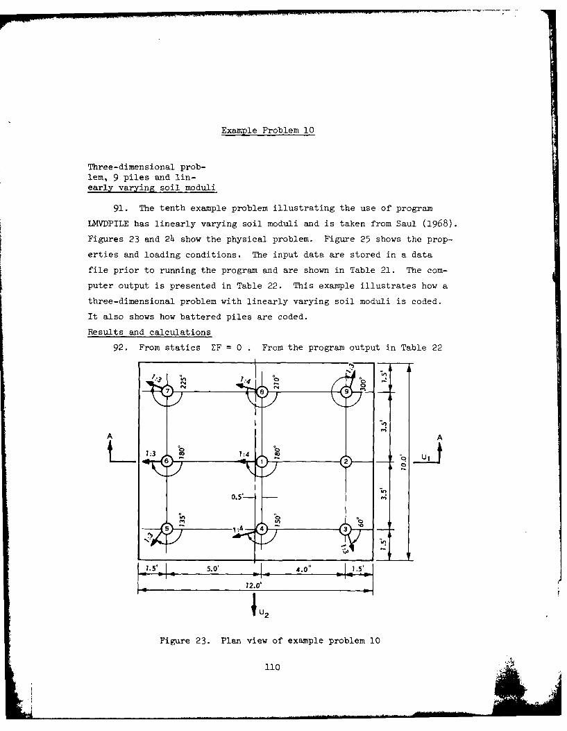
Example Problem 10

Three-dimensional prob-lem, 9 piles and lin-early varying soil moduli

91. The tenth example problem illustrating the use of program

LMVDPILE has linearly varying soil moduli and is taken from Saul (1968).

Figures 23 and 2h show the physical problem. Figure 25 shows the prop-

erties and loading conditions. The input data are stored in a data

file prior to running the program and are shown in Table 21. The com-

puter output is presented in Table 22. This example illustrates how a

three-dimensional problem with linearly varying soil moduli is coded.

It also shows how battered piles are coded.


92. From statics EF = 0 . From the program output in Table 22

In 1:4

7'

A A

II

I i.5~ ~4.0"

14 72.0'

Figure 23. Plan view of examrple problem 10

110

15'5.0' 4.0' .

.

/ 1 U1

Figure ~ ~ 24 eto - o eapepolm1

1,= 211.9 in. K =l.0h31 3

1 2 211.9 in. 4K 4 7063.3

Area = 16.1 in. K = 0.5445

Length = 120.0 ft K 6=0.5*44

Loading Q 3Q 5QCase -(kips) (kips) (kips) (kip-ft) (kip-ft) (kip-ft)

1 200.0 100.0 1500.0 1000.0 1*000.0 416.667

Figure 25. Properties and loading conditionsfor example problem 10

111

Table 21


GroupIA 1MOO6 EXAMPLE PROBLFM NO. 1IB 10010 SLD CPVCK PR03LEM NO. 2 -SX'L2A 10020 32B 19030 9 1 1A 10040 2 100-.e0A 10050 1 9 12e.ee0 2

4c 16060 211.900 211.90e 16.1z0 1.202 1.005A 1007 45C 10080 3060060.0006A 1T096 16B 1010 1.000 1.567 2.600 1.043 7063.306 0.544 0.544

10110 560.00 333.33 333.33 500.Vg 363.33 333.33 C.Zo lee.[VSA 101260

10 10130 4.0eee lFe.k o0 e. 1.10140 0. 0. 4.5 0 0. e.10150 3.-0e e.e00 4.500 3.5 e e.10160 4.e00 156.z66 0.5 0 3.560 0.10176 3.200 135.M, -4.513 3.tee 0.10180 3.60 1;0.20e -4.5ee 0. ?.1190 3.00e 225.000 -4.5/0 -3.500 0.1?266 4.V0 210.V0 e.576 -3.500 0.10210 3.600 302.00 4.51e -3.2 0.

1i 1022e 20Z.0 6 100.00 1500.006 1060.066 4006.C0 41Z.67

112

Table 22


EXAMPLI PAOUtTM NO. 19SL? C?.C! PROBLEM1 NO. 3 - SAUL

NO. O PILES - 0 MATRIX IS CALCULATID FOR ZACP PILE

1. TABLE OF PILT AND IOIL DATA

PILE NUMVPOS

1 9 1 - 3.30' 3 PSI IX - 211.90 IN**4 IT - 211.90 IN**4AREA - 15.1 IN*? I - 1.00 IN T - 1.0e INL-NGT? - 120.0 ?TT ES - 100.003T.1 - 0.567 1' X? 2.0000 W3 - 1.043014 -7063.3008 [5 - 0.5440 76 - 0.544@

ALLOVAPLT': COMBINED 3)NDING FOR TENSION - 500.000 ZIPSMOMENT ABOUT MINO AXIS ?OR TENSION - 333.330 ZIP-FTMOMENT ABOUT MAJOR AXIS P0! TENSION - 333.330 ZIP-PTCOMBINED l'E4DING FOR CO'PRESSION - 500.000 ZIPSMOMENT ABOUT MINOR AIlS ?O COMPRZSSIO4 - 333.330 ZIP-VTMOMENT ABOUT MAJOR AXIS ?OR COMPRESSION - 333.330 ZIP-FTCOMPRTSIV? LOAD - COO.300 KIPSTYNSILE LOAD - 100.000 KIPS

T? I MATRIX 1O1 PILES 1 TFROUGR 9 IS

0.750% 97 0. 0. 0. 0.267. 07 0.S. 0.7!PT 35 0. -0.282t 07 0. 0.S. 3. 0.0711 06 0. 0. 0.P. -0.?t0" Py 9. 0.1P2T 39 0. 0,0.262E 07 S. 0. a. 0.1021 09 0.0. 0. 0. 0. 0. 9.701E @7

2. TAPL' OP PILE COORDI4AT'S AND BATTER

PILT NO. HATTER ANGLP Ut(PT1 02() U3(?T1 4.30 10. 0.500 0. 0.

S 'qTICL 0. 4.500 0. 0.3 5.qs F . 4.530 3s.50 0.4 4.00 150. V.509 3.500 0.

1 .00 135. -4.!430 3.500 0.0 3.P3 190. -4."0 0. 0.

7 3.0 225. -4.5 0 -3.500 0.a 4.0 210. 0.5@0 -3.508 S.9 3.P0 300. 4.500 -3.500 0.

3. STIt PSM MATRIX S V'OR TY 9TRUCTUR

F.9112 06 0.732--03 -0.6162 0,1 0.3131 90 -0.8031 07 0.6251-410.977T-83 O.A41! 06 0.195w-02 0.6961 V? 0.250E Of 0.1771 07-6.630' 0' 0.3911-02 0.3 87 0.568r 0 -0.11!T 00 -0.3751 Of9.25"?O 0.048! 07 O."01T O0 0.R401 10 0. 0.057! 09-0.P03! 07 9.01 00 -0.11t 8 O.e0' 02 0.12S! 11 0.201 020.156 00 9.1'?' 07 -0.5931 O0 0.857E 09 0.320? 02 0.3057 10

IA 7t1l1ILITT MATWI1 P FOR TW STRCTURE

0.120145 -P.1441-14 0.13'7-96 -0.53 4-1 0.70.7 9 0.5131-19-0.15 0-14 9.1201-05 -0.604E-15 -8.9M09-9 -0.2309-16 -0.4321-090.1371-46 -0.9?5-15 3.14T-0 0 . @.1M6-160 .'C4!-09 0.2441-16

-0.3921-10 -0.93t'"-09 -'.198P-16 0.1231-00 0.6221-19 -0.3410-109.878t-09 -0.1721-18 0.164T-99 -0.I67-IA 0.7800-10 -0.06 7-14

-0.3351-10 -0.4321-09 0.3140-16 -0.341R-19 -8.8281-18 0.1381-09

(Continued)

113


~*e**** LOADING CONDITION 1 000*00"

4. MATRIX O APPLIE! LOADS Q (MIPS r. FV)

Q1 0' 91 Q4 Q5 Q6200.000 100.009 1500.000 1000.000 40e0.60 416.667

5. STRUCTUIE DEFLECT10NS (INCHES)

DI D2 D- D4 D5 DSF.48 00 3.106E '0 0.332! 00 0.1221-02 0.4361-62 0.1242-02

6. PILE DZPLOITIONS 4LO11 PILE AXIS (INC9ZS)

PILE X1 z' IS 14 X8 361 -0.!4Q' 00 -2.114? 00 9.1771 00 -0.148t-02 -0.4-361-02 0.90!-032 1.490 00 0.173E 14 0.952E-01 0.132M-02 0.436Z-02 0.124F-023 e.333E 00 -e.iOlP 00 0.255E 00 0.3761-02 0.1150-02 0.256E-024 -0,89 ,' 70 -0.317E -0 @.267E 00 0.793V-03 -0.4381-02 0.147F-02

-0.4 1 02 -0.37 - O 0.49-r 00 0.172-02 -0.394-02 0.188F-02a -0.542! 00 [email protected] 0.382t 00 -0.154t-02 -0.4367-02 0.789F-037 -0.55" 00 0.354E0 20 0.358? 30 -0.413V-02 -0.222E-02 -0.7220-048 -3.5717 J0 0.1?2r 10 0.11? 00 -0.3430-02 -0.316E-02 0.4175-0390.1007 091 0.554S '0 0.799E-6l -0.'3P02,? 0.323F-02 0.1?71-03

7. PiI! POlCES kLONG PILE AXIS (LIPS I F!T)

PIL P1 72 P3 P4 r, P6 CV7TR FAILUREC1 00 CO ?I

1 -52.443 -4.660 118.!-77 2.319-185.527 0.533 0.802 48.003 Q.8211 63.A88 -19.266 172.e20 0.728 0.701 25.657 -31.606 171.1*1 120.606 83.134 1.506 0.954 -41.1'- -25.81! 1'9.317 81.059-153.219 0.867 1.06 F5 -44.8q3 -29.717 332.913 99.416-160.382 1.104 1.45 T-59.533 1.074 256.359 -14.844-206.142 0.4C4 1.18 F

7 -47.167 '7.34' 240.492-139.9e'3-153.992 -0.043 1.3f TA -51.049 21.R48 79.427 -89.585-172.434 9.245 0.949 15.951 5.443 5.626-172.40A 70.896 0.102 0.84

TOTAL NO. rAILUR'S - 4 LOAD CASE I

B. PILE rO4CES ALO4r, STRUCTURE AIlS (KIPS , FZOT)

PIL '1 F' P3 V4 7! M61 22.118 4.'eP 127.7-6 -2.379 185.5'7 -0.0462 4.031 0.091I 63.88 -:9.66 172.620 a.72q3 6.6f1 52.11- 154.202 -14."? 141.141 -36.739

4 9.977 24.04o

183.681 8.324 172.116 -19.819. -23.322 65.140 330.021 4e.470 180.344 -30.3916 -'4.,9 -1.074 262.279 13.36 [email protected] 5.13!9 4."'1 -48.54P 2&3.066 -15.023 202.741 44.2018 37.131 -7.91 q9.437 -11.002 102.758 21.9659 59.731 -2.57? 45.830 -20.3A7 177.06A 54.617

SUM 268.#0@ 213.000 1500.e@9 1000.0020 4000.000 416.667

. . . . .. . . .. .. .. .. . . . . . .. . . . . .. . . .. .. . . . . .

this can be shown. For example, for a 200-kip applied horizontal load

in the U1 direction

I = Q1

where

F1 = horizontal pile force along the structure axis

= applied horizontal load in the U1 direction

EF1 = 22.12 + 48.00 + 66.7 + 9.98 - 23.32 - 24.59 + 4.27 + 37.13+59173

EF1 = 200.0 kips

Similarly

EF 2 -= Q2

where

Q2 = applied horizontal load in the U2 direction

EF2 = 100.0 kips

EF3 = Q3

where

F3 = vertical pile force along the structure axis

Q3 = applied vertical load in the U3 direction

EF3 = 1500.0 kips

These results agree with the computer program results.

93. Manual calculations for this example are presented in Saul's

(1968) paper. The computer results presented in Table 22 agree closely

with the classical method results. For example, a comparison of the

moments about the U -axis (F4's) is shown below:1

F4 fromPile Computer Saul'sNo. Output (kip-ft) Example (kip-ft)

1 2.319 2.312 -19.266 -19.253 120.696 120.68

(Continued)

115

A1 from]Pile Computer Saul'sNo. Output (kip-ft) Example (kip-ft)

4 81.059 81.03L5 99.1416 99.386 -14.844 -14.857 -139.903 -139.888 -89.585 -89.589 -172.4o8 -172.36

116

Example Problem 11

Three-dimensional problem, 60 pileswith linearly varying soil moduli

94. This example prob)lem is a three-dimensional system with 60

piles. The physical problem for this example is shown in Figure 26.

The properties and loading conditions are shown in Figure 27. Table 23

shows the data file saved prior to the run. The computer output is

presented in Table 24.

95. This example was run to verify that the computer results agree

with the St. Louis District's program.


96. The computer results shown in Table 24 agree closely with

those from the St. Louis program output. For example, for pile 1 for

load case 1, the pile forces along the structure axis from Table 2~4 are

F1 = 42.305 kips

F 2=0.0 Rips

F 3= 120.806 kips

F= 0 Rip-ft

F 5= 0 Rip-ft

F 6= 0 kip-ft

The St. Louis program produced

F 1= 42.3 Rips

F 2= 0.0 Rips

117

1 3 1 1 3 :3

1:31:3 r.

ORIGIN

1:3 3 1 31:3 ,:

1-1133- 1:3 t,

U 2 8

Fiur 26 Phsia prole 1or exml rolm1

7-3 73 1-31:318

Properties

E = 0.3 x 107 psi K1 = 0.411

KS = 2.000 pci K2 = 0.542I, = 5461.333 in. K3-K6 = 0.0

12 = 5461.333 in.

Area = 256.000 in.

Length = 60.0 ft

Loading l Q4 Q5 Q6

Case (kips) (kips) (kips) (kip-ft) (kip-ft) (kip-ft)

1 1207.5 0.0 3113.25 0.0 4825.5875 0.0

2 1454.25 0.0 1683.15 0.0 -2743.5342 0.0

3 1825.95 0.0 875.5 0.0 -5779.62 0.0

Figure 27. Properties and loading conditions for example problem 11

F3 = 120.8 kips

F4 = 0.0 kip-ft

F5 = 0.0 kip-ft

F6 = 0.0 kip-ft

These results agree very closely.

119

Table 23


Groupi IM: EXAMPLF PROBLEM NO. 11

1B 10010 TECH?-VFR4ILION OUTiLFT srRUTUq= 7.17 ri SPACI',2A 10020 32B 10030 60 1 3

10040 2 2.0A 10050 1 00 i 24C 10060 5401.333 5'.E1.333 256.00; 11.700 1.025A 1007e 45C 10080 00000.200 ___________

6A 10092 1

6B 10100 0. L.411 0.5,0 0. . 2.7 10110 268.9k 59.7Z 59.7e 2E-.E t9.7; 59.7' I5. 0. 29A 10120 010 10130 3.MoO e. -1i.25L, 50.17 e-

10140 3.M00 b. -3.75e 50.17, Z.10150 3.000 0. 3.752 E0.170 e.10160 3.207 0. 11.250 50.170 0.10170 3.00e 160.000 -11.25Z 43.20e 0.10180 3.000 180.000 -3.750 43.-00 0.10190 3.00e 180.000 3.7?2 43.200 0.10200 3.000 0. 11.250 43.Z00 0.10210 3.000 P. -11.250 3 .832 2.10222 3.220 0. -3.751 .5.&33 e.10230 3.020 e. 3.75e 35.'33 0.10240 3.200 0. 11.25, 35.833 0.1025, 3.000 180.000 -11.250 28.F67 0.1026y 3.0 180.000 -3.751 29.867 4.10270 3.000 180.000 3.75V 28.367 e.10280 3. oO 0. 11.250 28.-67 2.10290 3.000 2. -11.25 21.50 0.1030.0 3.000 2. -3.751 21.t00 0.10311 3.000 Z. 3.75W 21.!10 e.1032e 3.000 e. 11.75P 21.520 2.10330 3.ZO0 180.000 -11.2t? 14.333 0.10340 3.000 181.000 -3.752 14.333 2.1035o 3.000 130.000 3.75o 14.333 0.10360 3.000 0. 11.25Z 14.333 0.10370 3.000 e. -11.250 7.171 A.10380 3.200 (. -3.750 7.170 0.10390 3.ze0 0. 3.7E0 7.170 0.10400 3.000 e. 11.25e 7.17Z 0.10410 3.h00 180.000 -11.252 0. e.10420 3.200 1E0.000 -3.752 0. 2.10436 3.00 180.100 3.75 0. e.10440 3.000 0. 11.252 e. e.1e45Z 3.e,0 e. -11.2t- -7.17 1.10400 3.t00 0. -3.752 -7.170 e.10470 3.200 0. 3.75e -7.17e 0.10480 3.022 2. 11.25 -7.17C P.10490 3.200 10.o00 -11.250 -14.333 e.10500 3.900 180.e00 -3.751 -14.333 0.10510 3.000 1-I.e00 3.752 -14.337 e.

10520 3.100 P. 11.25? -14.332 0.10530 3.oo 2. -11.250 -21.t20 0.10540 3.000 Z. -3.750 -21.500 0.10550 3.000 0. 3.750 -21.530 Q.1050 3.000 0. 11.252 -21.5200 2.10570 3.000 180.000 -11.252 -28.6C7 e.10580 3.00 180.000 -3.750 -28.E67 0.10590 Moo0 160.00e 3.7fe -718.CC7 e.10690 3.00 0. 11.25 -28.667 2.10010 3.000 0. -11.250 -35.333 0.10020 3.2a0 e. -3.750 -35.:37 .10630 3.O0 0. 3.750 -3-.EZ3 0.1064 3.00e 0. 11.2!2 -35.E33 0.10650 3..00 130.000 -11.e.0 -43.. 0 2.Ml066 3.200 180.00 -3.750 -43..00 0.10070 3.O00 180.0e0 3.7t0 -43..20 e.10680 3.e0 e. 11.210 -43.-00 ?.106906 3.e00 2. -11.2s: -152.17 0.10700 3.000 0. -3.75' -50.17 9 0.

10710 3.200 e. '.7t0 -50.172 e.10720 3.e0 e. 11.2!V -50.17, V.10730 1207.!0e 0. 3113.25L C. 482t-M7 .

11 10740 1454.250 0. 1683.150 0. -2743.5Z42 2.1075 182t.-,5o e. 875.500 8. -5779.622 1.

120

Table 24


EXAMPLE PROBLEM NO. 11TECHE-VERMILION OUTLT SU1WTUxi. 7.17 ,T SP,.CIN6,

NO. 0' PILES = 6v MATRII IS CALCUL,.TRD FOR EACh PIL.

1. TABLE Of PILE AND SOIL DATA

PILI NUMBERS

1 60 - .0.30 (7 1PSI 11 - 5.61.33 IN* IY - 5461.33 IN*04ARZA - 256.0 IN**2 I . 16.00 IN 7 : 16.00 INLENGTH - a .0 FZIT ki z 2.006K1 = 0.4110 £K=0. 3 = 0

ALLONARLES: CCMhINEb ziNDIN- :OR TENSION 268.800 KIPS

MOMENT ABOUT MINOR AXIS iCR TANSION - 59.700 LIP-FTM.ViXNT *BUT MAJOR AXIS f0k TENSION = 59.700 lIP-FTCOMBINED SENDING FOR COMPR.:SSION = 268.860 KIPSMOM NT ABOUT MINO AXI-S FOR COMPR.ASSION : 59.700 vIP-PTMCMNT BOUT MAJOR AIS Uk COMV.PRESSION 59.710 lIP-F?COMPRBESIVI LOAD

= 15806 KIPS

T.NSILR LOAL - 148.880 KIPS

THE B MATRIX JCR PILES 1 TAROUGA 6, IS

0.7591 04 0. 0. 0. 0. a.0. 6.75ioi 04 0. J. 0. 0.0. 0. 9.533y .6 0. 0. 0.0. 0. 0. 0. 0. 0.

0. .. 0. 0. 0. 0.0. 0. 0. 0. ,0. 0.


121



PILL NO. BAffLE ANGL. U1 (1) UctkT) U3 (J?)

1 3.00 0 -11 .250 50.170 0.2 3.00 0. -3.75" 50.170 0.3 3.0 0. 1.?O0 50.170 0.

3 -300 0. .20 50.174 0.3.00 10. -11.Zb, 43.006 0.

6 3.00 160. -3.750 43.00 0.7 3.00 180. 3.?7D 43.006 0.8 2.00 0. 11.23 43.000 0.S 3.00 0. 211.2 3b.d3

3 0.

10 3.00 0. -1.250 35.cs33 0.10 3 .O 0.W. -3 .75.4 0. d33 0.11 3.00 0. 3.750 45.d33 0.12 3.00 0. 1 .25 55.d33 0.

13 3.00 Ida. -11.250 28.o67

0.14 3.00 180. -3.756 ;c .7 0.15 o.00 190. .5.75o c-.607 c16 3.00 0. 11.:30 a.oo? 0.17 3:.! 0. :-11.20 2.-,

0 0

18 3.0. 0. -3.75. 21.-4v 0.15. 3.00 0. 3.750 .1.500 0.20 3.00 0. 11.250 21.00 0.21 o.00 180. -11.-50 14...33 0.22 3.40 180. -. 75o 14.333 0.23 3.00 180. 3.70 1I .333 0.

24 3.00 0. 11.2b 14.333 0.

25 3.00 0. -11 .t0 ?.178 0.26 3.00 0. -3.?DO 1.170 0.27 .oo 0. 3.7to 7.170 0.28 3.d 0 0. 11.2tO 7.170 0.

29 3.0 180. -11.2o, 0 . 0.3V 3.00 180. -3. 75o 0. 0.31 2.00 180. 3.750 0.32 3.oO, 0 1'12.. 0. 033 3.00 0. -11.250 -?.174 0.

34 3.00 0. -3.750 -1.170 0.35 3. t 0. 3.750 -1.170 0.36 3.00 0. 11.250 -7.170 0.37 o.0 180. -11.2:0 -14.333 0

3C 2.00 180. -3.750 -14. 33 0.39 .5.00 150. ..750 -1t.333 0.40 3.04 0. 11.2b0 -1.333 0.41 3.00 0. -11.250 -21.50 0.42 3.Oo 0. -3.7b50 -21.00 0.43 a.0 0 3.750 -i1.500 0.44 3I.0 0. 11.250 -21.500 0.45 3.0 1o0. -11 .250 -zB.867 0.46 3.0 lo0. -3.750 -Z8.o67 0.4? 3.00 lo. 3 .75 -28.o67 0.48 3.00 0. 11.2.4 -20.u0

7 0.

49 3 .60 0. -11 .2:0 -35.ao3 050 3.00 0. -).7:,o -35.do3 0.51 .00 0. .-.?50 -35.133 0.52 3.o. 0. 11.±0 -35.833 0.53 2.0 loU. -11 .2, -43.000 0.54 3.h0 180. -3.75o -43.000 0.t5 3.W.0 180. 3.70- -43.400 0.56 3.00 0. 11.2± -43.000 0.57 3.00 0. -11 .250 -50.170 0.58 3.60 0. -3.750 -e.11i 0.

59 3.00 0. 3.750 -50.170 0.60 3.w@ 0. 11.25.0 -50.110 0.

•**.**.*.******************s***fln*af~.fel~nl.********.lf* .sm.sne.

3. STI INlSS M.TaII 5 125 TH.; STU.4TUh-

0.361i 07 -0.21o,-62 0.Zo4 07 0.1±0- 02 -0.29 8 , 0.7001 01

.:211#E-02 0.455. . a 0.O,7ro2 0.8±-.? aol, e40 0547i-010.2841 07 0.6b7 .02 o:,os0± Bo0320 .2 0.501L,0 0.±000 010.1608 02 0.18,8-.7 0.3:,. 02 0..9±, 13 0.5120 03 -0.5231 12-0.20n1 9 0.loo0 40 0. 0.42. If ,0.:±,2, 12 0.126L .40. 0.oz0 , -01 Oo.Oz. 01 -0.523, .2 O.o441 03 0.5038 12

3A JLUIMILIT2 1.1,IT 1 1O TH. STmJCTUE.

0.k30-06 -. Ibti.-14 0.32±-47 0.401.-1 0.o32,-0. -0.7110-1?0.1841-1 4 0.220±-o -0.6,,1.-15 -0.6±3.-I.l .. 401 -0-.7o-1.

-0.311-7 -.1518-5 0.l~±07 0.21..1- .332L-10 -0-c74i-18-0.127j-17 -0.llcr-s -0.±ole-ld 0.sl.-12 -0.27.-20 0.302E-120.3371-08 -0.-46±-lB -0..53-10 -0.-47-2.0 4.-77-11 -O.184t-fl-0.1231-17 -0.4340-1± -o.d.-1u *.302.-1,d -. 6d-20 0.2301-11


122


*S****** LO&DING CONDITION 1 ,,0"000

4. M&.T81X S APPLIZI. LOADS (OIP5 . P. ,TI

Q1 W4 ,,- 9, 61207.500 0. 3113.2W0 0. 4825.588 0.

5. STRUCTU6. nIFLECTION % INH-&S

D1 15 1. L. D0.3171 (00 0.02-. .7u.?0-01 -0.340.-11 0.522L-03 -4.105Z-10

6. PILE DELOTIONS ALONL PILS AX1b (INhCHS)

PILL 21 2.. .. 0a I. X61 0.2541 00 0 .150f0-WC 0.24o. 00 0. o182;-13 0 .5226-"3 -. 1100-102 0.2691 00 0.55.6..-08 0.1951 .0 0.o8Ii,-13 0.522,-03 -0.1OE-103 0.284E 00 -0.3921-08 e. 11 bIA 0 0. .10.-2 .5;e2x-03 -0.1100-104 0.299 00 -0.134.-08 0.146-' .06 O.V19,-13 0.5022--03 -0.1102-105 -0.3481 00 -0.213_.-08 0. o 3E-Z1 0.753.-11 -0.522i-03 -0.o560-116 -0.3331 00 -. 118 . -0.528.-O0. 0.753--11 -0.522.-03 -0.8560-117 -0.31d4 00 -0.23'-0 -. 6-01 0.75-;-22 -0.522,x-0O -0.856Z-118 0.2991 00 -0.134;-8 0.10o0 00 0.919L-13 0.5e2i-03 -0.1100-109 0.2541 .0 0.1500-08 0.?40Z 00 0. 19-6-13 0.5221-03 -0.1101-1010 0.2690 00 0.55.2£-08 0.19b. 00 0.1199-13 0.522F-03 -0.1102-1011 0.264Z 00 -0.392L-09 0.1510 00 0. 19;- 13 0.522 -3 -0.1100-1012 0.2991 00 -. 134-00 0.10o -00 0.to10-13 0.522.-03 -0.1100-1013 -0.3481 00 -0.213E-0t 0.33.;-01 0.753,'-Il -0.522E-03 -0.8560-1114 -0.3331 .0 -0.110.-G8 -0.5;:, -02 0.753F2-11 -0.5Z22-03 -0.8560-1115 -0.318t 00 -0.230-0 -04890-81 0.731,-I 0 -. 502-03 -0.856Z-1116 0.2990 00 -0.134E-0 0.10o- 60 0.V19L-13 0.522E-03 -0.110E-1017 0.254Z 00 0.1502-0d 0... 00 0.9194-13 0.522,-03 -0.1100-1018 0.269E 00 0.553Z-9S 0.1. 00 0.61,-13 0.522i-03 -0.1100-1019 0.284i 00 -0.392Z-09 0.151& 0 0.919.-13 0.522.-03 -0.1100-1020 0.291 00 -0.1349-0d 0.1060E 0 0.194-13 0.522.-03 -0.1100-1021 -0.348F 00 -0.213.-0e 0.3w3t-d1 4.753z-11 -0.5220-03 -0.8560-1122 -0.333L w0 -0.1180-0d -0.520d-02 0.75.3-11 -0.522i-03 -0.8560-1123 -0.3181 00 -0.23o.-01 -0.4.09-41 0.753i-11 -0.522Z-03 -0.8560-1124 0.2994 00 -0.13,.-. 0.10.1 0 0. 1.9-13 0.522"-0 -0.1100-1025 0.25E 00 0.1500-08 0.2406 J0 0.819-1.5 0.5222-03 -0.1100-1026 0.26982 00 0.5530-19. 0.150 ,00 W.9192-13 0 .522,-03 -0.1100-1027 0.2840 00 -0.3920-.9 0.151. 00 0.V19.-13 4 "-'2,-03 -0.1100-1028 0.2992 00 -0.1340-0d 0.10o 0.. 0.019-13 0.!m2.-06 -0.1100-1029 -0.3461 00 -0.2130-08 0.00-81 0.7W42-11 -0.522,-03 -4.856f-1130 -0.333i 00 -0.1162-08 -0.5280"-V 0.7531-11 -0.5i"2.-03 -0.6560-1131 -0.3190 00 -0.238-"6 -0.4990101 0.531-11 -0.522-03 -0.6560-1132 0.2990 00 -0.1340-08 0.1062 00 0.ol92-13 0.522t-03 -0.1100-1033 0.2540 00 0.15O.-08 0.24. 0 0.192-13 0.b22-03 -0.1100-1034 0.2690 00 0.55.2-O 0.15b .0 0.180-13 0.522,-03 -0.1100-1035 0.2984 00 -0.392Z-08 0.151i 00 0.19. -13 0.522 -03 -0.110E-1036 0.2990 00 -0.213,:-08 0.10o- , 0.910.9-13 0.522b-03 -0.110-1037 -0.3400 00 -0.21d&-08 0.393U-01 0.7530-11 -0.522,-03 -0.856E-1138 -0.333t 00 -0.110--08 -0.5Z66-02 0.753-1l -0.522,-03 -0.862-1139 -0.319 00 -0.1382-08 -0.462-01 0.71 3-11 -0.522.-03 -0.8560-1140 0.2S99 00 -0.1340-08 0.106 . 00 0.119-13 0.5221-03 -0.1100-1041 0.2540 00 0.1b0-08 0.240L 00 0.919i-13 0.522--03 -0.1101-1042 0.268 00 0.5530-06 0.165 .0 0.J1-13 0.522-93 -0.1100-1043 0.284 00 -0.1v2,-02 O.15kL 00 0.6190-13 0.5221-03 -0.1100-1044 0.26460 00 -0.134-2 0.106 ; .0 0.7o81-13 0.522.-03 -0.1100-1045 -0.340 00 -0.2130,-08 -0.5.0-01 0.753A-11 -0.5Z2&-03 -. 8560-1146 -0.333 00 -0.1132-0 -0...dxl0 0.7532-11 -0.522.-03 -0.8560-1147 0.3190 00 -0.380-06 -0.494-01 0.753-11 0.521-03 -0.8560-1148 0.254E 00 -0.1540-0e 0.120 00 0.619-13 0.52-03 -0.1100-1049 0.254t 00 0.150 0- 0.24.6 O 0.d19,-13 0.522.-03 -0.1101-1050 0.2680 00 0.32-06 0.1652 00 0.9191-13 0.5220-03 -0.1100-1052 0.284t 00 -0.692i-09 0.13A1 .0 0.t196-13 0.5Z2-03 -0.110E-1052 0.289 00 -0.134L-0e 0.100. .0 0.8.-16 1. "0.5;22-03 -0.1100-1053 -0.3489 00 -0.213.-08 -0.35 -,2 0.753.-11 -0.522.-03 -0.8561-1154 -0.331i. 00 -d. 116-08 -0.5486-42 0.73 .- 11 -0.5.2i2-03 -0.856E-1155 -0.3182 00 -0.238006 -0.09£ 2-01 0.75.5-11 -0.5i22-03 -0.560-1156 0.26v8 00 0.1340-40 0.1.2 00 0.919-13 0.5Z2.-03 -0.1100-1057 O.2560 0 0.2509-08 0.40., 00 0.618.-13 0.5,2-03 -0.1100-1058 0.2660 00 0.553Z-06 0.1,1 00 0.18-13 0.5228-03 -0.1100-1059 0.2b40 00 -0.3$02t-0. 0.1b11 ;0 0.626,-13 0.be2203 -0.11009-1060 0.289t 00 -0.134i-08 0.100 00 0.419-13 0.52.-03 -0.1100-10

(Continued) (Sheet 3 of ]1)

123

Table 2h (Continued)

7. PILE FORCES ALON PILL AXIS ,J12, . filJ| )

PILL 11 22 f, .F C.FTR FLILURLCA BU CO TZ

1 1.931 0.00 I'1.d85 .A. 0. 0.4b

2 2.044 0.00 104.24d 0. 0. 0. 1 .313 2.157 -0.000 d0.463 0. 0. 0. 0.304 2.270 -0.000 56.6b' 0. 0. a. 0.21

5 -2.638 -0.00 20.957 0. 0. 0. 0.066 -2.525 -0.000 -2.019 0. A. 0. J.01

7 -2.412 -0.000 -26.5"1 0. 0. 0. 0.108 2.270 -0.0,60 56.6b7 0. A. 0. 0.219 1.931 0.00 127.9o5 0. 0. 0. 0.48

10 2.044 0.000 104.2we 0. 0. 0. 0..,A11 2.157 -0.-00 o..4 3 0. 0. 0. 0.30

12 2.270 -0.000 56.657 0. 0. 0. 0.21

13 -2.636 -0.000 Z0.957 0. 0. 0. 0.0b14 -2.525 -0.000 -2.dib 0. A. 0. 0.01

15 -2.412 -0.000 -20.594 0. 0. 0. 0.1016 2.270 -0.000 56.65? . 0. 0. 0.2117 1.931 0.000 127.985 0. 0. 0. 0.49

18 2.044 0.00. 104.e A. 0. 0. 0. 0.69 L

19 2.157 -(6.000 60.433 0. 0. 0. 0.30

20 2.270 -0.060 36.657 0. 0. A. 0.21

21 -2.6, --. 000 20.87 0. 0. 0. 0.0

22 -2.525 -0.000 --.818 0. 0. 0. 0.0123 -2.412 -0.000 -2.5a,4 0. 0. 0. 0.1024 2.270 --. 000 56.6b7 0. 0. 0. 0.21

25 1.931 0.000 127.965 0. 0. 0. 0.4826 2.044 0.00 104.20V 0. 0. 0. 0..27 2.157 -0.000 *0.433 0. 0. 0. 0.3028 2.270 -0.0,0 26.657 0. 0. A. 0.21

29 -2.69 -e.000 20.9'7 0- 0. 0. 0.0o

3V -2.125 -0-M0 -k.61 d 0. 0. 0. 0.0131 -2.412 -0.000 -. 46.6"4 0. 0. 0. 0.1032 2.270 -0.004 t6.657 0. 0. 0. ..21

33 1.931 0.000 127.985 0. 0. 0. 0.4834 2.044 0.0.0 196.20W 0. 0. 0. 0.3935 2.15? -0.000 d0.463 0. 0. 0 . 0.30

36 2.270 -0.600 56.65'1 ,d. 1. a. 0.2137 -2.939 -0.000 20.95? 0. 0. 0. 0.09

38 -2.525 -0.00 -!.918 0. 0. 0. 0.0139 -2.412 -0.000 -,4o.5" 0. 0. 0. 0.10

40 2.270 -0.-00 56.o' - 0. 0. 0.2141 1.931 0.000 127.985 0. 0. 0. 0.48

42 2.044 0.000 104.20 o 0. 0. 0. 0.39

43 2.1b? -e.000 80.4-53 0. 0. 0. 0.30

44 2.2?0 -0.000 50.65? 0. 0. 0. 0.21

45 -2.638 -0.000 20.657 0. 0. 0. 0.0946 -2.525 -0.000 -2.618 0. 0. 0. 0.014? -2.412 -0.000 -2o.594 0. 0. 0. 0.1048 2.270 -0.000 56.657 0. 0. 0. 0.21

49 1.931 0.W00 127.865 0. 0. 0. 0.4950 2.044 0.000 104.20. 0. 0. 0. 0.39

51 2.157 -0.600 90.433 0. A. 0. 0.30b2 2.270 -0.000 56.657 0. 0. 0. 0.21

53 -2.638 -0.00 20.957 0. 0. 0. 0.0854 -2.525 -0.000 -2.918 0. 0. A. 0.01

55 -2.412 -0.000 -2o..54 0. 0. A. 0.1056 2.270 -0.000 56.657 0. 0. 0. 0.21

57 1.931 0.00 127.995 A. 0. 0. 0.4d

b8 2.044 0.000 104.20.. 0. 0. 0. 0.39

59 2.157 -0.000 J4.433 0. 0. 0. 0.30Of 2.270 -0.000 b6.657 0. 0. 0. 0.21

TOTAL NO. 1AILURiS 4 0 LOL CASE I

(Continued) (Sheet h of ii)

124

z I1


e. PILE FORCES ^LONG SKUCTURI AXIS 9lrSt F-PL,

PILE F1 F, i3 1 461 42.305 B.8Ja 120.-06 0. 0. B.2 3i.bb3 @.Joe 9t.210 a. B. W.

3 27.4b1 -0.-08 75.o3 8. 0. i.t 20.07 -0.099 b3.432 B. . .t -4.1zt 9.090 20.716 B. - B.6 ..287 0.-9 -1.87. B. a. B.7 10.6$08 -0.009 -24.4"? B. 4. B.a 20.0,c -B.BBB 53.032 B. J. B.9 42.3.5 8.0de 120.80o B. 0. B.

lB .4.k68.l B.0BB 98.21b B. 9, .11 27.481 -0.066 75."23 B. B. B.12 28.80 -0.dBB 53.432 B. B. B.13 -4.125 0.888 20.716 0. 0. 0.1t 3.28? B.009 -1.87 0. B. 0.15 10.698 -0.4B8 -24.%o7 6. B. B.18 2B.B7B -0.#BB 53.43- B. B. 0.17 42.3B5 @.'Jo 120.d46 B. B. B.18 34.893 8.88.) 9d.21b B. B. B.19 27.481 -6.8B.) 75.b.3 8. B. Z2B 2B.BB -. )ed 5,5..32 B. B. B.21 -4.125 B.0. 20.716 B. B. v. [22 3.287 8.080 -1.87 B. B.23 10.698 -0.66B -2A.4o7 B. B. 8.24 20.070 -B.BB b3..;3z B. . 1.25 42.385 J.81 128.80. B. . .28 34.b96 8.88 98.211 B. 8. a.27 27.481 -8.808 75.623 B. B. B.28 2B.B74 -0.989 53.j32 B. 8. a.29 -4.1U5 B.aBB 20.716 8. 8. B.38 3.287 B.0BB -1.87b a.31 1B.698 -0."@ -24.467 a. B. B.32 29.970 -8.-69 .3.332 8. B. B.33 42.385 ..goB 120.896 8. a. 8.34 34.,33 8.W88 98.215 0. 0. B.35 27.481 -0.BBB 75.623 0. 0. 0.36 20.07B -0..BB 53.832 0. B. 8.37 -4.125 8.888 Z41.71.6 a . a.38 3.287 0.08 -1.26% -. B. -.39 18.698 -9.099 -24..67 0. B. 8.48 a8.070 -9.08 53.032 0. 8. 141 42.385 @.@is 128.oa 2 0. 8. .42 34.893 8.888 ,8.21t2 0. 8. 8.43 27.481 -8.088 75.623 0. B. a.44 28.87) -8.188 5.3.832 8. 4. B.45 -4.125 8.888 20.710 0. J. 0.46 3.Z87 8.0 -1.87z1 8. 8. 8.47 18.698 -0.009 -24h.40? 8. 8. 8.48 20.097 -8.888 53.83, B. 8. 8.49 42.385 0.888 128.888 8. 46. a.58 34.893 0.08B 98.215 B. 80. 8.51 27.481 -8.888 75.523 @. 8. a.52 28.878 -8.888 53,032 8. a. B.53 -4.125 8.89 2h.71e . 0.o .54 3.27 8.888 -1.87Z B. . .55 18.698 -8.888 -24. 667 8. a. 8.58 28.878 -8.888 53.832 0. 8. a.57 42.385 8.888 128.886 B0. 8. 8.58 34.893 8.808 98.215 J. 8. 8.59 27.481 -8.888 75.6k3 8. 8. 8.68 29.870 -83.888 53.832 8. 9. .

SUM 1287.588 9.00B 3113.25o -86.881 482!5.587 -8.080


125


*S* LOADING COk.lTIOi 2 ine

4. MATRIX OF APPLIOD LOADS Q (LIPS 7 4c.]T)

Qi Q2 Q Q61454.250 0. 1683.150 0. -274 .54 0.

5. STRUCTUR' DUhLECTIONS (INCHLS)

It U. _,5 . 16 L 60.415E 00 0.154"-d 0.175E-01 -9.3,42:.-11 0.311.--.5 -0.1029-1ie

6. PILL DFLICIIONS *LONG PILl AXIS I1N ,;S)

1 0.395 00 O.,W2,-OL 0.1ksd 00 0.1644-12 0.311 Z-03 -0.1073-102 0 .3831 00 0.200f.-Jd W. 1 bt 00 0.164,;-12 0 .3114-0.5 -0.1071,-1o

4 0.401. 00 0.165.-0O, 0.10.E .0 0.164.-12 0.311,-03 -0.1071-105 -0.412L 00 -0.374.-0.G -0..7-41 0.687.-11 -0.311.-03 -0.8 5Z-116 -0.403i; 00 -0.82,;-08 -0.101. .0 0.687,"1-11 -0.311--03 -0.845L-117 -0.395t 00 -0.10£-00 -0.1281 00 0.687U-11 -0.311.-03 -0.8451-118 0.4011 00 0.165; -0 0. 106 00 0.164,;-12 0.6115-03 -0.1071-10f 0.375L 00 0.292,.-Jo 0.1088, 0- 0.164-12 0.311-03 -. 1071-10

10 0.3831 40 0.200i-0e 0.1.i 0o 0.164.-12 0.311i,-03 -0.107--1011 0.32& 00 0.10.o-08 0.135, 0 0.1642-12 0.311-03 -0.1070-1012 0.401i 00 0.165L -64 0.100L 00 0.164.-12 0.3111-03 -0.1071-1013 -0.412. 00 -0...74,-0' -4.747i-Il 0.6872-11 -0.3111-03 -0.845E-1114 -0.403L 00 -0.2824-00 -0.101 0. 0.687".-11 -0.311.-03 -0.8451-1115 -0.3(5Z 00 -0.1901-08 -0.12-1 0 0.687.-11 -0.311i-03 -0.845Z-1116 0.4011 00 0.16D,;-09 0.1o00 00 0.1641-12 0.311,-03 -0.107E-1017 0.3751 0 0.292E-00 0.1681 00 0.164,.-12 0.311.-03 -0.107E-1018 0.3831 00 0.2001-08 0.1o1' .0 0.164-12 3.311-03 -0.1072-1019 0.392i 00 0.100"-48 0.135L 00 0.164L-12 0.3111-03 -0.107;-1020 0.401L 00 0.1650-.w 0.1001 00 0.164.-12 0.311-03 -0.107E-1021 -0.412 00 -0.,7 .- 08 0.747-01 0.687U-11 -0.311E-03 -0.8'55-1122 -0.403i 00 -0.2d20-08t -4.101L 00 0.607.-li -4.311.-03 -0.8451-1123 -0.3%5Z 00 -0.1901-00 -0.1,oO 00 0.687-11 -0.311-03 -0.8451-1124 0.4011 00 0.16a,-06 0.10o, 00 0.164Y-12 3.3110-03 -0.107Z-1025 0.37 1 00 0.292i-0 0.108 10 0.164,;-12 0.3111-03 -0.107E-1026 0.3831 00 0.2909-06 0.161f 00 0.16,-12 0.311-0 -4.1071-1027 0.392N o 0.1081-0e 0.1,b .0 0.164j-12 0.3111-03 -0.10U.-1028 0.4011 00 0.165i-6 0.1000 )0 0.164.-12 0.311,-03 -0.1071-1029 -0.4121; 00 -0.5749-00 -0.747.-dl O.oO7-11 -4.311.,-03 -0.845E-1130 -0.403/ 00 -0.2d20-08 -0.1011 L0 0o0873-11 -0.311 -03 -0.845F-1131 -0.35b 00 -0.140i-08 -0.1;1. A0 0.687&-il -0.311,-03 -0.845E-1132 0.4011 00 O.195i-0. R.Lds 00 0.164&-12 0.31IL-03 -0.107E-1033 0.375i 00 0.2w2,-0O 0.108,. .0 0.164,.-12 3.311-03 -0.1071-1034 0.383f 0o0 0.2001-00 0.101, 00 0.164--12 0.311,-03 -0.1071-1035 0.3921 00 0.108,0-08 0.13Zi. 00 0.16".1-12 0.311.-03 -0.107Z-1036 0.4011, 00 0.165i:-d 0.1081 0,) 0.164-12 0.311--0. -0.1071-1037 -0.4121 00 -0.3749-48 -0.7t71-01 0.W8.-11 -0.3110-03 -0.8459-1138 -0.4031 00 -6.2 2-08 -. 101" 00 0.o870-11 -9.311,-03 -0.8451-1139 -0.395. 00 -0.1909-0d -0.IdO 00 0.687.-11 -0.3110-03 -0.8451-1140 0.4019 00 0.16t.,-06 0.1-.o 00 0.1644-12 0.311 E0' -0.107%-1041 0.3751 0o 0.Z12.-00 0.100, 00 0.164.-12 0.311-03 -0.107E-1042 0.38Z1 00 0.2000-0c 0.161- 0. 0.164i-12 0.311-03 -0.107Z-1043 0.,)24 00 0.O.0.;-Oo 0.145. j:0 0.164j;-12 0.311,-03 -0.1070-1044 6.4019 00 0.16b-OS 0.10, .0 0.164,-12 0.311t-03 -0.1071-1045 -0.4121 00 -0.474,-OU -0.147L-01 0.o87L-11 -0.311E-03 -0.8450-1146 -0.4030 00 -0.2o2g-08 -0.101k ,0 0.607"-11 -0.311,-03 -0.845E-1147 -0.395i 00 -o.1.03-00 -a.1001 00 0.687,-11 -. 3111-03 -4.6459-1148 0.4011 00 0.16is-ig 0.1.od. .0 0.164,-12 0.311.-03 -0.1071-1049 9.675N 00 0.2620-0, 0.168b . 0 0.164-12 0.311-0.5 -0.1071-1050 0.383i. Ow 0.200,-0e: 0.1.1. 00 0.1640-12 0.311,-43 -0.1071-1051 0.342. 10 0.10,0-0 0.135i 60 d.164,-12 0.311&-03 -0.1070-1052 0.401a 00 0.16.-.. 0.17,,. 00 0.164.4-12 0.311.-03 -0.1971-1053 -0.412. 00 -0.6 .7-02 -0.747- 1 0.oB7 -11 -0.311k-03 -0.8450-1154 -0.403i 00 -0.Z82i-0. -0.101,. 0. 10.08LW-. -11 1..0 -0.8451-1155 -0.305& 00 -0.190i-08 it.10 .e 0.oV-11 -0.311-03 -0.845i-1156 0.401i 00 0.16..-wo 0.10,0 10 0.1644-12 0.311-03 -0.1071-1057 0.315& 00 0.21o2g-od 0.1 E 00 0.164.-12 0.3110-03 -0.1071-105d 0.383& 00 d.200,.-dt! 0.1 t1t, Of 9.16-12 0.311i-03 -9.1079-10t9 0.%o2i Do 0.10.0-d 6.135. 0. 0.164-12 0.311.-03 -0.1071-106d 0.401i 00 0.165 - 1 0.10., . 0.1b4.-12 0.311-03 -0.107E-10

(Continued) (Sheet 6 of i])126


7. PILl 1CR,. "O FLL A,. kKP1. alP

PIL. 11 F, i3 1. k io CBFTR FAILUREC3 DU CO T

1 1..4 J. 100.,,/ 0. 0. 0. 0..72 2. 10 :.00 5.88o 0. 0. 0. 0.3..3 Z.977 7.100 h.744 0. 0. 0. 0.274 3.045 0.60 5.602 0. 0. 0. 0.2i5 -3.126 -0.000 -2.,.2, 0. 0. 0. 0.1b6 -3., 6 -0.,00 -54.0:1 0. 0. 0. 0.2,17 -4.i95 -0.000 -o8.140. 0. 0. 0.256 .045 0.00. .?.62 0. 0. 0. 6.216 .64, 0.000 100.0 0. 0. 0. 0..?

10 2.910 0.00 85.860 0. 0. 0. 0.3 -11 2.977 0.000 71.744 0. 0. 0. 0.712 3.0 45 0.,0 .,.6o2 0. 0. 0. /.2113 -3.12w -(.000 -39.059 0. 0. 0. 0.151 -3.062 -0.000 -5 .,O1 0. 0. 0. 0.2015 -2.95 -0.000 -0d.14.2 0. 0. 0. 0.2516 3.045 0.00. 57.602 0. 0. 0. 0.2117 2.843 W.00 100 027 0. 0. 0. 0.3710 2.610 0.0.e0 8.oSO . . 0. 0.32

19 2.977 100 71.7.4 0. 0 0. o.20 3.045 0..100 37.6, 0. ,. 0. 0.2'21 -. 129 -. 100 -36.859 0. 0. 0. 0.122 -3.052 -0.000 -54.001 0. 0. 0. 0.2023 -2.995 -0.00 -0_8.143 0. 0. 0. 0. '524 Z.045 0..00 ? .:6W2 0. 0. 0. 0.2125 2.64) 0.00.. 100.0? 0. 0. 0. 0.3726 2..10 0.040 c.88o 0. 0. 0. 0.3227 2.977 e.000 71.744 0. 0. 0. 0.2728 3.045 0.00 57.602 0. 0. . 0.2129 -3.129 -0.000 -31.854 0. 0. 0. 0.1530 -3.062 -0.000 -54.001 0. 0. 0. 0.2031 -2.95 -0.000 -. 1 2 0. 0. 0. 0.25

32 3.0*5 0.000 57.602 0. 0. 0. 0.2133 2.b43 6.000 100.027 0. 0. 0. 0.3734 2.610 0.0 5.o 0. 0. -. 0.3235 2.97? 0. 40 71.744 0. 0. 0. 0.2736 2.045 0.0.01 .1.6.2 0. . 0. J.2137 -3.1IZ9 -0.000 -39.8b 0. 0. 0. 0.1538 -Z.062 -0.000 -34.001 0. 0. 0. 0.2039 -2.995 -0.:00 -6.143 0. 0. 0. ..2540 3.045 0.000 a7.602 0. 0. 0. 0.2141 2.843 0.040 100.027 0. 0. 0. 0.3742 2.10 0.000 8:.886 0. 0. 0. 0.3243 2.077 0.090 71.744 a. 0. 0. 0.2744 3:.045 0.000 57.602 0. 0. 0. 0.2145 -3.12V -0.000 -3.856 0. 0. 0. 0.15

46 - .062 -0.000 -5 .001 0. 0. 0. 0.2047 -2.995 -0.000 -6o.143 0. 0. 0. 0.548 3.045 '.000 57.0 6 . 0. 0. 0.2249 2.843 0.000 100.027 0. 0. 0. 0.0?50 2.910 0.000 85.886 0. 0. 0. 0.3251 2.97? 0.000 71.744 0. 0. 0. 0.2752 3.045 0.000 57.602 0. 0. 0. 0.2153 -. 126 -0.000 -39.85w 0. 0. 0. 0.1554 -3.062 -0.000 -54.001 0. 0. 0. 0.2,55 -2.965 -0.000 -v).143 0. 0. 0. 0.2556 3.045 0.000 57.602 0. 0. 0. 0.41

57 2.843 0.o00 100..,27 0. 0. 0. 0.758 2.910 0.000 85.886 0. 0. 0. 0.3259 2.97? 0..00 71.744 0. 0. 0. 0.2760 3.05 0.000 5 .602 0. 0. 0. 0.21

TOTAL NO. 1AILUR.-S - , L,. CA.)

(Continued) (Sheet 7 of ii)

127

Table 2h (Continued)

e. PILl IOkCES ALONG STRUCTUI Allt ,KIx5 . PiT)

PILI F1 i4 J F 61 34. 0.000 93.9 0 0. 0.

2 2 .920 0.0 8 03.:5. 0. 0. 0.3 25.512 0.60 67.12i 0. 0. 0.4 21.10 0.0 5..6d. 0. 0. 0.5 1:.573 -0.000 -6..d44 0. 0. -.

6 19.981 -0.0 -D, .6o1 0. 0.7 24.3d9 -0.h0 : -63.699 0. . 08 21.104 0.00 53.683 0. Z. 0.

9 .3 0.00 9.3.vg 0. 0. 0.10 29.920 0.000 ao.56 0. 0. 0.11 25.512 0.J0, .7.121 0. 0. 0.12 21.104 0.00 5 .. 0. 0.13 11.573 -0.00 -36.14 0. 0. 0.14 19.901 -.. 00 -. 2o1 0. 0. 0.15 24.3o9 -0.oe0 -6..59 0. . 0.16 21.104 0.00 5...0

3 0. . 0.

17 34.320 0.000 9..99b 0. 0. 0.18 29.926 0.000 80.:u5 0. 0. 0.19 25.512 0.00 67.121 0. 0. 0.20 21.10. 0.000 5z.OOL 0. 0. 0.21 1b.573 -0.000 -56.d4 0. 0. 0.22 10.981 -0.000 -. 2o1 0. 0. .23 24.3.9 -0.0,0 -61.o99 0. 0.24 21.104 0.400 :3.6d3 0. 0. 0.25 34.329 0.000 93.99 -.. 0. 0.

26 29.920 0.60 019 0 . 027 25.512 0.00 67. 21 0. 0. 0.28 21.104 0.00. 53.6d. 0. 0. 0.29 1E.573 -0.000 -46.d24 0. 4. 0.30 159.961 -0.0,d0 -5 .261 0 . 0.31 e4.309 -0.0600 6.4.9 0.352 21.14 0.000 56 66 . .. 0..53 34.329 0.000 9.1. ,9: 0. 9. 0.34 29.920 0.000 80..56 0. 0. 0.35 25.512 0.000 67.121 0. 0. 0.37 215.57 -0.000 -36.624 0. 0. 0.36 21.104 000 53.b3 0 0. 0.37 15.573 -0.,690 -366b;4 0:0.

38 19.981 -0.000 -50.2,1 0. 0. 0.39 24.389 -0. 000 -63. 6 . 0. 0.

40 ;e1.104 0.00 53. bd 0. 0. 0.41 34.329 0.30k. .3. 9.. 0. 0. 0.42 29.920 0.00 a.35o 0. 0.43 25.512 0.040 67.121 0. 0. 0.44 21.104 0.040 53.683 0. 0.45 15.573 -0.000 -36.44 0. 0.46 19.981 -. 00 -50.2o1 0. 0. .47 24.389 -0.00 --63.: 9 0. 0.48 21.104 0.00 3.o3 0. 0. 0.49 34.329 ;.000 . ..69b 0. 0. 0.be 29.926 v4.000 od.15o W. -. 0.51 2t.512 0.000 67.121 0.. .52 21.10 1 0.00 5o.bo3 0. 0. 0.53 15.57 -0.000 -6..24 0. 0. 0.

54 19o.991 -0.000 -021 0. 0. 0.55 24.. o9 -0.000 -6 ..649 0. 0. 0.

56 21.10k 0.000 5 .ud 0. 0. 0.57 34.3o" 0.000 .*L.9o 0. 0. 0.

58 29.920 0.000 oj. 5 0. 0. -.

59 25.512 0.040 e7.121 0. 0.60 21.104 0...@a b3.6,3 0. 0. 0.

SUM 1454.250 -0.000 1663.1 6 -0.000 -0,4-1.534 -0.000

O*.....n.....s..,..........q~oe.e . .oSoo **U0oo **** *fl.p.oo*o******

(Continued) ( 8 of

128

r"Table 2~4 (Continued)

0*0000* LOADIN , ONLITION a ,

4. 647112 0F APPLIED 104 5 q 1KiS FLPIT,L

Qi Q 4, ' -- Q6162t.950 0. 875.5.50 0. -5779.626 0.

5. STRUCTUR DLIECTIONS k1h,;H8)

DI L2 -4 -40.5521 00 0.7E-08 0.23,j-01 -0.3u7s-il 0.325L-0o -0.11i-10

6. PILl LULECTION5 ,.LONG PILE .AIS 1N28,)

PILE 11 'c' A.. 14 L K61 0.5171, 00 0.4400--c 0.1.3E 0 0.2 0,-12 0.32, -03 -0.125E-102 0.1261 00 0.a32o-0e 0.xk 00 0.2,.-12 0.325.-03 -0.125b3 .b3b .0 0.225&;-0 0.156 0. 0. 2v6-12 0.325,-03 -0.125-14 .. 54.E 00 0.11ol-0A 0.110 00 0.290,-12 0.345--03 -0.125E-105 -0.5301 00 -0.549L-O -0.15 J0 0.787,-11 -0.3Z5.-03 -0.996L-116 -0.-120 00 0.M&ie -0.1n30 00 0.787f-11 -0.325-03 0.9966-117 -0.:1 , 00 -0.334.-Od -0.2I1k 0.. 0.787z-11 -0.35-03 -0.996E-118 0.545i 00 0.11o -0. 0.±l00 00 0.2'0,-12 0.325.-03 -0.12b-10

1 6 0.5170 0 0.03.-0o 0.1.3. . 0.4.0.6-12 0.325-03 -0.125E-10

11 0.5 5. .0 0.22 i-0o ,.133. 00 0.2J04-12 0.325i-03 -0.1254-1012 4.545. '0 0.1-*, 0.110i 0. 0.,0-12 0 .3d5-03 -0.125E-1013 -0.530. 00 -0.546,-to -0.1:52. 40 0.7 --Il -0 .32 D-"2 -0.9962-1114 -0.5 z. 00 -0.442,.-o -0.1.5, .0 0.7875-11 -0.32 52-03 -0.996£-1115 -0.211. o0 -0.5634-0o -0.411.i 00 0.787,-11 -0.32 -03 -0.996Z-1116 t.1451 00 0.110,-02 0.A0. 00 0.2 0-12 3.325,-03 -0.125L-1017 0.!17, v0 0.,40-00 0.1.3' 0. 0.0. -12 0.3;5 -0," -0.125E-1018 0.5264 0. 0.532.-Oc 0.16o00 0.20-12 0.325.5-03 -0.125-11V 0.5.5. 40 0.44-o 0.136k .0 0.csAi-12 a.345.-OS -0.125Z-100ld 0.545. 40 0.11o=-0. 0.110-- 0 0.2.0.-1Z 0.32:-03 -'0.121-10

21 -0.5,. 00 -0 .54 -0d. -0:.155, ,0 0.7876-11 -0.3 s,-03 -0.:96,-1122 -0.120 00 -0.44 0-0o -0.1.30 U 0 0.7872-11 -0.325 -03 -0.996Z-1123 -0.111 00 -0.,-0E0.211, 00 0.780-11 -a.32.5-03 -0.994-11

4 0.545, to 0.lO-I o 0.110, 0 0.2.s0,-12 0.325A-03 -0.125E-1045 0.517: 00 0. 0,>0c 0.1,3. .0 0.290,-12 0.325-03 -0.125Z-106 0.52, 00 0.332-o 0.166. .0 0.2,0-12 0.3U5.-03 -0.12b2-1027 0.535i eo 0.2254-Be 0.1.. 0 0.2404-12 0.325c-03 -0.125E-1028 0.545. .0 0.Il.:-,c 0.11-. 00 0.204-12 a.3e5,-03 -0.1254-1029 -O.53, 00 -0.5"9,U--wo -0.1551 .0 0.707,-11 -6.325z-03 -0.996-11"30 -0.520.00 -0.44-0 -0.183A 00 0.787i-11 -0.325i.-03 -0.9961-1131 -w.t11, 00 -0.34.-9d 4211. 1 0.-87-11 -. 3,5 3 -0.Z96-1132 0.5450 .0 0.116Z-08 0.110 .0 0.202,-12 0 .

3 -0

3 -0.12E-l0

33 0.e171 00 0.440,-0 e 0.1-,3, .0 0.2.0E-12 0.32 5-03 -0.125E-1034 0.5b2 6 ;10: 034--On 0:166i 0. 0.i12 035-0 -0.125E-1035 0.53-k 00 0.4bE-08 0.1,n. 00 0.20.-12 0.325.-03 -0.125E-1036 0.545L 00 0.11oi-48 0.110k .0 0.2,0E-12 0.325-03 -0.125E-1037 -0.b530. 00 -0.54W.0-On -6.1551 00 0.787z-11 -0.32,b-03 -0.996E-1138 -0.51o, 00 -0.42,-0c -0.1,3. 0. 0.787-11 -0.325.-03 -0.9966-113S -o.DIi. 00 -0.33 4-J -0.211. J0 0.787.-11 -0.3 5.--03 --0.9961E-1140 0.t45. .0 0.11o.-0 0.110, z0 0.2t0,-12 0.32:.-03 -0.125E-10

4 1 0.517i 40 0.:440,-0e0 0.1 4.3 .0 0.2.AS -12 0.3452-03 -0.1251-1042 0.1.o. 00 0.332-02 0.1s6, o0 0.2.0.-il 0.5:-03 -0.125E-143 W.!35. 0. 0.4254-46 0.13u .0 0.290.-2 0.325,-03 -0-125-1/44 0.5410 04 0.11oi-0d 0.110, 00 0.2,0-12 0.325.-03 -0.125E-1045 -0.53 k; 00 -0.:A9E-oe -0.1:5, J0 0.787,-11 -0 .32-03 -0.99 -1146 -0.5200 00 -0.442.;-do -0.18I3. :0 0.787Z-11 -0:325-03 -0.9964-1147 -0.5110 00 -0.434.-0. -0.211:.0 0.787-11 -0 32t,-03 -0.3964-1148 0.545. 00 0.11.1-08 0.110 20 0.2.0 -12 0 32o;-03 -0.125-1049 0.217 00 0.4404-do 0.1,3, .0 0.290-12 0. 54-03 -0.1253-1050 o.5 eE 0,d 0.o32 .- 0 0.1:6 00 0.2 .0,12 a.32'i-03 -0.125£-1051 0.531,= 00 0. 2;1:.-0' 0.13,. .0 0. 0-. 12 0 .3e.,-03 -0.125E-1052 0.545k 10 0.11 -0 0.110,.0 0.2gB,-12 0.345z-03 0.125L10

5 3 -0.530 0 00 -0.5 4 -Oc -0.!510 z0 0.787 . -11 -0 3 ,z5-03 -0.196 -1154 -0.530100 -0.444, -0 -. 1c3 00 0.787 -11 _0 35-03 -0.996K-i1

55 -0. 11 00 -0.o34;-0 -0.211. 0. 0.87-11 - -0.32b-03 -. 99-11t5 0.545i 0 0.11r-0d@ .Ile- .0 0.;0- 12 0 55,-03 "-0.1250-1057 0.517, .0 0.440.-0o 0.I z .0 0.2,1 -12 0 3,1.-03 -0.11 b-10.58 0.16. 00 0.332.-., 0.Ioo.0 0.2 0.-2 10.32'.-03 "-0.i25S-i05 0.53,.0 0.,42: .- e.i3o 0. 0.2.,-12 a.3,b-03 -. 125-10I60 0.5410 ;b 0. 1.-0, 0.110- 00 0.l.C'-l _.325.-03 -0.125E-10

(Continued) (Sheet 9 of i])

.5 129

t


?. .ILk .k.S ..- 0.. PILL .-.I. X.i.. FLET,

FILL ii z. k31 i. . I C.FT FAILURE

1 3.62i 0.O0o 103.13, 0 0 0 . Cz BU; CO Ci2 3.893 0.00 .31. 0. 0. 0. 0.333 Z . o 0 .0.0 7- 0. 0. 0. Z.274 .134 0.000 8.o7, 0. 0. 0. 0.42

S -4.01, -0.400 -o..,4 0.. .. 0.31

6 -) 84i -0.1000 -- 17.71, 0. 0. 0. 0.367 -Z.87 , -0.000- 1L.34 0. o. 0. .42 F8 4 .134 0.00 5,.b7-, .. 0. 0 . 0.429 3 . 23 .00 163.13. 0. 0. 0. 0.3810 Q.V92 0.000 68.31, 0. 0. 0. 0.5311 4.064 0.000 7 .4,9 0. 0. 0. 0.'12 4.134 V.006 5.o7.. .0.0. 0.213 -4 .01 -6.00 -8.o6 0. 0. 0. 0.31 314 -3. 0 , -0.000 -9Y.714 0. 4. 0.3.15 -3.,7, -0.000-11. .o4 0. 0. 0 . 0.4; F16 4.1 4 0. 100 6..7, 0. 0. 0. 0217 2.,23 0.000 103.13, 0. 0. 0. 0.3818 3.995 0.00 6.31i, 0. 0. 0. 0. 319 4.064 0.00 7o. 1-9 0. 0. 0. Oz?20 4.134 0.0 .8.07, 0. 0. 0. 0-221 -4.k41, -0.000 -o4.-9- 0. 0. 0. 0 .3122 - ". .9 -0.000 -. 7i 0. 0. 0. .3623 - 1.. -. 000- 112• .-. 0 0. 0. 04 F24 4.14 0.00 58.7, 0. 0. 0. 025 3:.,23 0.00 1 .13, 0. , 0. 0.326 3.862 0.000 ,6.32, 0. 0. 0 027 4.064 0.00 7;..19 0. 0. 0. 0.28 4.164 0.600 58.67. 0. 0. 0. 0.Z229 - .019 0.000 "-,..894 0. 0. 0. 0.3130 -. 94*, -0.000 -97.71. 0. 0 0. 0 3631 -3.87, -0 .000-112.54 0. 0. 6. 0 F32 4.154 (.d00 Z0.o7w 0. 0. 0. 0,4235 ) 023 00a 03 .131, 0. W. .' ,.3d

34 3.88.. 0:000 60.31, 0. 0. 0. 035 4.064 0.100 7..699 0. . 0. 0.2736 4.134 0.000 Da.7, 0. 0. 0. 037 -4.010 -0.000 -.. , 0. 0. 0. 0.3136 -3.b,4 -0.000 -97.714 0. 0. 0. 0-639 -o.87 -0.000-11;.0,54 0. 0. 0. 0.4e F40 4.134 0.00 58.67. 0. 0. 0. 041 3.923 0.000 100.13. 0 .0. 0 342 o.996 0 .000 ,8.31. 0. 0. 0. 0 343 44064 1 0.0 73>.4- 0. 0. 0. 744 4.134 0.000 8 7. 0. 0. 0. 0 2245 -4.01, -0.00 -6 .d04 0. 0. 0 . 3146 -2.949 -0.000 -07.714 0. . 0. 4.36

47 -3.87, -0.000-112..04 0. 0. 0. ; F48 4.134 0.1000 58.o7i 0. 0. 0. 0.2.48 3.623 0.000 105.13 0. 0. 0. 0.3,50 3. ,9 0.'000 o,.31, 0. 0. 0. 0.351 4.0a4 0.00. 7. 0. 0. 0 .2752 4.1.54 0.000 ,8. .7, 0. 0. 0. 0.253 -4.01, -0.000 -,2.84 . 0. .. 1.3154 -3. .b9 -0.a00 -97.71 0. 0. 0. 0.,,55 -3.d79 -0.000-114.534 0. . 0. 0.42 F56 4.134 0.000 58..7 z, 0 . 0. 0. 0.257 3.923 0.006 103.13 0. 0. . .58 3.993 6.009 .8.319 0. 0. 0. 0.359 4.064 0.000 74.,9 0 . 0. 0 0.2760 4.134 0.000 -o.-7 6. 0. 0. 0.2

TOTAL NO. )AILULS3 - 7 L.D CAO,-

(Continued) (I eet of, " l)

130

.


83. PILE ?66..LS A.N.. Th1CTUA0E 1 KI SIrS FAE,

PILL f I F .

1 36.337 0 .0 f... 0. 02 31.717 0.0.10 oi. 5-4 0. 0.3 27.096 0.AO ,6.44- 0. 0. 0

4 22.478 0.000 5"..3. o. 0. 0.5 30.0k6 -0.:0 -77.57. 0. 0. 0.6 34.646 -0.000 -61.j51 4. 0. 0.7 )9.286 -0.000 -l0:. 53 0. 0. 0.6 22.7d 0.'00 4.360 0. 0. 0.S 36. )7 .00 .6.605 0. . 0.

I1l 31.717 0 .600 8-..24 0. . 0.11 27.-9o 0.000 6o.44 0. .. 0.12 22.470 -.000 5i.3 j 0. .. 0.13 30.02o -0.000 -77.37 0- 0. 0.

14 34.66 _0.000 -91. 41 0. 0. .15 3V.266 o.v00 -105.533 0 .. 0.16 22. 78 0.00 54.

3 0. 0.

17 z6.637 0 .00 96.6 5 0. 0. 0.18 31.717 0.J00 8L.2K 0. 0. 0.19 27.096 0.400 6.44- 0- 0. 0.20 22.478 0.0 0 5o.3 0.• 0. 0.21 30.028 -0.000 -77.3/ 0. 0.22 34.646 -0.000 , 1.41I 0. 0. 0.23 39.266 -0.000 -141.53 0. 0.2 22.478 0 (.0 54.3oo 0. 0.25 36.337 0.600 oo.605 0. 0. 0.26 31.717 0.00 82.524 0. . 0.27 27.0 2 0.600 62.44, 0. 0.28 22.478 0.00 54.3o0 V'. 0. 0.29 30.e26 -0.00 -77.37, 0, 0. 0.38 34.646 -0. 0 -91.45i K. 0. 0.31 39.266 -0.oOO -105.5.2 0, 0. 0.32 22.478 0.000 54.3.o 0, 0. 0.33 36.Z37 0.00 9.6. 5 . 0. 0.34 31.717 0.000 82. ..4 0. 0. 0.35 27.098 0.0.o. o8.44- 0, 0. 0.36 22.478 0.00 54.3ob 0. 0. 0.37 30.126 -0.000 -77.37 0. 0. 0.38 64.646 -0.000 -61..51 0. 0. 0.39 36.266 -0.000 -185.53 0. 0. 0.40 22.476 0.0010 54.3o0 0. 0. 0.41 56.337 0.00 9o,6o5 0. 0. 0.42 31.717 0.000 82.624 6. 0. 0.43 27.09b 0.000 66.44 0. 0. 0.4§ 22.478 0.00 54.3o. 0. 0. 0.

30.026 -0.j 0 -77.37 0. 0.46 34.646 -0.o0 -.1.4b1 0. 0.47 39.266 -0. 00 -103.553 0. 0. 0.48 22.478 0.00 Z4.3.4 0. 0. 0.49 36.337 . 000 96.6,5 0 . 0.50 3 1.717 0.000 62.124 0. 0. 0.51 27.096 0.000 60.44 0. 0. 0.52 22.478 0.000 54.361 0. 0. 0.53 30.026 -0.000 -77.370 0. 0. 0.54 34.646 -0.000 ".1.:1 0. 0. 0.55 39.;!66 -0.000 -103.53 0. 0. 0.56 22.476 0.000 54.3 3o . 0. 0.57 36.,37 0.000 9o.6 .5 0. 0. 0.58 31.717 0.000 a2.... 0. 0.59 27.09$ 0.000 60.44o 0. 0. 0.60 22.-76 0.000 54.3.o 0. 0. 0.

SUM 1n25.o50 -0.-00 875.500 -4.000 -5779.62. -0.00

(Sheet 11 of ii)

131

R EF T, ENC ES

Hrennikoff, A. 1950. "; iiv;i: cf Pile Foundations with Batter Piles,"Transactions, American .ocietyv of Civil Engineers, Vol 76, No. 1,Paper No. 2401, pp 123-11_.

Jones, H. W. and Radhakrishnan, N. 1975. ""Modification of the SAP Com-puter Program to Include a Three-Dimension-i! Tile Element," U. S. ArmyEngineer Waterways Experiment Station, Ce'.ick-:,urr, Miss. F

Mudd, T. J. 1969. "Analysis of 'ile Founh-tior.s," . . Army EngineerDistrict, St. Louis, St. Louis, Mo.

Murthy, V. N. S. 1964. Behavior of BattcreY :s uVected to LateralLoads, Thesis presented to the India Inst>'t.- c Teceohioy. c

Niemi, Jack R. 1976. Letter, .L=-DA "2ut9et: Corcents--.VDSeminar on the Structural Analysis of File Foundations, 13-14 January1976," dated 18 February 1976.

Prakash, S. 1962. Behavior of Pile Groups Subjected to Lateral Leads,Ph. D. Thesis, University of Illinois, Urbana, Ill.

Reese, L. C. and Matlock, H. 1956. "Non-Dimensional Solutions for

Proceedings, Eighth Texas Conference on Soil Mechanics and Foundation

Engineering.

Reese, L. C. and Matlock, H. 1960. "Generalized Solutions forLaterally Loaded Piles," Journal, Soil Mechanics and Foundations Divi-sion, American Society of Civil Engineers, Vol 86, No. SM5, Paper No.2626, pp 63-91.

Saul, W. E. 1968. "Static and Dynamic Analysis of Pile Foundations,"Journal, Structural Division, American Society of Civil Engineers,Vol 94, No. SM5, pp 1071-1100.

U. S. Army Engineer District, Little Rock. 1964. "Pile Driving andLoading Tests; Lock and Dam No. 4, Arkansas River and Tributaries,Arkansas and Oklahoma," Little Rock, Ark.; Prepared by Fruco &Associates, St. Louis, Mo.

132

APPENDIX A: USER'S GUIDE FOR PROGRAM PILESTF

General Introduction

1. Documentation for the computer program PILESTF--to compute the

pile head stiffness matrix for a linearly elastic oile-soil system--is

presented in this appendix and includes a general introduction, previous

work, general pile head stiffness analysis, guide for data input, and

input-output data for example problems.

2. PILESTF is a finite element computer code (developed by Dr. Wil-

liam P. Dawkins) that can solve for the pile head stiffness matrix. The

procedure used is a one-dimensional finite element analysis of a beam on

an elastic foundation. The pile is replaced by a linearly elastic sys-

tem of springs (pile stiffness coefficients) which describe the resis-

tance of the pile to displacements of the structure.

3. PILESTF can be run on the WES G-635, Macon H-6000, and Boeing

CDC computers in the time-sharing mode. The program is part of the CORPS

library and is identified by the program number X0035. To execute the

program, issue one of the following appropriate run commands. On the WES

oi Macon computer,

RUN WESLIB/CORPS/XOO35,R

On the Boeing computer,

OLD,CORPS/UN=CECELBCALL, CORPS, X0035

Data must be input interactively at execute time. Output comes directly

back to the terminal.

Background

4. A typically laterally loaded pile and the notation used in this

report are shown in Figure Al. Only a 2D system is shown; extension to

three dimensions in immediate. The relationship between forces applied

to the pile head and the resulting displacements may be expressed as

F 0 b 0 u

z = b22

Al

F

6F n, -- My Es

I -x - a.- x

1Z DISPJ

I I

II

2z

b. SOILa. FORCES MODULUS c. DISPLACEMENTS

Figure Al. Notation for laterally loaded piles

The [b] matrix in Equation Al is the pile head stiffness matrix and

each term in the matrix, bi ,is equal to the force of type i produced

by a unit displacement of type j with all other displacements equal to

zero. Because the pile-soil system is assumed to be linearly elastic,

energy must be conserved which requires that bij = bji for every

i and J.

5. Assessment of the values of the b.. coefficients has been

based on the finite difference solutions by Reese and Matlock (1956)

of the fourth-order differential equation

EI + k(z) u = 0 (A2)dz

where

El = bending rigidity of the pile

u = lateral displacement

z = distance along the pile

k(z) = soil modulus which may bu a function of z as shown inFigure Al.

A2

6. Reese and Matlock (1956) have expressed the lateral force-

deformation behavior in the form

F T3 M T

2

E x A - ElB (A3)EI u EI u

and

F T2 M T2

- x A- + - -B (A4)El 6 E1 e

where, for instance, with k(z) = k 2n

4-+nEFT

T= T

and A , Bu AO Be are coefficients which depend on the rela-

tive magnitudes of El , k(z) , and pile length. Charts giving values

of Au I Bu , A 6 , Be for a variety of soil-pile parameters are

given in Reese and Matlock (1956).

7. The stiffness terms b.. are readily obtained from Equa-

tions A3 and A and the tabulated coefficients of Reese and Matlock

(1956) by imposing successive unit values of u and 6 and evaluating

the resulting forces F and Mx y

8. Determination of the b.. for extreme cases of a rigid pile-

structure connection or a pinned pile-structure connection is straight-

forward. However, an anomaly arises when the pile-structure connection

is assumed to be only partially effective in resisting moment. A pre-

viously used method and an alternative procedure for evaluating the

bij stiffness terms for partially fixed head piles are described below.

Previous Pile Head Stiffness Evaluation

9. Niemi (1976) presents a procedure for determining the bij

coefficients under the assumption that the pile is "infinitely" long

and the pile-structure connection is capable of producing only a

A3

fraction (DF) of the resisting moment of a completely fixed head pile.

First, the relationship between the moment developed in a completely

fixed pile and a unit value of lateral displacement (u = 1, 6 = 0)

is determined.

10. From Equation A4 for 6 = 0

A e

M = B FxT (A5)

The assumption is then made that the pile head produces for any

displacement u

M = (DF) M (A6)y Yf

where 0 < (DF) < 1

11. From Equations A3 and A6,

F xT 3 [AAO ]

FT [ - (DF) Bu l (A7)

12. By definition,

Fbl -- K y-11 u 1 T3

where

K- 1 (A8)1 A6

A - (DF) -0 Bu B 0u

13. Similarly from Equations A5, AC, and A7, by definition,

M (DF)Mb31 = u = u.

or

b K EI

31 2 2T

where

K (DF) (A9)2 Be

A - (DF) BAe uu

14. For evaluation of coefficients b1 3 and b3 3 , the assump-

tion is made that the pile head moment for e = 1 , u = 0 is

M = (DF) M (Ala)

15. From Equation A3 with u = 0 ,

B M.f

F = _i (All)x A TU

And, from Equations A4 and All,

MfT B 1e = NfT [B - __iA(A12)

16. By definition, from Equations A10 and A12,

M (DF)M

33 _ = 6yf K3 T

where

K = (DF) (Al3)3 B

B - A- Au

17. Also, from Equations All and A12, as defined in this procedure,

(DF)Fx B ~y f

B1 3 - (DF) A 10 4 2u T

where

K1 ADF (A14)

T- Be -A Ou

A5

18. In summary the pile head stiffness matrix established by this

procedure is

1 ___ DF E[A -(DF) [UB -11Ae1u B -

[b] = b22 0 (A15)

AAu (DF ]e B A61

19. Noting that A, = Bu (see Reese and Matlock (1956)), the

term b31 may be written as

31 = (DF)b1 A

u B - (DF) BB e u

u

20. It is apparent that except for pinned head piles ((DF) 0)

or fixed head piles ((DF) = 1), the pile head stiffness matrix developed

by this procedure is unsymmetric and therefore violates the requirement

of conservation of energy.

21. It is further to be noted that the effect of partial fixity

is different for resistance to lateral translation u that for rota-

tion e . In the stiffness matrix, Equation A15, resistance to rotation

is directly proportional to (DF) while resistance to translation is

inversely proportional to (DF).

b2 is the axial stiffness of the pile and is determined separatelyfr'c the lateral force-displacement effects by procedures which are

not covered in this appendix.

A6

Alternate Derivation

22. For a pinned head pile, ((DF) = 0), Equations A3 Rnd Ahyield (with u = 1 , 6 = fe I = 0)

F T3

1 x -AEI u

and

F T

6x A A 1 (A16)free EI Tu

23. For a partially restrained pile it is assumed that moment

resistance develops at a reduced rate (proportional to (DF)-6 free).

Then from Equations A3 and A4,

F T3 M T2

1 = x A - y B (Al7)EI u EI u

A F T2 M T6 =-(l - DF)Ife I

= -(l - DF) L! X A + (Al8)'free A T -- El 6 El 6

u

Equations Al7 and A18 may be solved simultaneously to find

b =F = K EL11 x 1 T3

where

K1 A + Au ] (Al9)A A 1U u

Eu u

b = K31 y 2 2

A7

where

K (DF) (A20)2 BA -BA u u

24. For b13 and b33 , displacements u 0 and e (DF) are

imposed at the pile head. Then from Equations A3 and A4,

F T3 M T2

o = x-- A -- -B (A21)EI u El u

F T2 MTl = A + B (A22)(DF = El

Equations A21 and A22 may be solved simultaneously to find

b =M = K El33 y 3T

where

K (DF) (A23)3 B

B --U Aa A eu

and

13 = F 4 E2T

where

K (DF) (A24)4 AuB - Au

25. In summary, by the alternate procedure, the following pile

head stiffness matrix is obtained:

A8

I W .M I wp -0iIM M

1 + (DF) EI 0 (DF) EI

B u AO e B - A0

[b] = b 22 0 (A25)

B~F B]T [Be ! A]T

Noting that A, = Bu , the above stiffness matrix is symmetric and all

coefficients are directly proportional to (DF).26. The values obtained for K3 and K4 are the same by either

procedure. Values from the two procedures for K1 and K2 are com-

pared in Figure A2 for the particular case of an "infinitely" long pile

12 -

020

002 006 06 0

OITVJFIcoefficients

Figure A2. Comparison of stiffness

'1 1 , ..... ..... . ..., .. ... . ... .. .. . . . . . ... . .. .. ..... ..e. .. . .

with soil modulus k(z) k2 z (From Reese and Matlock (1956) and

Niemi (1976) for this case, Au = 2.435 , Bu = Ae = 1.623

Be = 1.749.)

General Pile Head Stiffness Analysis Introduction

27. The procedures discussed above may be used to develop pile

head stiffness matrices provided that appropriate values of A BuU u

Ae I B are available for the particular combinations of El , k(z)

and pile length under consideration. Reese and Matlock (1956) provide

these coefficients for only a limited number of variations of pile-soil

parameters. In the remainder of this appendix a procedure and attendant

computer program are described which permit development of pile head

stiffness matrices for either two- or three-dimensional pile-soil sys-

tems for any combination of pile-soil parameters. It was anticipated

that the pile head stiffness matrices developed by the program would

subsequently be used as input for general purpose structural analysis

programs. Because many of these general purpose programs do not accommo-

date unsymmetric stiffness matrices, the alternate procedure for partial

fixity described in previous section wa.s adopted.

Pile-Soil Model

28. The procedure used in this appendix is a one-dimensional finite

element analysis of a bean on an elastic foundation. The continuous

pile-soil system is replaced by a beam resting on discrete springs as

shown in Figure A3a and A3b. Freebody diagrams of a general node i

and adjacent elements i and i+l are shown in Figure A3c. (Note:

subscripts refer to nodes, superscripts refer to elements; e.g., fi+l.1

is the shear force at node i in element i+l .) Each node undergoes

a translation u. in the x-direction and a rotation 6. about a y-1 1

axis, where x and y are principal axes of the cross section. Ex-

ternal nodal forces Fxi and Myi are assumed to act at each node,

although all nodal forces except at the pile head will subseqnently be

A10

Af 0

F ,

MNOD

F . #--'

N -

a. CONTINUOUS b. FINITE ELEMENT c FREEBODY

SYSTEM MODEL DIAGRAMS

Figure A3. Finite element model of pile-soil system

set to zero. The soil spring at each node produces a force whi_'h re-

sists displacement equal to the product of the spring stiffness S.

and the x nodal displacement u i.

Soil Springs

29. Before analysis of the finite element model can be performed,

the stiffness Si , Figure A3, must be established from the properties

of the surrounding soil. At any node the soil modulus is

k(z) i = k + k zn = k + k2 (ih) n

A weighted averaging process is used to convert the soil modulus to

discrete spring stiffnesses as follows.

I .All5

At i = 0 (pile htad):

o - k(z)o + k(z)]

For < i < m - 1:

Si = - k(z)_1 + 4k(z). + k(z)

And for i m (bottom of pile):

S h k(Z)m-l + 2k(Z)m]

Element Force-Displacement Relations

30. The end force-displacement relations are obtained from

ordinary beam analysis and may be expressed as follows. For element i

at node i:

i -12EI -6Ei 12EI -6EI u.

1 h 3 h 2 i-i h h3 h2

+ (A26)

6EI 2EI -6EI 4EI .m. 2 i-1 h2 h

h h

or

fi aiUi + b U (A-7)

And, for element i+l , at node i:

f+i 12FI 6EI -12EI 6EIT U. ui~

= 3 - ( A 2,

:lh h 11 h

- h i2 1

Al12

or

fi+l = b+1u

f b Ui ciUi+l (A29)

Nodal Equilibrium

31. For equilibrium at the ith node:

f i + fi+l S.u. = F (A30)i i 1 1 Xi

i i+lm. +rn =mA

1 i y,i

which may be written as

f f + S. 0 u i Yx Xi

+ + [ (Ac2

Or, using the notation of Equations A27 and A29, and introducing

= [S 0]

Equation A28 may be written as

f i + f i+l + s.U. = F.A33)

Finally, combination of Equations A27, A29, and A32 yields

a + (b i+ + S "U + = F. = 0(A3L)ai~i I + N +bi i i~l 0

Equation A34 must be satisfied at every node, I < i < m - 1 (note:

F. = 0 since no external nodal forces are applied except at the pile

head).

Al 3L

Special Conditions at Node m (Bottom of Vile)

32. At node m, because element m+l does not exist, Equation ABL

reduces to

aU + (b m -mF =0 .

Special Conditions at Node o (Pile h1ead)

33. Because no element exists above node c, Equation A32 reduces t,-

+ + o + I (Aj

34. Equations A34, A35, and A36 represent m+l simultaneous

equations which relate pile head forces (F and 1 ) to displacementsx,o y,o

along the pile. In order to develop the pile head stiffness matrix,

particular combinations of pile head displacements, u and 6 (",0 0 Yo

for a pinned head pile), are imposed. The forces, F and !' IXo y,o

resulting from these specified conditions are, by definition, elements

of the desired stiffness matrix.

35. For a pinned head pile, the conditions to be specified at the

pile head are u = 1 and M = 0 . To reflect these conditions0 y,o

Equation A36 (see also Equation A28) must be altered to

[1 4] u:: 0 2 0+ =(A37).-6El _2El @ -6E1 4El

The displacements obtained from the solution of Equations A3b, A35, and

A37 are then substituted into Equations A26, A28, and A32 (with

i = 0) to obtain

12EI 6EI 12El EmF = -- u + - - u. + - +C (Ai )x,o h3 o h2 o h 3 1 2 1 o 0

Al )

and

b =F (A39)x,o

For the pinned head pile b = b31 = b = 0 . The value of

0 = efree obtained from this solution is used subsequently for estab-

lishing the stiffness coefficients of a fixed or partially restrained

pile head.

36. For partially restrained, or fixed, head piles three steps in

the solution are required. First, the solution for a pinned head pile

is performed to obtain 0free ' Then, to establish the b11 and b31

terms of the stiffness matrix, conditions u = 1 and0

0 = (1 - DF)8 are imposed at the pile head. These ccnditions

result in altering Equations A36 (and A28) toIf I~ l + (A40)V i1 0 0V :1 (1 - DF)Ofree

The displacements from solution of Equations A34, A35, and A40, together

with Equations A28 and A32 for i = 0 , yield b as in Equations A38

and A39, and

6El + --I LET- u - 0(A )y ~o h2 0 h 0 h2 h

and

b = 1yo (A)42)

Finally, for and , conditions u= 0 and 0 = (DF)e

are imposed which result in the following form of Equations A36 (and

A28):

Di rlacer!er.il- :'ro solution of Equations A,3 A ( -i. A. wi.

Equations A??, ,32, P, and Ahl yield

and

37. The preck Yn- :'r... "f r,. : *j ietc , tiie de.ter.lna-

tion of the nile, heal . : ' *w-d,,:nv-na ;ste.

in the x-z plane whet,. " n -mo *l :.. _ t c ,' _ r. ert if inertia

of the cross section alout -. : .. e ., I : .).

38. For a three- !ir (i i.t 0it- head force Aisplace-

ment relation is exnanded e

F b 0 0 U ,x i

F C) b"1 vy

F 0 w -j . i wZ . ,p, l)

X ! 0 tt),

m 1), ny 51

Mv, 0 ' *z L0

b b-, and 1( r are coe'ffi'i,(n, rI, xl "l , r!iona] ef-

fect respectively, and tho ir -,usioc 'a ' ul 9ut. ofthis appendix.

A!(

• " A.AJ

In this expression coefficients b , b , b15, b55 represent

effects due to displacements, u and 6 , in the x-z plane, and are

obtained as described in paragraphs 30 through 36 with I = I

Y

Coefficients b2 2 , b42 , b24 , and b44 , which are related to dis-

1.lacements v and ¢ , in the y-z plane, may also be obtained from the

two-dimensional analysis with I = I (moment of inertia of the crossx

section about the x-x axis).

39. This procedure has been expanded to a layered soil system.

The continuous system and the finite element model are shown in

Figure A4a and Ahb.

40. The stiffness S. must be established from the properties1

of the surrounding soil. For any node i in layer 1, the soil modulus is

/ X 0

E(1) =K(Z) =K (1) + K2(1Zn

cc

>-

20-J,J

I- 1+1

(K 1 + K2(1)2 ) (K (2) K2 (2)Z' )14j2

S E2.0

(rIN

> k

' Es(2) =K(Z) =K 1 (2) + K2 (2)Zn

a. CONTINUOUS b. FINITE ELEMENTSYSTEM MODEL

Figure At . Finite element model of

pile-multilayered soil system

A17

Es= K(Z) K1 (1) + K ( ) Zn

where

K (I) = the K constant for layer I1 1

K (I) = the K constant for layer I2 2

Z is a length factor that represents the confinement effect. Z will

be the depth from the top of the layer to the point if only one layer is

present. If more than one layer is present, Z = Z where Z iseff eff

the effective depth assuming that the layer properties under considera-

tion extend all the way to the top of the pile. Zef f is dependent on

the ratios of the unit weights of the layers and the depth of the over-

lying layers. Z is always measured from the top of the pile, not the

top of the layer. If node j is located at a soil layer (i.e., layers 1

and 2), the soil modulus is

K( 1 + K (l )z nff) + (K(2) + K (2)Z nf

E = K(Z).s 1 2.0

For any node K in any layer M, the soil modulus is

K(Z) = K (M) + K (M)Znk 1 2 eff

Guide to Data Input

41. Data should be input to program PILESTF according to the

following guide. All input is free field (a comma or at least one

blank should separate data items).

GROUP 1 - Title

IHEAD

THEAD = 60 Character Problem Heading

GROUP 2 - Pile Properties

A. E, G, XL, DF, NDIM

E = Modulus of elasticity

G = Shear modulus

XL = Pile length (if length is input as zero, programcalculates increment length as h = MIN 121 , 121and XL = 200 x h, otherwise h = XL/200) x y

A18

DF = Degree of fixity, O< DF < 1

0 - pinned head

1 - fixed head

NDIM = 2 - two dimensional system

3 - three dimensional system

B. XI, YI, XJ, A, AXCO, TOCO

XI = Moment of inertia about X - axis

0 for two dimensional

YI = Moment of inertia about Y - axis

XJ = Torsional moment of Inertia


A = Cross-sectional area

AXCO = Axial stiffness factor

TOCO = Torsional stiffness factor


GROUP 3 - Soil Properties

A. NLAYER

NLAYER = number of soil layers

B. Necessary only if NLAYER = 1

XKl, XK2, ZN

where E = XKl + XK2 **ZNs

C. Necessary only if NLAYER > 1

.K1(1), XK2(I), ZN(I), DEPTH(I), GAMA(I)

where E = XKl(l) + XK2(1) **ZN(I)

DEPTH(I) = Bottom elevation of soil layer I (feet)GAMM4A(I) = Unit weight of soil in layer I

Note: Repeat Group 3-C data NLAYER (number of layers)number of times

Example Solutions

42. A number of solutions have been obtained for the pile

parameters shown in Table Al. The pile problems solved herein are in-

tended only to demonstrate the use of the program and to indicate the

influence of some problem parameters on the pile head stiffness.

Al9

Discussion of Results

43. Stiffness coefficients obtained with the computer program are

compared in Table A2 with values obtained by the procedures in the pre-

vious work section using data from Reese and Matlock (1956) for "in-

finitely" long piles. Except for problems 3A, 6, and 9, the difference

between values predicted by the program and those obtained as in the

previous work section are less than one percent. The differences in

problem 3A illustrate the effect of length; the pile in this problem

is not "infinitely" long. This is substantiated by the results of

problems 3B and 3C. The length calculated by the computer program for

problem 3C is only an approximatior to render the pile "infinitely"

long and no other significance should be attached to this value.

44. Example problem 1-A is the same as problem 1 except 2 layers

of soil with the same properties were used instead of just 1 layer.

The answers from both example problems are the same. The same situation

applies to example problems 2 and 2-A.

45. Problem 10 illustrates the effect of different cross section

moments of inertia. The pile-soil parameters were chosen to permit

comparison of stiffness coefficients associated with forces and dis-

placements in the x-z plane. Data are not available in Reese and

Matlock (1956) to permit comparisons for coefficients related to the

y-z plane.

Co clusions

46. The e-ample solutions demonstrate the capabilities of the

computer progi., lo develop the pile head stiffness matrix for lateral

effects of a 1 -ly elastic pile-soil system. The program can

readily be ex i o permit analys is of piles having variable cro.s

,'ection propertie-. If procedures wer,, available to approximate the

res istance of the soil to axial and/or torsional displacemernt. of the

pile, the numrical analysis. procedure used in the program coild be ex-

tended to include these effects as well.

AC

CN C 0 C 0 0 0 D 0 0 (D D 0 N

0 0 0

w C -4 0 0 0 0 - - '

(1 H) a) 0

0000 a) 0

4 a) a) m ) m -I 0 0 0-Io \Z) C -) 0

C)a

C),L 1-0 -NCN UN U

0 0 0 4 - 0 -4 HI-4 -

ol 4 y (\N CN LN U~lN UN 1 M r) C

E a CC) I, m () C') m) C OD 0 0 o 0D

C" (1- r-") CCIDC '-) a) ODC

U)~ I 0 -A 0 0 C C ) a 0 ) A - -

0 \1) a) \. , ) a) -

X C ) 0) C) CD (D

o C') ')a) ) a) a a) L) C) a '

C') a) C) r

If L., tI I.'

ON (')0 4.-- I I I I I C I CMj

CO1 QO 0 ;II 0 I

0'- 0- 0C

0f 000C 0LCD .- I H H H- H-

I x I I I I I I x x x -. xa No~C I I I I I I I-

.0-- UN\ CM mO (Y0 CO CM

C) -HH N Cj (Y)

0 H

O 0 00 0 0E- H- H H H H-

(Y) 0 LC\ LCD kO (Y) _:T,0 \D0$-I C T -:T CMJ -T t-- t-- -

A CC, 0 00 HO-4C 0

HH LCD CM c-4 CO

U-N H-LrD\ -

I I I I I H NO CM ( )H HO I 0 I I I 0 * I0

'-0 CMj 0 -4H (f)

0 \Dl \0 LfN \0 \.0-4tEn 0 0 000 0 CMU).4-) '0 COH H H- H .0 C

(0 0~ Q3 R- X I I I I I X X X X U) UQ) 0 - CM \0 \.0 CO \.0 CO - -CM CMj UNN 1f - U'\ -I CMU)

1U - C CM 0o 0 .4T \A H N _:ID I 0 -

H r.* C

v) H CMj '.0 \D0 \N. 0 0 H LCDE-' *' y)O, 0 0 0 0 0 0 Lr\ Cd c

H1 -1 -1 r-

0 H 0 C) 1 1 1 1 LfCD --o , . bfl I '\0 I I I I I I \.0 ON (Y) N, LCN. LIrN.U)ULCD\ 0 UN\ UN, t- 0N \0- '4"-H+ 0

H1 t-C C - mO H H 0 *

,0 C) ~0 4-

N H H. (YN U- E-N 0 0- I

CM f;

C) IM a

0--~ H D 0N 0C 0 H 0 ' Q~ C- 0 C-- ;I-.HCO..H........4.H......0..........................I -A

0 0- 00 '.0 00 OH 0-I0 4.

m) U) Ir - - r - 4

0 \.0 0 0 0u 0o 01 04 0 0 4-1 0

-o,\ CMj N4 ><j 0I r- a'(, - N 0

* c- CO m M --1- 0 - --1 ON -- U-\ .f: r0 0 0 CM® 0 0 C) 00l 0' 0 U(

0 C-)

1-4 0 o4C\ \' - f- -I n C fd - Q L 4

0--- (1 - ) 0 \C X C , --I \,I) UNT . i LCO (1)

(Lo - - r) 0 D a - - C) C) . c)

0 C' -'1 tiLl L) f-- 1I) '7U)',

ENTER HEADING (.O CHHRHCIERS MHX.)=PROB. I - 2D, CONSTANT SOIL MODULUS PINNED HEAD

ENTER PILE DHTR UNDER HEHDING :

E C LENGIH FIXITY NIM

4.3D6 0 120:' 0 e

IX Iy J A nXi:U Taco

0 833.33 0 100 1 u

INPUT THE NUMBER OF SOIL LHYERSNLRYER

= 1

ENTER SOIL DATA UNDER HEHDINOSFOR l:OIL MODULUZ: ES=KI+K2e.Z.ZrlK.I K2 ZN

= 10

OUTPUT FROM PLSTFHERDINGPROB. I - dD, CONSTANT sOIL MOLIULU.: PINNED HEHII

PILE DATAE G LENGTH FIXITY rLIM

4..300D 06 0. 1.e)liOoD i3 1.Ix IY j H t'.XCO TUCO

U. 8. 333D 02 0. 1.0001 L id I.J U 1i 0.

-:OIL DATR

NUMBER OF -OIL LAYERSNLRYER

IKI K.2 ZN

1. O00D ,11 O. 0.

PILE HERD S:TIFFNESS MATRIX FOR 2-D PILE

9. 7317D '2 0... b

0. 0

DO YOU WIANT HNOTHER oUr, =E,u=NU',=1

ENTER HEADING (60 CHARACTERS MAX.)=PROB. 1A - 2D, CONSTANT SOIL MODULUS' 2 SOIL LAYERS

ENTER PILE DATA UNDER HEADINGSE 6 LENGTH FIXITY NDIM

4.3D6 0 1200 0 2

IX IY J A AXCO TOCO

0 833.33 0 100 1 0

INPUT THE NUMBER OF SOIL LAYERSNLRYER

= 2

ENTER SOIL DATA UNDER HEADINGSFOR SOIL MODULUS ES=KI K2*Z**ZNKi K2 ZN DEPTH GAMMA

-- 10 0 0 600 5010 0 0 1200 50

OUTPUT FROM PLSTFHEADINGPROD. 1A - 2D, CONSTANT SOIL MODULUS, 2 SOIL LAYERS

PILE DATAE G LENGTH FIXITY NDIM

4.300D 06 0. 1.200D 03 0. 2IX IY J A RXCO TOCO

0. 8.333D 02 0. 1.O00D 02 1.000 0.

SOIL DATA

NUMBER OF SOIL LAYERSNLRYER

2KI K2 ZN DEPTH GAMMA

1.000D 01 0. 0. 6.OOOD 02 5.000D 011.O00D 01 0. 0. 1.200D 03 5.000D 01

PILE HERD STIFFNESS MATRIX FOR 2-D PILE

9.7317D 02 0. 0.0. 3.5833D 05 0.0. 0. 0.

DO YOU WANT ANOTHER RUN? (1YESO=N)=1

A24

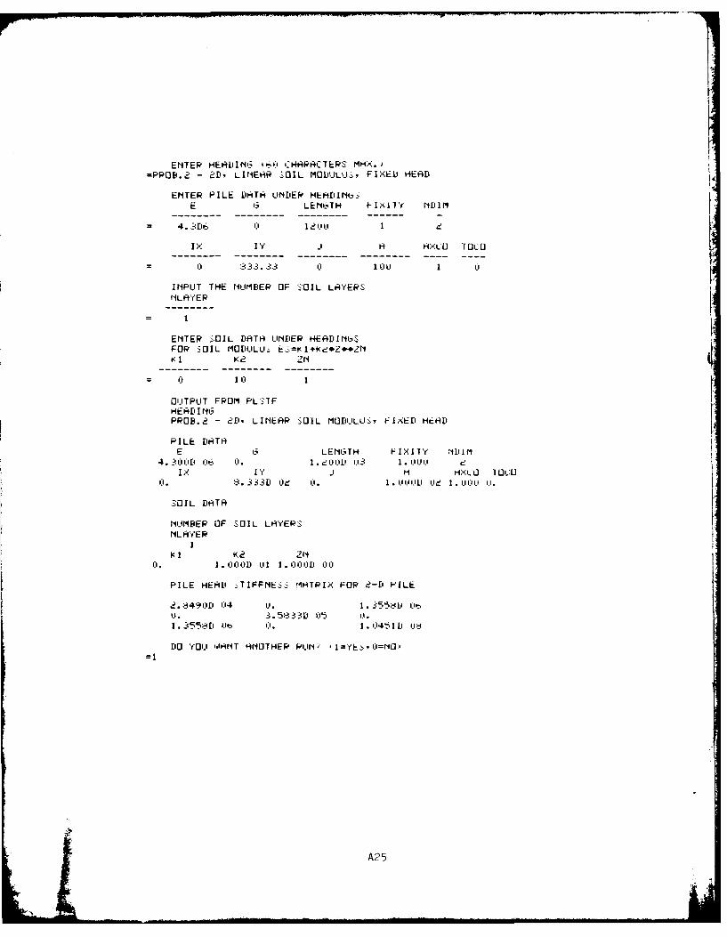
ENTER HERDING (66 CHHIRCTER:_ MHX.)=PROB.2 - 2D- LINEAR -,OIL MODULUS, FIXED HERD

ENTER PILE DHTA UrDER HERDINL,,.

E G LENbTH IxIy rILJlM

4. 3 D6 (I l2.U 1

IX I J H HXL:O TOC:O

03 3. 3 0 1 (ILI

I'PUT THE NUMBER OF ::OIL LAYERSNlLRYER

- I

ENTER SOIL DTA LIMNDER HEADLINb-:FOR SOIL MODULU ES=KI+l.e.ZnZNKI K.2 ZN

S10 1

OUTPUT FROM PL:§:TFHEADING

PROB.. - eD LINEAR SOIL MOD'ULUS', FIXED HEHD

PILE DHTHE T.LENGTH FIXITY rliM

4._3 0 0D 06 O. .dull. 1.1,3 1. lUll e'

IX IY J H HXLIO IOL:Ui. , 33

i'I (1. 1.1.UU i.LI 1. I IIII LI.

3IL DATA

N'UMBER OF .50lIL LAYERSNL AYE R

K1I K.2 ZN3. 1. 000D Ul 1. 000iiD 211:l

PILE HEAD .TIFFNESS"+ MHTRIX FOR d-D PILE

. 8491)D 14 .. 1. 355%df Vt,u. 3.5.334D 05 1).1.3558D ktp 0. 1. 0451D Qld

DO YOU IANT ANOTHER RU' 'I=YEz.. l=rO1,

A2 5

ENTER HERDING (60 CHARACTERS MAX.)=PROB. 2A - 2D, LINEAR SOIL MODULUS, 2 SOIL LAYERS

ENTER PILE DATA UNDER HEADINGSE 6 LENGTH FIXITY NDIM

4.3D6 0 1200 1 2

IX IY J A AXCO TOCO

0 833.33 0 100 1 0

INPUT THE NUMBER OF SOIL LAYERSNLAYER

= 2

ENTER SOIL DATA UNDER HEADINGSFOR SOIL MODULUS ES=KI+K2*Z*.ZNKI K2 ZN DEPTH GAMMA

--- 10 I 600 500 10 1 1200- 50

OUTPUT FROM PLSTFHEADINGPROB. 2A - 2D, LINEAR SOIL MODULUS, 2 SOIL LAYERS


4.300D 06 0. 1.200D 03 1.000 2IX IY J A AXCO TOCO

0. 8.333D 02 0. 1.000D 02 1.000 0.

:OIL DATA

NUMBER OF SOIL LAYERSNLRYER

2KK V2 ZN DEPTH GAMMA

0. 1.O00D 01 1.O0D 00 6.OOOD 02 5.00D 010. 1.O00D 01 1.000D 00 1.200D 03 5.OOOD 01

PILE HEAD STIFFNESS MATRIX FOR 2-D PILE

2.8490D 04 0. 1.3558D 060. 3.5833D 05 0.1.3558D 06 0. 1.0451D 08

DO YOU WANT ANOTHER RUN? (=YES,0=N0)=1

A26

ENTER HERDING (60 LHHR"LTER. 1 MHX.'=PROB. 3R - 2D cONST. "'S OFT" SOIL MOD.. HOT" PILE

ENTER PILE DATA Ur4DER HEHDING..

E G LENL'TH FI;ITY rii I M

1.5116 r0 360 0

Ix I," A R,_.O rl OGO

.-"0 . I.i6 063.5 I. U

INPUT THE NUMBER OF -SOIL LAYER:.rNLHYER

- 1

ENTER SOIL DATA UNDER HEADING--FOR :OIL MODULLI:S E=KI+K,*ZZ Nr; I K.2 ZiN

3.123

OUTPUT FROM PLSTFHEADINGPROB. 3A - 2D, CONST.'"SOFT" :SOIL MUD.. -HOWl. PILE

PILE DATA

E G, LENbIIH IxIAl'Y Nl'IM1.500:lD 06 0:l. -. 0,l1l 2i di.

IX IY _ 1! -L 0 1 LU 03.221D O O. 35 VD 1. bu. ki U.

-,OIL DATA

NUMBER OF SOIL LAYERSNL YER

e 1 K.2 ZN3. 1231' lil 0 . 0.

PILE HEAD STIFFNES.iS MATRIX FOR ,-1' PILE

2. -4 '15 U 0. 2 00. 1 .3229 (15 i.0. A. U.

Do YOU WI.ANT ANOTHER RULN I=YES.0=iML)=1

;' A27

i , ' "i

ENTER HEADING (_U CHHP'FiCTEP:-- M, -.. ,=PPOB. 3B - -FiME R- 3H EXCEPT "LONL," PILE

ENTER PILE DATA4 UNDER HEIDIIIN L,:E G LENGTH FIXITY NL I M

1 1 .5D6 0 1200 ' (

IX I ' HJ."L- O I UL .

S322.0 6.3.5 u. 5 u

INPUT THE NUMBEP OF 3OIL LH-rERS:*-NtLRYrER

ENTER :SOIL DHTF UINDER HENDIN _-FOR *SOZIL MODULUS ES=K1I+K.Zn,-NK I K2 Zt

=3.1 .3 00

OUTPLIT FROM PLS:TFHEADING;PROB. 3B - SA:ME HS 314 EXLEPT -LON,;- PILE

PILE DATAE I, LENl'TH FIXITY 1ILP1M

1.500D %, 0. 1. iUl, 13 ). dI X I J . HXC U TOCO

l. 3. L1I 0D i . t .. - l5 I ll 11 .t l.)ii l 1.

SOIL DITR

NUMBER OF S OIL LN'YER. S:NLAYER

I

KI K.2 ZN

3. 1231' 00 .. 0.

PILE HERD ]TIFFNESS:: MTRIX FOR e-D PILE

2.4t,31911 02 U. v0. 3. ' 1D 04 1.

[10 :OLl IAJHNT HrNOTHER WlrN 'I = CE-.O=U',=A

A28

i... . .. .. .

ENTER HERDING (LO CHRHCTERS MMX.)=PROB. C - SHME RS 3A EXCEPT LENGTH CALC. BY PROG.

ENTER PILE DATA UNDER HE-DII;'E G LENGTH FIXIfY ;IDUIM

- 1.5D6 0 0 1)

IX IY J A HXGO TOLD

0 3.22. 06 0 63.5 :1. 5 U

IN1PUT THE N'UMBER OF SOiL LH-Y'ER

rNLAYER

- I

ENTER S.OIL ['HTH UNDER HENDINL'oFOR SOIL MODULU.: ES=<1+ge2ZNKk 12 ZN

- 3.12 ',' 0

OUTPUT FROM PLS:TFHERDINMG

PROB. S.C - SA.RME RS 3H EXCEPT LENGTH CRLC. BY PROG.

PILE DATRE 0 LErtoTH FIX17Y rNDIM

1. 5001' 0 . I.b7D 03 u.IX IY J N HXCO I OLO

0. 3.221D 0. i.. e. 3501 l I.I l .11-

S:OIL DATA

NUMBER OF -OIL LAYERSNLRYER

1

K I K2 ZN3.12.3D 00 0. 0.

PILE HERD MFIFFNESS MATRIX FOR d-D PILE

2. 4-k48D 02 0.3. 11201 D U4 0.

DO YOU IRINT ANOTHER RUN'r? (1=YES,0l=NO)=1

A29

ENTER HERDING '0 L:HN4RiTER: MHX.)=PROB. 4 - SAME HS .3 EXCEPT STIFFER SOIL

ENTER PILE DRTR UNDER HEADING. :- E , LENGTH FIXITY NDIM

1.5D6 i 360 U

IX IY J H FiXLO 1 01.:U

0 322.06 0 b. 5 0.5

INPUT THE NUMBER OF :OIL LNYERSNLAY ER

- 1

ENTER SOIL DRTA UNDER HEAD INGSFOR SOIL MODULL ES=K+(. Z*,*,ZnNK I K2 ZN

- .31.2 00

OUTPUT FROM PLSTFHEAD I MGPROB. 4 - SAFRME AS .3 EX.EP1 STIFFER SOIL

PILE DATAE 6 LENGTH FIXITY NLuIM

1.5001D 06 Cf. 3. t0'1) I2 0.IX I Y H HXLU TOL:O

ci. 3.221 D ). U . L.31 i U.tAW u.

SOIL DATA

NUMBER OF :OIL LHYERSNLAYER

K I Ke ZN

3. 12 D 0-:i . Q.

PILE HEAD L..TIFFNES_, MRTRIX FOR e-L' PILE

1. 38401D 113 -l. II.0 •1. 3e 9[1 k1.

D1O YOU IRNT A4NOTHER RUW (I=YES.u O-N0'=1

A30

ENTER HEADING %t60 L:NRRtTERS MAX.)=PROB. 5 - SAME AS 3R AND 4 EXCEPT STIFFER A.:J]IL

ENTER PILE DmTR UNDER nbn-INbE C, LEtTH FIXITY NDIM

1.SDb 0 .u

IX IY J H HXL:O IuL:U

0 322.u6 ( 0 03.5 k.5 u

INPUT THE NUMBER OF SOIL LHYEISNL AYER

= 1

ENTER SOIL DATA UNDER -RDIN6S:FOR S01L MODULUS ES=K.+g.2*Z,,ZNK 1 K2 ZN

= 312.3 0 0

OUTPUT FROM PLSTFHEADINGPROB. 5 - SAME A:S ,3H HND 4 EXCEPT STIFFER SOIL

PILE DATAE , LENibi H FIXITY NDIM

1.500D 06 0. 3.tkulD O,12 0.

IX IY J N HXLO TOGOO. 3.221D 02 u. -,. D5 li L0. u u u u.

1SOIL DATA

NUMBER OF S:OIL LAYERSNLRYER

1

Kl WK2 ZN3. 123D 02Cf. .

PILE HEAD ::TIFFME:S3: MHTROIX FOR 2-11 PILE

7. 7913D 03 0. 0.

0. 1. 3229 1 05 .

DO YOU WHNT HNOTHER RUN, (I=YE .=N'J=1

A31

ENTER HEADING (60 CHARACTERS_ MHX..'=PRP. 6 -3D, LINEAR SOI0L MODULLL.' PINNED HEM])

ENTER PILE DAfTA UNDER NEA~IL'Nb.E c6 LENGTH FIXITY NIJIMh

- 4. 306 1. 8D6D i201_1 '3

9 3333. 3.33 1666.67 10'0

INPLIT THE NL'MBER OF AOIL LMYER_,NLnRYER

ENTER 'SOIL DATH UNDiER HEAHDIN,-FOR 3OIL MODULUS. E-K l+Kd*Z**ZN

OUTPLIT FROM PLSTFNEAD INGPROP. 6 - 3D. LINEAR S--OIL MODULUS'.i PINNED MENU1

PILE DATAE 13 LEN'LTH FIXIIlY N'DJM

4. 30'0' (' it;3 1 . 8t)('1' Ci36 1~ cll v 3'1 3 61.Ix IV J1 H HXL.O TOL'O

8. 333D 032 3S. 33It I'3 1 .tt:b7fD I"'3 1.ol'300k' 'ie 1.k:11 1. (' Li

SOIL DATA

NUMBER OF sOIL LAYERS,NLHrER

1K< I K 2211

03. 1 . 111) D '31 1 . IJ 1. U DL l V3

PILE HEAD z-TIFFNEES MATRIX r-OR ::-DF' ILE

I . f03 '31ID 04 uI. Cf. 0. 10.1.0(90~1 D (14I 0. Ll. Ll. L.

Cl. oJ. 3. V.. A' LS I

U.. 1..

0.. d.wvl 5J3' j

DO YOU IdMNT HNOTHERP19 (1YE. 3=10

A 32

ENTER HEADING (60 CHHRRC:TElS MAX.)=PROB. 7 - SAME AS 6 EXCEPT FIXED HER4D

ENTER PILE DATA UNDER HEADIN. :E G LENL'TH FIXITY NDIM

4.3D6 1.8D6 1200 1 3

Ix IY j H HXL:t IOLU

l8333.3.3 83 33 1666.67 101 1 1

INPUT THE NUMBER OF SOIL LAYERS,NLAYER

ENTER SOIL DATA UNDER HEADINC6:FOR SOIL MODULUS ES=g l+K82ZZN

Kl 1(8 ZN

1 1':' 1

OUTPUT FROM PLSTFHE DI NGPROB. 7 - SAME AS 6 EXCEPT FIXED HEAL

PILE DATA

E G LENGTH FIXITY NVIM4. 300D 06 1. .8001o (l 1. 00D (13 1.000 -

IX IlY J H HXLO TOLO:83.33D '02 8. 333D (38 1.&67D LiJ l. iuu L Lie l. UtU l.LJ

701L DATA

NUMBER OF SOIL LHYERSrILHYER

1

K I K.2 ZN1). 1. I::or'D 11 1 . 01.11 uUi.

PILE HEAD TIFFNES MATRIX FOR 3-1 PILE

.:. ;[email protected] 04 1, U. 0U. 1 , d55:.-I I l u.. 8. 84'0D 04 0. -1. 3-t55811 Lt, Ll. U U.

0. 3. 58-331' L15 0. U. U.

i. -1. s455811 it, I. 1.1451 [L .d L. Ll.1. 3-55:D 06 0. 0. V. 1. 045 ID 1I .1.

i. Co. Cf. U1.. 1. . .blLJUllU L t Ub

DO YOU WHNT HNO1THER Fo~rUN (I=rr-'y 0o110=A

A33

ENTER HEADIM6 (6t CHHPRLTER: MMX.)=PROB. 8 - SRME RS 7 EXCEPT PHPTIMLLY RESTPMINED HEHD

ENTER PILE DATA UNDER HERDIN.

E C, LENCGJH FIXITY MDlIM

4. 3 D6 1.s o 110u (1.5

IX IY j H HXL[I 1lL.U

833.33 33.33 166t.07 l00 I

INPUT THE NUMBER OF '.OIL LHYEO&

NLYER

= I

ENTER AOIL DHTR UNDER HEADIN.FOP SOIL MODULUL. ES=9(.i9e-.i..ZNKI K2 ZN

= 1 1

OUTPUT FROM PLSTFHERD I NGPROB. 8 - _RME HS 7 EXCEPT PRPTIALLY WESTNINED HEHD

PILE DRTA

E , LENGTH FIXITY NIJIM

4.300D 06 1.80OD 06 1. OuD 0.3 V,50-

IX I J A MXLO LO

8.3331' 02 H_.3331' 0 1.6beD 13 I.l0Ii 'i Ud . otol.I 1.1._11.

SOIL DATA

NUMBER OF SOIL LHYERSNLAYEP

1

K 1 K2 ZN

0. 1.D0001' 0 . 0001' 0O

PILE HERD _TIFFNESS MHTRIX FOP -4-D PILE

1.96,5D 04 0. ). 0. i.7791D U5 0.0. 1. 96951' 04 0. -6.7791D U5 u. 1.0. 0. 3.5833D 05 u. 0. 0.0. -6.7791D1 05 0. 5.e256D te V. V.

6.7791D 05 0. 0. 0). b. e5b ,' 0 .

0. ). ). o. U. d. 500.OL u

DO YOU WA-NT ANOTHER PUN, 1=YE ,u=NO)=1

A 314

. ... . .. .. . I l i I I I I I I .... . -- . . ... . . .. .. II ... . ... I .. ... .. .. . . . ' ' .. . ... ... ... ' "-I

ENTER HERDING (60 -H-4RACTERS MX..=PROB. 9 - SAME AS 7 EXL:EPT EXPONENTIAL SOIL MODULU,

ENTER PILE DATH UNDER HEHDINLE '3 LEMbTH F IXI TY ILlIM

4.3D-6 1.9116 12:0U 1

IX IY J H HAL.U IOLU

= 833.33 83 3. 33 1t66. b7 10u 1 1

INPUT THE NUMBER OF ,OIL LHYE'-sNLAYER

- I

ENTER S:OIL DfTA' UNDER HEH[LINo.FOR S OIL MODULUS ES=- l+le.Z*Z*NK I K.e ZN

OUTPUT FROM PLSTFHEADINGPROP. 9 - S:HME HS 7 EXCEPT EXPONENTIAL 'lIL MOLIULU,

PILE DATAE S LEIbYTH FIXIIY NiI IM

4.3(01 Oo 1.8 0m ut. 1.2 uD :3 1 .U .3I X ly J H HXLU 1OL.O

8. 333D 02 ;. 3331' u2 1.6L,7D 1L13 1. OUUD Lid 1. UUu 1. u

SOIL DRTA

NUMBER OF SOIL LAYER:SNLAYEP

1

K1 K 2 ZN0. 1..)(OD1 uil C.VUCD mu

PILE HEHD S:TIFFNESS MHTRIX FOR -C-D PILE

2. 0465D 05 0. 0. .5. '. ? I, U.0. 2. 0465D u5 u. -5. 3.27DI U, U.0. 0. 3. 583.iD 1U5 U. U.r. -5.3927D 06 0. 2.14-43D i8 . U.5. 3927D 1:16 0. U. 0. d.1433b U-1 U.0. 0. 0. 0. U. e.buUULIFI Ut

DO YOU WANT ANOTHER RUN' (1YkS, OU)SI

! A 35

ENTER HERDING (60 CHeRRl.:TERS MHX.,=PROB. 10 - 3D. DIFF. IX & IY, LINEHR SOIL MODULUS

ENTER PILE DHTA UNDER HEHINSE G LENGTH FIXITY NDI M

111. D6 2. 5D6 I-oO 1 3

IX IV J 14 HXL:OI 101:

1440 1000 2440 130 1 I

INPUT THE NUMBER OF SOIL LHYERS

rILAYER

= I

ENTER SOIL DATA UNDER HERDINGSFOR SOIL MODULUS ES=K.I+Kd*iNZ.,ZNK I K 2 Z11

160 32

OUTPUT FROM PLSTFHERDINGPROB. 10 - 3D, DIFF. IX & IYv LINELH SOIL MOTDULU

PILE DATAE G LENLIH FIXITY NL'IM

1.00D 07 2.500' 06 l. dOOeDI I 1. uut .IX IV j A HXLU TUt-U

1.4401 03 1 .GOO3ID 03 e.441'D 0 . ' L'e 1.1.11.10 1. 1 . 1i

SOIL DATA

NUMBER OF SOIL L4YERSNLRYER

Ki K2 ZN1.600D 01 3.200D1 i1 1.100D 0j

PILE HEAD STIFFNESS MATRIX FOP i-li PILE

.4239) (14 0. 0. 0. 4. 1 ID L V.i. 1. 018.1 48 05 (1. -5. 1 6531 ' ipb 0. U.'. 0l. 1. i1 .i1-I1D Vl 0. i.,0. -5. 1653 1D )6 L . 4. i,'JbD '.1d U.4. 161 7D 06 o. 0. 0. 3-. I4eIeD li iI.

i) 0. Ll. i.1 ,L. 5. iLI;l- CA I Lit:,

IO YOU WHNT NOTHER RUN-' (I=YE S(=NU)=A

ENTER HEADING *60 CHARACTERS MAX.)=PROB. 11 - SAME AS 9 EXCEPT 3 SOIL LAYER:--.*

ENTER PILE DATA UNDER HEADINGSE G LENGTH FIXITY NDIM

4.3D6 1.8D6 1200 1 3

IX IY i A AXCO TOCO

83:3.33 833.3:3 1666.67 100 1

INPUT THE NUMBER OF SOIL LAYERSNLRYEP

ENTER SOIL DATA UNDEP HEADINGSFOR SOIL MODULU- E-=1+k2.Z,,ZNP 1 K2 ZN DEPTH GAMMA

= 10 0 0 300 50= 10 0 0 600 40= 0 10 1 1200 50

OUTPdT FROM PLS;TFHEADINGPPOP. 11 - :RME AS 9 EXCEPT 3 SOIL LAYERS


4. 300D :16 1.800 1 06 1.200D 0:3 1.000 IX IY J A AXCO TOCO

S-,333D! 02 8,333D 02 1.,667D 03 1. OOOD 02 1. 000 1. 000

:SOIL DATA

NUMBER OF -OIL LAYERSNLAYEP

3l V2 ZN DEPTH GAMMA

1 OAAD '11 0. ). 3. 0001' 02 5. 00't (I1• r)(lD (| 0. 0 i. 6. O ri'i liP 4. IAllD Al

1.001'01 1. OOD 00 1.201D 0.3 5.000D11 (1

PILE HERD STIFFNES:S MRTPIX FOR 3-D PILE

1 4 0 17A. 1. 1, 1 D 05II. 1.9529' 0_ 0. -1,8'I f 5 ' , I,

0. 3.5*.3rD 05 0. 0.-1.89111D (5 0. 3.6 A."'

1, 5 , O. n, ~ O, .:', 5 Dr4 07

DO YOU. IIANT RNOTHER RLNll ,I=YEC',n

A -47 I- -

ENTER HERDING :60 CHARACTERS MAX.)=PROB. 12 - SAME A' 11 EXCEPT DIFF. SOIL PROPERTIES:

ENTER PILE DATA UNDER HEADINGSE G LENGTH FIXITY NDIM

4. :3D6 1. 8D6 1200 1 3

IxX IY J A A'CO TOCO

8.33.33 833.33 1666.67 100 1 1

INPUT THE NUMBER OF :SOIL LAYERSNLAYEP

ENTER SOIL DATA UNDER HEADINGSFOR '-OIL MODULLUE- ES=k 1+l2,Z**ZNvi V:2 ZN DEPTH GAMMA

= 10 0 0 :300 50= 0 10 1 600 40= : 10 2 1200 50

OUTPUT FROM PLSTFHEADINGPROB. 12 - SAME AE 11 EXCEPT DIFF. SOIL PROPERTIES


4.3001 06 1.801) 06 1.2001' 0:3 1.000 :3I' IY J A AXCO TOCO

:.3331' 112 8. :3:3:3D 02 1.667D 0:3 1.0001' ':2 1.000 1.000

-OIL [DATA

NUMBEP OF .OIL LAYERSzMLAYER

3P1 V2 ZN DEPTH GAMMA

1. I:':ri 01 0. I.1. (1.. jI. 02 5. ":'o:r' :1O. 1. :000D 1 1. O0(1(D 00 6.000D 02 4. O00'D 111

I . 'i:IiD '[1 2. ''':':r '0 1.200' (0, 5.0''D 01

PILE HEAD -TIFFNEI.C MATRIX FOP 3-D PILE

2.2'2 -'. 0-: .. 0. 2.40641, 05 1:.:. A.5 3-fD 0. - . 05 '1. IO.

I'. -2.4 1 '.1, 05 (1. 4. ' 5 ,I 07 Al.2.41'['41' 05 0. f.. '. 4.52Q-51 17 A.U . ,. * II. f. 0. 2.5: -11[111 06

DO 'YOU IANiT ANOTHER PUN 1 =E *=0

A-38

1 _ . .... i -.

APPENDIX B: USER'S GUIDE FOR PROGRAM FDRAW

General Introduction.

1. Documentation for the computer program FDRAW--an interactive

graphics post-processor--is presented in this appendix and includes a

general introduction, guide for data input, and example problems.

2. FDRAW is capable of displaying pile geometry, resultant axial

forces, several different pile loading factors, and elastic center dia-

grams. Program commands control the display. The program was developed

by Mr. John Jobst, St. Louis District.

3. FDRAW runs on the WES G-635, Macon H-6000, and Boeing CDC com-

puters in the time-sharing mode. It is limited to execution on a Tek- 4tronix 4014. The program is part of the CORPS library and is identified

by the program number X0036. To execute the program, issue one of the

following run commands. On the WES or Macon computer,

OLD WESLIB/CORPS/XO036,RGCS2Ddevice - TK4

On the Boeing computer,

OLD,CORPS/UN=CECELB

CALL,CORPS,X0036

4. Two bits of information are prompted for by the program before

any commands may be given:

a. The name of the plotting file created by an analysis run

of X0034.

b. The radius of the figures to be drawn on the screen (pilecoordinate units per inch of screen).

5. After this, any valid FDRAW command may be given. The program

assumes load case 1 to be the current load case until it is changed by

giving the "LOAD" command.

COMMANDS:

HELP To obtain a list of valid commands.

RADI To redefine the radius of the figures drawn on the screen(units that the coordinates of the Tiles are riven in perinch of screen).

LOAD To change the current load case.

GEOM To display pile locations, with the options of printingthe batter for each battered pile and/or numbering thepile.

COMB To display the combined bending factor for each pile andthe portion of that factor due solely to the axial loadon the pile, for the current load case.

C.BF. =Q3 + Q4 Q5FA -- + FB5

where Q3 = vertical load along U3 axis (kips)Q4 = moment about U1 axis (kip-ft)

Q4 = moment about U2 axis (kip-ft)

Q5 = moment about U 2axis (kip-ft)4

FA = allowable axial load (kips)

FB4 = allowable moment about minor principal axis(kip-ft)

FB5 = allowable moment about major principal axis(kip-ft)

PLF To display the pile load factor and P.L.F. Flag for eachpile for the current load case.

For pile in compression:

.L.F. = MAX {C.B.F.} P.L.F. Flag = BC}

For pile in tension:

P.L.F. = MAX {C.B.F.} P.L.F. Flag = BT}

AXFC To display the axial factor and P.L.F. Flag for eachpile for the current load case.

For pile in compression:

A.F. = Q ,CALOW

Where CALOW = Allowable Compressive Load (kips)For pile in tension:

A.F.B2TALOW

B2

where TALOW Allowable Tensile Load (kips)

FORCE To display the axial force, Q3, for each pile for thecurrent load case.

CCOMB Similar to "COMB" except that it displays the criticalcombined bending factor for all load cases and the criti-cal load case number, for each pile.

CPLF Similar to "PLF" except that it displays the critical

pile load factor for all load cases and the criticalload case number, for each pile.

CCAXFC Similar to "AXFC" except that it displays the criticalaxial factor for all load cases and the critical loadcase number, for all pile in compression.

CTAXFC To display everything "CCAXFC" does, except for all pile

in tension.

ELCEN To display the elastic center and resultant force diagramsfor all load cases.

END To end FDRAW.

Guide for Data Input

6. Program X0034 of the CORPS library creates a plotting file to

be used as the input data file for this program. Data are written to

this file according to the following guide. All input is in free field

(a comma or at least one blank should separate data items) except Group

5.Group 1 - Pile Data

A.1 LINENP

LINE = five digit line number

NP = total number of piles in the foundation

B. Note: Repeat NP (Number of Piles) number of times

LINE,U1,U2,U3,HANG 4Ul = distance from origin to pile along Ul-axis (feet)

U2 = distance from origin to pile along U2-axi7 (feet)

U3 = distance from origin to Pile along U3-axis (feet)

H = batter H vertical on 1 horizontal 0 -- vertical pile

ANG = clockwise angle between the positive U1 axis of thestructure and the Ul axis (direction of batter) of thepile (degrees)

'L B3

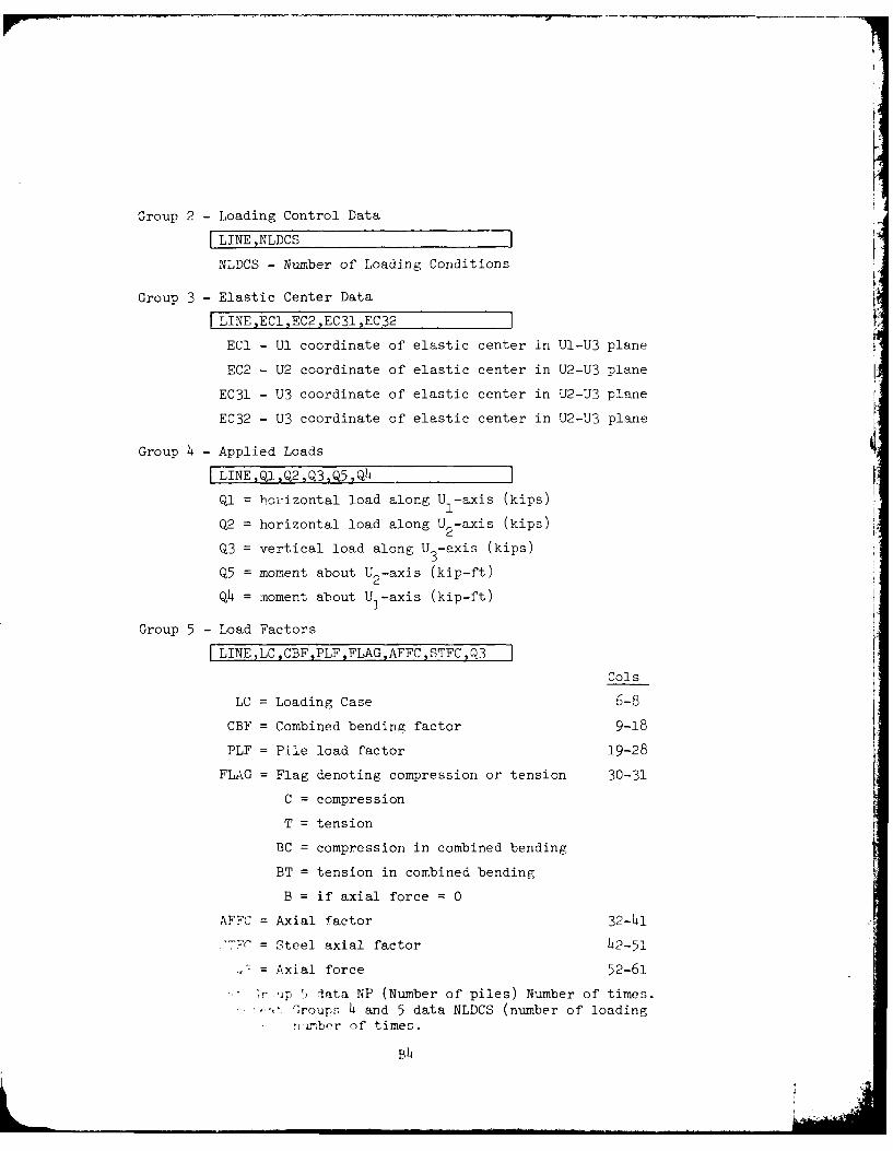
KGroup 2 - Loading Control Data

LINE,NLDCS

NLDCS - Number of Loading Conditions

Group 3 - Elastic Center Data

LINEEC1,EC2,EC31,EC32

ECI - U1 coordinate of elastic center in Ul-U3 plane

EC2 - U2 coordinate of elastic center in U2-U3 plane



Group 4 -Applied Loads

LINEQlQ2,Q3,Q5,Q4

Ql = horizontal load along U -axis (kips)1

Q2 = horizontal load along U2-axis (kips)

Q3 = vertical load along U -axis (kips)3

Q5 = moment about U -axis (kip-ft)2Q4 = moment about U 1-axis (kip-ft)

Group 5 -Load Factors

ILINELCCBFPLFFLAGAFFCSTFC,Q3

Cols

LC = Loading Case 6-8

CBF = Combined bending factor 9-18

PLF = Pile load factor 19-28

FLAG = Flag denoting compression or tension 30-31

C = compression

T = tension

BC = compression in combined bending

BT = tension in combined bending

B = if axial force = 0

AFFC = Axial factor 32-41

'7FC = Steel axial factor 42-51

= Axial force 52-61

r ip l data NP (Number of piles) Number of times.... . Groups h and 5 data NLDCS (number of loading

Snber of times.

B4

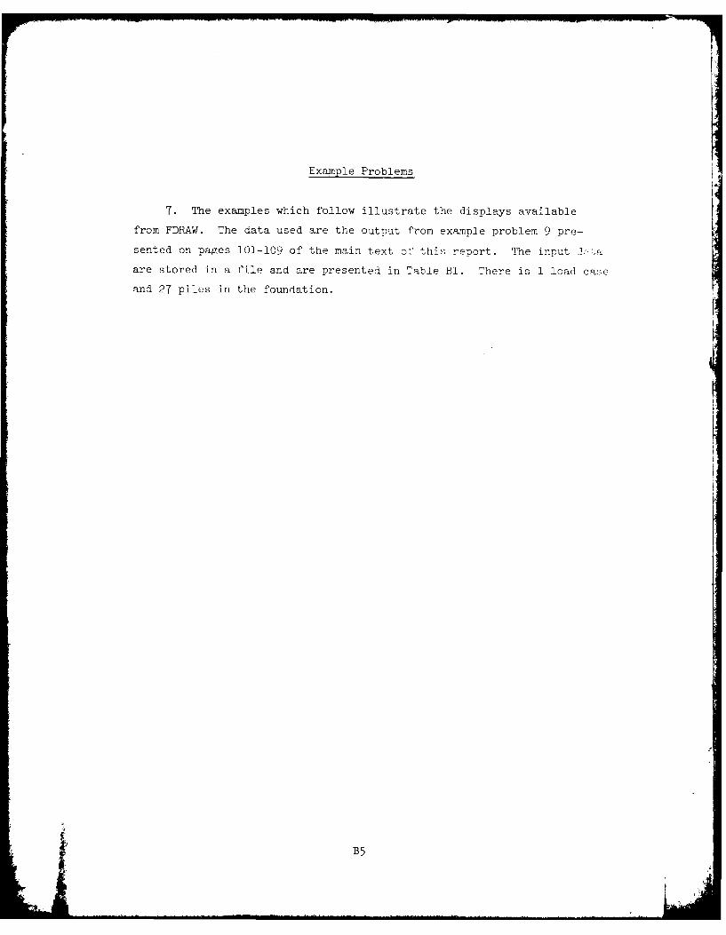
Example Problems

7. The examples which follow illustrate the displays available

from FDRAW. The data used are the output from example problem 9 pre-

sented on pages 101-109 of the main text of this report. The input J.ia

are stored in a file and are presented in Table Bl. There is 1 load case

and 27 piles in the foundation.

B5

afu

rH in

~*ff~.'fwY-v~ W-.-t

Q)e

!"4!4!*C*@*we ........

ewe...eee 0 O.*@ ............

- ---- -- ---- - - - - - - -

ill vz w2 st

- - - - - - - - - -- - - - - -- - - - - - - - - - - - - -.-

O.*@OOO [email protected]

THIS PASS0000.wmwwl"OO

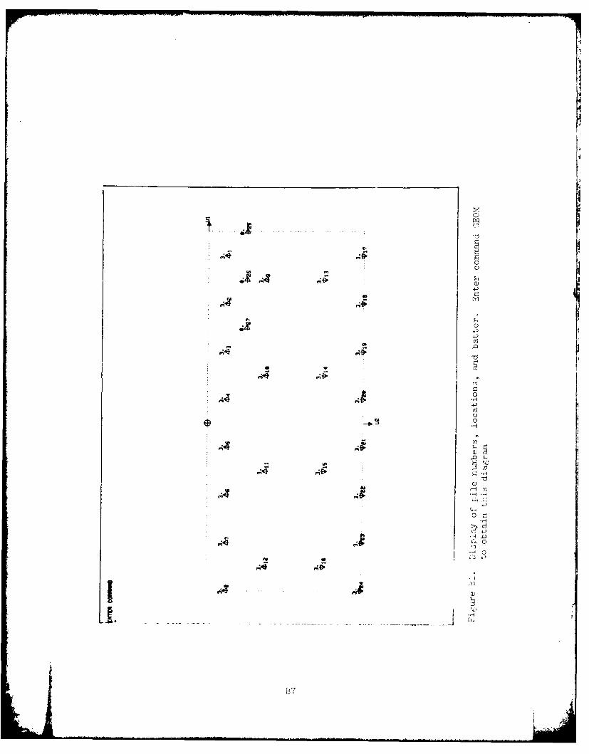
I

0

00

w I,

C)4-)

U 0

C)4-'4-'

0

0

g 0

4-'

U

W 0

HU)

~C)

01H '-4

-z4-'

00

I- H ,Df44

flu *0 *H 0

'-4

0 z C)

e.;~* -I. -* __ I

r~.

BY

C14-

o ::

4-'

C) CU

Mu 04 4-)

A d rf

4-' r

C) cCdj

0c

.4-

ZCU AC0 4-) +

. X- 0 t

-)

ll

A& C

0

1 0~

400

r,

0

4-

0

42C. r

0 a)

-i a)

0

4),)

H

O'd

ci0

13100

.q 0d

dU)

(y) 4-'

0); 0

0 Nq

c-z

0 1

474

e16C

Cd c

0 -M : vco C)0

cd H

qud

00

C)

H

0

0

-) 4- '

0n

BL-)U

~C) Q

-Cd

C)

H4-

+) 0

0 4-

0 r_

4-) 0

0

B13!

~~ -c - ---

0)

H I

0

4C

OU

4d CJci

H 4

B1

4--jb

U 4-)

4a

ft x

+)o

o 4-

4 ~0-

od C:~

: % o

-4-)

04-

04-)

Ct o,-

a1)EUU

Ct,. Hcd H4

H C-

001

WH Cd -

S- 0 I.D

r4) H 0

B] 5

°,'.4

4-)~

Q)0

4-~)

- u

C)O

Q)

Q) ( H

Q)

4,4

o)

to)

B16u I

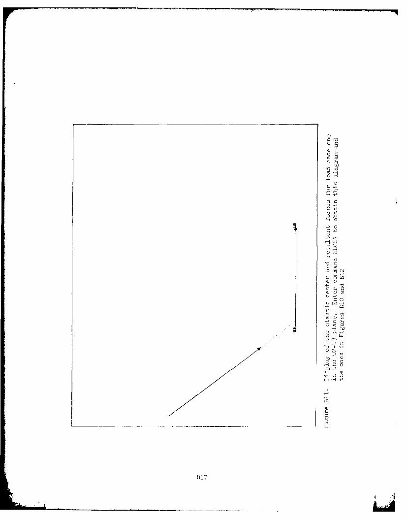
Cd

0 rd

0

in

C)d

00C 0

40

4-) 7

r-Cjd

1) '5

0 N

z0

4)i-P U

z)A

4)317~

7 AD-A087 191 ARMY ENGINEER WATERWAYS EXPERIMENT STATION VICKSBURG MS F/B 13/13

JUN 80 D K MARTIN, H W JONES, N RAOHAERISHNANUNCLASSIFIED WES-YR-K-AG 3 NL

00 0A

+d w Q

~ 43

z pq

a) 0. r. r-ad

B10

rA~

In accordance with letter from DAEN-RDC, DAEN-ASI dated22 July 1977, Subject: Facsimile Catalog Cards forLaboratory Technical Publications, a facsimile catalogcard in Library of Congress MARC format is reproducedbelow.

Martin, Deborah KDocumentation for LMVDPILE program / by Deborah K. Martin,

H. Wayne Jones, N. Radhakrishnan. Vicksburg, Miss. :U. S. Waterways Experiment Station ; Springfield, Va.available from National Technical Information Service, 1980.

132, 38, 18 p. : ill. ; 27 cm. (Technical report - U. S.Army Enginecr Waterways Experiment Station ; K-80-3)

Prepared for U. S. Army Engineer Division, Lower Missis-sippi Valley, Vicksburg, Miss.References: p. 132.

1. Computer programs. 2. Computerized simulation. 3. Docu-mentation. 4. Matrix analysis. 4. LMVDPILE (Computer program).S. Pile caps. 6. Pile foundations. I. Jones, H. Wayne, jointauthor. II. Radhakrishnan, Narayanswamy, joint author.TIT. United States. Army. Corps of Engineers. Lower MississippiValley Division. IV. Series: United States. Waterways Experi-ment Station, Vicksburg, Miss. Technical report ; K-80-3.TA7.W34 no.K-80-3

: ... .... .... ... ... .... F ... . I . ..... . . .. . . .. .. . ... .. . ... .. ... ... . . .. .IIII . .. . .... I~l ll . .. .. .. .. I I1| .. .. ... ... ... .. ...

eeee',e - defense technical information center · sor routine called pilestf that can compute...

Documents