e&f chaos: a user friendly software package for nonlinear...

Comput Econ (2008) 32:221–244DOI 10.1007/s10614-008-9130-x

E&F Chaos: A User Friendly Software Packagefor Nonlinear Economic Dynamics

Cees Diks · Cars Hommes · Valentyn Panchenko ·Roy van der Weide

Accepted: 27 March 2008 / Published online: 22 April 2008© The Author(s) 2008

Abstract The use of nonlinear dynamic models in economics and finance hasexpanded rapidly in the last two decades. Numerical simulation is crucial in the investi-gation of nonlinear systems.E&FChaos is an easy-to-use and freely available softwarepackage for simulation of nonlinear dynamic models to investigate stability of steadystates and the presence of periodic orbits and chaos by standard numerical simulationtechniques such as time series, phase plots, bifurcation diagrams, Lyapunov exponentplots, basin boundary plots and graphical analysis. The package contains many well-known nonlinear models, including applications in economics and finance, and is easyto use for non-specialists. New models and extensions or variations are easy to imple-ment within the software package without the use of a compiler or other software.The software is demonstrated by investigating the dynamical behavior of some simpleexamples of the familiar cobweb model, including an extension with heterogeneousagents and asynchronous updating of strategies. Simulations with the E&F Chaossoftware quickly provide information about local and global dynamics and easily leadto challenging questions for further mathematical analysis.

C. Diks (B) · C. HommesCeNDEF, Department of Quantitative Economics, University of Amsterdam,Roetersstraat 11, 1018 WB Amsterdam, the Netherlandse-mail: [email protected]

C. Hommese-mail: [email protected]

V. PanchenkoSchool of Economics, University of New South Wales, Sydney, NSW, 2052, Australiae-mail: [email protected]

R. van der WeideThe World Bank, Washington, DC, USAe-mail: [email protected]

123

222 C. Diks et al.

Keywords Nonlinear dynamics · Simulation software · Heterogeneous agents

JEL Classification C60 · E37 · G10

1 Introduction

In the last two decades the theory of nonlinear dynamical systems has flourished, anda wide range of mathematical tools for the analysis of nonlinear differential equa-tions as well as nonlinear maps have become available, see e.g. textbook treatmentssuch as Guckenheimer and Holmes (1983), Grandmont (1988), Arrowsmith and Place(1995),Mira et al. (1996), andMedio andLines (2001). Nonlinear dynamics tools havebeen widely applied in economics and finance, among others, through the work ofGrandmont (1985), Boldrin and Woodford (1990), Brock et al. (1991), Hommes(1991), Medio (1992), Day (1994) and Rosser (2000). More recently, the boundedrationality and interacting agents approach in economics and finance provides a naturalframework to modeling markets as nonlinear, adaptive systems, see e.g. the surveys ofHommes (2006) and LeBaron (2006). Since nonlinear dynamical systems are difficultto solve analytically, numerical analysis and simulations play a key role in the analysisof nonlinear systems and its applications.The purpose of this paper is to discuss the main features of theE&FChaos software

package with a menu-driven interface for simulation of nonlinear dynamical systems.“E&F” stands for Economics and Finance, because the package contains a list ofbenchmark applications in economics and finance. Many researchers and specialistsin the field have developed their own software for advanced numerical analysis of non-linear systems. But specialized software is not always easy to use. E&F Chaos is easyto use since it has been developed for use by non-specialists, students and researchersin economics and finance who would like a quick start in applying standard simu-lation tools for nonlinear dynamic models. The software program and source codeare freely available at http://www.feb.uva.nl/cendef and the numerical accuracy andquality of graphics allow direct generation of publication quality output for teachingand research. A convenient feature of the package is that new models can easily beincluded as a text file, without the need of a compiler or additional software. Once anew model has been included, basic tools such as time series, phase plots, bifurca-tion diagrams and largest Lyapunov exponents plots become immediately available.Simulation with E&F Chaos easily leads to challenging mathematical and economicquestions for further analysis.The paper is organized as follows. Section 2 gives some background informa-

tion about the development of the E&F Chaos program and briefly discusses somerelated software packages. The most important features of E&F Chaos are illus-trated through simulation of economic examples in Sects. 3 and 4. Although thesoftware does include a number of nonlinear differential equation models, we restrictour attention here to nonlinear difference equations, since most nonlinear applica-tions in economics are in discrete time. Section 3 considers an example of a one-dimensional (1-D) model, the cobweb model with adaptive expectations, whereasSect. 4 considers an example of a higher dimensional (4-D) model, the cobweb

123

E&F Chaos: A Software Package for Nonlinear Economic Dynamics 223

model with heterogeneous expectations. This section considers an extension of thecobweb model with heterogeneous expectation rules of Brock and Hommes (1997),to allow for asynchronous updating of strategies. The E&F Chaos software is used toinvestigate how asynchronous updating affects the dynamical behavior. Both Sects. 3and 4 are subdivided into subsections illustrating the key features, in particular theoptions from the Plot menu, of the software. The paper ends with a short concludingsection.

2 About E&F Chaos and Related Software

The earliest version of the E&F Chaos software dates back to the early nineties,when a DOS version programmed in Turbo Pascal was used in teaching of courses indynamical systems and nonlinear economic dynamics, both at the advanced bache-lor and themasters level, at the economics department of theUniversity ofAmsterdam.At the end of the nineties, a major revision of the software took place and aWindows version with a graphical user interface was developed. Both the user inter-face and the core routines for all calculations were programmed in Delphi 4.0.1 Thisversion has been around essentially unmodified since 1998, and was used in teachingthe aforementioned courses as well as NAKE Ph.D courses on nonlinear economicdynamics attended by Ph.D students from all Dutch faculties of economics. Orig-inally all (economic) models were hard-coded in Delphi Pascal. The advantage ofusing a low-level programming language was the speed of the resulting executablecode, which could easily exceed that of more flexible interpreted languages (Basic,Mathematica) by a factor of 10–100. This was important for computationally inten-sive algorithms, such as creating bifurcation diagrams or determining basin bound-aries of attractors. However, a clear disadvantage was that for every new model thesource code had to be extended after which the program needed to be re-compiled.In practice this meant that it was not straightforward for students to analyze a newmodel independently. They either needed to wait for implementation of the particu-lar model by the developers, or develop and compile parts of new code themselves.As a result, the old version was rather inflexible, and the number of ‘hard-wired’models appearing in the program’s menu started to grow, apparently beyond anybounds.In this paper we give an overview of the functionality and implementation of the

latest version of the E&F Chaos package as of June 2007. With the advent of tech-niques such as just-in-time compilation, scripting languages became available withthe flexibility of low-level code such as Pascal or C, while their speed is comparableto that of compiled code. This allows one to specify the model code in such a scriptinglanguage, and skip the cumbersome compilation step, practically without any loss ofspeed. Since each model can then be specified in a text file that can be interpreted ‘onthe fly’ one may simply work with a model by loading it, so that the long menus canbe dispensed of easily. We have chosen for the open source scripting language LUA as

1 We are indebted to Remco Peters, who, together with Roy van der Weide, programmed the initial Delphicode.

123

224 C. Diks et al.

it allows high flexibility as well as speed. A second recent addition is the replacementof bitmap graphics by high-quality Encapsulated Postscript (EPS) figures. To this endwe use the gnuplot program (see Racine 2006). To prevent the user from having todownload and install gnuplot separately, and to avoid possible incompatibilities withfuture versions of gnuplot, we have chosen to distribute the necessary gnuplot fileswith E&F Chaos.

2.1 Comparison with Existing Software

Many packages are available for the simulation and analysis of dynamical systems.Since it is beyond the scope of this paper to review all of them, we refer the inter-ested reader to the dynamical systems web portal at http://www.dynamicalsystems.org/sw/sw/, where users can choose their preferred package that best matches theircomputational needs. One can distinguish many different types of simulation soft-ware. Several dynamical systems software packages are implemented as toolboxesfor multi-purpose high-level programming environments such as Matlab, Octave,S-Plus or R. These environments are suitable for simulating a single or a few timeseries and generating high-level graphical output, for instance of phase plots of theattractors. For more computationally intensive graphs, such as bifurcation diagramsor basin boundaries, a lower level compiler-based programming environment such asPascal or C is more suitable. There are also several software packages available formore advanced numerical analysis, such as computing stable and unstable manifoldsand computing bifurcation curves (so-called continuation software). Examples areDynamics 2 (Nusse and Yorke), DSTool (Guckenheimer, a.o.), Auto2000 (Doedelet al. 2001) and Content (Kuznetsov). Some of the numerical procedures used in thesesoftware packages are based on advanced mathematical results concerning numeri-cal detection of manifolds (e.g. Nusse and Yorke 1998) and bifurcation curves (e.g.Kuznetsov 1995).The E&FChaos program is a stand-aloneWindows software package for the initial

numerical exploration of dynamical systems formulated by students or researchers.In terms of functionality and implementation, E&F Chaos is perhaps most closelyrelated to the iDMC package developed by the universities of Udine and Ca’Foscariof Venice as part of a teaching unit, which also includes a textbook containing manyexamples and exercises (Medio and Lines 2001). Both iDMC andE&FChaos simulatedynamical systems using the LUA language, inwhich the user specifies themodel. Thegraphical user interface of iDMC is implemented in Java, which has the advantage ofbeing platform independent (a Windows as well as a Linux version are available), butthe user has to install the Java Runtime Environment as well.2 E&F Chaos and iDMCshare many functional features, but differ in the way the user specifies the details andthe way in which the results are presented.

E&FChaos provides the user with default choices for the parameters to be specifiedfor each of the methods, endorsing the philosophy to provide a quick initial analysisof the dynamics of a specified model. To include a new model for simulations, the

2 E&F Chaos can be run under the Wine translation layer on Linux systems.

123


user only has to specify the dynamics in the flexible LUA language, as a text file.If desired, auxilary variables for which output (e.g. a time series) is required can bedefined and included in the specification. Prior analytic calculations, such as com-putation of a Jacobian matrix, are not necessary. For example, in order to computethe largest Lyapunov exponent E&F Chaos evaluates the Jacobian numerically fromthe specified map, rather than from an analytic expression of the Jacobian matrix;see Subsect. 4.5 for more details. To allow further processing of the data generated,E&F Chaos allows the data represented in any graph to be written to file in plaintext format. E&F Chaos provides graphical output in a range of formats, includingbitmap, Windows Metafile and Enhanced Metafile. It is possible to generate publica-tion quality output of graphs aswell, inwhich case gnuplotwill be called to generate anEncapsulated Postscript (.EPS) file. To keep the style and details such as axes labelsof these high-quality graphs flexible, there is an option to save the gnuplot file aswell as a data file in plain text format, which can be edited and processed by gnuplotlater if desired. All figures in the current paper have been directly generated by E&FChaos.3

3 One-Dimensional Example

To illustrate simulation of a 1-D system, we consider a simple economic example, thecobweb model with adaptive expectations. The classical cobweb model is a partialequilibrium model describing price fluctuations of a non-storable consumption good.There is a one period lag in production, so producers have to form price expectationsone period ahead. Demand, supply and market clearing are given by

D(pt ) = a − dpt , a ∈ R, d ≥ 0 (1)

Sλ(pet ) = arctan(λpet ), λ > 0, (2)

D(pt ) = Sλ(pet ). (3)

Demand D is a linearly decreasing function in the market price pt , with slope −b.Following Chiarella (1988) and Hommes (1994), we consider a nonlinear, increasing,S-shaped supply curve Sλ, where the parameter λ tunes the nonlinearity of the supplycurve.4To close the model we have to specify how producers form price expectations. The

simplest case, studied in the thirties e.g. by Ezekiel (1938), assumes that producers

3 Encapsulated Postscript (EPS) files can be viewed and processed by many software packages, suchas Ghostview (http://pages.cs.wisc.edu/ghost/), GNU gv (http://www.gnu.org/software/gv/), and can beimported by document typesetting software such as LaTeX.4 We use the same specification as in Hommes (1994), with the inflection point of the supply curve chosenas the origin. Negative values thus mean negative deviations from this inflection point.

123

226 C. Diks et al.

have naive expectations, that is, their prediction equals the last observed price pet =pt−1. In his seminal paper Muth (1961) used the framework of the cobweb modelto introduce rational expectations, with the price forecast pe = p∗, where p∗ is theprice corresponding to the intersection point of demand and supply. Here we considerthe case of adaptive expectations, proposed by Nerlove (1958). In contrast to Nerlove(1958), we have a non-linear, instead of a linear, supply curve. Adaptive expectationsare given by

pet = (1− w)pet−1 + wpt−1, 0 ≤ w ≤ 1, (4)

wherew is the expectations weight factor. The expected price is a weighted average ofyesterday’s expected and realized prices, or equivalently, the expected price is adaptedby a factor w in the direction of the most recent realization. A simple computation,using (1–3) and (4), shows that the dynamics of expected prices becomes

pet = (1− w)pet−1 + wa − arctan(λpet−1)

b= fw,a,b,λ(p

et−1). (5)

Dynamics of (expected) prices in the cobweb model with adaptive expectations isthus given by a 1-D system xt = fw,a,b,λ(xt−1) with four model parameters. We nextdiscuss how this model can be simulated in E&F Chaos.

3.1 Getting Started with E&F Chaos

After installing the software packageE&FChaos two directories are created: ‘gnuplot’(containing all gnuplot files) and ‘Models’ (containing all model files). The modelsare collected in three subdirectories, ‘Continuous’ and ‘Discrete’ (containing somebenchmark examples of nonlinear differential and difference equations, respectively),and ‘My Models’, containing newly created models by the user. When running thesoftware, the E&F Chaoswindow appears, with an easy-to-use Windows menu struc-ture. To simulate the model of this section, the user can use the File/LoadModel menu,open the subdirectory ‘My Models’ and select the file ‘Cobweb Adaptive Expecta-tions’ to run simulations. All menu/submenu items are also available as panel buttonsat the top of the E&F Chaos window.

3.2 Time Series

The most important menu in the E&F Chaos software is the Plot menu, where allgraphical plot submenus are collected, which will be illustrated throughout this paper.Chiarella (1988) and Hommes (1991, 1994) have shown that the cobweb model with alinear demand curve and a nonlinear, butmonotonic, supply curve can generate chaoticfluctuations. Using the Time Series submenu, an example of a chaotic price series isillustrated in Fig. 1. Each graphical window, such as the ‘Time Series’ window, has asubmenu ‘Edit’, which enables the user to change parameter values, the initial state,the plot variable (only the expected price ‘x’ in this example), the number of points

123


0 0.5

1 1.5

2 2.5

3

0 20 40 60 80 100

xt

time

-2

-1

0

1

2

3

4

5

-2 -1 0 1 2 3 4 5

f(x)

x

Fig. 1 Chaotic time series (left panel) for expectations weight factorw = 0.5, with other parameter valuesλ = 4.4, a = 1 and b = 0.25 and initial state x0 = 0.3. A graphical analysis (right panel) shows that themap fw,a,b,λ is non-monotonic with two critical points, with a maximum and a minimum, and that initialstate x0 = 0.3 does not converge to a low periodic orbit

plotted, the number of points not plotted (so that a transient phase can be skipped) andthe time step (so that e.g. each 10th period can be plotted). The Time Series menu hasthe additional option ‘Connect Points’ (if on, then points are connected by a line) and‘Plot Squares’ (if on, then each point is represented by a square). Scaling can be doneeither automatically (default) or manually.

3.3 Graphical Analysis

One-dimensional (1-D) systems xt = f (xt−1) are relatively easy to analyze, since thegraph of the corresponding 1-D generating map f essentially determines the dynami-cal behavior. The Graphical Analysis submenu (only available for 1-D systems) givesthe possibility for detailed investigations of the graph of the map f and higher orderiterates f k , k ≥ 2 (i.e. applying the map f k times). Figure1 (right panel) shows thatthe graph of the map fw,a,b,λ in (5) is a non-monotonic map, with two critical pointswhere the graph has a (local) maximum and a (local) minimum, respectively. In theSettings submenu, the user can specify the range of the interval (i.e. minimum andmaximum), the number of iterates and an initial state. By clicking ‘Next Iteration(s)’the next steps in the graphical analysis (i.e. a horizontal line segment connecting thelast point to the diagonal y = x , and a vertical line segment connecting this point tothe graph of the map) appear. By repeatedly clicking ‘Next Iteration(s)’ a ‘cobwebdiagram’ as in Fig. 1 (right panel) appears, illustrating the dynamical behavior. Sincethe graphical analysis in this example does not converge, it suggests that the dynam-ical behavior is chaotic. After clicking ‘Clear Form’, the graphical analysis can berepeated. Using the Edit submenu, the user can specify the number of time steps asan integer k (so that one click to ‘Next Iteration(s)’ yields k steps in the graphicalanalysis). In Subsect. 3.6 we will return to the ‘Graphical Analysis’ to investigatebifurcations in this model.

123

228 C. Diks et al.

3.4 Bifurcation Diagram

A powerful tool for investigating how the dynamical behavior of a nonlinear modeldepends on a single parameter is a bifurcation diagram. A bifurcation is a quali-tative change in the dynamics as a model parameter changes. For instance, a fixedpoint becomes unstable if one or more eigenvalues of the linearized dynamics aroundthe fixed point cross the unit circle. The three possible scenarios in which that mayhappen are (see e.g. Kuznetsov 1995 for a mathematical treatment of bifurcationtheory):• an eigenvalue λ = +1: typically this corresponds to a saddle node or tangentbifurcation from 0 to 2 steady states. Other possibilities are a pitchfork bifurcation(from 1 to 3 steady states) or a transcritical bifurcation (exchange of stability of 2steady states);

• an eigenvalue λ = −1: period doubling or flip bifurcation, with creation of a2-cycle;

• a complex pair of eigenvalues with ‖λ‖ = 1: Hopf or Neimark–Sacker bifurcation.This possibility only arises for two or higher dimensional systems.

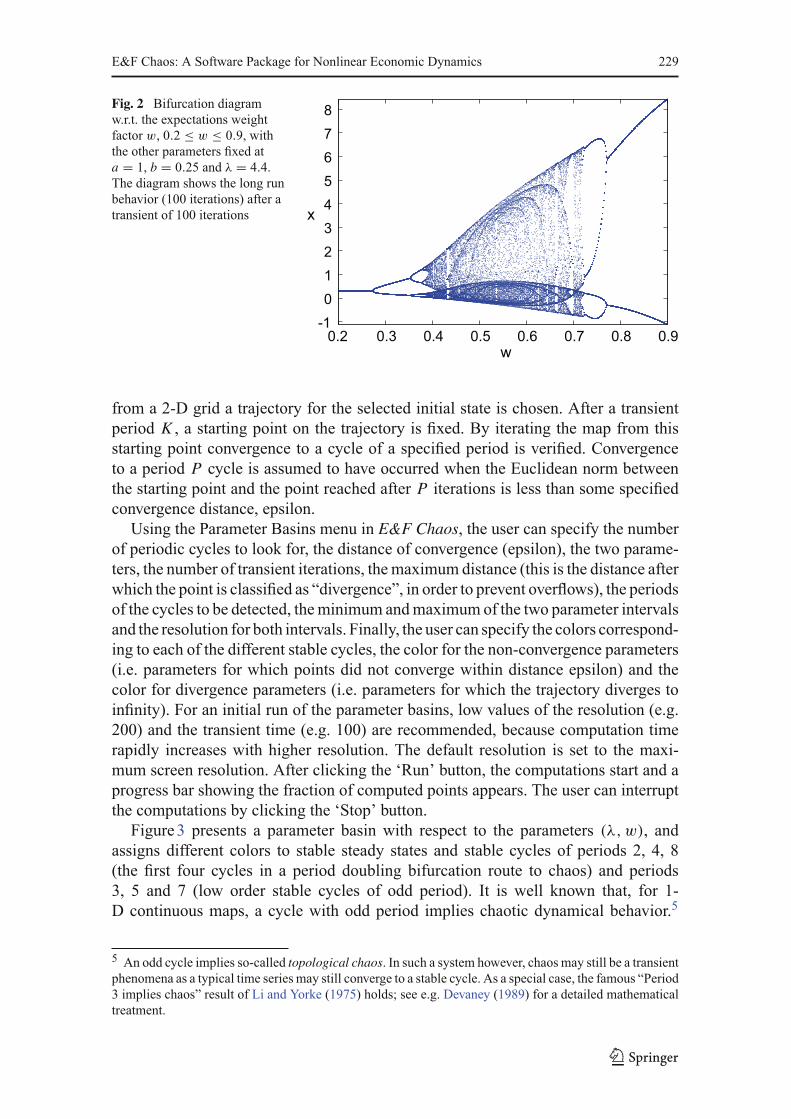
A bifurcation diagram shows the long run dynamical behavior as a function of a modelparameter. After selecting the Bifurcation Diagram menu, the user can specify (or usethe default values) the parameter, its minimum and maximum value, the plot variable,the number of points to be plotted and the transient time (i.e. the number of pointsskipped before plotting is started). To provide different ways of dealing with the pos-sibility of multiple attractors, there are several options for the initial conditions fordifferent parameter values as the bifurcation diagram is computed. There are threeoptions: (i; default option) initialize on the same, fixed initial condition for each newparameter value, (ii) initialize on the last point plotted for the previous, slightly smallerparameter value, (iii) compute the diagram from ‘right to left’, i.e. from high to lowvalues, with initial states as in (i) or (ii). Options (ii) and (iii) are intended to keepthe orbit on the ‘same’ attractor as the parameter slowly changes, thus following theattractor as long as it exists.Figure2 shows a bifurcation diagram of the cobweb model with adaptive expec-

tations with respect to the expectations weight factor w, illustrating the long rundynamics (100 iterations) after omitting a transient phase of 100 iterations. For smallvalues of w, 0≤ w ≤ 0.27, prices converge to a stable steady state, while for highvalues ofw, 0.77 < w ≤ 1 (close to naive expectations) prices converge to a stable 2-cycle with large amplitude. For intermediatew-values however, say for 0.4< w < 0.7,chaotic price oscillations of moderate amplitude arise. In particular, the chaotic pricefluctuations for w = 0.5 have been illustrated already in Fig. 1.

3.5 Parameter Basins

An even more powerful tool in the numerical analysis of nonlinear dynamics are theParameter Basin plots, sometimes also called 2-D bifurcation diagrams. A parameterbasin plot assigns different colors in a 2-D parameter space to stable cycles of differentperiods. The parameter basins are computed as follows. For the selected parameters

123


Fig. 2 Bifurcation diagramw.r.t. the expectations weightfactor w, 0.2 ≤ w ≤ 0.9, withthe other parameters fixed ata = 1, b = 0.25 and λ = 4.4.The diagram shows the long runbehavior (100 iterations) after atransient of 100 iterations

-1012345678

0.2 0.3 0.4 0.5 0.6 0.7 0.8 0.9

x

w

from a 2-D grid a trajectory for the selected initial state is chosen. After a transientperiod K , a starting point on the trajectory is fixed. By iterating the map from thisstarting point convergence to a cycle of a specified period is verified. Convergenceto a period P cycle is assumed to have occurred when the Euclidean norm betweenthe starting point and the point reached after P iterations is less than some specifiedconvergence distance, epsilon.Using the Parameter Basins menu in E&F Chaos, the user can specify the number

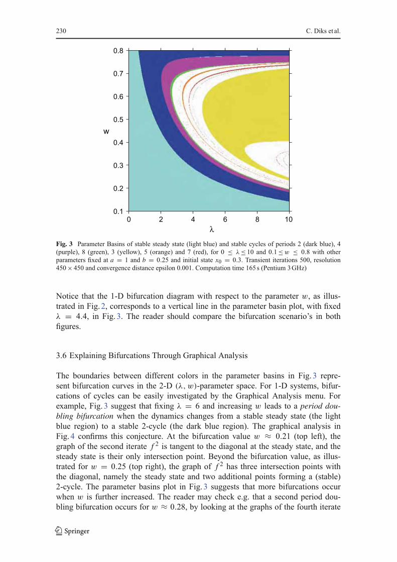
of periodic cycles to look for, the distance of convergence (epsilon), the two parame-ters, the number of transient iterations, themaximum distance (this is the distance afterwhich the point is classified as “divergence”, in order to prevent overflows), the periodsof the cycles to be detected, theminimum andmaximum of the two parameter intervalsand the resolution for both intervals. Finally, the user can specify the colors correspond-ing to each of the different stable cycles, the color for the non-convergence parameters(i.e. parameters for which points did not converge within distance epsilon) and thecolor for divergence parameters (i.e. parameters for which the trajectory diverges toinfinity). For an initial run of the parameter basins, low values of the resolution (e.g.200) and the transient time (e.g. 100) are recommended, because computation timerapidly increases with higher resolution. The default resolution is set to the maxi-mum screen resolution. After clicking the ‘Run’ button, the computations start and aprogress bar showing the fraction of computed points appears. The user can interruptthe computations by clicking the ‘Stop’ button.Figure3 presents a parameter basin with respect to the parameters (λ,w), and

assigns different colors to stable steady states and stable cycles of periods 2, 4, 8(the first four cycles in a period doubling bifurcation route to chaos) and periods3, 5 and 7 (low order stable cycles of odd period). It is well known that, for 1-D continuous maps, a cycle with odd period implies chaotic dynamical behavior.5

5 An odd cycle implies so-called topological chaos. In such a system however, chaos may still be a transientphenomena as a typical time series may still converge to a stable cycle. As a special case, the famous “Period3 implies chaos” result of Li and Yorke (1975) holds; see e.g. Devaney (1989) for a detailed mathematicaltreatment.

123

230 C. Diks et al.

0.1

0.2

0.3

0.4

0.5

0.6

0.7

0.8

0 2 4 6 8 10

w

λ

Fig. 3 Parameter Basins of stable steady state (light blue) and stable cycles of periods 2 (dark blue), 4(purple), 8 (green), 3 (yellow), 5 (orange) and 7 (red), for 0 ≤ λ ≤ 10 and 0.1≤w ≤ 0.8 with otherparameters fixed at a = 1 and b = 0.25 and initial state x0 = 0.3. Transient iterations 500, resolution450× 450 and convergence distance epsilon 0.001. Computation time 165s (Pentium 3GHz)

Notice that the 1-D bifurcation diagram with respect to the parameter w, as illus-trated in Fig. 2, corresponds to a vertical line in the parameter basin plot, with fixedλ = 4.4, in Fig. 3. The reader should compare the bifurcation scenario’s in bothfigures.

3.6 Explaining Bifurcations Through Graphical Analysis

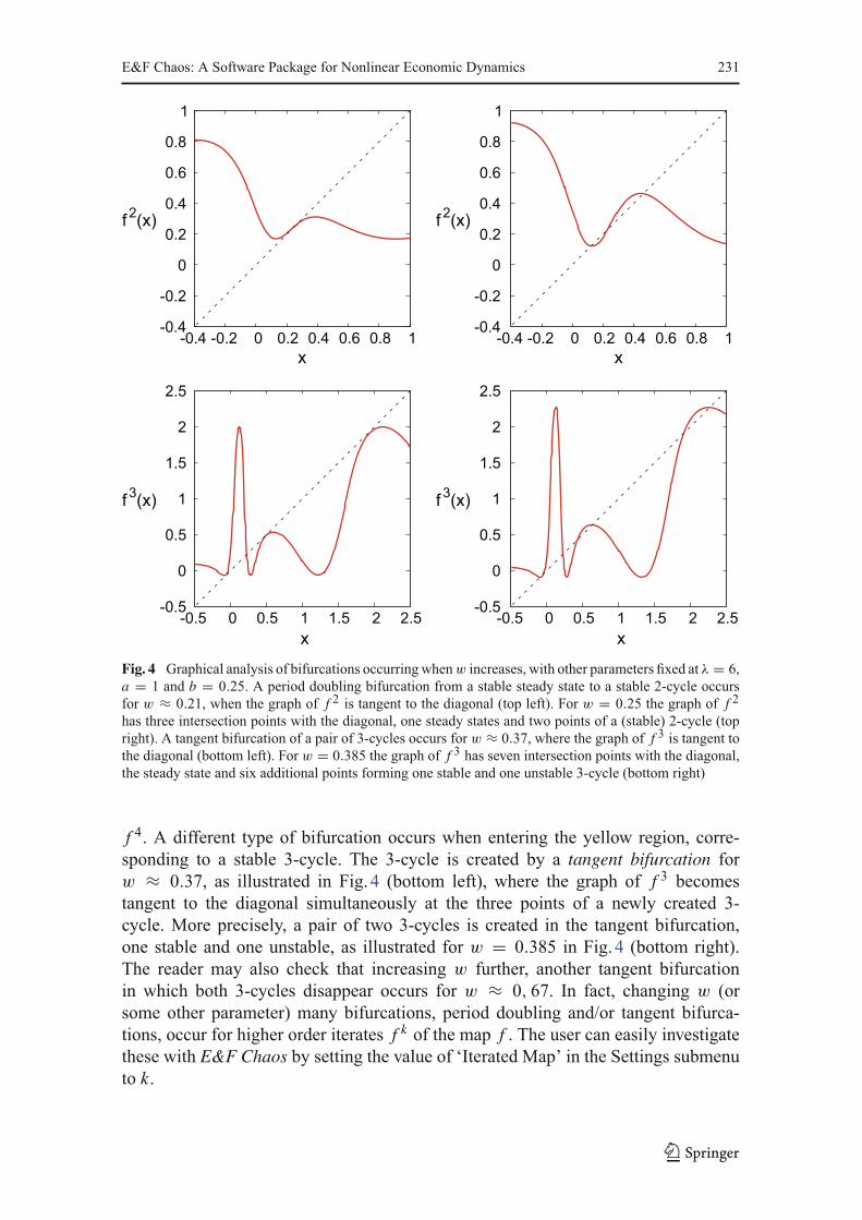
The boundaries between different colors in the parameter basins in Fig. 3 repre-sent bifurcation curves in the 2-D (λ,w)-parameter space. For 1-D systems, bifur-cations of cycles can be easily investigated by the Graphical Analysis menu. Forexample, Fig. 3 suggest that fixing λ = 6 and increasing w leads to a period dou-bling bifurcation when the dynamics changes from a stable steady state (the lightblue region) to a stable 2-cycle (the dark blue region). The graphical analysis inFig. 4 confirms this conjecture. At the bifurcation value w ≈ 0.21 (top left), thegraph of the second iterate f 2 is tangent to the diagonal at the steady state, and thesteady state is their only intersection point. Beyond the bifurcation value, as illus-trated for w = 0.25 (top right), the graph of f 2 has three intersection points withthe diagonal, namely the steady state and two additional points forming a (stable)2-cycle. The parameter basins plot in Fig. 3 suggests that more bifurcations occurwhen w is further increased. The reader may check e.g. that a second period dou-bling bifurcation occurs for w ≈ 0.28, by looking at the graphs of the fourth iterate

123


-0.4

-0.2

0

0.2

0.4

0.6

0.8

1

-0.4 -0.2 0 0.2 0.4 0.6 0.8 1

f 2(x)

x

-0.4

-0.2

0

0.2

0.4

0.6

0.8

1

-0.4 -0.2 0 0.2 0.4 0.6 0.8 1

f 2(x)

x

-0.5

0

0.5

1

1.5

2

2.5

-0.5 0 0.5 1 1.5 2 2.5

f 3(x)

x

-0.5

0

0.5

1

1.5

2

2.5

-0.5 0 0.5 1 1.5 2 2.5

f 3(x)

x

Fig. 4 Graphical analysis of bifurcations occurringwhenw increases, with other parameters fixed at λ = 6,a = 1 and b = 0.25. A period doubling bifurcation from a stable steady state to a stable 2-cycle occursfor w ≈ 0.21, when the graph of f 2 is tangent to the diagonal (top left). For w = 0.25 the graph of f 2

has three intersection points with the diagonal, one steady states and two points of a (stable) 2-cycle (topright). A tangent bifurcation of a pair of 3-cycles occurs for w ≈ 0.37, where the graph of f 3 is tangent tothe diagonal (bottom left). For w = 0.385 the graph of f 3 has seven intersection points with the diagonal,the steady state and six additional points forming one stable and one unstable 3-cycle (bottom right)

f 4. A different type of bifurcation occurs when entering the yellow region, corre-sponding to a stable 3-cycle. The 3-cycle is created by a tangent bifurcation forw ≈ 0.37, as illustrated in Fig. 4 (bottom left), where the graph of f 3 becomestangent to the diagonal simultaneously at the three points of a newly created 3-cycle. More precisely, a pair of two 3-cycles is created in the tangent bifurcation,one stable and one unstable, as illustrated for w = 0.385 in Fig. 4 (bottom right).The reader may also check that increasing w further, another tangent bifurcationin which both 3-cycles disappear occurs for w ≈ 0, 67. In fact, changing w (orsome other parameter) many bifurcations, period doubling and/or tangent bifurca-tions, occur for higher order iterates f k of the map f . The user can easily investigatethese with E&F Chaos by setting the value of ‘Iterated Map’ in the Settings submenuto k.

123

232 C. Diks et al.

4 A Higher Dimensional Example

In this section we consider a higher dimensional example of a nonlinear system,to illustrate more features of the E&F Chaos software. The model is an extensionof the agent-based cobweb model with heterogeneous expectations (rational versusnaive expectations) introduced by Brock and Hommes (1997), modified to allow forasynchronous updating of strategies. This extension allows us to illustrate how easyit is to include a new or extended model in E&F Chaos. As in the previous section,demand is linear and given by

D(pt ) = a − bpt . (6)

The supply is also assumed to be linear, derived from expected profit maximizationfrom a quadratic cost function c(q) = q2/(2s), and therefore given by

S(peht ) = speht , (7)

where peht is the expectedmarket price by agents of type h. Agents can choose betweentwo different types of expectation rules, a costly sophisticated rule and a cheap freerule. The type 1 rule is rational expectations, which can be obtained at informationgathering costs C > 0, while the type 2 rule is naive expectations, which is availableat no cost. The forecasting rules thus are

pe1t = pt , pe2t = pt−1. (8)

With rational and naive producers, the market clearing condition is given by

a − bpt = n1t spt + n2t spt−1, (9)

where n1t and n2t represent the fractions of type 1 and type 2 agents. The uniquemarket clearing price pt is then given by

pt = a − n2t spt−1b + sn1t

. (10)

The fractions are determined by the past performance of the two forecasting strate-gies. The payoff πht of strategy h at time t is given by the realized profit of thatstrategy at time t minus the costs incurred. Using producers’ quadratic cost functionc(q) = q2/(2s) and taking the constant information gathering costsC > 0 for rationalexpectations into account, one finds

π1t = b

2p2t − C, π2t = b

2pt−1(2pt − pt−1). (11)

123


The fitness measure Uht of strategy h is a geometrically downweighted average ofpast profits, i.e.

Uht = wUh,t−1 + (1− w)πht , (12)

where w ∈ [0, 1) is a memory parameter. The extreme case w = 0 represents agentsbasing their evaluation only on the profits observed in the previous period. Brock andHommes (1997) considered thismodelwith synchronous updating of strategies, that is,in each period all agents update their strategies.Herewe consider themore general caseof asynchronous updating. Per time unit only a fraction 1 − δ of agents, distributedrandomly among agents of both types and independently across time, is assumedto reconsider their strategy on the basis of the most recent information available.The remaining fraction δ continues to use their previous strategy. The correspondingdynamics of the fractions is given by a modified version of the discrete choice, logitprobabilities:

nht = (1− δ)eβUh,t−1/Zt−1 + δnh,t−1, (13)

where Zt−1 = ∑h e

βUh,t−1 is a normalization factor so that the fractions add up to 1.For δ = 0, we are back in the case of synchronous updating. In evolutionary gametheory there has been a discussion whether asynchronous updating may lead to morestability (cf. Nowak and May 1992; Huberman and Glance 1993; Nowak et al. 1992).Financial market models with asynchronous updating have been considered by Diksand van der Weide (2005) and Hommes et al. (2005).The dynamics of the cobweb model with rational versus naive agents and asyn-

chronous updating of strategies is thus given by Eqs. 10–13, defining a nonlinearfour-dimensional (with state variables pt−1, n1,t−1, U1,t−1 and U2,t−1) discrete timedynamical system. A typical research question for such a generalization of an existingmodel is how the extra parameters affect the dynamics. Our aim is to illustrate how theE&F Chaos program can help to obtain a quick overview of the (long-run) behaviorof the dynamics in different regions of the parameter space.

4.1 Building a New Model in E&F Chaos

Including a new model or modifying an existing model in the E&F Chaos software iseasy. All the user has to do is to specify the model in LUA code (or modify an exist-ing model) in a plain text file, either with the built-in editor or with her own favoriteeditor.6 To view an example, the user can use the File/Load Model submenu, openthe subdirectory ‘My Models’ and select the file ‘BH-cobweb-async’, the cobwebmodel with asynchronous updating as presented in the previous subsection. Using theFile/Edit Model submenu, a window containing the model equations appears:

6 For more information about the LUA language, see the LUA website www.lua.org.

123

234 C. Diks et al.

p=2, n1=0.5, n2=0.5, u1=0, u2=0beta=5, a=4, b=0.5, s=1.35, C=1, w=0,delta=0pchanged-- BH-cobweb-async

-- lagged variablesplag = pn1lag = n1u1lag = u1u2lag = u2

-- pricep = (a-n2*s*plag)/(b+n1*s)

-- fitnessu1 = w*u1lag + (1-w)*((b/2)*p*p-C)u2 = w*u2lag + (1-w)*(b/2)*plag*(2*p-plag)

-- fractionsq1 = math.exp(beta*u1)q2 = math.exp(beta*u2)z = q1+q2n1 = delta*n1lag + (1-delta)*q1/zn2 = 1-n1

-- price changepchange=p-plag

Strictly speaking the first four lines are not LUA code. They comprise a four lineheader to inform the E&F Chaos program about the various model parameters, statevariable and the type of model. The first line provides the state variables (p, n1, n2, u1and u2) and their default initial states. The second line specifies the model parameters(the intensity of choice β, the constant a and slope b of the demand curve, the slopes of the supply curve, the information gathering costs C , the memory w in the fit-ness measure and the parameter δ measuring asynchronous updating) as well as theirdefault values. Any additional variables (pchange, the price change) of which outputis desired are provided on the third line, while the fourth and final header line containsa letter to specify whether we are dealing with a continuous time (‘c’) or discrete time(‘d’) system. As an alternative to providing either ‘c’ or ‘d’ on the fourth line of theheader, at the bottom of the Edit Model window, the user can specify the ‘Type’ (i.e.either ‘c’ for a continuous time model or ‘d’ for discrete time). The remaining codeis used to describe the dynamical system by specifying the new values of the state

123


0 0.5

1 1.5

2 2.5

3 3.5

4

0 20 40 60 80 100

p

time

0 0.5

1 1.5

2 2.5

3 3.5

4

0 20 40 60 80 100

p, n1

time

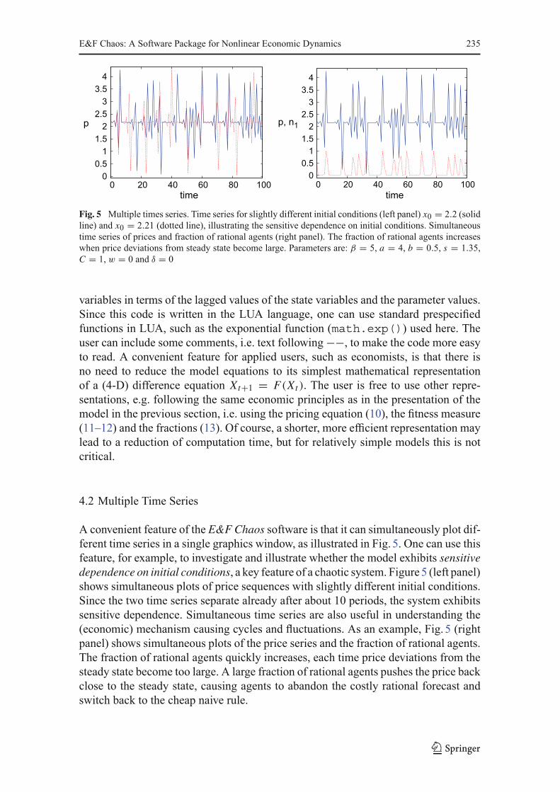
Fig. 5 Multiple times series. Time series for slightly different initial conditions (left panel) x0 = 2.2 (solidline) and x0 = 2.21 (dotted line), illustrating the sensitive dependence on initial conditions. Simultaneoustime series of prices and fraction of rational agents (right panel). The fraction of rational agents increaseswhen price deviations from steady state become large. Parameters are: β = 5, a = 4, b = 0.5, s = 1.35,C = 1, w = 0 and δ = 0

variables in terms of the lagged values of the state variables and the parameter values.Since this code is written in the LUA language, one can use standard prespecifiedfunctions in LUA, such as the exponential function (math.exp()) used here. Theuser can include some comments, i.e. text following−−, to make the code more easyto read. A convenient feature for applied users, such as economists, is that there isno need to reduce the model equations to its simplest mathematical representationof a (4-D) difference equation Xt+1 = F(Xt ). The user is free to use other repre-sentations, e.g. following the same economic principles as in the presentation of themodel in the previous section, i.e. using the pricing equation (10), the fitness measure(11–12) and the fractions (13). Of course, a shorter, more efficient representation maylead to a reduction of computation time, but for relatively simple models this is notcritical.

4.2 Multiple Time Series

A convenient feature of the E&F Chaos software is that it can simultaneously plot dif-ferent time series in a single graphics window, as illustrated in Fig. 5. One can use thisfeature, for example, to investigate and illustrate whether the model exhibits sensitivedependence on initial conditions, a key feature of a chaotic system. Figure5 (left panel)shows simultaneous plots of price sequences with slightly different initial conditions.Since the two time series separate already after about 10 periods, the system exhibitssensitive dependence. Simultaneous time series are also useful in understanding the(economic) mechanism causing cycles and fluctuations. As an example, Fig. 5 (rightpanel) shows simultaneous plots of the price series and the fraction of rational agents.The fraction of rational agents quickly increases, each time price deviations from thesteady state become too large. A large fraction of rational agents pushes the price backclose to the steady state, causing agents to abandon the costly rational forecast andswitch back to the cheap naive rule.

123

236 C. Diks et al.

0.1

0.2

0.3

0.4

0.5

0.6

3 4 5 6 7 8

n1

p

3

4

5

6

7

8

3 4 5 6 7 8

pt+1

pt

Fig. 6 Phase plot (left panel) with a strange attractor in the (p, n1) plane. The same attractor shown in adelay plot (pt , pt+1) (right panel). Parameters are: β = 15, a = 10, b = 0.5, s = 1.35, C = 1, w = 0 andδ = 0.8

4.3 Phase Plots and Delay Plots

For higher dimensional systems, Phase Plots and Delay Plots provide helpful toolsto investigate the (long run) dynamical behavior and plot attractors of the system.Intuitively, an attractor of a dynamical system is the subset of state space points towhich the dynamics are confined in the long run. The attractor thus contains infor-mation about the long run dynamical behavior of the system. Examples are a stablesteady state (single point attractor), a stable periodic orbit (finite number of points),a quasi-periodic attractor (“invariant circle”) and a strange (chaotic) attractor (fractalstructure). Examples of a phase plot and a delay plot of a strange attractor are shownin Fig. 6. By holding the mouse button and drawing a rectangle, the user can zoominto the detailed fractal structure of the attractor.

4.4 Iterating Objects: The Unstable Manifold of the Steady State

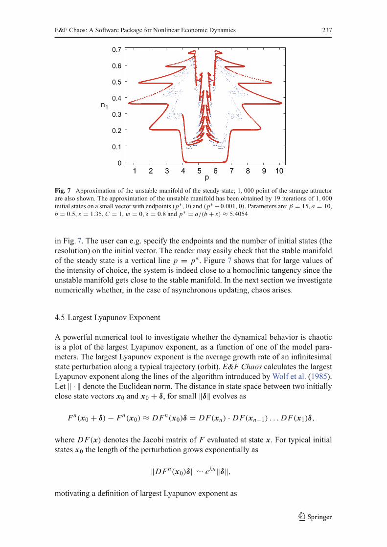
The attractors in Fig. 6 correspond to the case of asynchronous updating (δ = 0.8) andno memory in the fitness measure (w = 0). In this case, mathematically the systemcan be reduced to a 2-D system. In the case of synchronous updating of strategies(δ = 0), Brock and Hommes (1997) have shown that, for large values of the intensityof choice β the system is close to a homoclinic tangency between the stable andunstable manifolds of the steady state. The strange attractor in Fig. 6 suggests thata near homoclinic tangency may also explain the complicated dynamics in the caseof asynchronous updating of strategies. A mathematical analysis is beyond the scopeof this paper (for a mathematical treatment of homoclinic bifurcations see e.g. Palisand Takens 1993), but we can use the Iterating Objects submenu to approximate theunstable manifold of the steady state. The user can iterate circles as well as polygonsover the attractor. Iterating small circles can e.g. illustrate the sensitive dependenceand how quickly nearby points spread over a strange attractor. The option of Iteratinga polygon and setting the number of vertices to two enables the user to iterate vectors.This option can then be used to iterate a small unstable eigenvector originating at thesteady state thus approximating the unstable manifold of the steady state, as illustrated

123


0

0.1

0.2

0.3

0.4

0.5

0.6

0.7

1 2 3 4 5 6 7 8 9 10

n1

p

Fig. 7 Approximation of the unstable manifold of the steady state; 1, 000 point of the strange attractorare also shown. The approximation of the unstable manifold has been obtained by 19 iterations of 1, 000initial states on a small vector with endpoints (p∗, 0) and (p∗ +0.001, 0). Parameters are: β = 15, a = 10,b = 0.5, s = 1.35, C = 1, w = 0, δ = 0.8 and p∗ = a/(b + s) ≈ 5.4054

in Fig. 7. The user can e.g. specify the endpoints and the number of initial states (theresolution) on the initial vector. The reader may easily check that the stable manifoldof the steady state is a vertical line p = p∗. Figure 7 shows that for large values ofthe intensity of choice, the system is indeed close to a homoclinic tangency since theunstable manifold gets close to the stable manifold. In the next section we investigatenumerically whether, in the case of asynchronous updating, chaos arises.

4.5 Largest Lyapunov Exponent

A powerful numerical tool to investigate whether the dynamical behavior is chaoticis a plot of the largest Lyapunov exponent, as a function of one of the model para-meters. The largest Lyapunov exponent is the average growth rate of an infinitesimalstate perturbation along a typical trajectory (orbit). E&F Chaos calculates the largestLyapunov exponent along the lines of the algorithm introduced by Wolf et al. (1985).Let ‖ · ‖ denote the Euclidean norm. The distance in state space between two initiallyclose state vectors x0 and x0 + δ, for small ‖δ‖ evolves as

Fn(x0 + δ) − Fn(x0) ≈ DFn(x0)δ = DF(xn) · DF(xn−1) . . . DF(x1)δ,

where DF(x) denotes the Jacobi matrix of F evaluated at state x. For typical initialstates x0 the length of the perturbation grows exponentially as

‖DFn(x0)δ‖ ∼ eλn‖δ‖,

motivating a definition of largest Lyapunov exponent as

123

238 C. Diks et al.

λ = limn→∞

1nlog

‖DFn(x0)δ‖‖δ‖ .

4.5.1 Algorithm for Lyapunov exponent

Generally speaking, λ can be estimated numerically either by specifying the Jacobimatrix analytically, evaluating it at any point along a generated orbit, or by using a finitedifferencing method along the orbit. Wolf et al. (1985) opt for the first method in casethe dynamics are known, while they use the second approach in case the dynamicsis reconstructed from an observed time series. We use a finite difference approachalso in the case of known dynamics, thus avoiding an error prone specification ofthe Jacobi matrix by the user. The price payed is a slight loss of accuracy due to thefinite difference approximation and numerical noise, but for most practical purposesthe differences are sufficiently small, especially when the number of iterations is large(e.g. about 10,000).The main idea behind the finite differencing algorithm for the largest Lapunov

exponent is to follow the evolution of a small initial disturbance of the state around areference trajectory (assumed to be typical orbit generated by the dynamics). To pre-vent the distance between the disturbed and the reference trajectory from becomingtoo large, this distance is regularly (in our implementation every time step) rescaledto a small number ε while keeping the direction of the disturbance unaffected. Inpseudocode:

Set r = 0Take an initial vector x0 and a perturbed vector x + δ0 with ‖δ0‖ = ε.For t = 1, . . . , n{

iterate both states: xt = F(xt−1) and xt + δ′t−1 := F(xt−1 + δt−1)

Sum up the growth rate along the orbit: r = r + log ‖δ′t−1‖‖ε‖

Rescale the perturbation δ′t−1 to length ε through xt + δt := xt + ‖ε‖

‖δ′t−1‖δ′

t−1.}Estimate λ as te average growth rate r/n.

The perpetual rescaling of the perturbation is used to keep the distance betweenthe reference and the perturbed trajectory small. In this way the evolution of a tan-gent vector along the trajectory is approximated, allowing the difference betweenthe two trajectories to evolve towards the most unstable direction of the dynamics,which is the direction associated with the largest Lyapunov exponent. The initial dis-turbance is chosen to be a positive change of size ε of the first element of the statevariable.Figure8 shows a bifurcation diagram and a Lyapunov exponent plot with respect to

the intensity of choice parameter β, in the case of asynchronous updating of strategies(δ = 0.8). The bifurcation diagram (top panel) shows a primary period doublingbifurcation (froma stable steady state to a stable 2-cycle), a secondaryHopf bifurcationof the 2-cycle (the reader may check this by a phase plot of the attractor for e.g. β = 3,

123


1

2

3

4

5

0 5 10 15 20

p

β

-0.2

-0.15

-0.1

-0.05

0

0.05

0.1

2 4 6 8 10 12 14 16 18 20

LE

β

Fig. 8 Bifurcation diagram (top panel) and largest Lyapunov exponent (LE) plot (bottom panel) in the caseof asynchrounous updating of strategies. The bifurcation diagram shows the long run dynamical behavior,100 iterations after a transient of 100 iterations, as a function of the parameter β. The LE plot is based on5000 iterations after a transient of 300 iterations and takes 35s (Pentium 3GHz). Other parameters are:a = 6, b = 0.5, s = 1.35, C = 1, w = 0 and δ = 0.8

showing the invariant circles created in theHopf bifurcation), followed by a bifurcationroute to more complicated dynamical behavior. The Lyapunov exponent plot (bottompanel) becomes positive for large values of β, providing numerical evidence that thedynamics becomes chaotic for large values of the intensity of choice. These simulationsthus show that the rational route to randomness, that is, the bifucation route to chaos,found by Brock and Hommes (1997) in the cobweb model with synchronous updatingof strategies also arises in the case of asynchronous updating of strategies.Using the Largest Lyapunov Exponent submenu, the user can specify the parameter,

the range of the parameter, the size of the perturbation vector (default at 0.001), thenumber of iterations and the transient time for computation of theLyapunov exponents.The output is given as a graph of the estimated largest Lyapunov exponent as a functionof this parameter range. If required the resolution in the parameter space canbe adjustedby the user.

123

240 C. Diks et al.

0

0.2

0.4

0.6

0.8

1

-1.5 -1 -0.5 0 0.5 1 1.5

n1

x

0

0.2

0.4

0.6

0.8

1

-1.5 -1 -0.5 0 0.5 1 1.5

n1

x

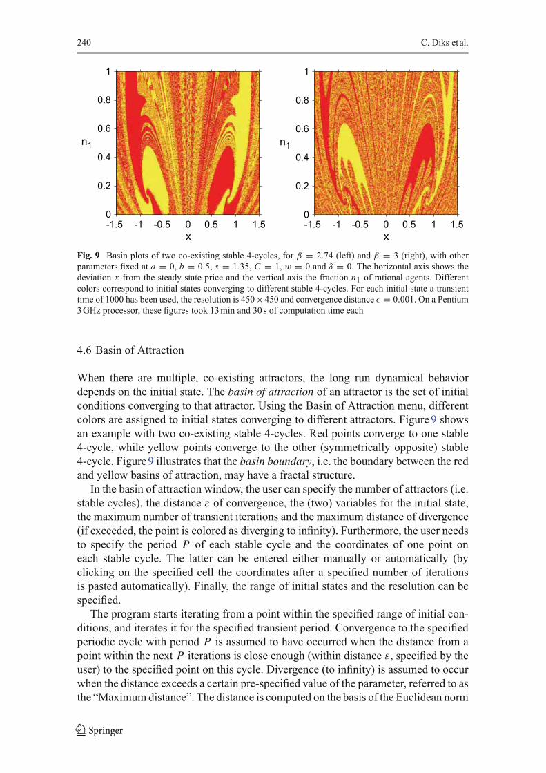
Fig. 9 Basin plots of two co-existing stable 4-cycles, for β = 2.74 (left) and β = 3 (right), with otherparameters fixed at a = 0, b = 0.5, s = 1.35, C = 1, w = 0 and δ = 0. The horizontal axis shows thedeviation x from the steady state price and the vertical axis the fraction n1 of rational agents. Differentcolors correspond to initial states converging to different stable 4-cycles. For each initial state a transienttime of 1000 has been used, the resolution is 450×450 and convergence distance ε = 0.001. On a Pentium3GHz processor, these figures took 13min and 30s of computation time each

4.6 Basin of Attraction

When there are multiple, co-existing attractors, the long run dynamical behaviordepends on the initial state. The basin of attraction of an attractor is the set of initialconditions converging to that attractor. Using the Basin of Attraction menu, differentcolors are assigned to initial states converging to different attractors. Figure9 showsan example with two co-existing stable 4-cycles. Red points converge to one stable4-cycle, while yellow points converge to the other (symmetrically opposite) stable4-cycle. Figure9 illustrates that the basin boundary, i.e. the boundary between the redand yellow basins of attraction, may have a fractal structure.In the basin of attraction window, the user can specify the number of attractors (i.e.

stable cycles), the distance ε of convergence, the (two) variables for the initial state,the maximum number of transient iterations and the maximum distance of divergence(if exceeded, the point is colored as diverging to infinity). Furthermore, the user needsto specify the period P of each stable cycle and the coordinates of one point oneach stable cycle. The latter can be entered either manually or automatically (byclicking on the specified cell the coordinates after a specified number of iterationsis pasted automatically). Finally, the range of initial states and the resolution can bespecified.The program starts iterating from a point within the specified range of initial con-

ditions, and iterates it for the specified transient period. Convergence to the specifiedperiodic cycle with period P is assumed to have occurred when the distance from apoint within the next P iterations is close enough (within distance ε, specified by theuser) to the specified point on this cycle. Divergence (to infinity) is assumed to occurwhen the distance exceeds a certain pre-specified value of the parameter, referred to asthe “Maximumdistance”. The distance is computed on the basis of the Euclidean norm

123


using either the two-dimensional space for which the basins are plotted or all dimen-sions of the model (if the “All dim.” box is checked). ‘Non Convergence’ is reported,when the point has not reached one of the stable cycles within the specified distanceafter the specified transient. The parameter “Resolution” determines howmany pointsfrom the range of initial values are used in the algorithm. The default value is set tothe maximum screen resolution, but initial explorations with lower resolution (e.g.100) is recommended, because high resolution basin plots are computationally inten-sive.

5 Simulations with Noise

There are a few remaining features ofE&FChaoswewould like tomention.TheBasicsmenu contains two submenus, Spreadsheet and Statistics. The Spreadsheet option isvery helpful in saving numerical values of all variables.As all other graphicalwindows,the Spreadsheet window has an Edit/Parameters submenuwhere parameters and initialstates can bemodified. The user can also specify the first point and the number of pointsto be computed. Using the File/Save as submenu, the data can be saved as a text file.The Basics/Statistics menu allows the user to compute some basic statistics of a timeseries, such as the mean, median, maximum, minimum, standard deviation, variance,and the skewness and kurtosis coefficients.An important question, particularly relevant for economics, is how noise affects the

dynamics of a nonlinear system. The user can include simulated noise in the modeldirectly in the LUA code using the LUA random number generator math.random,which is an interface to the well-documented ANSI C random number generatorrand(). However, for the convenience of the user, E&F Chaos also has a built-in noise option using the Delphi Pascal noise generator, intended for obtaining aquick impression of the effect of additive noise with various distributions on the statevariables. Upon clicking the Extra/Noise submenu, the Noise window appears, wherethe user can select the distribution of the noise (uniform, normal or double exponential),the standard deviation of the noise and the variable to which the noise should be added.The default option is then that in each time step a noise term is added to the selectedvariable after each iteration. The user has two additional options, to add a noise termonly each k-th period or to select a probability p with which the noise is added ineach period. In this way, the user can easily investigate how noise affects the nonlineardynamics.As an example, Fig. 10 shows the same bifurcation diagram as in Fig. 2, subject to

dynamic noise. In each time step, a normally distributed random variable εt , with zeromean and standard deviation 0.1 has been added to the RHS of the dynamics of theexpected price in Eq. 5. The figure shows that the detailed structure of the bifurcationdiagramdisappears.However, in the presence of noise price fluctuations exhibit similarfeatures as in the noise free case. For small values of the parameter w, 0 ≤ w ≤ 0.3,price fluctuations are close to the steady state, for large values of w, w > 0.8, pricesexhibit up and down oscillations (a noisy 2-cycle), while for intermediate values ofw, 0.3 < w < 0.7 price fluctuations are complicated. An observant reader may stilldetect a noisy 4-cycle in the bifurcation diagram in Fig. 10, for 0.7< w < 0.75.

123

242 C. Diks et al.

Fig. 10 Bifurcation diagram asin Fig. 2, buffeted with noise εt ,normally distributed with SD0.1. The diagram shows the longrun behavior (100 iterations)after a transient of 100 iterations

0

2

4

6

8

0.2 0.3 0.4 0.5 0.6 0.7 0.8 0.9

x

w

6 Summary

In this paper we have described the E&F Chaos software package for simulating andanalyzing nonlinear economic dynamical systems. The current version is an upgradedversion of an earlier program, the main added features being the ability for the user toeasily specify newmodels in the LUA language without the need of a compiler, as wellas the ability to generate publication quality graphical output. The paper illustrates howthe different features of the program can be used when the E&F Chaos is employedfor carrying out its primary task, which is to aid students and researchers in the initialstages with a quick numerical analysis of the dynamical features of newly specifiednonlinear models. To this end we have considered two case studies, comprising ofboth a one-dimensional and a higher-dimensional economic dynamic model, and havedescribed in detail how theE&FChaos program could be utilized for quickly obtainingan overview of the dynamical properties of these models, and how E&F Chaos canhelp formulate more advanced research questions for further analysis. In addition,we briefly discussed the program’s built-in feature to investigate how noise affectsthe nonlinear dynamics. We hope that this software package will contribute to moreapplications of nonlinear dynamics in economics and finance, and make it easier fornon-specialists to discover the intriguing features of nonlinear dynamics.

Acknowledgments This paper was presented at the Fourth Workshop Modelli Dinamici in Economia eFinanza, September 21–23, 2006, Urbino, Italy. We thank all participants for helpful comments.

Open Access This article is distributed under the terms of the Creative Commons Attribution Noncom-mercial License which permits any noncommercial use, distribution, and reproduction in any medium,provided the original author(s) and source are credited.

References

Arrowsmith, D. K., & Place, C. M. (1995). An introduction to dynamical systems. Cambridge: CambridgeUniversity Press.

123


Boldrin, M., & Woodford, M. (1990). Equilibrium models displaying endogenous fluctuations and chaos:A survey. Journal of Monetary Economics, 25, 189–222.

Brock, W. A., & Hommes, C. H. (1997). A rational route to randomness. Econometrica, 65, 1059–1095.Brock, W. A., Hsieh, D. A., & LeBaron, B. (1991). Nonlinear dynamics, chaos and instability: Statistical

theory and economic evidence. Cambridge: MIT Press.Chiarella, C. (1988). The cobweb model: Its instability and the onset of chaos. Economic Modeling, 5,377–384.

Day, R. H. (1994). Complex economic dynamics. Volume I: An introduction to dynamical systems andmarket mechanisms. Cambridge: MIT Press.

Devaney, R. L. (1989). An introduction to chaotic dynamical systems (2nd ed.). Redwood City: AddisonWesley Publication.

Diks, C. G. H., & van derWeide, R. (2005). Herding, a-synchronous updating and heterogeneity in memoryin a CBS. Journal of Economic Dynamics and Control, 29, 741–763.

Doedel, E. J., Paffenroth, R. C., Champneys, A. R., Fairgrieve, T. F., Kuznetsov, Y. A., Oldeman, B. E.,Sandstede, B., & Wang, X. J. (2001). AUTO2000: Continuation and bifurcation software for ordinarydifferential equations. Applied and Computational Mathematics. California Institute of Technology.http://indy.cs.concordia.ca/auto/.

Ezekiel, M. (1938). The cobweb theorem. Quarterly Journal of Economics, 52, 255–280.Grandmont, J.-M. (1985). On endogenous competitive business cycles. Econometrica, 53, 995–1046.Grandmont, J.-M. (1988). Nonlinear difference equations, bifurcations and chaos: An introduction.CEPREMAP Working Paper No 8811, June 1988.

Guckenheimer, J., & Holmes, P. (1983). Nonlinear oscillations, dynamical systems, and bifurcations ofvector fields. New York: Springer Verlag.

Hommes, C. H. (1991). Chaotic dynamics in economic models. Some simple case-studies. GroningenTheses in Economics, Management & Organization, Wolters-Noordhoff, Groningen.

Hommes, C. H. (1994). Dynamics of the cobweb model with adaptive expectations and nonlinear supplyand demand. Journal of Economic Behavior & Organization, 24, 315–335.

Hommes, C. H. (2006). Heterogeneous agent models in economics and finance, In L. Tesfatsion &K. L. Judd (eds.), Handbook of computational economics, volume 2: Agent-based computationaleconomics (pp. 1109–1186). Amsterdam: North-Holland, Chap. 23.

Hommes, C. H., Huang, H., & Wang, D. (2005). A robust rational route to randomness in a simple assetpricing model. Journal of Economic Dynamics and Control, 29, 1043–1072.

Huberman, B. A., & Glance, N. S. (1993). Evolutionary games and computer simulations. Proceedings ofthe National Academy of Sciences of the United States of America, 90, 7716–7718.

Kuznetsov, Y. (1995). Elements of applied bifurcation theory. New York: Springer Verlag.LeBaron, B. (2006), Agent-based computational finance. In L. Tesfatsion & K. L. Judd (eds.), Hand-

book of computational economics, volume 2: Agent-based computational economics (pp. 1187–1233).Amsterdam: North-Holland, Chap. 24.

Li, T. Y., & Yorke, J. A. (1975). Period three implies chaos. American Mathematical Monthly, 82, 985–992.Medio, A. (1992). Chaotic dynamics. Theory and applications to economics. Cambridge: CambridgeUniversity Press.

Medio, A., & Lines, M. (2001) Nonlinear dynamics: A primer. Cambridge: Cambridge University Press.Mira, C., Gardini, L., Barugola, A., & Cathala, J.-C. (1996). Chaotic dynamics in two-dimensional nonin-

vertible maps. Singapore: World Scientific.Muth, J. F. (1961). Rational expectations and the theory of price movements. Econometrica, 29, 315–335.Nerlove, M. (1958). Adaptive expectations and cobweb phenomena. Quarterly Journal of Economics, 72,227–240.

Nowak, M., & May, R. M. (1992). Evolutionary games and spatial chaos. Nature, 359, 826–929.Nowak,M., Bonhoeffer, S., &May, R.M. (1992). Spatial and the maintainance of cooperation.Proceedings

of the National Academy of Sciences of the United States of America, 91, 4877–4881.Nusse, H. E., & Yorke, J. A. (1998). Dynamics: Numerical explorations (2nd ed.). Applied MathematicalSciences (Vol. 101). Springer-Verlag.

Palis, J., & Takens, F. (1993). Hyperbolicity and sensitive chaotic dynamics at homoclinic bifurcations.Cambridge: Cambridge University Press.

Racine, J. (2006). gnuplot 4.0: A portable interactive plotting utility. Journal of Applied Econometrics, 21,133–141.

123

244 C. Diks et al.

Rosser, J. B. (2000). From catastrophe to chaos: A general theory of economic discontinuities. Boston:Kluwer.

Wolf, A., Swift, J. B., Swinney, L., & Vastano, J. A. (1985). Determining Lyapunov exponents from a timeseries. Physica D, 16, 285–317.

123

e&f chaos: a user friendly software package for nonlinear...

Documents