efficient estimation of the parameterpathinunstable time
TRANSCRIPT

Review of Economic Studies (2010) 77, 1508–1539 0034-6527/10/00411011$02.00© 2010 The Review of Economic Studies Limited doi: 10.1111/j.1467-937X.2010.00603.x
Efficient Estimation of theParameter Path in Unstable
Time Series ModelsULRICH K. MULLER and
PHILIPPE-EMMANUEL PETALASPrinceton University
First version received February 2008; final version accepted November 2009 (Eds.)
The paper investigates inference in non-linear and non-Gaussian models with moderately time-varying parameters. We show that for many decision problems, the sample information about theparameter path can be summarized by an artificial linear and Gaussian model, at least asymptotically.The approximation allows for computationally convenient path estimators and parameter stability tests.Also, in contrast to standard Bayesian techniques, the artificial model can be robustified so that inmisspecified models, decisions about the path of the (pseudo-true) parameter remain as good as in acorresponding correctly specified model.
1. INTRODUCTION
One of the central concerns in time series modelling is the stability of parameters throughtime. A large body of econometric work has developed around testing the hypothesis thatparameters are time invariant; see Stock (1994) and Dufour and Ghysels (1996) for surveysand references. Empirically, there is substantial evidence of instabilities in the parametersof finance and macroeconomic models as documented in Stock and Watson (1996), Ghysels(1998), Primiceri (2005) and Cogley and Sargent (2005), just to name a few.
Once instabilities are suspected, a natural next step is to document their form. Knowledge ofthe parameter path is useful for a number of purposes. First, the estimated path is an interestingdescriptive tool, as it helps to understand potential sources of the instability. Second, the endpoint of the parameter path is useful for forecasting purposes. Third, economic theory mightimply certain features of parameter paths (think, for instance, of convergence models withtime-varying mean growth of GDP), for which one might want to test in econometric models.Finally, the time-varying value of the parameter can sometimes be given a useful structuralinterpretation, such as a time-dependent marginal effect in a regression model.
There are several approaches to estimating the parameter path. One strand develops fre-quentist inference for the break date in models where the parameters are known a priori to besubject to a small number of sudden shifts, such as Bai (1997), Bai and Perron (1998), andElliott and Muller (2007). A Bayesian literature (e.g. Hamilton, 1989; Chib, 1998; Sims andZha, 2006) posits a finite number of regimes for the parameter values and obtains posteriorprobabilities for each regime through time. Priestley and Chao (1972), Robinson (1989, 1991),Wu and Zhao (2007), and Cai (2007), among others, develop non-parametric kernel estimators
1508

MULLER & PETALAS PARAMETER PATH IN UNSTABLE TIME SERIES MODELS 1509
of the time-varying parameter. Finally, a large frequentist and Bayesian literature estimatesmodels under the assumption of a smooth stochastic evolution of the parameter. When theparameters enter the model linearly and disturbances are assumed Gaussian, then these modelscan be estimated by variants of Kalman filtering and smoothing—see Harvey (1989) for areview. This is not possible for models with time-varying parameters that affect, say, variancesand covariances, and considerably more involved numerical techniques have been developed todeal with such models: see, for instance, Harvey, Ruiz, and Shephard (1994), Jacquier, Polson,and Rossi (1994), Durbin and Koopman (1997), Shephard and Pitt (1997), Kim, Shephard,and Chib (1998), and Primiceri (2005) for the estimation of models with time-varying secondmoments. In general, the estimation of time-varying parameter models outside the Gaussianstate space framework requires fairly complicated and model-specific numerical techniques.
This paper is closely related to this last strand. We consider a general parametric model withlocal time variation, in the sense that good tests would detect the instability with probabilitysmaller than 1 even in the limit. We analyse estimators and tests that minimize weighted averagerisk (WAR) and maximize weighted average power over the set of possible parameter paths,where the weighting function is proportional to the distribution function of a Gaussian process,and focuses on such local parameter variability. The main contribution is an asymptoticallyaccurate approximation to the sample information about the parameter path. This approximationturns the problem of inference about the parameter path in the general likelihood model intothe problem of inference about the parameter path in a linear Gaussian pseudo model, with thesequence of scores (evaluated at the usual maximum likelihood estimator) as the observations.Asymptotically efficient parameter path estimators and test statistics thus become straightfor-ward to compute, and the estimation and testing problem are unified in one coherent asymptoticframework. In the special case of an underlying parametric model that is stationary for stableparameters, and a weighting that corresponds to the distribution of a Gaussian random walk,the approximate pseudo model can be chosen as a local level model in the sense of Harvey(1989), and optimal path estimators are obtained by an exponential smoothing of the sequenceof score vectors. From a Bayesian perspective with the weighting function interpreted as theprior, our results provide an asymptotically accurate multivariate Gaussian approximation tothe posterior distribution of the parameter path.
When the likelihood is misspecified, exact Bayesian inference no longer minimizes WARby construction, even for losses about the pseudo-true parameter value in the sense of White(1982). We extend the ideas in Muller (2009) to construct a robustified pseudo model around the“sandwich” covariance matrix which yields as good asymptotic inference about the parameterpath as one would obtain from a correctly specified model with Fisher information equal tothe inverse of the sandwich covariance matrix. This robustness property further strengthens theappeal of the suggested approximation over the computationally intensive Bayesian solution,which cannot be easily robustified in the same fashion. Even if the original model is Gaussianand linear, so that the pseudo model approximation can be chosen to be exact in the correctlyspecified model, inference becomes more reliable in large samples by replacing the originallikelihood by the robustified pseudo model.
The asymptotics considered in this paper are such that the magnitude of the instabilitydecreases as the sample size increases. Even asymptotically, there is only limited informationabout the form of the instability (in contrast to the set-up underlying the non-parametric kernelestimators). We stress that parameter variations that are “small” in the statistical sense ofbeing non-trivial to detect need not be small in an economic sense. For instance, in a stylizedmodel, a sudden shift of 1.2 percentage points in yearly GDP mean growth in the middleof a sample of 180 quarterly observations is detected less than half the time by 5% levelefficient stability tests (Elliott and Muller, 2007), yet such a shift is arguably of major economic
© 2010 The Review of Economic Studies Limited

1510 REVIEW OF ECONOMIC STUDIES
(and policy) relevance. Many instabilities that economists care about, such as those arisingfrom Lucas-critique arguments (for instance Linde, 2001), the stability of monetary policy(for instance Bernanke and Mihov, 1998), or reduced-form bivariate econometric relationshipsbetween macroeconomic variables in general (Stock and Watson, 1996) have been difficult (or atleast non-trivial) to determine empirically and are hence “small” in the statistical sense. In theseinstances, accurate approximations might well be generated by a modelling strategy in which,correspondingly, there is only limited statistical information about the instability asymptotically.
Our results are driven by a quadratic approximation to the log-likelihood of the generalmodel. Such approximations of the likelihood for models with a finite dimensional parameterhave a long history in statistics and econometrics and allow the substitution of a complexdecision problem by a simpler one—see, for instance, LeCam (1986). Recent applications intime-series econometrics include Andrews and Ploberger (1994), Phillips and Ploberger (1996),and Ploberger (2004). The sample information about the parameter path is more difficult toapproximate, as the path is not finite dimensional. Some numerical methods for time seriesmodels with latent variables, such as those developed by Durbin and Koopman (1997) andShephard and Pitt (1997)—see Durbin and Koopman (2001) for an overview—employ sim-ilar quadratic expansions of the log-likelihood at some stage. Brown and Low (1996) andNussbaum (1996) prove the asymptotic equivalence of some specific infinite dimensional deci-sion problems with the continuous time problem of observing Gaussian white noise with someunknown drift. These papers (essentially) establish the asymptotic equivalence of the frequentistrisk for any bounded loss function. Compared to this literature, our results are more specific,as we only show equivalence with respect to WAR, where the weighting functions correspondto the distribution of a (finite mixture of) Gaussian processes. At the same time, our results aresubstantially more general, as they apply to a wide class of parametric time series models.
The remainder of the paper is organized as follows. The next section heuristically derivesthe approximating pseudo model, provides a simple algorithm for the path estimator andparameter stability test statistics for a random walk weighting function, and numerically illus-trates the ideas with the problem of estimating time-varying variances. Section 3 containsthe formal discussion of our results, and Section 4 concludes. All proofs are collected in theAppendix.
2. MOTIVATION AND DEFINITION OF EFFICIENT PARAMETER PATHESTIMATORS AND STABILITY TESTS
2.1. Heuristic derivation of approximating pseudo model
Consider a stationary and stable time series model with known log-likelihood function ofthe form
∑Tt=1 lt (θ ), with parameter θ ∈ � ⊂ Rk . The corresponding unstable model has the
same likelihood with time-varying parameter {θt }Tt=1 = {θ + δt }T
t=1. Suppose the researcher isinterested in obtaining path estimators of low expected loss for some given loss function, thatis, low risk. Risk depends on the true parameter path {θ + δt }T
t=1, and no estimator achievesuniformly low risk over all such paths. A reasonable frequentist criterion for the quality ofa path estimator thus is WAR, where the weighting is over alternative true parameter paths.In particular, in this paper we derive asymptotically WAR minimizing path estimators for adiffuse weighting of baseline value θ , and a weighting function for the deviations {δt }T
t=1 thatcorrespond to the distribution of a Gaussian process of magnitude T −1/2.
The sample information about the path {θ + δt }Tt=1 is fully contained in the function∑
lt (θ + δt ), where “∑
” denotes a sum over t = 1, . . . , T . Let θ be the maximum like-lihood estimator of θ ignoring parameter instability, i.e. θ maximizes
∑lt (θ ). Denote by
© 2010 The Review of Economic Studies Limited
MULLER & PETALAS PARAMETER PATH IN UNSTABLE TIME SERIES MODELS 1511
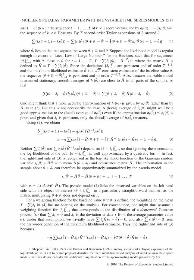
st (θ ) = ∂lt (θ )/∂θ the sequence t = 1, . . . , T of k × 1 score vectors, and by ht (θ ) = −∂st (θ )/∂θ ′the sequence of k × k Hessians. By T second-order Taylor expansions of lt around θ∑
(lt (θ + δt ) − lt (θ )) = ∑[st (θ )′(θ + δt − θ) − 1
2 (θ + δt − θ)′ht (θt )(θ + δt − θ)] (1)
where θt lies on the line segment between θ + δt and θ . Suppose the likelihood model is regularenough to ensure a “Local Law of Large Numbers” for the Hessians, such that for sequences{θt }T
t=1 with θt close to θ for t = 1, . . . , T , T −1 ∑ ht (θt ) − Hp−→ 0, where the matrix H is
defined as H = T −1 ∑ ht (θ ). Since the deviations {δt }Tt=1 are persistent and of order T −1/2,
and the maximum likelihood estimator θ is a√
T -consistent estimator of the baseline value θ ,the sequence {θ + δt − θ}T
t=1 is persistent and of order T −1/2. Also, because the stable modelis assumed stationary, smooth averages of ht (θt ) are close to H in all parts of the sample, sothat ∑
(θ + δt − θ)′ht (θt )(θ + δt − θ) � ∑(θ + δt − θ)′H (θ + δt − θ ). (2)
One might think that a more accurate approximation of ht (θt ) is given by ht (θ ) rather than byH as in (2). But this is not necessarily the case. A (local) average of ht (θ) might well be agood approximation to the (local) average of ht (θt ) even if the approximation ht (θt ) � ht (θ) ispoor, and given that δt is persistent, only the (local) average of ht (θt ) matters.
Using (2), we obtain∑(lt (θ + δt ) − lt (θ ) − 1
2 st (θ)′H −1st (θ))
� − 12
∑(st (θ) − H (θ + δt − θ ))′H −1(st (θ) − H (θ + δt − θ)). (3)
Neither∑
lt (θ) nor∑
st (θ)′H −1st (θ ) depend on {θ + δt }Tt=1, so that ignoring these constants,
the log-likelihood of the path {θ + δt }Tt=1 is well approximated by a quadratic form.1 In fact,
the right-hand side of (3) is recognized as the log-likelihood function of the Gaussian randomvariable st (θ) + H θ with mean H (θ + δt ) and covariance matrix H . The information in thesample about θ + δt can therefore be approximately summarized by the pseudo model
st (θ) + H θ = H (θ + δt ) + νt , t = 1, . . . , T (4)
with νt ∼ i .i .d .N(0, H ). The pseudo model (4) links the observed variables on the left-handside with the object of interest {θ + δt }T
t=1 in a particularly straightforward manner, as thematrix multiplying θ + δt does not depend on t .
For a weighting function for the baseline value θ that is diffuse, the weighting on the meanT −1 ∑ δt in (4) has no bearing on the analysis. For convenience, one might thus assume aweighting function for {δt }T
t=1 that corresponds to the distribution of a demeaned Gaussianprocess (so that
∑δt = 0 and δt is the deviation at date t from the average parameter value
θ ). Under that assumption, we trivially have∑
δ′t H (θ − θ) = 0, and also
∑st (θ ) = 0 from
the first-order condition of the maximum likelihood estimator. Thus, the right-hand side of (3)becomes
− 12
∑(st (θ ) − H δt )′H −1(st (θ ) − H δt ) − 1
2 T (θ − θ)′H (θ − θ )
1. Shephard and Pitt (1997) and Durbin and Koopman (1997) employ second-order Taylor expansion of thelog-likelihood as in (1) to derive proposal densities for their simulation based analysis of non-Gaussian state spacemodels, but they do not consider the additional simplification of the approximating model provided by (2).
© 2010 The Review of Economic Studies Limited

1512 REVIEW OF ECONOMIC STUDIES
and the sample information about θ and {δt }Tt=1 is approximately independent and described
by the pseudo model
θ = θ + T −1/2H −1ν0 (5)
st (θ ) = H δt + νt , t = 1, . . . , T (6)
with νt ∼ i .i .d .N(0, H ). The approximation in (5) is the standard Bernstein–von Mises resultthat in large samples, the likelihood about a parameter converges to that of a Gaussian randomvariable with mean θ and covariance matrix T −1H −1. The focus and contribution of thispaper is to argue for the Gaussian “local level” model (6) (or, equivalently, for (4)) as anasymptotically efficient summary of the sample information about the deviations {δt }T
t=1. Forweighting functions for {δt }T
t=1 that are Markovian, the information about the parameter pathcan then be extracted by variants of the Kalman smoother. Also, asymptotically efficient testsof parameter instability in the general likelihood model can be obtained by performing anoptimal test in the pseudo model.
Now suppose that the likelihood is misspecified. As demonstrated by White (1982), θ thenconsistently estimates the pseudo-true parameter θ0 in a stable model, and θ has an asymptoti-cally Gaussian sampling distribution with the “sandwich” covariance matrix S ,
√T (θ − θ0) ⇒
N(0, S ). This sandwich matrix is typically consistently estimated by S = H −1V H −1, where Vis a consistent estimator of the long-run variance of st (θ0), such as V = T −1 ∑ st (θ )st (θ)′ if thescores remain uncorrelated under misspecification, or a Newey and West (1987)-type estimatorif not. At the same time, the Taylor expansions leading to (5) and (6) are heuristically valideven if
∑lt (θ ) does not describe the true likelihood. There is a mismatch between the pseudo
model (5), θ ∼ N(θ , H −1/T ), and the approximate sampling distribution θ ∼ N(θ , S /T ) undermisspecification. Muller (2009) shows that due to this discrepancy, lower risk decisions aboutthe pseudo-true parameter value are obtained by using the “correct” model θ ∼ N(θ , S/T )under parameter stability. The analogous robustified pseudo model in the context of inferenceabout the pseudo-true parameter path is given by
θ = θ + T −1/2S ν0 (7)
H V −1st (θ) = S −1δt + νt , t = 1, . . . , T (8)
with νt ∼ i .i .d .N(0, S −1). Note that the long-run variance of the robustified scores H V −1st (θ0)equals the robustified average Hessian S −1, so that (7) and (8) behave like a correctly specifiedmodel with Fisher Information S −1. Also, if the model is correctly specified, V − H
p−→ 0 bythe information matrix equality and S −1 − H
p−→ 0, so that the robustified pseudo model islarge sample equivalent to the pseudo model (5) and (6).
2.2. Parameter path estimator and test statistic for random walk parameter evolution
We now turn to an explicit description of the optimal parameter path estimator and test statis-tics assuming an approximately stationary model and a weighting function for δt that is a(demeaned) multivariate Gaussian random walk. We allow for a potential misspecification ofthe likelihood, and assume that under misspecification, the object of interest is the evolutionof the pseudo-true parameter, so that inference is based on the robust local level pseudo model(7) and (8).
A random walk weighting function (or prior in a Bayesian context) has been used exten-sively in econometric applications: see, for instance, Harvey (1989), Stock and Watson (1996),
© 2010 The Review of Economic Studies Limited

MULLER & PETALAS PARAMETER PATH IN UNSTABLE TIME SERIES MODELS 1513
Stock and Watson (1998), Stock and Watson (2002), Boivin (2003), Primiceri (2005), and Cog-ley and Sargent (2005). Without loss of generality, let the first p ≤ k parameters of θ , denotedβ, be those whose path is to be estimated (so that the last k − p elements of δt are zero). Atheoretically attractive choice for the covariance matrix of the Gaussian random walk is to letthe first p elements of {δt }T
t=1 to be proportional to the corresponding elements of S , the inverseof the information. This choice equates the degree of uncertainty about the time variation ofβ in any given direction with the average sample information about that direction, and henceleads to equal signal-to-noise ratios in all unstable directions. Also, under this choice, asymp-totic results remain identical under re-parameterizations of β. For the factor of proportionalityc2/T 2, we suggest a default choice of minimizing WAR relative to an equal-probability mixtureof nG = 11 values c ∈ {0, 5, 10, . . . , 50}. The value c is interpreted as the standard deviationof the end point of the random walk weighting function, measured in multiples of the standarddeviation of the full sample parameter estimator. The suggested list of values for c thus covera wide range of magnitudes for the time variation. An approximately WAR minimizing pathestimator under truncated quadratic loss with large truncation point, and large sample weightedaverage power maximizing parameter stability test, are obtained as follows:
1. For t = 1, . . . , T , let xt and yt be the first p elements of H −1st (θ) and H V −1st (θ),respectively.
2. For ci ∈ C = {0, 5, 10, . . . , 50}, i = 0, . . . , 10, compute
(a) ri = 1 − ci/T , zi ,1 = x1 and zi ,t = ri zi ,t−1 + xt − xt−1, t = 2, . . . , T ;(b) the residuals {zi ,t }T
t=1 of a linear regression of {zi ,t }Tt=1 on {r t−1
i Ip}Tt=1;
(c) z i ,T = zi ,T , and z i ,t = ri z i ,t+1 + zi ,t − zi ,t+1, t = 1, . . . , T − 1;(d) {βi ,t }T
t=1 = {θ + xt − ri z i ,t }Tt=1;
(e) qLL(ci ) = ∑Tt=1(ri z i ,t − xt )′yt and wi =
√T (1 − r2
i )rT−1i /(1 − r2T
i ) exp[− 12 qLL(ci )]
(set w0 = 1).
3. Compute wi = wi/∑10
j=0 wj .
4. The parameter path estimator is given by {βt }Tt=1 = {∑10
i=0 wi βi ,t }Tt=1.
5. The statistic qLL(10) tests the null hypothesis of stability of β and rejects for small values.Critical values depend on p and are tabulated in Table 1 of Elliott and Muller (2006).
In many applications, it will be of interest to get some sense of the accuracy of the pathestimator {βt }T
t=1. One such measure is given by the variances
�t =10∑
i=0
wi (T−1Sβκt (ci ) + (βi ,t − βt )(βi ,t − βt )
′), κt (c) = c(1 + e2c + e2ct/T + e2c(1−t/T ))
2e2c − 2
where Sβ is the upper left p × p block of S = H −1V H −1 and κt (0) = 1. From a Bayesianperspective with the weighting function for {δt }T
t=1 and θ interpreted as priors, �t is thecovariance matrix of the approximate posterior for βt . This approximate posterior distribution isa mixture of multivariate normals N(βi ,t , T −1Sβκt (ci )), i = 0, . . . , 10, with mixing probabilitieswi . The interval [βt ,j − 1.96
√�t ,jj , βt ,j + 1.96
√�t ,jj ] with βt ,j the j -th element of βt and �t ,jj
the (j , j ) element of �t is thus approximately the 95% equal-tailed posterior probability intervalfor βt ,j , the j -th component of β at time t (one could, of course, also determine the exact 95%interval for the given mixture of normals posterior, with typically very similar results). Thisinterval is not a confidence interval in the frequentist sense, but it can be justified withoutexplicit Bayesian reasoning as a WAR minimizing interval estimator—see Chapter 5.2.5 ofSchervish (1995) and the example below.
© 2010 The Review of Economic Studies Limited
1514 REVIEW OF ECONOMIC STUDIES
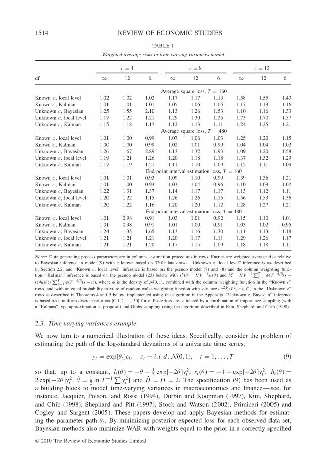
TABLE 1
Weighted average risks in time varying variances model
c = 4 c = 8 c = 12
df ∞ 12 6 ∞ 12 6 ∞ 12 6
Average square loss, T = 160Known c, local level 1.02 1.02 1.02 1.17 1.17 1.13 1.58 1.55 1.43Known c, Kalman 1.01 1.01 1.01 1.05 1.06 1.05 1.17 1.19 1.16Unknown c, Bayesian 1.25 1.55 2.10 1.13 1.26 1.53 1.10 1.16 1.33Unknown c, local level 1.17 1.22 1.21 1.29 1.30 1.25 1.73 1.70 1.57Unknown c, Kalman 1.15 1.18 1.17 1.12 1.13 1.11 1.24 1.25 1.21
Average square loss, T = 480Known c, local level 1.01 1.00 0.99 1.07 1.06 1.03 1.25 1.20 1.15Known c, Kalman 1.00 1.00 0.99 1.02 1.01 0.99 1.04 1.04 1.02Unknown c, Bayesian 1.26 1.67 2.89 1.13 1.32 1.93 1.09 1.20 1.58Unknown c, local level 1.19 1.21 1.26 1.20 1.18 1.18 1.37 1.32 1.29Unknown c, Kalman 1.17 1.19 1.21 1.11 1.10 1.09 1.12 1.11 1.09
End point interval estimation loss, T = 160Known c, local level 1.01 1.01 0.93 1.09 1.10 0.99 1.39 1.36 1.21Known c, Kalman 1.01 1.00 0.93 1.03 1.04 0.96 1.10 1.09 1.02Unknown c, Bayesian 1.22 1.31 1.37 1.14 1.17 1.17 1.13 1.12 1.11Unknown c, local level 1.20 1.22 1.15 1.26 1.26 1.15 1.56 1.53 1.36Unknown c, Kalman 1.20 1.22 1.16 1.20 1.20 1.12 1.28 1.27 1.21
End point interval estimation loss, T = 480Known c, local level 1.01 0.98 0.91 1.03 1.01 0.92 1.15 1.10 1.01Known c, Kalman 1.01 0.98 0.91 1.01 1.00 0.91 1.03 1.02 0.95Unknown c, Bayesian 1.24 1.35 1.65 1.13 1.16 1.30 1.11 1.13 1.18Unknown c, local level 1.21 1.21 1.21 1.20 1.17 1.11 1.29 1.26 1.17Unknown c, Kalman 1.21 1.21 1.20 1.17 1.15 1.09 1.18 1.18 1.11
Notes: Data generating process parameters are in columns, estimation procedures in rows. Entries are weighted average risk relativeto Bayesian inference in model (9) with c known based on 3200 data draws. “Unknown c, local level” inference is as describedin Section 2.2, and “Known c, local level” inference is based on the pseudo model (7) and (8) and the column weighting func-tion. “Kalman” inference is based on the pseudo model (23) below with sr
t (θ ) = H V −1st (θ ) and hrt = H V −1 ∑T
s=1 φ(T−4/5(s −t))ht (θ )/
∑Ts=1 φ(T−4/5(s − t)), where φ is the density of N(0, 1), combined with the column weighting function in the “Known c”
rows, and with an equal probability mixture of random walks weighting function with variances c2 S /T 2, c ∈ C , in the “Unknown c”rows as described in Theorems 4 and 5 below, implemented using the algorithm in the Appendix. “Unknown c, Bayesian” inferenceis based on a uniform discrete prior on {0, 1, 2, . . . , 50} for c. Posteriors are estimated by a combination of importance sampling (witha “Kalman”-type approximation as proposal) and Gibbs sampling using the algorithm described in Kim, Shephard, and Chib (1998).
2.3. Time varying variances example
We now turn to a numerical illustration of these ideas. Specifically, consider the problem ofestimating the path of the log-standard deviations of a univariate time series,
yt = exp[θt ]εt , εt ∼ i .i .d . N(0, 1), t = 1, . . . , T (9)
so that, up to a constant, lt (θ ) = −θ − 12 exp[−2θ ]y2
t , st (θ ) = −1 + exp[−2θ ]y2t , ht (θ ) =
2 exp[−2θ ]y2t , θ = 1
2 ln[T −1 ∑ y2t ] and H = H = 2. The specification (9) has been used as
a building block to model time-varying variances in macroeconomics and finance—see, forinstance, Jacquier, Polson, and Rossi (1994), Durbin and Koopman (1997), Kim, Shephard,and Chib (1998), Shephard and Pitt (1997), Stock and Watson (2002), Primiceri (2005) andCogley and Sargent (2005). These papers develop and apply Bayesian methods for estimat-ing the parameter path θt . By minimizing posterior expected loss for each observed data set,Bayesian methods also minimize WAR with weights equal to the prior in a correctly specified
© 2010 The Review of Economic Studies Limited

MULLER & PETALAS PARAMETER PATH IN UNSTABLE TIME SERIES MODELS 1515
model. It thus makes sense to use Bayesian inference as a benchmark for the WAR of the pathestimator described above. While the estimation of all models is based on the likelihood of(9), we also compute risk for data that is drawn from
yt = exp[θt ]
√df − 2
dfεt , εt ∼ i .i .d .student-t(df), df > 2, t = 1, . . . , T , (10)
so that the maintained model (9) is misspecified for df < ∞. Note that θt , the log-standarddeviation of yt , remains the pseudo-true parameter in (10) when estimating (9).
In addition to the path estimator based on the local level pseudo model (7) and (8) ofSection 2.2, we also consider inference based on a robustified pseudo model that does notreplace ht (θt ) by the constant H in (2), but by a kernel smoothed average of ht (θ). This pseudomodel leads to a somewhat more involved Kalman-smoother-based algorithm for obtaining anoptimal parameter path estimate described in the Appendix. The potential advantage is higherapproximation accuracy, as the smoother takes into account some low-frequency movementsin ht (θt ).
We compare WAR in two decision problems: (i) estimation of the parameter path undermean square error loss, so that for a path estimate {at }T
t=1, loss is given by T −1 ∑(θt − at )2 (andrisk becomes mean squared error averaged over t); (ii) estimation of an interval [al , ah ] for theend point of the parameter path θT , with loss equal to ah − al + 40 · 1[θT < al ](al − θT ) + 40 ·1[θT > au ](θT − au ) (so that a 10% increase in risk is equivalent to systematically reporting10% longer intervals with the same coverage probability, and with end points that are no closerto θT when θT falls outside the interval).2 Under the approximation discussed in Section 2.2(with p = k = 1 and {βt }T
t=1 = {θt }Tt=1), the best decisions are given by {at }T
t=1 = {θt }Tt=1
and, using Proposition 5.78 of Schervish (1995), [al , ah ] = [θT − 1.96√�t ,jj , θT + 1.96
√�t ,jj ],
respectively.WAR equals expected loss for data that is generated with parameters randomly drawn from
the weighting function. Table 1 reports relative WAR estimated in this way for the weightingfunction θ0 ∼ N(0, 100) and θt − θt−1 ∼ i .i .d .N(0, c2/HT 2) for c = 4, 8, 12 and T = 160, 480(think of 40 years of quarterly and monthly data, respectively). Under this weighting function,the median range of {θt }T
t=1 is approximately 1.1c/√
T , and 1.1c/√
T � 0.70 for c = 8 andT = 160, which compares with the estimated range of the log-standard deviation of the USfour-quarter growth rate of about 0.59 (cf. Table 1, Stock and Watson, 2002). By invertingthe QLR test statistic, Stock and Watson (1996) obtain median unbiased estimates for c forthe parameters of 76 univariate AR(6) models of US post-war macroeconomic monthly timeseries, and never find an estimate larger than 12. Cogley and Sargent (2005) estimate time-varying coefficients and volatility of a monetary VAR and report that this time variation wouldbe detected by a 5% level parameter stability test about 25% of the time, which roughlycorresponds to the columns with c = 4 in Table 1. This evidence suggests that the degree ofinstability implied by the weighting functions considered in Table 1 are moderate to large byan empirical standard.
Except for Monte Carlo error, the entries under “df = ∞, known c” must be larger thanunity by the small sample optimality of Bayesian inference in the correctly specified model.At the same time, the results of Section 3 show that these entries are approximately equal to1 for large sample sizes. For “unknown c”, the moderately lower risk of pseudo-model-basedinference relative to Bayesian inference in the correctly specified model with c = 4 seems to
2. The theoretical development in Section 3 assumes loss to be bounded. We computed WARs with truncatedloss functions and truncation point 40 times larger than the median loss, and found results very similar to thosereported in Table 1.
© 2010 The Review of Economic Studies Limited

1516 REVIEW OF ECONOMIC STUDIES
stem from a moderate downward bias in the estimated c induced by the robustification. Undermisspecification, Bayesian inference is no longer optimal by construction, and inference basedon robust pseudo models does relatively better. This effect is especially pronounced when cis unknown, since Bayesian inference rationalizes outliers generated by the student-t distur-bances by variation in θt , leading to an upward biased posterior for c, and a correspondingunder-smoothing of the parameter path. For very large instabilities c = 12, the simple algo-rithm of Section 2.2 has substantially larger WAR relative to Bayesian inference, but the morecomplicated Kalman pseudo model continues to provide quite accurate approximations.
In the Supplementary Materials,3 we report additional computations for true paths that areeither a linear trend or a step function with known or unknown break date. As expected, pathestimators that impose the correct parametric restriction have lower risk relative to the LocalLevel and Kalman smoother path estimators, at least if the magnitude of the instability is large.At the same time, in the single break model with small or moderate break (less than 6 standarddeviations of the full sample estimator θ ), the Local Level and Kalman estimators outperformestimators of the path that rely on a break date estimated by the least squares mean shift of|yt | or y2
t .
3. ASYMPTOTICALLY EFFICIENT INFERENCE IN UNSTABLETIME SERIES MODELS
We begin by introducing some additional notation and definitions. Consider a standard paramet-ric model for data YT = (yT ,1, . . . , yT ,T ) ∈ RmT in a sample of size T , a random vector definedon the complete probability space (F, F, P) , with parameter θ ∈ � ⊂ Rk , and known density∏T
t=1 fT ,t (θ ) with respect to some σ -finite measure μT . This form of likelihood arises naturallyin the “forecasting error decomposition” of models, where fT ,t (θ ) is the conditional likelihoodof yT ,t given FT ,t−1, where FT ,t ⊂ F is the σ -field generated by {yT ,s }t
s=1. In models withweakly exogenous components, fT ,t (θ ) can be decomposed into two pieces fT ,t (θ ) = f 1
T ,t (θ )f 2T ,t ,
where f 2T ,t captures the contribution of the evolution of weakly exogenous components and does
not depend on θ . If this is the case, only f 1T ,t (θ ) needs to be specified. Define lT ,t (θ ) = ln fT ,t (θ ),
sT ,t (θ ) = ∂lT ,t (θ )/∂θ , and hT ,t (θ ) = −∂sT ,t (θ )/∂θ ′. In the following definitions and conditions,we omit the dependence on T of FT ,t , lT ,t , sT ,t , hT ,t , and so forth, to enhance readability. Let[·] indicate the largest lesser integer function, let || · || denote the spectral norm, let “⊗” be theKronecker product, and let “
p−→” and “⇒” denote convergence in probability and convergencein distribution as T → ∞, respectively. Convergences of cadlag functions on the unit intervalare relative to the usual Billingsley (1968)-metric.
We assume the following condition on this model with true and stable parameter θ0.
Condition 1 (MEAS). The functions f 1T ,t : Rm × � → R are jointly measurable for t =
1, . . . , T .(DIFF) θ0 is an interior point of �, and in some neighbourhood �0 ⊆ � of θ0, lt is twice
continuously differentiable a.s. for t = 1, . . . , T .(ID) There exists η > 0 such that for all ε > 0 there exists K (ε) > 0 for which P (sup||θ−θ0||≥ε
T −1 ∑ sup||v ||<T −1/2+η ,θ+v∈�(lt (θ + v ) − lt (θ0)) < −K (ε)) → 1(LLLN) (i) For any decreasing ball BT around θ0, i.e. BT = {θ : ||θ − θ0|| < bT } for a
sequence of real numbers bT → 0, T −1 ∑Tt=1 supθ∈BT
||ht (θ ) − ht (θ0)|| p−→ 0, (ii) T −1 ∑Tt=1
||ht (θ0)|| = Op(1) and (iii) supλ∈[0,1]
∥∥T −1 ∑[λT ]t=1 ht (θ0) − ∫ λ
0 �(l )dl∥∥ p−→ 0 for some nonstochas-
tic matrix function � (possibly indexed by θ0), with �(λ) positive definite for all λ ∈ [0, 1].
3. Supplementary Materials are located on the ReStud website. See http://www.restud.org.uk/supplementary.asp
© 2010 The Review of Economic Studies Limited

MULLER & PETALAS PARAMETER PATH IN UNSTABLE TIME SERIES MODELS 1517
(MDA) {st (θ0), Ft } is a martingale difference array, there exists ε > 0 such that T −1 ∑Tt=1
E [||st (θ0)||2+ε |Ft−1] = Op(1) and supλ∈[0,1] ||T −1 ∑[λT ]t=1 E [st (θ0)st (θ0)′|Ft−1] − ∫ λ
0 �(l )dl ||p−→ 0.
Condition 1 is a set of fairly standard high-level assumptions on the “forecast error decom-position” part of the likelihood. (DIFF) assumes existence of two derivatives. (ID) is similar tothe global identification condition assumed in Schervish (1995, p. 436), somewhat strengthenedto ensure that even a slightly perturbed evaluation of the likelihood at parameter values differentfrom θ0 still yields a lower likelihood with high probability. (LLLN) is a Local Law of LargeNumbers for the second derivatives ht . Part (i) controls the average variability of the secondderivative ht as a function of the parameter. Part (iii) allows the information accrual to varyover the sample, and �(λ) describes the average information at time t = [λT ]. This allows, forinstance, accommodating regression models with a time trend t/T as regressor (the scaling by1/T ensures that the probability limit of T −1 ∑[λT ]
t=1 ht (θ0) remains Op(1) and positive definite).If ht (θ0), t = 1, . . . , T is positive semi-definite almost surely, part (ii) of (LLLN) is impliedby part (iii). (MDA) assumes the sequence of scores to constitute a martingale differencearray with slightly more than two conditional moments, with an average conditional varianceof �(λ) at time t = [λT ]. Whenever the relevant conditional moments exist, {st (θ0}, Ft } and{st (θ0)st (θ0)′ − ht (θ0), Ft } are martingale difference arrays by construction—see Chapter 6.2of Hall and Heyde (1980). Phillips and Ploberger (1996) and Li and Muller (2009) make verysimilar assumptions to (LLLN) and (MDA). Models with asymptotically stochastic information,such as unit root models, are not covered by Condition 1.
Now consider an unstable version of this parametric model, with time-varying parameterθt = θ + δt , t = 1, . . . , T , so that the density of the data YT becomes
fT (θ , δ) =T∏
t=1
fT ,t (θ + δt ), θ + δt ∈ � for t = 1, . . . , T (11)
where θ and δt are k × 1 and δ = (δ′1, . . . , δ′
T )′ ∈ RTk .4 Alternative estimators of {θ + δt }Tt=1, or
generally actions, are evaluated via a loss function LT : Rk × RTk × AT → [0, L] ⊂ R, wherethe action space AT is a topological space and LT is assumed Borel-measurable with respect tothe product sigma algebra on Rk × RTk × AT . (For reasons that will become apparent below,loss is also defined for parameter values outside �.) The bound L is finite and does not dependon T ; this assumption of bounded loss greatly facilitates the subsequent analysis. When the trueparameter evolution is {θ + δt }T
t=1 and action a ∈ AT is taken, the incurred loss is LT (θ , δ, a).A typical action could be an estimate of the entire parameter path, so that AT = �T , or anestimate of the parameter at a specific point in time, in which case AT = �. Decisions a aremeasurable functions from the data to AT . The risk of decision a given parameter evolution{θ + δt }T
t=1 is hence given as r(θ , δ, a) = ∫LT (θ , δ, a)fT (θ , δ)dμT , which in general depends on
δ and θ .Let QT be a measure on RTk , and let w : � → [0, ∞) be a Lebesgue probability density. For
each θ ∈ �, let VT (θ ) = {δ : δt + θ ∈ �∀t} ⊆ RTk . The WAR of decision a is then given by
WAR(a) =∫�
w (θ )∫VT (θ )
r(θ , δ, a)dQT (δ)dθ. (12)
4. In rational expectation models, the presence of time variation in θ potentially affects the model’s solution,and thus complicates the derivation of an appropriate likelihood compared to the corresponding model with stableparameters; see Fernandez-Villaverde and Rubio-Ramirez (2007) for one possible computationally intensive approach.
© 2010 The Review of Economic Studies Limited

1518 REVIEW OF ECONOMIC STUDIES
The weighting functions w and QT describe the importance attached to alternative true param-eter paths in the overall risk calculations; the weight function w attaches different weights tothe baseline value θ , and QT describes the weight on deviations from this baseline value. In theparameterization {θt }T
t=1 = {θ + δt }Tt=1, the average T −1 ∑ δt and θ are obviously not uniquely
identified. The same WAR criterion may thus be expressed by different choices of w and QT .The parameterization is useful because the weighting schemes analysed in this paper assumedifferent asymptotic properties of QT and w as follows.
Condition 2 (GS). The weight function QT is the distribution of {T −1/2G(t/T )}Tt=1, where
G is a k × 1 zero mean Gaussian semi-martingale on the unit interval with covariance kernelE [G(r)G(s)′] = κG (r , s). There exists a finite set of numbers τ = {0, τ1, . . . , τq} ⊂ [0, 1] suchthat ||∂2κG (r , s)/∂r∂s|| and ||∂2κG (r , s)/∂r2|| are bounded when r , s /∈ τ and r �= s, κG admitsbounded left and right derivatives with respect to r for all r = s ∈ [0, 1] \τ , and ||∂κG (r , s)/∂r ||is bounded for r ∈ [0, s)\τ and s ∈ τ .
(CNT) The weight function w does not depend on T and w is continuous at θ0.
Under Condition 2 (GS), the weight function QT focuses on persistent paths of relativelysmall variability, because Gaussian processes that satisfy the differentiability assumptions ontheir kernel are almost surely continuous for all s ∈ [0, 1]\τ by Kolmogorov’s continuitytheorem. This concentration on persistent parameter paths drives the derivation of the asymp-totic equivalence results below, and it is appealing in many applications, as parameter instabilityis typically thought of as a low-frequency phenomenon. As discussed in Section 2 above, a pop-ular choice in applied work has been the assumption that parameters vary as a Gaussian randomwalk, which may be achieved by setting G equal to G(·) = ϒ1/2W (·), where W is a k × 1 stan-dard Wiener process. Random walk parameter variability that only occurs in, say, the first half ofthe sample is achieved by letting G(s) = 1[s ≤ 1/2]ϒ1/2W (s) + 1[s > 1/2]ϒ1/2W (1/2). Anassumption of slowly mean reverting parameters can be expressed by letting G be a stationaryOrnstein–Uhlenbeck process, more weight on smoother paths by letting G be an integratedBrownian motion G(s) = ∫ s
0 W (r)dr , etc. Condition 2 also accommodates piece-wise constantpaths with finitely many jumps, as in the multiple breaks literature, although specification ofQT requires knowledge of the break dates.
Under Condition 2 (GS), the WAR criterion (12) focuses on parameter paths whose variabil-ity is of order of magnitude T −1/2. This choice is motivated by a desire to develop proceduresthat work well when there is relatively little information about the parameter path. For parame-ter paths of fixed magnitude and persistence, larger samples naturally contain more information,as more adjacent observations can be used to pinpoint the value of the slowly varying param-eter at a given date. The sample-size-dependent choice of the magnitude of {δt } under QT
counteracts this effect, making the estimation of the form of the scaled parameter variation{T 1/2δt } difficult even asymptotically. In this way, the asymptotic arguments derived belowbased on the sequence of weights as described in Condition 2 (GS) become hopefully rele-vant to the small sample problem where there is in fact little information about the parameterevolution. At the same time, Condition 2 (CNT) assumes w not to depend on the sample size,reflecting a “global” uncertainty about the baseline level of the time-varying parameter path.With the continuity at θ0, the weight function becomes asymptotically flat in the T −1/2 localneighbourhood around θ0, so that sample information dominates inference about the baselinevalue.
The order of magnitude T −1/2 for δt under Condition 2 (GS) corresponds to the localneighbourhood in which efficient stability tests have non-trivial asymptotic power. The null
© 2010 The Review of Economic Studies Limited
MULLER & PETALAS PARAMETER PATH IN UNSTABLE TIME SERIES MODELS 1519
hypothesis of a stability test is that the parameter path {θt }Tt=1 = {θ + δt }T
t=1 is con-stant, i.e.
H0 : δt = 0 for t = 1, . . . , T (13)
against the alternative that the parameter is time varying. For the development of optimal param-eter stability tests, it makes sense to restrict the parameter paths under the alternative such thatthe difference to the corresponding stable model is the time variability of the path, rather thana different average value of the path. The appropriate restriction is achieved by the multivariateGaussian measure Q∗
T of {T −1/2(G(t/T ) − (∑T
s=1 �(s/T ))−1 ∑Ts=1 �(s/T )G(s/T ))}T
t=1. Wheninformation accrual is constant, that is �(s) = H for all s ∈ [0, 1], then the restriction amountsto a demeaning of δt , such that
∑δt = 0 a.s. under Q∗
T . In the general case, the restrictionforces
∑�(t/T )δt = 0, so that the information weighed parameter path deviations sum to
zero, just as in the efficient tests derived by Andrews and Ploberger (1994). Intuitively, amodel with time-varying parameter is closest to the stable model with a parameter that is theinformation-weighted average of the parameter path.
Possibly randomized parameter stability tests ϕT are measurable functions from the datato the interval [0, 1], where ϕT (yT ) indicates the probability of rejecting the null hypothesisof parameter stability when observing YT = yT . Tests of the same size can then usefully becompared by considering their weighted average power
WAP (ϕT ) =∫VT (θ0)
∫fT (θ0, δ)ϕT dμT dQ∗
T (δ) (14)
similar to Andrews and Ploberger (1994). While θ0 is typically unknown, we show below thatthere exists a feasible test ϕ∗
T that asymptotically maximizes this weighted average power.With the weighting of parameter paths specified as the distribution of a Gaussian process,
the problem of finding WAR-minimizing actions essentially becomes a non-linear smoothingexercise. The WAR-minimizing decision is to choose the action a that minimizes∫
�w (θ )
∫VT (θ ) fT (θ , δ)LT (θ , δ, a)dQT (δ)dθ∫
�w (θ )
∫VT (θ ) fT (θ , δ)dQT (δ)dθ
(15)
for each data realization YT = yT . With the weighting functions normalized to integrate tounity, this is simply Bayes Rule for minimizing Bayes risk (15), which can be interpreted asfinding the action that minimizes the posterior expected loss, i.e. loss integrated with respectto the posterior distributions of (θ , δ) under a prior for (θ , δ) that corresponds to the weightsin Condition 2.
A large literature has developed around numerically finding exact posterior distributionsin non-linear filtering/smoothing problems, often by Monte Carlo simulation techniques, asreviewed in the introduction. This paper complements this research by an asymptotic analysis.First, this yields a deeper theoretical understanding of the link between the estimation testingproblems. Second, the asymptotic analysis suggests a computationally simple and asymptot-ically efficient procedure for choosing the risk-minimizing action. Third, unlike the BayesRule computed numerically from (15), the approximately risk-minimizing action can easily beappropriately modified for potentially misspecified models.
Note that Condition 1 makes assumptions about the stable model only, that is, on itsbehaviour when the parameter path is constant. Clearly, with a focus on the problem of esti-mating the parameter path, we need to argue for the accuracy of approximations also whenthe true data-generating process has time-varying parameters. In general, most models with
© 2010 The Review of Economic Studies Limited
1520 REVIEW OF ECONOMIC STUDIES
time-varying parameters generate non-stationary data, to which standard asymptotic results arenot easily applicable. In a vector autoregressive regression model, for instance, parameter insta-bilities lead to highly complicated interactions between the evolution of the lagged variablesand the unstable parameters. Our approach is thus to derive asymptotic results for unstablemodels as an implication of the contiguity of models with time-varying parameters of orderT −1/2 to the corresponding stable model, similar to Andrews and Ploberger (1994), Phillips andPloberger (1996), Elliott and Muller (2006), and Li and Muller (2009). The following Lemmafollows from Lemma 1 of Li and Muller (2009) and the additional discussion in their appendix.
Lemma 1. Let π0 : [0, 1] → Rk be a piece-wise continuous function with at most a finitenumber of discontinuities and left and right limits everywhere. Under Condition 1, the sequenceof densities
∏Tt=1 fT ,t (θ0, T −1/2π0(t/T )) is contiguous to the sequence fT (θ0, 0). Furthermore,
under Conditions 1 and 2, the two sequences of densities∫VT (θ0) fT (θ0, δ)dQT (δ)/
∫VT (θ0) dQT (δ)
and∫VT (θ0) fT (θ0, δ)dQ∗
T (δ)/∫VT (θ0) dQ∗
T (δ) are contiguous to the sequence fT (θ0, 0).
The main result of the paper is the following Theorem.
Theorem 1. Let the sequence of positive definite matrices {ht }Tt=1 = {hT ,t }T
t=1 satisfy
supλ∈[0,1]
∥∥∥∥∥T −1[λT ]∑t=1
ht −∫ λ
0�(s)ds
∥∥∥∥∥ p−→ 0 (16)
in the stable model with parameter θ0.(i) Consider WAR (12) of alternative decisions a under Condition 2. If Condition 1 and (16)
hold for almost all θ0 in the support of w , and for each YT = yT , the decision a∗ minimizesWAR with weights as in Condition 2 or a flat weighting of θ and the weight function QT on δ
in the pseudo model
st (θ ) + ht θ = ht (δt + θ ) + νt , νt ∼ independent N(0, ht ), t = 1, . . . , T , (17)
then for all a, lim infT→∞[WAR(a) − WAR(a∗)] ≥ 0.(ii) For any YT = yT , let Q∗
T be the distribution of {T −1/2G(t/T ) − T −1/2(∑T
s=1 hs )−1 ∑Ts=1
hs G(s/T )}Tt=1 (induced by G), and let ϕ∗
T be a test of (13) of asymptotic level α that maximizesweighted average power with respect to the weighting function Q∗
T in the pseudo model
st (θ ) = htδt + νt , νt ∼ independent N(0, ht ), t = 1, . . . , T . (18)
Then under Conditions 1 and 2, for any other test ϕT of (13) of asymptotic level α, lim infT→∞[WAP (ϕ∗
T ) − WAP (ϕT )] ≥ 0.(iii) Under Condition 1, the total variation distance between the posterior distribution of
(θ , δ) in model (11) with priors as in Condition 2 and the posterior distribution of (θ , δ) in thepseudo model (17) with either the same priors or with a flat prior on θ and prior QT on δ
converges in probability to zero in both the stable model with parameter θ0 and any unstablemodel that satisfies the condition of Lemma 1.
Theorem 1 asserts that asymptotically efficient decisions and tests are obtained from com-bining the sample information from pseudo models (17) and (18), respectively, with theweighting of Condition 2. Since both of these are Gaussian, the resulting distribution canbe computed explicitly. Let e be the Tk × k matrix e = (Ik , . . . , Ik )′, Dh = diag(h1, . . . , hT ),
© 2010 The Review of Economic Studies Limited

MULLER & PETALAS PARAMETER PATH IN UNSTABLE TIME SERIES MODELS 1521
�δ = Eδ[δδ′], where Eδ denotes integration of δ ∼ QT of Condition 2, K = �δ(Dh�δ + ITk )−1,s = (s1(θ)′, . . . , sT (θ)′)′ and
� = K + (ITk − KDh )e(e′Dh e − e′Dh KDh e)−1e′(ITk − Dh K ). (19)
Note that with δ ∼ N(0,�δ) and the measurements Xt = htδt + νt , νt ∼ independent N(0, ht ),t = 1, . . . , T , the distribution of δ conditional on the measurements X = (X ′
1, . . . , X ′T ) and Dh
is δ|(X, Dh ) ∼ N(K X, K ). The second term in the definition of � results from the uncertaintyconcerning the baseline value θ. The matrix � remains the same if �δ is substituted by thecovariance matrix of δ under Q∗
T , as defined in Theorem 1 (ii).5
Theorem 2. Let � be the distribution N(eθ + �s,�).(i) The decision a∗ that minimizes expected risk relative to the distribution eθ + δ ∼ � for
each YT = yT minimizes WAR in the pseudo model (17) with a flat weighting on θ.
(ii) A test that rejects for large values of s′�s is the optimal stability test in the pseudomodel (18), and under Conditions 1 and 2
s′�s ⇒ 2 ln
(EG exp[
∫ 10 G∗(s)′�(s)1/2dW ∗(s) − 1
2
∫ 10 G∗(s)′�(s)G∗(s)ds]
EG exp[− 12
∫ 10 G∗(s)′�(s)G∗(s)ds]
)
under the null hypothesis, where G∗(s) = G(s) − (∫ 1
0 �(λ)dλ)−1∫ 1
0 �(λ)G(λ)dλ, the standardk × 1 Wiener process W ∗ is independent of G and EG denotes integration with respect to theprobability measure of G.
(iii) The posterior distribution of eθ + δ under a flat prior on θ in the pseudo model (17) isgiven by �.
Comments:1. Part (i) of Theorem 1 establishes that for arbitrary bounded loss functions, the decisionthat minimizes WAR in the Gaussian pseudo model (17) is also asymptotically optimal in thetrue model. As shown in part (i) of Theorem 2, this amounts to finding the risk-minimizingaction relative to a multivariate Gaussian distribution for the parameter path. Note that lossmay be defined arbitrarily (subject to the bound L) for parameter values outside �, allowingthe problem in the pseudo model to be made entirely spherical. For the wide range of boundedbowl-shaped loss functions for which one would choose the posterior mean in a Gaussianmodel, an asymptotically efficient parameter path estimator is hence given by eθ + �s byAnderson’s (1955) Lemma. Note that such loss functions include those that consider a weightedaverage of symmetric losses incurred by estimation errors in the parameter value, such as
LT (θ , δ, a) =T∑
t=1
qT ,t L0(T (θ + δt − at )′WL(θ + δt − at )) (20)
where a = (a ′1, . . . , a ′
T )′ ∈ RTk , inft≤T qT ,t ≥ 0,∑T
t=1 qT ,t = 1, WL is a non-negative definitek × k matrix and L0 : [0, ∞) → [0, L] is a monotonically increasing function with L0(0) = 0.The scaling by T in (20) ensures that the loss does not become trivial as T → ∞ even for goodpath estimators, although Theorems 1 and 2 remain true without this scaling. This class of loss
5. This follows from Theorem 2 (i): combined with the flat weighting on θ , all weighting functions for δt thatimply the same weighting for {δt − T −1 ∑T
s=1 δs }Tt=1 yield the same overall weighting function for {θ + δt }T
t=1.
© 2010 The Review of Economic Studies Limited

1522 REVIEW OF ECONOMIC STUDIES
functions (20) contains the special case where one only cares about the parameter at time T ,i.e. qT ,T = 1 and qT ,t = 0 for all t < T , which arises naturally in a forecasting problem.
For more general losses and decision problems, the asymptotically efficient decision canstill be obtained by implementing the efficient decision in the Gaussian pseudo model. Thistypically represents a very substantial computational simplification.
2. Part (ii) of Theorems 1 and 2 spell out the implications of the approximation for efficienttests of the null hypothesis of parameter stability (13). Part (i) of Theorem 2 shows thatunder symmetric loss, the asymptotically efficient parameter path estimator is eθ + �s with anasymptotic uncertainty described by a zero mean multivariate normal with covariance matrix�. The asymptotically efficient test statistic s′�s = (�s)′�+(�s), where �+ denotes a generalinverse, is recognized to be of the usual Wald form: efficient instability tests are based ona quadratic form in the efficient estimator of the instability. Efficient estimation and testingin (potentially) unstable models are hence unified in one framework. This ensures coherencebetween the stability test and the path estimator, as s′�s can be large only if the path estimatoreθ + �s shows substantial variation.
3. Part (iii) of Theorems 1 and 2 describe the approximation result in Bayesian terms: theposterior distribution of the parameter path eθ + δ comes arbitrarily close to the Tk -dimensionalmultivariate normal distribution N(eθ + �s,�). This is a considerably stronger statement thana convergence in distribution of, say, the posterior of T 1/2δ[·T ] viewed as an element of thespace of cadlag functions on the unit interval. With G(s) = 0, so that �δ = K = 0, � becomes� = e(e′Dh e)−1e′, and one recovers the standard result that the posterior distribution of θ
converges to N(θ , T −1H −1) where H = T −1 ∑ htp−→ ∫
�(λ)dλ, the average information.In practice, part (iii) of Theorem 1 is useful for Bayesian analyses, as it provides a simple
way to compute approximation to the posterior of the unstable parameter path. Even if theexact small sample posterior is required, the approximation of Theorem 1 might be accurateenough for a simple importance sampling algorithm to succeed.
4. The asymptotic distribution of the test statistic s′�s is provided in Theorem 2 (ii).This distribution is non-standard and depends on the weighting function G and the evolutionof the information �. Even with � known, a simulation based on this expression is quitecumbersome due to the integration over the measure of G . Theorem 2 (ii) is still useful as itshows the existence of an asymptotic distribution. It thus suffices to consider a computationallyconvenient stable model that has the same asymptotic distribution, such as the stable Gaussianlocation model Xt = htθ + Zt , t = 1, . . . , T with Zt independent and distributed N(0, ht ). Thelimiting distribution of Z′�Z with Z = (Z ′
1, . . . , Z ′T )′ and Zt = Zt − ht (
∑Ts=1 hs )−1 ∑T
s=1 hsZs
is therefore the same as the asymptotic null distribution of s′�s, for {ht } drawn both from thestable model and under all local alternatives for which Lemma 1 implies (16) to also hold.6
Asymptotically justified critical values of the test statistic s′�s might hence be obtained byconsidering the empirical distribution of sufficiently many draws from the distribution of Z′�Z,similar to the approach of Hansen (1996).
5. The approximation results in Theorems 1 and 2 hold for any choice of positive definitesequences {ht } that satisfy (16) in the stable model: in the limit, it is only the average behaviourof ht that determines the properties of the pseudo models (17) and (18). In particular, with�(s) = H a constant function, this result allows us to choose ht time invariant ht = H for anyconsistent estimator H of H , as exploited by the algorithm of Section 2. Without the assumptionof a constant �, it makes sense to set ht equal to a standard non-parametric estimator of �(s),
6. Formally, this follows from replacing s by Z in the derivation of the asymptotic null distribution inTheorem 2 (ii).
© 2010 The Review of Economic Studies Limited

MULLER & PETALAS PARAMETER PATH IN UNSTABLE TIME SERIES MODELS 1523
such as a kernel-smoothed average of ht (θ) as studied in Robinson (1989). Lemma 3 (vi) in theAppendix shows that ht = ht (θ), and thus for continuous �(s), also kernel-smoothed averageswith bandwidth of order T −1/5, satisfy (16) under Condition 1. As explained in Section 2.2,the smoothing extracts the pertinent low-frequency properties of �(s) without imposing anaccurate quadratic approximation of the log-likelihood for each t . Pronounced instabilities canalso lead to effectively time-varying �(s), as in the example of Section 2.3; so choosing ht timevarying in this fashion might improve approximation accuracy even in models where formally�(s) = H .
6. For certain applications, it makes sense to make the scale of the weighting function in theestimation (12) and testing problems (14) a function of the information �. In a testing context,for instance, it is often attractive to choose G such that alternatives that are equally difficultto detect receive a similar weight, as in Wald (1943) and, conditional on the break date, inAndrews and Ploberger (1994). Typically, of course, � is unknown, and needs to be estimatedfrom the data. Optimal decisions and tests from the pseudo models (17) and (18) with respectto an estimated weighting function generally continue to be asymptotically optimal decisions interms of (12) and (14), i.e. with respect to the data-independent weighting functions describedin Condition 2.
Theorem 3. Suppose {�T ,t }Tt=1 are non-singular k × k statistics such that supt≤T ||�T ,t −
Ik || p−→ 0 and∑T
t=2 ||�T ,t − �T ,t−1|| p−→ 0 in the stable model with parameter θ0. Then part(ii) of Theorem 1 also holds for Q∗
T replaced by the distribution of {T −1/2�T ,t G(t/T ) − T 1/2
(∑T
s=1 hs )−1 ∑Ts=1 hs�T ,sG(s/T )}T
t=1 (induced by G). Furthermore, if supθ∈�,δ∈RTk ,a∈AT|LT (θ ,
diag(�T ,1, . . . ,�T ,T )δ, a) − LT (θ , δ, a)| → 0 for all sequences {�T ,t }Tt=1 satisfying supt≤T ||�T ,t
− Ik || → 0 and∑T
t=2 ||�T ,t − �T ,t−1|| → 0 as T → ∞, then also part (i) of Theorem 1 holdsfor QT replaced by the distribution of {T −1/2�T ,t G(t/T )}T
t=1 (induced by G).
In a typical application of Theorem 3, suppose one aims at computing the asymptoti-cally efficient test for a Condition 2 weighting function with G(·) = c�
−1/2W (·), where c
is a known scalar constant, but the average information � = ∫ 10 �(λ)dλ is not known. Then
Theorem 3 shows that this test may be computed from the pseudo model (18) with an estimated
weighting function that corresponds to the distribution of c�−1/2
W (·) = c�−1/2
�1/2
G(·), i.e.based on the statistic s′�s where �δ in the definition (19) of � has i , j -th k × k block equal
to T −2c2 ∑min(i ,j )t=1 �
−1, as long as �
p−→� under θ0 stable. In the more general case whereG(·) = R(·)G0(·) with G0 a known Gaussian process and R : [0, 1] → Rk×k an unknown fixedand nonsingular matrix function, Theorem 3 requires beyond consistency that the scaled esti-mation error �T ,t = RT ,t R(t/T )−1 is smooth by imposing
∑Tt=2 ||�T ,t − �T ,t−1|| p−→ 0. This
condition is typically satisfied for parametric estimators of R when R is of bounded variation,such as, for example, when R is a linear trend of unknown slope or when R is a step functionwith known step locations.
Moreover, optimal decisions from the pseudo model typically retain their WAR (12) opti-mality under such estimated weights, such as the path estimator eθ + �s under the class ofloss functions (20) when L0 is continuous. The restriction of the loss functions in the secondclaim of Theorem 3 is necessary to rule out a somewhat pathological focus of LT on the scaleof the weighting function for δ.7
7. For example, with G(s) = W (s) and �T ,t = (1 + T −1/4)Ik , LT (θ , δ, a) = (T 1/2tr(T∑
(�δt )(�δt )′ − Ik ))2 ∧1, limT→∞ EδLT (θ , δ, a) �= limT→∞ EδLT (θ , (1 + T −1/4)δ, a).
© 2010 The Review of Economic Studies Limited

1524 REVIEW OF ECONOMIC STUDIES
7. For some purposes, it makes sense to consider weighting functions that are more agnosticabout the magnitude and/or form of the parameter instability than is possible under Condition 2.One way to achieve this without foregoing the computational advantages of a Gaussian weight-ing function is to consider weighting functions (or priors) for δ that are a weighted average ofdistributions of different Gaussian processes. The following Theorem shows how parts (i) and(iii) of Theorems 1 and 2 need to be adapted in the case of such a finite mixture.
Theorem 4. Let Gi , i = 1, . . . , nG be processes satisfying Condition 2 (GS). If QT is thedistribution of the mixture of {T −1/2Gi (t/T )} with mixing probabilities pi , then parts (i) and (iii)of Theorems 1 and 2 hold with � replaced by the mixture of nG multivariate normal distributionsN(eθ + �i s,�i ) with mixing probabilities proportional to
wi = pi |Dh�δ(i ) + ITk |−1/2|e′Dh e − e′Dh Ki Dh e|−1/2 exp[ 12 s′�i s], i = 1, . . . , nG , (21)
where Ki , �δ(i ), and �i are defined as K , �δ , and � in (19) with �δ replaced by �δ(i ), thecovariance matrix of T −1/2(Gi (1/T )′, Gi (2/T )′, . . . , Gi (1)′)′ for i = 1, . . . , nG .
Theorem 4 is a simple consequence of the fact that the Gaussian pseudo model (17) remainsan accurate approximation of the sample information for each of the nG weighting functions,such that the likelihood ratios can be explicitly computed. The WAR-minimizing parameterpath estimator under mixture weightings generally depends much more on the loss functionthan in the single Gaussian process case, as mixtures of normal distributions are not generallysymmetric around their mean. Under truncated quadratic loss (20) with L0(x ) = min(x , L), theWAR-minimizing path estimator converges to
∑nGi=1 wi�i s/
∑nGi=1 wi as L → ∞.
8. So far we assumed that the model in Condition 1 is correctly specified. As demonstratedby Huber (1967) and White (1982), in misspecified models maximum likelihood estimators areconsistent for the pseudo-true parameter value that minimizes the Kullback–Leibler divergenceof the true model from the maintained model. This pseudo-true parameter value sometimesremains the natural object of interest as, for instance, in exponential models with correctlyspecified mean (cf. Gourieroux, Monfort, and Trognon, 1984). We now discuss a modificationof the pseudo model (17) such that, under some conditions, the best decision about the pseudo-true parameter path in a misspecified model yields the same asymptotic risk as the best decisionin a corresponding correctly specified model.
Suppose the evolution of the pseudo-true parameter through time is θt = θ0 + T −1/2π0(t/T ),and let st = st (θ ) and ht = ht (θ) be the scores and Hessians in the misspecified model. Understandard primitive assumptions, by the usual Taylor approximations, one would typically findthat
T −1/2[·T ]∑t=1
st ⇒ J (·) −∫ ·
0�(λ)dλ
(∫ 1
0�(λ)dλ
)−1
J (1),
T 1/2(θ − θ0) ⇒(∫ 1
0�(λ)dλ
)−1
J (1)
and
T −1[·T ]∑t=1
htp−→∫ ·
0�(λ)dλ,
© 2010 The Review of Economic Studies Limited

MULLER & PETALAS PARAMETER PATH IN UNSTABLE TIME SERIES MODELS 1525
where
J (s) =∫ s
0V (λ)1/2dW (λ) +
∫ s
0�(λ)π0(λ)dλ (22)
with V : [0, 1] → Rk×k and � : [0, 1] → Rk×k positive definite, non-stochastic matrix func-tions. See, for instance, Andrews (1993) and Li and Muller (2009) for primitive conditions thatinduce such convergences. The matrix V (s) is the average long-run variance of the scores st (θ0)at the time t = [sT ], which in a misspecified model is not in general equal to the average of theHessians �(s). The pseudo model (17) based on st , θ and ht directly thus behaves differentlythan the pseudo model of any correctly specified model, even asymptotically. Note, however,that if we premultiply the scores and Hessians by �(t/T )V (t/T )−1, we obtain a long-run vari-ance for �(t/T )V (t/T )−1st (θ0) of �(s)V (s)−1�(s) at time t = [sT ], which coincides with thelocal average of �(t/T )V (t/T )−1ht . This adjustment is the time-varying parameter analogueto the sandwich pseudo model suggested in Muller (2009) for Bayesian inference in stablemisspecified models.
Condition 3. In the misspecified model with parameter path equal to θt = θ0 +T −1/2π0(t/T ), there exist sequences of invertible k × k matrices {�t }T
t=1 and {Vt }Tt=1 such that
with srt = �t V
−1t st − T −1 ∑T
s=1 �s V −1s ss and θ r = θ + (
∑Tt=1 �t V
−1t ht )−1 ∑T
t=1 �t V−1
t st , wehave
T −1/2[·T ]∑t=1
s rt ⇒ J r (·) −
∫ ·
0�(λ)dλ
(∫ 1
0�(λ)dλ
)−1
J r (1)
and
T 1/2(θ r − θ0) ⇒(∫ 1
0�(λ)dλ
)−1
J r (1),
where
J r (s) =∫ s
0�(λ)1/2dW (λ) +
∫ s
0�(λ)π0(λ)dλ
and �(s) = �(s)V (s)−1�(s). Further, there exist matrices {h rt }T
t=1 such that
supλ∈[0,1]
∥∥∥∥∥T −1[λT ]∑t=1
h rt −
∫ λ
0�(s)ds
∥∥∥∥∥ p−→ 0.
The “robustified” estimator θ r and partial sums of the scores s rt and Hessians h r
t of Con-dition 3 behave just like the maximum likelihood estimator and partial sums of the scoresand Hessians would in a correctly specified model with average Fisher Information at timet = [sT ] equal to �(s) = �(s)V (s)−1�(s). This suggests that asymptotically, best decisions inthe robustified pseudo model
s rt + h r
t θr = h r
t (δt + θ ) + νt , νt ∼ independent N(0, h rt ), t = 1, . . . , T , (23)
have the same risk as best decisions in a correctly specified model with this Fisher Information.At the same time, if the model ends up being correctly specified, then �(s) = V (s) by theinformation equality, and θ r and partial sums of s r
t and h rt have the same asymptotic properties
as the original θ , st and ht .
© 2010 The Review of Economic Studies Limited

1526 REVIEW OF ECONOMIC STUDIES
In general, for Condition 3 to follow from the weak convergences mentioned above, �t andVt must be sufficiently accurate estimators of �(t/T ) and V (t/T ). Clearly, the constructionof appropriate estimators is the more difficult the less is known about the variability of �(·)and V (·). In the important special case of constant �(s) = H and V (·) = V , it suffices toset �t = H and Vt = V for any consistent estimators (H , V ) of (H , V ) (and in this case,θ r = θ and one possible choice for h r
t is h rt = S −1 = H V −1H ). Typically, the estimators H =
T −1 ∑Tt=1 ht and, as long as st (θ0) is serially uncorrelated in the stable misspecified model, V =
T −1 ∑Tt=1 st s ′
t are consistent, whereas if the misspecification leads to potentially autocorrelatedst (θ0), one needs to apply a standard long-run variance estimator to the scores {st }T
t=1. See Liand Muller (2009) for a discussion of possible primitive conditions for Condition 3.
Theorem 5. Consider a correctly specified model satisfying Condition 1 and parameterpath equal to θt = θ0 + T −1/2π0(t/T ), where π0 satisfies the conditions of Lemma 1, and leta∗ be the decision that, for each draw, minimizes expected risk relative to the distribution of� ∼ N(eθ + �s,�). Similarly, consider a potentially misspecified model satisfying Condition 3,and let ar∗ be the decision that, for each draw, minimizes expected risk relative to the distributionof �r ∼ N(eθ r + �r sr ,�r ), where sr is the Tk × 1 vector of stacked scores {s r
t }Tt=1, and �r is
constructed as � in (19) with ht replaced by hrt .
(i) Let a∗(�T ) be the action that minimizes expected risk relative to the Tk × 1 multivariatedistribution �T , and define π0 = (π0(1/T )′, . . . ,π0(T/T )′)′. If the common loss function LT issuch that
LT (θ0, π0, a∗(�1T )) − LT (θ0, π0, a∗(�2T )) → 0 (24)
whenever the total variation distance between the two Tk × 1 normal distributions �1T and �2T
converges to zero, then the difference between the sampling distributions of LT (θ0, π0, a∗) in thecorrectly specified model and LT (θ0, π0, a r∗) in the potentially misspecified model converges tozero in the Prohorov metric.
(ii) If (24) is strengthened to hold whenever the total variation distance between the twomixtures of nG normal distributions �1T and �2T converges to zero, then the conclusion of part(i) also applies with � replaced by the mixture distribution of Theorem 4, and �r defined asthe analogous mixture based on θ r , s r
t and hrt in the place of θ , st (θ) and ht .
(iii) The test statistics s′�s and sr ′�r sr have the same asymptotic distribution.
Theorem 5 formalizes the link between best inference based on the pseudo model in amisspecified model using the robustified statistics of Condition 3, and best inference based onthe pseudo model in a corresponding correctly specified model. The key assumption (24) forpart (i) is that similar multivariate normal distributions �1T and �2T induce best actions ofsimilar loss. This holds, for instance, for the loss function (20) as long as L0 is continuous.Under this assumption, the sampling distribution of the losses in these two models is asymp-totically identical, which—given that the loss is assumed bounded—also implies identical(frequentist) risk of the best decisions a∗ and a r∗. Thus, from a decision theoretic perspective,ignoring the misspecification is not costly in the sense that one still obtains inference of thesame asymptotic quality as in the corresponding correctly specified model. Similarly, part (iii)shows that the test statistic sr ′�r sr has the same asymptotic distribution as s′�s does in thecorresponding correctly specified model, and thus the same local power. In particular, if Con-dition 3 holds for π0(·) = 0, one may simulate the null distribution by many draws of Zr ′�r Zr
with Zr = (Z r ′1 , . . . , Z r ′
T )′, Z rt = Z r
t − h rt (∑T
s=1 h rs )−1 ∑T
s=1 h rs Z r
s and Zt independent N(0, h rt )
pseudo random variables, as discussed in Comment 4.
© 2010 The Review of Economic Studies Limited

MULLER & PETALAS PARAMETER PATH IN UNSTABLE TIME SERIES MODELS 1527
It is easy to see that these correspondences do not hold in general without the robustificationdetailed in Condition 3 and, in analogy to the formal results in Muller (2009), one would expectthat asymptotic risk is generally smaller in the robustified pseudo model. The reason is thatunder misspecification, both the original likelihood and uncorrected pseudo model (17) conveya misleading account of the sample information about the pseudo-true parameter, as the varianceof partial sums of st is different from the partial sum behaviour of the Hessians ht . Wheneverthe optimal action depends on the variance �r , one therefore should obtain lower asymptoticrisk decisions from the robustified model. What is more, if the weighting function (or prior)averages over alternative Gaussian processes as in Theorem 4, then a Bayesian or uncorrectedpseudo model (17) will in general lead to biased estimation of the magnitude of the parametertime variation, as the variability of st is mistakenly judged relative to ht . Inference based on therobustified pseudo model (23) is thus not only more convenient computationally compared to afully fledged Bayesian analysis, but also provides more reliable inference about the pseudo-trueparameter path in misspecified models.
9. Much applied work is based on the special case where the prior or weighting functionof a time-varying parameter is a Gaussian random walk, such that G(·) = ϒ1/2W (·) for somepositive semidefinite matrix ϒ and standard Wiener process W ; see the citations in Section 2.The Markovian structure of the Wiener process enables the application of an iterative Kalmansmoothing algorithm. We provide such an algorithm in the Appendix, which also takes careof the impact of the flat weighting of θ in the smoothing, along similar lines as Jong (1991),and enables computation of the statistics appearing in Theorems 2, 4, and 5 without matrixcomputations of dimension Tk × Tk .
The algorithm described in Section 2 of this paper exploits the additional computationalsimplifications when h r
t = S −1, t = 1, . . . , T and ϒ = c2Sβ , where Sβ is the upper left p × pblock of S .8 By Theorem 3, this choice of ϒ minimizes asymptotic WAR for the weightingfunction induced by ϒ = c2H −1
β for most loss functions in a correctly specified model with
�(s) = H as long as Sβ
p−→ H −1β , where H −1
β is the upper left p × p block of H −1.10. A number of previous papers have considered parameter stability tests against random
walk-type alternatives: Nyblom (1989) derives locally best tests against general martingalevariability in the parameters for general likelihood models, Shively (1988) considers smallsample tests in a linear regression model, and Elliott and Muller (2006) derive asymptotic resultsfor point optimal parameter instability tests in linear regression models for a class of weightingfunctions that includes the Gaussian random walk case. The contribution of Theorems 1, 2,and 5 with respect to this literature is the generalization of the point optimal tests to general,potentially misspecified likelihood models, including non-stationary models with, say, a timetrend. Under the assumption of correct misspecification, the degree of generality of the resultshere concerning parameter stability tests is similar to those of Andrews and Ploberger (1994),but the focus there is on parameters that shift at unknown dates, which leads Andrews andPloberger (1994) to consider weighting functions that are a continuous mixture of piece-wiseconstant parameter paths with Gaussian shifts.
Elliott and Muller (2006) show that efficient tests for a Gaussian random walk in theparameters and efficient tests for a single break at unknown date have asymptotic power thatis roughly comparable no matter what the true alternative is; the efficient tests for the Gaus-sian random walk have the advantage that they avoid the need for trimming the break dates
8. The algorithm in Section 2.2 stems from combining our results with those of Elliott and Muller (2006):applying the matrix identity (A5) in the Appendix, �r becomes (IT − Gc ) ⊗ Sβ with Gc defined in Elliott and Muller(2006), and the expressions for qLL(c) = −sr ′�r sr , wi and κt in Section 2.2 follow.
© 2010 The Review of Economic Studies Limited
1528 REVIEW OF ECONOMIC STUDIES
away from the beginning and end of the sample, and their computational convenience, at leastcompared to efficient tests for more than one potential break.
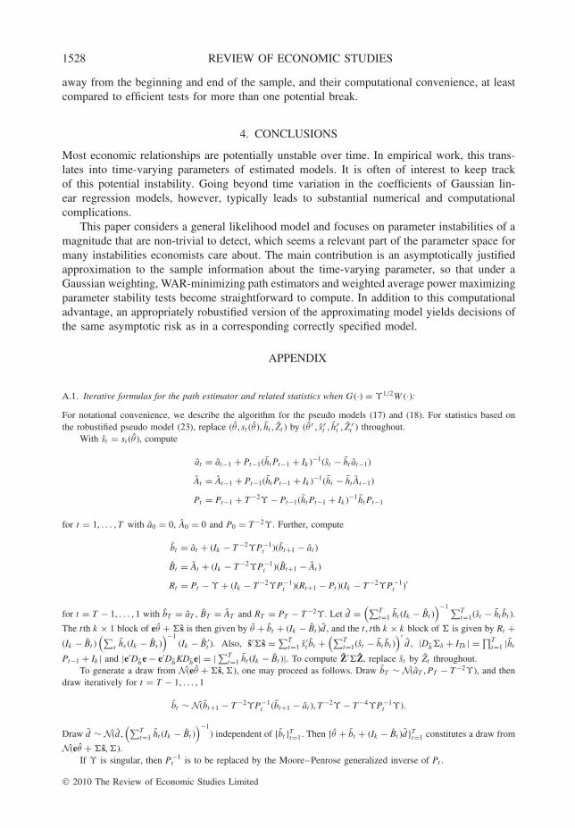
4. CONCLUSIONS
Most economic relationships are potentially unstable over time. In empirical work, this trans-lates into time-varying parameters of estimated models. It is often of interest to keep trackof this potential instability. Going beyond time variation in the coefficients of Gaussian lin-ear regression models, however, typically leads to substantial numerical and computationalcomplications.
This paper considers a general likelihood model and focuses on parameter instabilities of amagnitude that are non-trivial to detect, which seems a relevant part of the parameter space formany instabilities economists care about. The main contribution is an asymptotically justifiedapproximation to the sample information about the time-varying parameter, so that under aGaussian weighting, WAR-minimizing path estimators and weighted average power maximizingparameter stability tests become straightforward to compute. In addition to this computationaladvantage, an appropriately robustified version of the approximating model yields decisions ofthe same asymptotic risk as in a corresponding correctly specified model.
APPENDIX
A.1. Iterative formulas for the path estimator and related statistics when G(·) = ϒ1/2W (·):For notational convenience, we describe the algorithm for the pseudo models (17) and (18). For statistics based onthe robustified pseudo model (23), replace (θ , st (θ), ht , Zt ) by (θ r , s r
t , hrt , Z r
t ) throughout.With st = st (θ ), compute
at = at−1 + Pt−1(ht Pt−1 + Ik )−1(st − ht at−1)
At = At−1 + Pt−1(ht Pt−1 + Ik )−1(ht − ht At−1)
Pt = Pt−1 + T −2ϒ − Pt−1(ht Pt−1 + Ik )−1ht Pt−1
for t = 1, . . . , T with a0 = 0, A0 = 0 and P0 = T −2ϒ . Further, compute
bt = at + (Ik − T −2ϒP−1t )(bt+1 − at )
Bt = At + (Ik − T −2ϒP−1t )(Bt+1 − At )
Rt = Pt − ϒ + (Ik − T −2ϒP−1t )(Rt+1 − Pt )(Ik − T −2ϒP−1
t )′
for t = T − 1, . . . , 1 with bT = aT , BT = AT and RT = PT − T −2ϒ . Let d =(∑T
t=1 ht (Ik − Bt ))−1 ∑T
t=1(st − ht bt ).
The t th k × 1 block of eθ + �s is then given by θ + bt + (Ik − Bt )d , and the t , t th k × k block of � is given by Rt +(Ik − Bt )
(∑s hs (Ik − Bs )
)−1(Ik − B ′
t ). Also, s′�s = ∑Tt=1 s ′
t bt +(∑T
t=1(st − ht bt ))′
d , |Dh�δ + ITk | = ∏Tt=1 |ht
Pt−1 + Ik | and |e′Dh e − e′Dh KDh e| = |∑Tt=1 ht (Ik − Bt )|. To compute Z′�Z, replace st by Zt throughout.
To generate a draw from N(eθ + �s,�), one may proceed as follows. Draw bT ∼ N(aT , PT − T −2ϒ), and thendraw iteratively for t = T − 1, . . . , 1
bt ∼ N(bt+1 − T −2ϒP−1t (bt+1 − at ), T −2ϒ − T −4ϒP−1
t ϒ).
Draw d ∼ N(d ,(∑T
t=1 ht (Ik − Bt ))−1
) independent of {bt }Tt=1. Then {θ + bt + (Ik − Bt )d}T
t=1 constitutes a draw from
N(eθ + �s, �).If ϒ is singular, then P−1
t is to be replaced by the Moore–Penrose generalized inverse of Pt .
© 2010 The Review of Economic Studies Limited
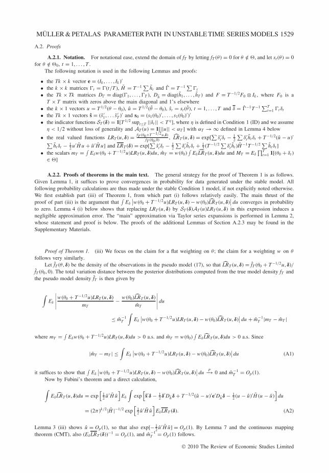
MULLER & PETALAS PARAMETER PATH IN UNSTABLE TIME SERIES MODELS 1529
A.2. Proofs
A.2.1. Notation. For notational ease, extend the domain of fT by letting fT (θ) = 0 for θ /∈ �, and let st (θ) = 0for θ /∈ �0, t = 1, . . . , T .
The following notation is used in the following Lemmas and proofs:
• the Tk × k vector e = (Ik , . . . , Ik )′
• the k × k matrices �t = �(t/T ), H = T −1 ∑ ht and � = T −1 ∑�t
• the Tk × Tk matrices D� = diag(�1, . . . ,�T ), Dh = diag(h1, . . . , hT ) and F = T −1/2F0 ⊗ Ik , where F0 is aT × T matrix with zeros above the main diagonal and 1’s elsewhere
• the k × 1 vectors u = T 1/2(θ − θ0), u = T 1/2(θ − θ0), st = st (θ ), t = 1, . . . , T and δ = �−1T −1 ∑Tt=1 �t δt
• the Tk × 1 vectors s = (s ′1, . . . s ′
T )′ and s0 = (s1(θ0)′, . . . , s1(θ0)′)′
• the indicator functions ST (δ) = 1[T 1/2 supt≤T ||δt || < T η], where η is defined in Condition 1 (ID) and we assumeη < 1/2 without loss of generality and AT (u) = 1[||u|| < αT ] with αT → ∞ defined in Lemma 4 below
• the real valued functions LRT (u, δ) = fT (θ0+T−1/2u,δ)fT (θ0,0) , LRT (u, δ) = exp[
∑s ′
t δt − 12
∑δ′
t ht δt + T −1/2(u − u)′∑ht δt − 1
2 u ′H u + u ′H u] and LRT (δ) = exp[∑
s ′t δt − 1
2
∑δ′
t ht δt + 12 (T −1/2 ∑ δ′
t ht )H −1T −1/2 ∑ ht δt ]• the scalars mT = ∫
Eδw (θ0 + T −1/2u)LRT (u, δ)du, mT = w (θ0)∫
Eδ LRT (u, δ)du and MT = Eδ
∏Tt=1 1[(θ0 + δt )
∈ �]
A.2.2. Proofs of theorems in the main text. The general strategy for the proof of Theorem 1 is as follows.Given Lemma 1, it suffices to prove convergences in probability for data generated under the stable model. Allfollowing probability calculations are thus made under the stable Condition 1 model, if not explicitly noted otherwise.We first establish part (iii) of Theorem 1, from which part (i) follows relatively easily. The main thrust of theproof of part (iii) is the argument that
∫Eδ
∣∣w (θ0 + T −1/2u)LRT (u, δ) − w (θ0)LRT (u, δ)∣∣ du converges in probability
to zero. Lemma 4 (i) below shows that replacing LRT (u, δ) by ST (δ)AT (u)LRT (u, δ) in this expression induces anegligible approximation error. The “main” approximation via Taylor series expansions is performed in Lemma 2,whose statement and proof is below. The proofs of the additional Lemmas of Section A.2.3 may be found in theSupplementary Materials.
Proof of Theorem 1. (iii) We focus on the claim for a flat weighting on θ ; the claim for a weighting w on θ
follows very similarly.Let fT (θ , δ) be the density of the observations in the pseudo model (17), so that LRT (u, δ) = fT (θ0 + T −1/2u, δ)/
fT (θ0, 0). The total variation distance between the posterior distributions computed from the true model density fT andthe pseudo model density fT is then given by
∫Eδ
∣∣∣∣∣w (θ0 + T −1/2u)LRT (u, δ)
mT− w (θ0)LRT (u, δ)
mT
∣∣∣∣∣ du
≤ m−1T
∫Eδ
∣∣w (θ0 + T −1/2u)LRT (u, δ) − w (θ0)LRT (u, δ)∣∣ du + m−1
T |mT − mT |
where mT = ∫Eδw (θ0 + T −1/2u)LRT (u, δ)du > 0 a.s. and mT = w (θ0)
∫Eδ LRT (u, δ)du > 0 a.s. Since
|mT − mT | ≤∫
Eδ
∣∣w (θ0 + T −1/2u)LRT (u, δ) − w (θ0)LRT (u, δ)∣∣ du (A1)
it suffices to show that∫
Eδ
∣∣w (θ0 + T −1/2u)LRT (u, δ) − w (θ0)LRT (u, δ)∣∣ du
p−→ 0 and m−1T = Op (1).
Now by Fubini’s theorem and a direct calculation,∫Eδ LRT (u, δ)du = exp
[12 u ′H u
]Eδ
∫exp
[s′δ − 1
2 δ′Dhδ + T −1/2(u − u)′e′Dhδ − 12 (u − u)′H (u − u)
]du
= (2π )k/2|H |−1/2 exp[
12 u ′H u
]EδLRT (δ). (A2)
Lemma 3 (iii) shows u = Op (1), so that also exp[− 12 u ′H u] = Op (1). By Lemma 7 and the continuous mapping
theorem (CMT), also (EδLRT (δ))−1 = Op (1), and m−1T = Op (1) follows.
© 2010 The Review of Economic Studies Limited
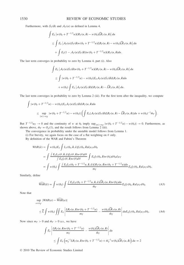
1530 REVIEW OF ECONOMIC STUDIES
Furthermore, with ST (δ) and AT (u) as defined in Lemma 4,∫Eδ
∣∣w (θ0 + T −1/2u)LRT (u, δ) − w (θ0)LRT (u, δ)∣∣ du
≤∫
Eδ
∣∣AT (u)ST (δ)w (θ0 + T −1/2u)LRT (u, δ) − w (θ0)LRT (u, δ)∣∣ du
+∫
Eδ(1 − AT (u)ST (δ))w (θ0 + T −1/2u)LRT (u, δ)du.
The last term converges in probability to zero by Lemma 4, part (i). Also∫Eδ
∣∣AT (u)ST (δ)w (θ0 + T −1/2u)LRT (u, δ) − w (θ0)LRT (u, δ)∣∣ du
≤∫
|w (θ0 + T −1/2u) − w (θ0)|EδAT (u)ST (δ)LRT (u, δ)du
+ w (θ0)∫
Eδ
∣∣AT (u)ST (δ)LRT (u, δ) − LRT (u, δ)∣∣ du.
The last term converges in probability to zero by Lemma 2 (iii). For the first term after the inequality, we compute∫|w (θ0 + T −1/2u) − w (θ0)|EδAT (u)ST (δ)LRT (u, δ)du
≤ sup||u||<αT
|w (θ0 + T −1/2u) − w (θ0)|(∫
Eδ |AT (u)ST (δ)LRT (u, δ) − LRT (u, δ)|du + w (θ0)−1mT
).
But T −1/2αT → 0 and the continuity of w at θ0 imply sup||u||<αT|w (θ0 + T −1/2u) − w (θ0)| → 0. Furthermore, as
shown above, mT = Op (1), and the result follows from Lemma 2 (iii).The convergence in probability under the unstable model follows from Lemma 1.(i) For brevity, we again focus on the case of a flat weighting on θ only.By definition of the WAR and Fubini’s Theorem
WAR(a) =∫
w (θ0)Eδ
∫LT (θ0, δ, a)fT (θ0, δ)dμT dθ0
=∫ ∫
EδLT (θ , δ, a)fT (θ , δ)w (θ)dθ∫Eδ fT (θ , δ)w (θ)dθ
∫Eδ fT (θ0, δ)w (θ0)dθ0dμT
=∫
w (θ0)∫ ∫
EδLT (θ0 + T −1/2u, δ, a)LRT (u, δ)w (θ0 + T −1/2u)du
mTEδ fT (θ0, δ)dμT dθ0.
Similarly, define
WAR(a) =∫
w (θ0)∫ ∫
EδLT (θ0 + T −1/2u, δ, a)LRT (u, δ)w (θ0)du
mTEδ fT (θ0, δ)dμT dθ0. (A3)
Note that
supa∈AT
|WAR(a) − WAR(a)|
≤ L∫
w (θ0)∫∫
Eδ
∣∣∣∣∣LRT (u, δ)w (θ0 + T −1/2u)
mT− w (θ0)LRT (u, δ)
mT
∣∣∣∣∣ duEδ fT (θ0, δ)dμT dθ0. (A4)
Now since mT > 0 and mT > 0 a.s., we have∫Eδ
∣∣∣∣∣LRT (u, δ)w (θ0 + T −1/2u)
mT− w (θ0)LRT (u, δ)
mT
∣∣∣∣∣ du
≤∫
Eδ
(m−1
T LRT (u, δ)w (θ0 + T −1/2u) + m−1T w (θ0)LRT (u, δ)
)du = 2
© 2010 The Review of Economic Studies Limited

MULLER & PETALAS PARAMETER PATH IN UNSTABLE TIME SERIES MODELS 1531
almost surely. Let MT = Eδ
∏Tt=1 1[(θ0 + δt ) ∈ �] > 0. Since � contains an open ball around θ0 and supλ∈[0,1] ||G(λ)||
is bounded almost surely, MT → 1. Note that for all T , M −1T Eδ fT (θ0, δ) is a probability density with respect to μT ,
so that the convergence in probability∫Eδ
∣∣∣∣∣LRT (u, δ)w (θ0 + T −1/2u)
mT− w (θ0)LRT (u, δ)
mT
∣∣∣∣∣ dup−→ 0
established in part (iii) of the Theorem under the unstable model with density M −1T Eδ fT (θ0, δ) implies via dominated
convergence that
MT
∫∫Eδ
∣∣∣∣∣LRT (u, δ)w (θ0 + T −1/2u)
mT− w (θ0)LRT (u, δ)
mT
∣∣∣∣∣ duM −1T Eδ fT (θ0, δ)dμT → 0
for almost all θ0. Since this is also bounded by 2, by another application of the dominated convergence theorem, wehave ∫
w (θ0)∫∫
Eδ
∣∣∣∣∣LRT (u, δ)w (θ0 + T −1/2u)
mT− w (θ0)LRT (u, δ)
mT
∣∣∣∣∣ duEδ fT (θ0, δ)dμT dθ0 → 0
so that (A4) converges to zero.Since for any a, WAR(a) − WAR(a∗) ≥ 0 by the definition of a∗ and WAR(a),
WAR(a) − WAR(a∗) =(
WAR(a) − WAR(a∗))
+(
WAR(a) − WAR(a))
+(
WAR(a∗) − WAR(a∗))
≥(
WAR(a) − WAR(a))
+(
WAR(a∗) − WAR(a∗))
→ 0.
(ii) By the Neyman Pearson Lemma, Fubini’s Theorem, and a direct calculation, the weighted average power max-imizing test of (13) under a Q∗
T weighting rejects for large values of EδLRT (0, δ − eδ), and the weighted averagepower maximizing test in the pseudo model (18) under a Q∗
T weighting rejects for large values of EδLRT (δ) (whereEδ continues to denote integration with respect to QT as defined in Condition 1). We have
|EδLRT (0, δ − eδ) − EδLRT (δ)| ≤ Eδ |ST (δ)LRT (0, δ − eδ) − LRT (δ)| + Eδ(1 − ST (δ))LRT (0, δ − eδ)p−→ 0
by applying Lemmas 4 (ii) and 2 (iv). Furthermore, the asymptotic distribution of EδLRT (δ) under the null hypothesisis absolutely continuous by Lemma 7, so that the result follows from the second claim in Lemma 1 by the samearguments as employed in Andrews and Ploberger (1994) in the proof of their Theorem 2.
Proof of Theorem 2. (iii) In matrix form, the pseudo model (17) is s + Dh eθ |(Dh , δ, θ) ∼ N(Dh (δ + eθ), Dh ), sothat conditionally on Dh and θ only,(
s + Dh eθδ
)|(Dh , θ) ∼ N
((Dh eθ
0
),
(Dh + Dh�δDh Dh�δ
�δDh �δ
)).
Using the identity
(ITk + Dh�δ)−1 = ITk − (ITk + Dh�δ)−1Dh�δ (A5)
we find with K = �δDh (Dh + Dh�δDh )−1 = �δ − �δDh (Dh + Dh�δDh )−1Dh�δ that
δ|(s + Dh eθ , Dh , θ) ∼ N(K (s + Dh e(θ − θ)), K ).
Furthermore, with a flat prior, the posterior for θ is proportional to the likelihood, so that (s + Dh eθ)|(Dh , θ) ∼N(Dh eθ , Dh + Dh�δDh ) implies θ |(s + Dh eθ , Dh ) ∼ N((e′(D−1
h+ �δ)−1e)−1e′(D−1
h+ �δ)−1D−1
hs + θ , (e′(D−1
h+
�δ)−1e)−1). Thus(δ
θ
)|(s + Dh eθ , Dh ) ∼ N
((K (s − Dh e(e′(D−1
h+ �δ)−1e)−1e′(D−1
h+ �δ)−1D−1
hs)
(e′(D−1h
+ �δ)−1e)−1e′(D−1h
+ �δ)−1D−1h
s + θ
), Vδθ
)
where Vδθ =(
K + KDh e(e′(D−1h
+ �δ)−1e)−1e′Dh K −KDh e(e′(D−1h
+ �δ)−1e)−1
−(e′(D−1h
+ �δ)−1e)−1e′Dh K (e′(D−1h
+ �δ)−1e)−1
)© 2010 The Review of Economic Studies Limited

1532 REVIEW OF ECONOMIC STUDIES
and employing once more (A5), we conclude δ + eθ |(s + Dh eθ , Dh ) ∼ N(eθ + �s, �).(i) Immediate from Theorem 1 (i) and the proof of part (i).(ii) Note that with v = T −1/2(u − u), by Fubini’s Theorem and (A2),
(2π )k/2|e′Dh e|−1/2EδLRT (δ) =∫
Eδ exp[s′δ − 1
2 δ′Dhδ + v ′e′Dhδ − 12 v ′e′Dh ev
]dv
= |Dh�δ + ITk |−1/2∫
exp[ 1
2 (s + Dh ev )′K (s + Dh ev ) − 12 v ′e′Dh ev
]dv
= (2π )k/2|Dh�δ + ITk |−1/2|e′Dh e − e′Dh KDh e|−1/2 exp[ 1
2 s′�s]. (A6)
Now let R(δ) = exp[− 12 δ′Dhδ + 1
2 δ′Dh e(e′Dh e)−1e′Dhδ], so that
EδLRT (δ)
EδR(δ)= exp
[12 s′�s
].
By Lemma 2 (ii), EδR(δ) − Eδ exp[− 12 δ′D�(δ − eδ)]
p−→ 0. By the CMT, exp[− 12 δ′D�(δ − eδ)] ⇒ exp[− 1
2
∫ 10 G∗(s)′
�(s)G∗(s)ds], and since R(δ) < 1 a.s., also EδR(δ) → EG exp[− 12
∫ 10 G∗(s)′�(s)G∗(s)ds]. The result now follows
from Lemma 7.
Proof of Theorem 3. We write �t for �T ,t to enhance readability, and let D� = diag(�1, . . . , �T ).For the first claim, note that if {ht }T
t=1 satisfies (16), so does �′t ht and �′
t ht �t . Also, by summation by parts with�0 = �1
T −1/2t∑
j=1
�′j sj (θ ) = �′
t T−1/2
t∑j=1
sj (θ ) −t∑
j=1
(�′j − �′
j−1)(T −1/2j−1∑l=1
sl (θ ))
so that T −1/2 ∑[·T ]j=1 sj ⇒ SL(·) implies T −1/2 ∑[·T ]
j=1 �′j sj ⇒ SL(·). The result thus follows from Theorem 2 (ii).
For the second claim, proceed as in the proof of part (i) of Theorem 1, but with WAR(a) in (A3) substituted by
WAR�(a) =∫
w (θ0)∫ ∫
Eδw (θ0)LRT (u, D�δ)L(θ0 + T −1/2u, D�δ, a)du
m�,TEδ fT (θ0, δ)dμT dθ0
where m�,T = ∫Eδw (θ0)LRT (u, D�δ)du. We have
|WAR�(a) −∫
w (θ0)∫ ∫
Eδw (θ0)LRT (u, D�δ)L(θ0 + T −1/2u, δ, a)du
m�,TEδ fT (θ0, δ)dμT dθ0|
≤∫
w (θ0)
⎛⎝ supθ∈�,δ∈RTk ,a∈AT
|LT (θ , D�δ, a) − LT (θ , δ, a)|⎞⎠Eδ fT (θ0, δ)dμT dθ0 → 0
where the convergence follows from supθ∈�,δ∈RTk ,a∈AT
|LT (θ , D�δ, a) − LT (θ , δ, a)| p−→ 0 in the stable model,
Lemma 1 and the dominated convergence theorem as supθ∈�,δ∈RTk ,a∈AT
|LT (θ , D�δ, a) − LT (θ , δ, a)| ≤ 2L. It thus
suffices to proceed as in the proof of Theorem 1 with LRT (u, δ) replaced by LRT (u, D�δ), and the result follows fromTheorem 2 (i), as in the proof of the first claim.
Proof of Theorem 4. For the claim regarding the analogous statement of Theorem 1 (iii), proceed up to equation(A1) as in the proof of Theorem 1 (iii) with Eδ now denoting integration with respect to the mixture. With Eδ(i )
denoting integration with respect to the measure of {T −1/2Gi (t/T )}, it then suffices to show that∫
Eδ(i )|w (θ0 +T −1/2u)LRT (u, δ(i )) − w (θ0)LRT (u, δ(i ))|du
p−→ 0 for i = 1, . . . , nG and m∗−1T = (
∑i pi m(i ),T )−1 = Op (1), where m(i ),T
= w (θ0)∫
Eδ(i )LRT (u, δ(i ))du. From the same reasoning as in the proof of Theorem 1 (iii), m−1(i ),T = Op (1), so that
also m∗−1T = Op (1). The result now follows by proceeding as in the remainder of the proof of Theorem 1 (iii) and by
invoking Lemmas 4 (i) and 2 (iii) for each of the nG components in the measure of δ.The conditionally normal distribution N(eθ + �i s,�i ) follows as in the proof of Theorem 2. For the mixing
probabilities, note that the Bayes factor between pseudo models i and j is given by m(i ),T /m(j ),T . Using (A2) and(A6), we find
m(i ),T
m(j ),T= |Dh�δ(i ) + ITk |−1/2|e′Dh e − e′Dh Ki Dh e|−1/2 exp[ 1
2 s′�i s]
|Dh�δ(j ) + ITk |−1/2|e′Dh e − e′Dh Kj Dh e|−1/2 exp[ 12 s′�j s]
so that the posterior odds of model i and model j in the pseudo model are as stated.
© 2010 The Review of Economic Studies Limited
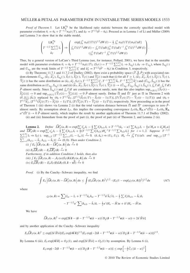
MULLER & PETALAS PARAMETER PATH IN UNSTABLE TIME SERIES MODELS 1533
Proof of Theorem 5. Let LRπ0T be the likelihood ratio statistic between the correctly specified model with
parameter evolution θt = θ0 + T −1/2π0(t/T ), and uT = T 1/2(θ − θ0). Proceed as in Lemma 1 of Li and Muller (2009)and Lemma 3 to show that in the stable model,⎛⎜⎝ LR
π0T
T −1/2 ∑[·T ]t=1 st
uT
⎞⎟⎠ ⇒
⎛⎜⎜⎝exp[
∫ 10 π0(l )′�(l )1/2dW (l ) − 1
2
∫ 10 π0(l )′�(l )π0(l )dl ]∫ ·
0 �(l )1/2dW (l ) − ∫ ·0 �(l )dl (
∫ 10 �(l )dl )−1
∫ 10 �(l )1/2dW (l )
(∫ 1
0 �(l )dl )−1∫ 1
0 �(l )1/2dW (l )
⎞⎟⎟⎠ .
Thus, by a general version of LeCam’s Third Lemma (see, for instance, Pollard, 2001), we have that in the unstablemodel with parameter evolution θt = θ0 + T −1/2π0(t/T ), (ST (·) = T −1/2 ∑[·T ]
t=1 st ⇒ Sπ0 (·), uT ⇒ Uπ0 ), where Sπ0 (·)and Uπ0 are the weak limits of T −1/2 ∑[·T ]
t=1 s rt and ur
T = T 1/2(θ r − θ0) in Condition 3, respectively.(i) By Theorems 11.7.1 and 11.7.2 of Dudley (2002), there exist a probability space (F, F, P ) with associated ran-
dom elements Uπ0 , (uT ,˜urT ), Sπ0 (·), ST (·), S r
T (·), ϒT (·) and ϒ rT (·) such that (i) for all T ≥ 1, (uT ,˜ur
T , ST (·), S rT (·), ϒT (·),
ϒ rT (·)) has the same distribution as (uT , ur
T , ST (·), T −1/2 ∑[·T ]t=1 s r
t , T −1 ∑[·T ]t=1 ht , T −1 ∑[·T ]
t=1 hrt ) and (Uπ0 , Sπ0 (·)) has the
same distribution as (Uπ0 , Sπ0 (·)); and (ii) (uT ,˜urT , ST (·), S r
T (·), ϒT (·), ϒ rT (·)) → (Uπ0 , Uπ0 , Sπ0 (·), Sπ0 (·), ∫ ·
0 �dl ,∫ ·
0 �dl )P -almost surely. Since Sπ0 (·) and
∫ ·0 �dl are continuous almost surely, note that this also implies supλ∈[0,1] ||ST (λ) −
S rT (λ)|| → 0 and supλ∈[0,1] ||ϒT (λ) − ϒ r
T (λ)|| → 0 P -almost surely. Define � and �r just as � in Theorem 2 with(θ , {st }, {ht }) replaced by (θ0 + T 1/2˜uT , {T 1/2(ST (t/T ) − ST ((t − 1)/T )}, {T (ϒT (t/T ) − ϒT ((t − 1)/T )}) and (θ0 +T 1/2˜ur
T , {T 1/2(S rT (t/T ) − S r
T ((t − 1)/T )}, {T (ϒ rT (t/T ) − ϒ r
T ((t − 1)/T )}), respectively. Now proceeding as in the proofof Theorem 1 (iii) shows via Lemma 2 (i) that the total variation distance between � and �r converges to zero P -almost surely. By assumption about LT , this implies the corresponding convergence LT (θ0, π0, a∗(�)) − LT (θ0, π0,a∗(�r )) → 0 P-almost surely, which implies the result by another application of Theorem 11.7.1 of Dudley (2002).
(ii) and (iii) Immediate from the proof of part (i), the proof of part (ii) of Theorem 2, and Lemma 2 (ii).
Lemma 2. Define LRaT (u, δ) = exp[
∑s ′
at δt − 12
∑δ′
t ha1t δt + T −1/2(ua − u)′∑
ha2t δt − 12 u ′Ha u + u ′
a Ha u]and LR
aT (δ) = exp[
∑s ′
at δt − 12
∑δ′
t ha1t δt + 12 (T −1/2 ∑ δ′
t ha2t )H −1a T −1/2 ∑ ha2t δt ] for i = 1, 2. Suppose T −1/2∑[·T ]
t=1 st ⇒ SL(·), supt≤T ||T −1/2 ∑ts=1(ss − sas )|| p−→ 0, (u, ua ) ⇒ (UL, UL), Ha
p−→ ∫ 10 �(λ)dλ and supt≤T ||T −1∑t
s=1(ha1s − hs , ha2s − hs )|| p−→ (0, 0). Then under Condition 2,
(i)∫
Eδ
∣∣∣LRT (u, δ) − LRaT (u, δ)
∣∣∣ dup−→ 0
(ii) EδLRT (δ) − EδLRaT (δ)
p−→ 0Furthermore, if in addition Condition 1 holds, then also(iii)
∫Eδ
∣∣LRT (u, δ) − AT (u)ST (δ)LRT (u, δ)∣∣ du
p−→ 0
(iv) EδLRT (δ) − EδST (δ)LRT (0, δ − eδ)p−→ 0
Proof. (i) By the Cauchy–Schwarz inequality, we find∫Eδ
∣∣∣LRT (u, δ) − LRaT (u, δ)
∣∣∣ du ≤∫
(Eδ LRT (u, δ)2)1/2 · (Eδ(1 − exp[ςT (u, δ)])2)1/2du (A7)
where
ςT (u, δ) =∑
(sat − st + T −1/2ua hat − T −1/2u ′ht )′δt − 1
2
∑δ′
t (ha1t − ht )δt
− T −1/2u ′ ∑(ha2t − ht )δt − 12 u ′(Ha − H )u + u ′(Ha − H )u.
We have
LRT (u, δ)2 = exp[2s′δ − (δ − T −1/2e(u − u))′Dh (δ − T −1/2e(u − u)) + 2u ′H u]
and by another application of the Cauchy–Schwarz inequality
Eδ LRT (u, δ)2 ≤ exp[2u ′H u](Eδ exp[4s′δ])1/2(Eδ exp[−2(δ − T −1/2e(u − u))′Dh (δ − T −1/2e(u − u))])1/2.
By Lemma 6 (iii), Eδ exp[4s′δ] = Op (1), and exp[2u ′H u] = Op (1) by assumption. By Lemma 6 (i),
Eδ exp[−2(δ − T −1/2e(u − u))′Dh (δ − T −1/2e(u − u))] ≤ exp[− 1
2 CT ||u − u||2]
© 2010 The Review of Economic Studies Limited
1534 REVIEW OF ECONOMIC STUDIES
where CT = Op (1) and C −1T = Op (1) and does not depend on u. Therefore,
Eδ LRT (u, δ)2 ≤ Op (1)(2π )−k/2C k/2T exp
[− 1
2 CT ||u − u||2]
(A8)
so that with �(u) the c.d.f. of u ∼ N(u, C −1T Ik ), from (A7) and Jensen’s inequality(∫
Eδ
∣∣∣LRT (u, δ) − LRaT (u, δ)
∣∣∣ du
)2
≤ K1T
∫Eδ(1 − exp[ςT (u, δ)])2d�(u)
where K1T = Op (1), so that is suffices to show that∫
Eδ exp[ςT (u, δ)]d�(u) is bounded below by a random variablethat converges to one in probability, and
∫Eδ exp[2ςT (u, δ)]d�(u) is bounded above by a random variable that
converges to one in probability. By Lemma 6 (ii), there exist random variables κTp−→ 1, κT
p−→ 1, �Tp−→ 0 and
�Tp−→ 0 such that∫
Eδ exp[ςT (u, δ)]d�(u) ≥ κT
∫exp
[�T ||u||2 − 1
2 u ′(Ha − H )u + u ′(Ha − H )u]
d�(u)]d�(u)∫Eδ exp[2ςT (u, δ)]d�(u) ≤ κT
∫exp
[�T ||u||2 − 1
2 u ′(Ha − H )u + u ′(Ha − H )u]
d�(u)]d�(u)
and the result follows.(ii) By a direct calculation,
(2π )−k/2|H |−1/2 exp[
12 u ′H u
]|EδLRT (δ) − EδLR
aT (δ)|
=∣∣∣∣Eδ
∫LRT (u, δ)du − Eδ
∣∣∣∣Ha |1/2|H |−1/2 exp[− 1
2 u ′(Ha − H )u] ∫
LRaT (u, δ)du|
≤∫
Eδ
∣∣∣LRT (u, δ) − LRaT (u, δ)
∣∣∣ du + |1 − |Ha |1/2|H |−1/2 exp[− 1
2 u ′(Ha − H )u]|Eδ
∫LR
aT (u, δ)du
and the result follows from part (i) and |Ha |1/2|H |−1/2 exp[− 12 u ′(Ha − H )u]
p−→ 1.(iii) Let UT be the indicator of the event that ||u|| ≤ αT . By Lemma 3 (iii), u = Op (1), so that EUT → 1.
Note that if UT ψTp−→ 0 for some sequence of random variables ψT , then also ψT
p−→ 0. Let T be large enoughsuch that �T = {θ : ||θ − θ0|| < 2T −1/2αT + T η−1/2 + T η−1/2(supλ∈[0,1] ||�(λ)||)/(infλ∈[0,1] ||�(λ)||)} ⊂ �0, so thatθ0 + AT (u)ST (δ)UT (T −1/2(u − u) + δt − δ) ∈ �0 almost surely for all t ≤ T .
Let gv : [0, 1] → R with gv (λ) = lt (θ0 + λv ) − lt (θ0). Note that for θ0 + v ∈ �T , gv is twice continuously differ-entiable with g ′
v (λ) = v ′st (θ0 + λv ) and g ′′v (λ) = −v ′ht (θ0 + λv )v , so that by a first order Taylor expansion in the inte-
gral remainder form, lt (θ0 + v ) − lt (θ0) = gv (1) − gv (0) = g ′v (0) + ∫ 1
0 λg ′′v (1 − λ)dλ = v ′st (θ0) − 1
2 v ′(2∫ 1
0 λht (θ0 +(1 − λ)v )dλ)v , and similarly, st (θ0 + v ) = st (θ0) − (
∫ 10 ht (θ0 + λv )dλ)v . Thus, for ||u|| < αT , T 1/2 supt≤T ||δt || < T η
and ||u|| < αT
lt (θ0 + T −1/2u + δt ) − lt (θ0 + T −1/2u) = st (θ0 + T −1/2u)′δt − 12 δ
′t h1,t (u, δ)δt
lt (θ0 + T −1/2u) − lt (θ0) = T −1/2u ′st (θ0) − 12 u ′h2,t (u)u
st (θ0 + T −1/2u) = st (θ0 + T −1/2u) − h3,t (u, u)T −1/2(u − u)
st (θ0) = st (θ0 + T −1/2u) + h4,t (u)T −1/2u (A9)
almost surely, where h1,t (u, δ) = 2∫ 1
0 λht (θ0 + T −1/2u + (1 − λ)δt )dλ, h2,t (u) = 2∫ 1
0 λht (θ0 + (1 − λ)T −1/2u)dλ,h3,t (u, u) = ∫ 1
0 ht (θ0 + λT −1/2(u − u))dλ and h4,t (u) = ∫ 10 ht (θ0 + λT −1/2u)dλ, t = 1, . . . , T . Define {h1,t (u, δ)}T
t=1 ={ht (θ0)}T
t=1 when ||u|| ≥ αT or T 1/2 supt≤T ||δt || > T η, define {h2,t (u)}Tt=1 = {ht }T
t=1 when ||u|| ≥ αT , define{h3,t (u, u)}T
t=1 = {ht }Tt=1 when ||u|| ≥ αT or ||u|| ≥ αT , and define {h4,t (u)}T
t=1 = {ht }Tt=1 when ||u|| > αT . Further,
let H4(u) = T −1 ∑ h4,t (u) and H2(u) = T −1 ∑ h2,t (u). For notational convenience, we drop the dependence of h1,t ,h2,t , H3 and H4 on u, u and δ. With these definitions, we have
AT (u)ST (δ)UT
∣∣∣LRT (u, δ) − exp[∑
s ′t δt + T −1/2(u − u)′
∑h3,t δt − 1
2
∑δ′
t h1,t δt + u ′H4u − 12 u ′H2u
]∣∣∣ = 0
almost surely, uniformly in u ∈ Rk and δ ∈ RTk .
© 2010 The Review of Economic Studies Limited

MULLER & PETALAS PARAMETER PATH IN UNSTABLE TIME SERIES MODELS 1535
Let
ςT (u, δ) = (u − u)′T −1/2∑
(h3,t − ht )δt − 12
∑δ′
t (h1,t − ht )δt − 12 u ′(H2 − H )u + u ′(H4 − H )u.
Now supu∈Rk ,δ∈RTk AT (u)ST (δ)UT |LRT (u, δ) − LR(u, δ) exp ςT (u, δ)| = 0 a.s., and by the Cauchy–Schwarz inequalityand UT ≤ 1 a.s.
UT
∫Eδ
∣∣LRT (u, δ) − AT (u)ST (δ)LRT (u, δ)∣∣ du
≤∫
[(Eδ LRT (u, δ)2)(Eδ(1 − AT (u)ST (δ) exp ςT (u, δ))2)]1/2du.
Proceeding as in the proof of part (i), it suffices to show that∫
Eδ(1 − AT (u)ST (δ) exp ςT )2d�(u)p−→ 0. We first
compute the expectation with respect to δ. This is complicated by the fact that h1,t depends on δ. To circumventthis problem, we bound ςT (u, δ) by ς
T(u, δ) ≤ ςT (u, δ) ≤ ςT (u, δ), where ς
T(u, δ) and ςT (u, δ) are defined just as
ςT (u, δ), but with h1,t replaced by a term that does not depend on δ (or u).Specifically, for each t ≤ T , define dt = 2 sup||v ||<αT +Tη
∥∥ht (θ0 + T −1/2v ) − ht (θ0)∥∥, so that for any υ ∈ Rk
with ||υ|| = 1,
|υ ′(ht (θ0) − h1,t )υ| ≤ ||ht (θ0) − h1,t || ≤ dt
since for ||u|| < αT and T 1/2 supt≤T ||δt || < T η, ||ht (θ0) − h1,t || = ||2 ∫ 10 λ(ht (θ0 + T −1/2u + (1 − λ)δt ) − ht (θ0))dλ||
and h1,t (u, δ) = ht (θ0) otherwise. Thus, for all δ ∈ RTk ,∑δ′
t (ht (θ0) − dt Ik ) δt ≤∑
δ′t h1,t δt ≤
∑δ′
t (ht (θ0) + dt Ik ) δt .
Now let
ςT (u, δ) = ςT (u, δ) + 12
∑δ′
t (h1,t − ht (θ0) + dt Ik )δt
ςT
(u, δ) = ςT (u, δ) + 12
∑δ′
t (h1,t − ht (θ0) − dt Ik )δt
so that ςT
(u, δ) ≤ ςT (u, δ) ≤ ςT (u, δ). We obtain
0 ≤ Eδ(1 − AT (u)ST (δ) exp ςT (u, δ))2
≤ 1 − 2EδAT (u)ST (δ) exp ςT
(u, δ) + EδAT (u)ST (δ) exp 2ςT (u, δ)
≤ 1 − 2Eδ exp ςT
(u, δ) + Eδ exp 2ςT (u, δ) + 2Eδ(1 − AT (u)ST (δ)) exp ςT
(u, δ)
so it suffices to show that∫
Eδ exp ςT
(u, δ)d�(u) is bounded below by random variable that converges to one inprobability, that
∫Eδ exp 2ςT (u, δ)d�(u) is bounded above by a random variable that converges to one in probability,
and∫
Eδ(1 − ST (δ)AT (u)) exp ςT
(u, δ)d�(u)p−→ 0.
With Dh3 = diag(h3,1, . . . , h3,T ), Dh = diag(h1(θ0), . . . , hT (θ0)) and Dd = diag(d1Ik , . . . , dT Ik ) we have
Eδ exp ςT
(u, δ) = exp[− 1
2 u ′(H2 − H )u + u ′(H4 − H )u]
·Eδ exp[(u − u)′T −1/2e′(Dh3 − Dh )δ − 1
2 δ′(Dh − Dh + Dd )δ]
and
Eδ exp 2ςT (u, δ) = exp[−u ′(H2 − H )u + 2u ′(H4 − H )u]
·Eδ exp[2(u − u)′T −1/2e′(Dh3 − Dh )δ − δ′(Dh − Dh − Dd )δ].
Since
supu∈Rk ,t≤T
T −1
∥∥∥∥∥t∑
s=1
(h3,s (u, u) − hs )
∥∥∥∥∥ ≤ supt≤T ,||u||≤αT ,||u||<αT
T −1
∥∥∥∥∥t∑
s=1
h3,s (u, u) − hs
∥∥∥∥∥ p−→ 0
supt≤T
T −1
∥∥∥∥∥t∑
s=1
(hs (θ0) + dt Ik − hs )
∥∥∥∥∥ ≤ supt≤T
∥∥∥∥∥T −1t∑
s=1
(hs (θ0) − hs )
∥∥∥∥∥ + T −1T∑
t=1
dtp−→ 0
© 2010 The Review of Economic Studies Limited

1536 REVIEW OF ECONOMIC STUDIES
by (16), Lemma 3 (ii) and Condition 1 (LLLN), and similarly, supt≤T ||T −1 ∑ts=1(hs (θ0) − dt Ik − �s )|| p−→ 0, Lemma 6
(ii) is applicable, and we obtain
Eδ exp ςT
(u, δ) ≥ exp[− 1
2 u ′(H2 − H )u + u ′(H4 − H )u]κT exp[�T ||u − u||2]
Eδ exp 2ςT (u, δ) ≤ exp[−u ′(H2 − H )u + 2u ′(H4 − H )u]κT exp[�T ||u − u||2]
uniformly in u, where κT , κT , �T and �T do not depend on u and κTp−→ 1, κT
p−→ 1, �Tp−→ 0 and �T
p−→ 0.Also
supu∈Rk
||H2(u) − H || ≤ sup||u||<αT
T −1||∑
h2,t (u) − �t || p−→ 0
by (16) and Lemma 3 (ii), and similarly, H4 − Hp−→ 0. Thus,
∫Eδ exp ς
T(u, δ)d�(u) ≥ ∫
κ∗T exp[�∗
T ||u − u||2]
d�(u)p−→ 1 and
∫Eδ exp 2ςT (u, δ)d�(u) ≤ ∫
κ∗T exp[�
∗T ||u − u||2]d�(u)
p−→ 1 for suitably defined κ∗T
p−→ 1, κ∗T
p−→1, �∗
Tp−→ 0 and �
∗T
p−→ 0. We are left to show that∫
Eδ(1 − ST (δ)AT (u)) exp ςT
d�(u)p−→ 0. By the Cauchy–Schwarz
inequality[∫Eδ(1 − ST (δ)AT (u)) exp ς
T(u, δ)d�(u)
]2
≤[∫
Eδ(1 − ST (δ)AT (u))2d�(u)
] [∫Eδ exp 2ς
T(u, δ)d�(u)
].
From the same reasoning as above,∫
Eδ exp 2ςT
(u, δ)d�(u) = Op (1), and∫Eδ(1 − ST (δ)AT (u))d�(u) ≤
∫Eδ(1 − ST (δ))d�(u) +
∫Eδ(1 − AT (u))d�(u).
But∫
Eδ(1 − ST (δ))d�(u) = Eδ(1 − ST (δ)) = Eδ1[T 1/2 supt≤T ||δt || ≥ T η] → 0, and∫
Eδ(1 − AT (u))d�(u) ≤∫1[||u|| ≥ αT ]d�(u)
p−→ 0 since ||u|| = Op (1), C −1/2T = Op (1) and αT → ∞.
(iv) Similar to the proof of part (iii) and omitted for brevity.
A.2.3. Additional lemmas.
Lemma 3. Under Condition 1:(i) T −1/2 ∑[·T ]
t=1 st (θ0) ⇒ ∫ ·0 �1/2(l )dW (l ), where W is a k × 1 standard Wiener process
(ii) supt≤T ,{vt }Tt=1∈BT
T ,{vt }Tt=1∈BTT
T −1‖∑ts=1(2
∫ 10 λhs (θ0 + vs + λvs )dλ − �s )‖ p−→ 0 and sup
t≤T ,{vt }Tt=1∈BTT ,{vt }Tt=1∈BT
T
T −1||∑ts=1(
∫ 10 hs (θ0 + λ(vs − vs ))dλ − �s )|| p−→ 0, where BT = {θ : ||θ − θ0|| < bT } with bT → 0, and BT
T = BT
× · · · × BT
(iii) u = T 1/2(θ − θ0) = Op (1)(iv) T −1/2 ∑[·T ]
t=1 st (θ ) ⇒ ∫ ·0 �(l )1/2dW (l ) − ∫ ·
0 �(l )dl (∫ 1
0 �(l )dl )−1∫ 1
0 �(l )1/2dW (l )
(v) supλ∈[0,1] ||T −1 ∑[λT ]t=1 st (θ )st (θ )′ − ∫ λ
0 �(l )dl || p−→ 0 and T −1 ∑ st (θ0)st (θ0)′ = Op (1)
(vi) supλ∈[0,1] ||T −1 ∑[λT ]t=1 ht (θ ) − ∫ λ
0 �(l )dl || p−→ 0.
Lemma 4. Under Conditions 1 and 2, there exists a sequence of real numbers αT with αT → ∞ and T −1/2αT →0 such that
(i)∫
w (θ0 + T −1/2u)Eδ (1 − AT (u)ST (δ))LRT (u, δ)dup−→ 0
(ii) Eδ(1 − ST (δ))LRT (0, δ − eδ)p−→ 0.
Lemma 5. Let ��(u) be a Tk × Tk matrix consisting of k × k blocks �i ,j (u), i , j = 1, . . . , T , possibly dependenton u and define cU
T = supi ,j≤T ,u∈Rk ||�i ,j (u)||. Under Condition 2, there exists a constant cG independent of u and Tsuch that
(i) |tr((F−1�δF ′−1)��(u))| ≤ cUT cG
(ii) |tr((F−1�δF ′−1)��(u)(F−1�δF ′−1)��(u))| ≤ (cUT )2c2
G .
© 2010 The Review of Economic Studies Limited

MULLER & PETALAS PARAMETER PATH IN UNSTABLE TIME SERIES MODELS 1537
Lemma 6. Under Condition 1:(i) There exists a sequence of random variables CT = Op (1) satisfying C −1
T = Op (1) such that
supv∈Rk ,T
(Eδ exp[−2(δ − T −1/2ev )′Dh (δ − T −1/2ev )] − exp[− 12 CT ||v ||2]) ≤ 0.
(ii) Suppose the k × 1 vectors ξt satisfy supt≤T ||T −1/2 ∑ts=1 ξs || p−→ 0, the k × k matrix functions ζt : Rk → Rk×k
satisfy supt≤T ,u∈Rk ||T −1 ∑ts=1 ζs (u)|| p−→ 0, the k × k matrices �it satisfy supt≤T ||T −1 ∑t
s=1 �is || p−→ 0, i = 1, 2, 3.Then, with ξ = (ξ ′
1, . . . , ξ ′T )′, Dζ (u) = diag(ζ1(u), . . . , ζT (u)), �i = (�′
i1, . . . , �′iT )′, i = 1, 2 and D� = diag(�31, . . . ,�3T )
κT exp[�T ||v ||2] ≤ Eδ exp[ξ ′δ + T −1/2v ′e′Dζ (u)δ − 1
2 δ′(T −1�1�′2 + D�)δ
] ≤ κT exp[�T ||v ||2]
uniformly in v and T , where the scalar random variables κT , �T , κT and �T do not depend on u or v and κTp−→ 1,
κTp−→ 1, �T
p−→ 0 and �Tp−→ 0.
(iii) If T −1/2 ∑[·T ]t=1 st ⇒ SL(·), then Eδ exp[4s′δ] = Op (1).
(iv) If JT ∈ D is a nonstochastic sequence converging to J ∈ D, where D is the set of cadlag functions on the unitinterval, then
supT
Eδ exp[T 1/2JT (1)′(δT − δ) − T 1/2∑
JT ((t − 1)/T )′(δt − δt−1)] < ∞
with δ0 = 0.
Lemma 7. Under Conditions 1 and 2,
EδLRT (δ) ⇒ EG exp
[∫ 1
0G∗(s)�(s)1/2dW (s) − 1
2
∫ 10 G∗(s)′�(s)G∗(s)ds
]
where G∗(s) = G(s) − (∫ 1
0 �(λ)dλ)−1∫ 1
0 �(λ)G(λ)dλ.
Acknowledgements. We benefitted from thoughtful and constructive comments and suggestions by the editor,Enrique Sentana, and two anonymous referees. We would also like to thank Mark Watson, as well as participantsat the NBER Summer Institute, the Workshop for Nonlinear and Nonstationary Models at the California Institute ofTechnology, the Unit Root and Cointegration Testing Conference in Faro, the Econometric Society World Congressin London, and workshops at the University of Lausanne, New York University, Rutgers University, University ofTexas at Austin, FRB of Atlanta, and Iowa State University for useful discussions, and Edouard Schaal for excellentresearch assistance. Muller gratefully acknowledges financial support from the NSF through grant SES-0518036.
REFERENCES
ANDERSON, T. W. (1955), “The Integral of a Symmetric Convex Set and some Probability Integrals”, Proceedingsof the American Mathematical Society, 6, 170–176.
ANDREWS, D. W. K. and PLOBERGER, W. (1994), “Optimal Tests When a Nuisance Parameter Is Present Onlyunder the Alternative”, Econometrica, 62, 1383–1414.
BAI, J. (1997), “Estimation of a Change Point in Multiple Regressions”, Review of Economics and Statistics, 79,551–563.
BAI, J. and PERRON, P. (1998), “Estimating and Testing Linear Models with Multiple Structural Changes”, Econo-metrica, 66, 47–78.
BERNANKE, B. S. and MIHOV, I. (1998), “Measuring Monetary Policy”, The Quarterly Journal of Economics, 113,869–902.
BILLINGSLEY, P. (1968), “Convergence of Probability Measure” (New York: Wiley).BOIVIN, J. (2003), “Has U.S. Monetary Policy Changed? Evidence from Drifting Coefficients and Real Time Data”
(Working Paper, Columbia University).BROWN, L. D. and LOW, M. G. (1996), “Asymptotic Equivalence of Nonparametric Regression and White Noise”,
Annals of Statistics, 24, 2384–2398.CAI, Z. (2007), “Trending Time-Varying Coefficient Time Series Models with Serially Correlated Errors”, Journal of
Econometrics, 136, 163–188.
© 2010 The Review of Economic Studies Limited

1538 REVIEW OF ECONOMIC STUDIES
CHIB, S. (1998), “Estimation and Comparison of Multiple Change-Point Models”, Journal of Econometrics, 75,221–241.
COGLEY, T. and SARGENT, T. J. (2005), “Drifts and Volatilities: Monetary Policies and Outcomes in the PostWWII US”, Review of Economic Dynamics, 8, 262–302.
DUDLEY, R. M. (2002), Real Analysis and Probability (Cambridge, UK: Cambridge University Press).DUFOUR, J.-M. and GHYSELS, E. (1996), “Recent Developments in the Econometrics of Structural Change:
Overview”, Journal of Econometrics, 70, 1–8.DURBIN, J. and KOOPMAN, S. J. (1997), “Monte Carlo Maximum Likelihood Estimation for Non-Gaussian State
Space Models”, Biometrika, 84, 669–684.DURBIN, J. and KOOPMAN, S. J. (2001), “Time Series Analysis by State Space Methods” (Oxford: Oxford Uni-
versity Press).ELLIOTT, G. and MULLER, U. K. (2006), “Efficient Tests for General Persistent Time Variation in Regression
Coefficients”, Review of Economic Studies, 73, 907–940.ELLIOTT, G. and MULLER, U. K. (2007), “Confidence Sets for the Date of a Single Break in Linear Time Series
Regressions”, Journal of Econometrics, 141, 1196–1218.FERNANDEZ-VILLAVERDE, J. and RUBIO-RAMIREZ, J. (2007), “How Structural Are Structural Parameters?”,
Macroeconomics Annual, 22, 83–137.GHYSELS, E. (1998), “On Stable Factor Structures in the Pricing of Risk: Do Time-Varying Betas Help or Hurt?”,
Journal of Finance, 53, 549–573.GOURIEROUX, C., MONFORT, A. and TROGNON, A. (1984), “Pseudo Maximum Likelihood Methods: Theory”,
Econometrica, 52, 681–700.HALL, P. and HEYDE, C. C. (1980), Martingale Limit Theory and its Applications (New York: Academic Press).HAMILTON, J. D. (1989), “A New Approach to the Economic Analysis of Nonstationary Time Series and the Business
Cycle”, Econometrica, 57, 357–384.HANSEN, B. E. (1996), “Inference When a Nuisance Parameter Is Not Identified Under the Null Hypothesis”, Econo-
metrica, 64, 413–430.HARVEY, A. C. (1989), “Forecasting, Structural Time Series Models and the Kalman Filter” (Cambridge University
Press).HARVEY, A. C., RUIZ, E. and SHEPHARD, N. (1994), “Multivariate Stochastic Variance Models”, Review of Eco-
nomic Studies, 61, 247–264.HUBER, P. (1967), “The Behavior of the Maximum Likelihood Estimates under Nonstandard Conditions”, Proceed-
ings of the Fifth Berkeley Symposium on Mathematical Statistics and Probability (Berkeley: University of CaliforniaPress) 221–233.
JACQUIER, E., POLSON, N. G. and ROSSI, P. E. (1994), “Bayesian Analysis of Stochastic Volatility Models”,Journal of Business and Economic Statistics, 12, 371–417.
JONG, P. D. (1991), “The Diffuse Kalman Filter”, The Annals of Statistics, 19, 1073–1083.KIM, S., SHEPHARD, N. and CHIB, S. (1998), “Stochastic Volatility: Likelihood Inference and Comparison with
ARCH Models”, Review of Economic Studies, 65, 361–393.LECAM, L. (1986), “Asymptotic Methods in Statistical Decision Theory” (New York: Springer Verlag).LI, H. and MULLER, U. K. (2009), “Valid Inference in Partially Unstable General Method of Moment Models”,
Review of Economic Studies, 76, 343–365.LINDE, J. (2001), “Testing for the Lucas-Critique: A Quantitative Investigation”, American Economic Review, 91,
986–1005.MULLER, U. K. (2009), “Risk of Bayesian Inference in Misspecified Models, and the Sandwich Covariance Matrix”
(Working Paper, Princeton University).NEWEY, W. K. and WEST, K. (1987), “A Simple, Positive Semi-Definite, Heteroskedasticity and Autocorrelation
Consistent Covariance Matrix”, Econometrica, 55, 703–708.NUSSBAUM, M. (1996), “Asymptotic Equivalence of Density Estimation and Gaussian White Noise”, Annals of
Statistics, 24, 2399–2430.NYBLOM, J. (1989), “Testing for the Constancy of Parameters Over Time”, Journal of the American Statistical
Association, 84, 223–230.PHILLIPS, P. C. B. and PLOBERGER, W. (1996), “An Asymptotic Theory of Bayesian Inference for Time Series”,
Econometrica, 64, 381–412.PLOBERGER, W. (2004), “A Complete Class of Tests When the Likelihood is Locally Asymptotically Quadratic”,
Journal of Econometrics, 118, 67–94.POLLARD, D. (2001), “Contiguity” (Working Paper, Yale University).PRIESTLEY, M. B. and CHAO, M. T. (1972), “Non-Parametric Function Fitting”, Journal of the Royal Statistical
Society, Series B, 34, 385–392.
© 2010 The Review of Economic Studies Limited

MULLER & PETALAS PARAMETER PATH IN UNSTABLE TIME SERIES MODELS 1539
PRIMICERI, G. E. (2005), “Time Varying Structural Vector Autoregressions and Monetary Policy”, The Review ofEconomic Studies, 72, 821–852.
ROBINSON, P. M. (1989), “Nonparametric Estimation of Time-Varying Parameters”, in P. Hackl (ed.) StatisticalAnalysis and Forecasting of Economic Structural Change (Berlin: Springer) 253–264.
ROBINSON, P. M. (1991), “Time-Varying Nonlinear Regression”, in P. Hackl and A. H. Westlund (eds) EconomicStructural Change. Analysis and Forecasting (Berlin: Springer) 179–190.
SCHERVISH, M. J. (1995), “Theory of Statistics” (New York: Springer).SHEPHARD, N. and PITT, M. K. (1997), “Likelihood Analysis of Non-Gaussian Measurement Time Series”,
Biometrika, 84, 653–667.SHIVELY, T. S. (1988), “An Analysis of Tests for Regression Coefficient Stability”, Journal of Econometrics, 39,
367–386.SIMS, C. A. and ZHA, T. (2006), “Where There Regime Switches in Us Monetary Policy?”, American Economic
Review, 96, 54–81.STOCK, J. H. (1994), “Unit Roots, Structural Breaks and Trends”, in R. F. Engle and D. McFadden (eds) Handbook
of Econometrics, Vol. 4 (New York: North Holland) 2740–2841.STOCK, J. H. and WATSON, M. W. (1996), “Evidence on Structural Instability in Macroeconomic Time Series
Relations”, Journal of Business and Economic Statistics, 14, 11–30.STOCK, J. H. and WATSON, M. W. (1998), “Median Unbiased Estimation of Coefficient Variance in a Time-Varying
Parameter Model”, Journal of the American Statistical Association, 93, 349–358.STOCK, J. H. and WATSON, M. W. (2002), “Has the Business Cycle Changed and Why?” in M. Gertler and
K. S. Rogoff (eds) NBER Macroeconomics Annual 2002 (Cambridge, MA: MIT Press) 159–218.WALD, A. (1943), “Tests of Statistical Hypotheses Concerning Several Parameters When the Number of Observations
is Large”, Transactions of the American Mathematical Society, 54, 426–482.WHITE, H. (1982), “Maximum Likelihood Estimation of Misspecified Models”, Econometrica, 50, 1–25.WU, W. B. and ZHAO, Z. (2007), “Inference of Trends in Time Series”, Journal of the Royal Statistical Society,
Series B, 69, 391–410.
© 2010 The Review of Economic Studies Limited