Efficient Processing of Data Warehousing Queriesin a Split Execution Environment

Kamil Bajda-Pawlikowski1+2, Daniel J. Abadi1+2, Avi Silberschatz2, Erik Paulson3

1Hadapt Inc., 2Yale University, 3University of Wisconsin-Madison{kbajda,dna}@hadapt.com; avi@cs.yale.edu; epaulson@cs.wisc.edu

ABSTRACTHadapt is a start-up company currently commercializingthe Yale University research project called HadoopDB. Thecompany focuses on building a platform for Big Data analyt-ics in the cloud by introducing a storage layer optimized forstructured data and by providing a framework for executingSQL queries efficiently.

This work considers processing data warehousing queriesover very large datasets. Our goal is to maximize perfor-mance while, at the same time, not giving up fault toleranceand scalability. We analyze the complexity of this problemin the split execution environment of HadoopDB. Here, in-coming queries are examined; parts of the query are pusheddown and executed inside the higher performing databaselayer; and the rest of the query is processed in a more genericMapReduce framework.

In this paper, we discuss in detail performance-orientedquery execution strategies for data warehouse queries in splitexecution environments, with particular focus on join andaggregation operations. The efficiency of our techniquesis demonstrated by running experiments using the TPC-H benchmark with 3TB of data. In these experiments wecompare our results with a standard commercial paralleldatabase and an open-source MapReduce implementationfeaturing a SQL interface (Hive). We show that HadoopDBsuccessfully competes with other systems.

Categories and Subject DescriptorsH.2.4 [Database Management]: Systems - Query process-ing

General TermsPerformance, Algorithms, Experimentation

KeywordsQuery Execution, MapReduce, Hadoop

Permission to make digital or hard copies of all or part of this work forpersonal or classroom use is granted without fee provided that copies arenot made or distributed for profit or commercial advantage and that copiesbear this notice and the full citation on the first page. To copy otherwise, torepublish, to post on servers or to redistribute to lists, requires prior specificpermission and/or a fee.SIGMOD’11, June 12–16, 2011, Athens, Greece.Copyright 2011 ACM 978-1-4503-0661-4/11/06 ...$10.00.

1. INTRODUCTIONMapReduce [19] is emerging as a leading framework for

performing scalable parallel analytics and data mining.Some of the reasons for the popularity of MapReduceinclude the availability of a free and open source implemen-tation (Hadoop) [2], impressive ease-of-use experience [30],as well as Google’s, Yahoo!’s, and Facebook’s wide usage[19, 25] and evangelization of this technology. Moreover,MapReduce has been shown to deliver stellar performanceon extreme-scale benchmarks [17, 3]. All these factors haveresulted in the rapid adoption of MapReduce for manydifferent kinds of data analysis and processing [15, 18, 32,29, 25, 11].

Historically, the main applications of the MapReduceframework included Web indexing, text analytics, andgraph data mining.

Now, however, as MapReduce is steadily developing intothe de facto data analysis standard, it repeatedly becomesemployed for querying structured data — an area tradition-ally dominated by relational databases in data warehousedeployments. Even though many argue that MapReduceis not optimal for analyzing structured data [21, 30], it isnonetheless used increasingly frequently for that purposebecause of a growing tendency to unify the data manage-ment platform. Thus, the standard structured data analysiscan proceed side-by-side with the complex analytics thatMapReduce is well-suited for. Moreover, data warehous-ing in this new platform enjoys the superior scalability ofMapReduce [9] at a lower price. For example, Facebookfamously ran a proof of concept comparing several paral-lel relational database vendors before deciding to run their2.5 petabyte clickstream data warehouse using Hadoop [27]instead.

Consequently, in recent years a significant amount of re-search and commercial activity has focused on integratingMapReduce and relational database technology [31, 9, 24,16, 34, 33, 22, 14]. There are two approaches to this prob-lem: (1) Starting with a parallel database system and addingsome MapReduce features [24, 16, 33], and (2) Starting withMapReduce and adding database system technology [31, 34,9, 22, 14]. While both options are valid routes towards theintegration, we expect that the second approach will ulti-mately prevail. This is because while there exists no widelyavailable open source parallel database system, MapReduceis offered as an open source project. Furthermore, it is ac-companied by a plethora of free tools, as well as clusteravailability and support.

HadoopDB [9] follows the second of the approaches men-

tioned above. The technology developed at Yale Universityis commercialized by Hadapt [1]. The research project re-vealed that many of Hadoop’s problems with performanceon structured data can be attributed to a suboptimal stor-age layer. The default Hadoop storage layer, HDFS, is thedistributed file system. When HDFS was replaced with mul-tiple instances of a relational database system (one instanceper node in a shared-nothing cluster), HadoopDB outper-formed Hadoop’s default configuration by up to an order ofmagnitude. The reason for the performance improvementcan be attributed to leveraging decades’ worth of researchin the database systems community. Some optimizationsdeveloped during this period include the careful layout ofdata on disk, indexing, sorting, shared I/O, buffer manage-ment, compression, and query optimization. By combin-ing the job scheduler, task coordination, and parallelizationlayer of Hadoop, with the storage layer of the DBMS, wewere able to retain the best features of both systems. Whileachieving performance on structured data analysis compara-ble with commercial parallel database systems, we maitainedHadoop’s fault tolerance, scalability, ability to handle het-erogeneous node performance, and query interface flexibility.

In this paper, we describe several query execution andstorage layer strategies that we developed to improve per-formance by yet another order of magnitude in comparisonto the original research project. As a result, HadoopDBperforms up to two orders of magnitude better than stan-dard Hadoop. Furthermore, these modifications enabledHadoopDB to efficiently process significantly more compli-cated SQL queries. These include queries from the TPC-H benchmark — the most commonly used benchmark forcomparing modern parallel database systems. The tech-niques we employ range from integrating with a column-store database system (in particular, one based on the Mon-etDB/X100 project), introducing referential partitioning tomaximize the number of single-node joins, integrating semi-joins into the Hadoop Map phase, preparing aggregated databefore performing joins, and combining joins and aggrega-tion in a single Reduce phase.

Some of the strategies we discuss have been previouslyused or are currently available in commercial paralleldatabase systems. What is interesting about these strate-gies in the context of HadoopDB, however, is the relativeimportance of the different techniques in a split queryexecution environment where both relational database sys-tems and MapReduce are responsible for query processing.Futhermore, many commercial parallel DBMS vendorsdo not publish their query execution techniques in theresearch community. Therefore, while not necessarily newto implementation, some of the techniques presented in thispaper are nevertheless new to publication.

In general, there are two heuristics that guide our opti-mizations:

1. Database systems can process data at a faster ratethan Hadoop.

2. Each MapReduce job typically involves many I/O op-erations and network transfers. Thus, it is importantto minimize the number of MapReduce jobs in a seriesinto which a SQL query is translated.

Consequently, HadoopDB attempts to push as much pro-cessing as possible into single-node database systems and

to perform as many relational query operators as possiblein each “Map” and “Reduce” task. Our focus in this pa-per is on the processing of SQL queries by splitting theirexecution across Hadoop and DBMS. HadoopDB, however,also retains its ability to accept queries written directly inMapReduce.

In order to measure the relative effectiveness of our dif-ferent query execution techniques, we selectively turn themon and off and measure the effect on the performance ofHadoopDB for the TPC-H benchmark. Our primary com-parison points are the first version of HadoopDB (withoutthese techniques), and Hive, the currently dominant SQLinterface to Hadoop. For continuity of comparison, we alsobenchmark against the same commercial parallel databasesystem used in the original HadoopDB paper. HadoopDBshows consistently impressive performance that positions itas a legitimate player in the rapidly emerging market of “BigData” analytics.

In addition to bringing high performance SQL to Hadoop,Hadapt adjusts on the fly to changing conditions in cloudenvironments. Hadapt is the only analytical database plat-form designed from scratch for cloud deployments. This pa-per does not discuss the cloud-based innovations of Hadapt.Rather, the sole focus is on the recent performance-orientedinnovations developed in the Yale HadoopDB project.

2. BACKGROUND AND RELATED WORK

2.1 Hive and HadoopHive [4] is an open-source data warehousing infrastructure

built on top of Hadoop [2]. Hive accepts queries expressedin a SQL-like language called HiveQL and executes themagainst data stored in the Hadoop Distributed File System(HDFS).

A big limitation of the current implementation of Hiveis its data storage layer. Because it is typically deployedon top of a distributed file system, Hive is unable to usehash-partitioning on a join key for the colocation of relatedtables — a typical strategy that parallel databases exploitto minimize data movement across nodes. Moreover, Hiveworkloads are very I/O heavy due to lack of native index-ing. Furthermore, because the system catalog lacks statis-tics on data distribution, cost-based algorithms cannot beimplemented in Hive’s optimizer. We expect that Hive’sdevelopers will resolve these shortcomings in the future1.

The original HadoopDB research project replaced HDFSwith many single-node database systems. Besides yieldingshort-term performance benefits, this design made it easierto implement some standard parallel database techniques.Having achieved this, we can now focus on the more ad-vanced split query execution techniques presented in thispaper. We describe the original HadoopDB research in moredetail in the following subsection.

2.2 HadoopDBIn this section we overview the architecture and rel-

evant query execution strategies implemented in theHadoopDB [9, 10] project.

1In fact, the most recent version (0.7.0) introduced some ofthe missing features. Unfortunaly, it was released after wecompleted our experiments.

2.2.1 HadoopDB ArchitectureThe central idea behind HadoopDB is to create a single

system by connecting multiple independent single-nodedatabases deployed across a cluster (see our previouswork [9] for more details). Figure 1 presents the architec-ture of the system. Queries are parallelized using Hadoop,which serves as a coordination layer. To achieve highefficiency, performance sensitive parts of query processingare pushed into underlying database systems. HadoopDBthus resembles a shared-nothing parallel database whereHadoop provides runtime scheduling and job managementthat ensures scalability up to thousands of nodes.

Figure 1: The HadoopDB Architecture

The main components of HadoopDB include:

1. Database Connector that allows Hadoop jobs to accessmultiple database systems by executing SQL queriesvia a JDBC interface.

2. Data Loader that hash-partitions and splits data intosmaller chunks and coordinates their parallel load intothe database systems.

3. Catalog which contains both metadata about the lo-cation of database chunks stored in the cluster andstatistics about the data.

4. Query Interface which allows queries to be submittedvia a MapReduce API or SQL.

In the original HadoopDB paper [9], the prototype wasbuilt using PostgreSQL as the underlying DBMS layer.By design, HadoopDB may leverage any JDBC-compliantdatabase system. Our solution is able to transform asingle-node DBMS into a highly scalable parallel dataanalytics platform that can handle very large datasets andprovide automatic fault tolerance and load balancing. Inthis paper, we demonstrate our flexibility by integratingwith a new columnar database engine described in thefollowing section.

2.2.2 VectorWise/X100 DatabaseWe used an early version of the VectorWise (VW) en-

gine [7], a single-node DBMS based on the MonetDB/X100research project [13, 35]. VW provides high performance inanalytical queries due to vectorized operations on in-cachedata and efficient I/O.

The unique feature of the VW/X100 database engine is itsability to take advantage of modern CPU capabilities suchas SIMD instructions. This allows a data processing opera-tion such as a predicate evaluation to be applied to severalvalues from a column simultaneously on a single processor.Furthermore, in contrast to the tuple-at-a-time iterators tra-ditionally employed by database systems, X100 processesmultiple values (typically vectors of length 1024) at once.Moreover, VW makes an effort to keep the processed vec-tors in cache to reduce unnecessary RAM access.

In the storage layer, VectorWise is a flexible column-storethat allows for finer-grained I/O, enabling the system tospend time reading only those attributes which are rele-vant to a particular query. To further reduce I/O, auto-matic lightweight compression is applied. Finally, cluster-ing indices and the exploitation of data correlations throughsparse MinMax indices allow even more savings in disk ac-cess.

2.2.3 HadoopDB Query ExecutionThe basic strategy of implementing queries in HadoopDB

involves pushing those parts of query processing that canbe performed independently into single-node database sys-tems by issuing SQL statements. This approach is effectivefor selection, projection, and partial aggregation — process-ing that Hadoop typically performs during the Map andCombine phases. Employing a database system for theseoperations generally results in higher performance becausea DBMS provides more efficient operator implementation,better I/O handling, and clustering/indexing.

Moreover, when tables are co-partitioned (e.g., hash par-titioned on the join attribute), join operations can also beprocessed inside the database system. The benefit here istwofold. First, joins become local operarations which elim-inates the necessity of sending data over the network. Sec-ond, joins are performed inside the DBMS which typicallyimplements these operations very efficiently.

The initial release of HadoopDB included the implemen-tation of Hadoop’s InputFormat interface, which allowed, ina given job, accessing either a single table or a group of co-partitioned tables. In other words, HadoopDB’s DatabaseConnector supported only streams of tuples with an identicalschema. In this paper, however, we discuss more advancedexecution plans where some joins require data redistribu-tion before computing and therefore cannot be performedentirely within single-node database systems. To accomo-date such plans, we extended the Database Connector togive Hadoop access to multiple database tables within theMap phase of a single job. After repartitioning on the joinkey, related records are sent to the Reduce phase in whichthe actual join is computed.

Furthermore, in order to handle even more complicatedqueries that include multi-stage jobs, we enabled HadoopDBto consume records from a combined input consisting of datafrom both database tables and HDFS files. In addition, weenhanced HadoopDB so that, at any point during process-

ing, jobs can issue additional SQL queries via an extensionwe call SideDB (a “database task done on the side”).

Apart from the SideDB extention, all query execution inHadoopDB beyond the Map phase is carried out inside theHadoop framework. To achieve high performance along theentire execution path, further optimizations are necessary.These are described in detail in the next section.

3. SPLIT QUERY EXECUTIONIn this section we discuss four techniques that optimize

the execution of data warehouse queries across Hadoop andsingle-node database systems installed on every node in ashared-nothing network. We further discuss implementationdetails within HadoopDB.

3.1 Referential PartitioningDistributed joins are expensive, especially in Hadoop, be-

cause they require one extra MR job [30, 34, 9] to repartitiondata on a join key. In general, database system developersspend a lot of time optimizing the performance of joins whichare very common and costly operations. Typically, joinscomputed within a database system will involve far fewerreads and writes to disk than joins computed across multi-ple MapReduce jobs inside Hadoop. Hence, for performancereasons, HadoopDB strongly prefers to compute joins com-pletely inside the database engine deployed on each node.

To be performed completely inside the database layer inHadoopDB, a join must be local i.e. each node must joindata from tables stored locally without shipping any dataover the network. When data needs to be sent across acluster, Hadoop takes over query processing, which meansthat the join is not done inside the database engines. Iftwo tables are hash partitioned on the join attribute (e.g.,both employee and department tables on department id),then a local join is possible since each single-node databasesystem can compute a join on its partition of data withoutconsidering partitions stored on other nodes.

As a rule, traditional parallel database systems prefer lo-cal joins over repartitioned joins since the former are lessexpensive. This discrepancy in cost between local and repar-titioned joins is even greater in HadoopDB due to the per-formance difference in join implementation between DBMSand Hadoop. For this reason, HadoopDB is willing to sac-rifice certain performance benefits, such as quick load time,in exchange for local joins.

In order to push as many joins as possible into single nodedatabase systems inside HadoopDB, we perform “aggres-sive” hash-partitioning. Typically, database tables are hash-partitioned on an attribute selected from a given table. Thismethod, however, limits the degree of co-partitioning, sincetables can be related to each other via many steps of foreign-key/primary-key references. For example, in TPC-H, thelineitem table contains a foreign-key to the orders table viathe order key attribute, while the orders table contains aforeign-key to the customer table via the customer key at-tribute. If the lineitem table could be partitioned by thecustomer who made the order, then any of the straightfor-ward join combinations of the customer, orders, and lineitemtables would be local to each node.

Yet, since the lineitem table does not contain the customerkey attribute, direct partitioning is impossible. HadoopDBwas, therefore, extended to support referential partitioning.Although a similarly named technique was recently made

available in Oracle 11g [23], it served a different purposethan in our project where this partitioning scheme facilitatesjoins across a shared-nothing network.

Obviously, this method can be extended to an arbitrarynumber of tables referenced in a cascading way. During dataload, referential partitioning involves the additional step ofjoining with a parent table to retrieve its foreign key. This,however, is a one time cost that gets amortized quickly bysuperior performance on join queries. This technique bene-fits TPC-H queries 3, 5, 7, 8, 10, and 18, all of which needjoins between the customer, orders, and lineitem tables.

3.2 Split MR/DB JoinsFor tables that are not co-partitioned the join is generally

performed using the MapReduce framework. This usuallytakes place in the Reduce phase of a job. The Map phasereads each table partition and, for each tuple, outputs thejoin attribute intended to automatically repartition the ta-bles between the Map and Reduce phases.

Therefore, the same Reduce task is responsible for pro-cessing all tuples with the same join key. Natural joins andequi-joins require no further network communication — theReduce tasks simply perform the join on their partition ofdata.

The above algorithm works similarly to a partitioned par-allel join described in parallel database literature [28, 20].In general this method requires repartitioning both tablesacross nodes. In several specific cases, however, the latteroperation is unnecessary — a situation that parallel DBMSimplementations take advantage of whenever possible. Twocommon join optimizations are the directed join and thebroadcast join. The former is applicable when one of the ta-bles is already partitioned by the join key. In this case onlythe other table has to be distributed using the same parti-tioning function. The join can proceed locally on each node.The broadcast join is used when one table is much largerthan the other. The large table should be left in its originallocation while the entire small table ought to be shipped toevery node in the cluster. Each partition of the larger tablecan then be joined locally with the smaller table.

Unfortunately, implementing directed and broadcast joinsin Hadoop requires computing the join in the Map phase.This is not a trivial task2 since reading multiple data setswith an algorithm that might require multiple passes doesnot fit well into the Map sequential scan model. Further-more, HDFS does not promise to keep different datasetsco-partitioned between jobs. Therefore, a Map task can-not assume that two different datasets partitioned using thesame hash function are actually stored on the same node.

For this reason, previous work on adding specialized joinsto the MapReduce framework typically focused on the rela-tively simple broadcast join. This algorithm is implementedin Hive, Pig, and a recent research paper [12]3. Since noneof the abovementioned systems implement cost-based queryoptimizers, a hint must be included in the query to let thesystem know that a broadcast join algorithm should be used.

2Unless both tables are already sorted by the join key, inwhich case one can use Hadoop’s merge join operator.3This work goes quite a bit farther than Hive and Pig, imple-menting several optimizations on top of the basic broadcastjoin, though each optimization maintains the single-pass se-quential scan requirement of the larger table during the Mapphase.

The implementation of the broadcast join in these systemsis as follows. Each Map worker reads the smaller table fromHDFS and stores it in an in-memory hash table. This hasthe effect of replicating the small table to each local node. Asequential scan of the larger table follows. As in a standardsimple hash-join, the in-memory hash map is probed witheach tuple of this larger table to check for a matching keyvalue. The reading of both tables helps avoid the difficultiesof implementing a multi-pass algorithm. Since the join iscomputed in the Map phase, it is called a Map-side join.

Split execution environments enable the implementationof a variety of joins in the Map phase and reveal some in-teresting new tradeoffs. First, take the case of the broad-cast join. There are two ways that the latter can be imple-mented in a split execution framework. The first way is touse the standard Map-side join discussed above. The sec-ond way, possible only in HadoopDB, involves writing thesmaller table to a temporary table in the database systemon each node. Then the join is computed completely insidethe DBMS and the resulting tuples are read by the Maptasks for further processing.

The significance of the tradeoff between these two ap-proaches depends on the DBMS software used. A partic-ularly important factor is the cost of writing to a temporarytable and sharing this table across multiple partitions onthe same node. In general, as long as this cost is not toohigh, computing the join inside the DBMS will yield betterperformance than computing it in the Java code of the Maptask. This is explored further in Section 4.

Another type of join enabled by split execution environ-ments is the directed join. Here, HadoopDB runs a stan-dard MapReduce job to repartition the second table. Firstwe look up in the HadoopDB catalog how the first tablewas distributed and use this function to repartition the sec-ond table. Any selection operations on the second table areperformed in the Map phase of this job. The OutputFor-mat feature of Hadoop is then used to circumvent HDFSand write the output of this repartitioning directly into thedatabase systems located on each node. HadoopDB providesnative support for keeping data co-partitioned between jobs.Therefore, once both tables are partitioned on the same at-tribute inside the HadoopDB storage layer, the next MapRe-duce job can compute the join by pushing it entirely into thedatabase systems. The resulting tuples get fed to the Mapphase as a single stream.

In the experimental results presented later in this paper,we will further explore the performance of split MR/DBjoins. This technique proved to be particularly beneficial inTPC-H queries 11, 16, and 17.

3.2.1 Split MR/DB SemijoinA semijoin is one more type of join that can be split into

two MapReduce jobs, the second of which computes the joinin the Map phase. Here, not only does the first MapReducejob perform selection operations on the table, but it alsoprojects the join attribute. The resulting column is thenreplicated as in a Map-side join. If the projected columnis very small (for example, the key from a dictionary ta-ble or a table after applying a very selective predicate), theMap-side join is replaced with a selection predicate usingthe SQL clause ’foreignKey IN (listOfValues)’ and pushedinto the DBMS. This allows the join to be performed inside

the database system without first loading the data into atemporary table inside the DBMS.

Furthermore, in some cases, HadoopDB’s SideDB exten-sion can be used to entirely eliminate the first MapReducejob for a split semijoin. At job setup a SideDB query ex-tractes the projected join key column instead of running aseperate MapReduce job.

The SideDB extension is also helpful for looking up andextracting attributes from small tables such as dictionarytables. Such a situation typically occurs at the very endof the query plan, right before outputting the results. Forexample, integer identifiers that were carried through thequery execution, are replaced by actual text values (e.g.,names of the nations replacing the nation identifier in TPC-H). A similar concept in column-store databases is knownas late materialization [8, 26].

The query rewrite version of the map-side split semijointechnique is commonly used in HadoopDB’s implementa-tion of TPC-H to satisfy the benchmark rules forbidding thereplication of tables. All queries that include joins with re-gion and nation tables are implemented using the selection-predicate-rewriting and SideDB optimizations.

3.3 Post-join AggregationIn HadoopDB, since aggregation operations can be exe-

cuted in database engines, there is usually no need for aMapReduce Combiner.

Still there exists no standard way of performing post-Reduce aggregation. While Reduce is meant for aggrega-tion by design, it can only be applied if the repartitioningbetween the Map and Reduce phases is performed on thegrouping attribute(s) specified in the query. If, however, thepartitioning is done on a join key (in order to join two differ-ent tables), then another partitioning is needed to computethe aggregation, since, in general, the grouping attribute isdifferent from the join key. The new partitioning thereforerequires another MapReduce job and all its associated over-head.

In such situations, hash-based partial aggregation is doneat the end of each Reduce task. The grouping attribute ex-tracted from each result of the Reduce task is used to probea hash table in order to update the appropriate running ag-gregation. This procedure can save significant I/O, sincethe output of Reduce tasks is written redundantly to HDFSwhereas the output of Map tasks is written only locally.Hence, by outputting partially aggregated data instead ofraw values, we reduce the amount of data to be written toHDFS. TPC-H queries that benefit from this technique in-clude 5, 7, 8, and 9.

A similar technique is applied to TOP N selections, wherethe list of the top N entries is maintained in an in-memorytree map throughout the Reduce phase and outputted atthe end. In-memory data structures are also used for com-bining an ORDER BY clause with another operator insidethe same Reduce task, again saving an extra MapReducejob. Examples where this technique is beneficial are TPC-Hqueries 2, 3, 10, 13, and 18.

3.4 Pre-join AggregationWhereas in most database systems aggregations are typ-

ically performed after a join, in HadoopDB they sometimesget transformed into partial aggregation operators and com-puted before a join. This happens when the join cannot be

pushed into the database system and therefore must be per-formed by Hadoop which is much slower than DBMS. Whenthe product of the cardinalities of the group-by and join-keycolumns is smaller than the cardinality of the entire table, itbecomes beneficial to push the aggregation past the join sothat it can be performed inside the database layer. Later,there might be a need to drop some of the computed aggre-gates for which the join condition is not satisfied. This extrawork is rewarded, however, with savings in I/O and networktraffic.

3.5 Constructing a query plan in HadoopDBFigure 2 illustrates the split execution plan HadoopDB

executes for TPC-H Query 20. The original SQL statement

Figure 2: Query 20 Execution Plan

(see Appendix) is decomposed into four simpler independentSQL statements based on the partitioning information.

In the first stage (Job 1), HadoopDB begins by fetchingthe nation dictionary using the SideDB extension. The valueof the nation key for Canada is used to apply the split semi-join (via query rewrite) to the supplier table processed bythe first group of map tasks. The second group executes theSQL statement against the part and partsupp tables whichare co-partitioned on the partkey. To compute a join in Re-duce both types of map tasks output the resulting recordswith supplier key as the key and the remaining attributes asthe value.

In the second stage (Job 2), one group of Map tasks readsthe result of Job 1 and applies a simple identity functionwhile the other group reads lineitem records filtered by apredicate on ship-date. Thanks to repartitioning on a com-posite key (suppkey and partkey) between Map and Reduce,the join between two incoming streams of tuples is achievedin the same job as the post-join aggregation and the appli-cation of a predicate on the quantity threshold. The laststage (Job 3) sorts the final result by supplier name withina single reducer.

4. EXPERIMENTSUsing a TPC-H benchmark with a scaling factor 3000

(3TB of data) on a 45-node cluster, we evaluated three dataprocessing systems: HadoopDB with PostgreSQL (HDB-PSQL) and VectorWise (HDB-VW), DBMS-X (a commer-cial parallel row-oriented database system), and Hive withHDFS. The details of the configuration and data load pro-cess are presented in subsequent sections.

4.1 Cluster configurationEach node in the cluster has a single 2.40 GHz Intel Core

2 Duo processor running 64-bit Red Hat Enterprise Linux5 (kernel version 2.6.18) with 4GB RAM and two 250GBSATA-I hard disks. According to hdparm, the hard disksdeliver 74MB/sec for buffered reads. All nodes are on thesame rack, connected via 1Gbps network to a Cisco Catalyst3750E-48TD switch.

4.2 Benchmarked Systems

4.2.1 DBMS-XWe installed a recent release of DBMS-X, a parallel row-

oriented SQL DBMS from a major relational database com-pany. The official TPC-H benchmark conducted by theDBMS-X vendor used the same version of the system. Con-sequently, in our installation of DBMS-X we followed, as faras possible, the parameters specified in the report publishedat the TPC website. Since the vendor ran the benchmarkwith considerably more RAM and hard drives per node thanin our cluster, to reflect our resources we had to scale downthe values of some parameters. The system is installed oneach node and configured to use 4GB shared memory seg-ments for the buffer pool and other temporary space. Fur-thermore, because our entire benchmark is read-only, we didnot enable the replication features in DBMS-X, since ratherthan improving performance this would have complicatedthe installation process.

4.2.2 Hive and HadoopFor experiments in this paper, we used Hive version 0.4.1

and Hadoop version 0.19.2, running on Java 1.6.0. We con-figured both systems according to the suggestions offered bymembers of Hive’s development team in their report on run-ning TPC-H on Hive [5]. To reflect our hardware capacity,we adjusted the number of map and reduce slots to 2. Inaddition, the HDFS block size was set to 256MB. We alsoenabled compression of query intermediate data with theLZO native library version 2.03.

4.2.3 HadoopDBThe Hadoop part of HadoopDB was configured similarly

to Hadoop for Hive. The only difference is the number oftask slots, which we set to one. Thus, on each worker node,Hadoop processes were able to use up to 2GB of RAM. Theother half of memory was designated to the DBMS, whichwas installed on each machine independently. We used Post-greSQL version 8.4.4 and increased its memory settings: theshared buffers to 512 MB and the working memory size to1GB. The remaining 512MB served as disk cache managedby OS. In the case of VectorWise, the buffer pool was set to400MB and the rest was available for query processing. Allother parameters of database servers remained unchanged.

4.3 TPC-H BenchmarkTPC-H [6] is a decision support benchmark that consists

of a set of complex business analysis queries. The datasetmodels a global distribution company and includes the fol-lowing tables: nation, region, supplier, part, partsupp, cus-tomer, orders, and lineitem. We ran the benchmark at scal-ing factor SF = 3000 (about 3TB).

4.4 Data Preparation and LoadingThe benchmark data were generated using the dbgen pro-

gram provided by TPC, running in parallel on every node.We used the appropriate parameters to produce a consis-tent dataset across the cluster. Each of the 45 nodes in ourcluster received about 76GB of raw data.

4.4.1 DBMS-XWe followed the DBMS-X vendor suggestions and used the

DDL scripts from their TPC-H report to create the tablesand indices, and to define data distribution. All tables wereglobally hash-partitioned across the nodes on their primarykey, except for the partsupp and lineitem relations, whichwere hash-partitioned on only the first of the two columnsthat make up their primary key. The supplier and customerrelations are indexed on their respective nation keys, andthe nation table was indexed on its region column. Finally,on each node of the cluster, DBMS-X organized the lineitemand orders relations by the month of their date columns for apartial ordering by date. The optimizer of DBMS-X is awareof the partial ordering and with the appropriate predicatescan eliminate portions of the table from consideration.

The loading process consists of two steps. First, data arerepartitioned and shuffled; second, the repartitioned dataare bulk-loaded on each node. The DBMS-X loading util-ity, which we invoked on each node, can directly consumeand transform data produced by the TPC-H data generator.The partitioning phase can proceed in parallel, but DBMS-X serializes each load phase and does not make full use ofthe available disk bandwidth. DBMS-X does not reliablyindicate the time spent in the two phases, so we report onlytotal load time which was 33h3min.

4.4.2 Hive and HadoopHadoop’s filesystem utility was run in parallel on all nodes

and copied unaltered data files into HDFS under a separatedirectory for each table. Each file was automatically bro-ken into 256MB blocks and stored on a local DataNode. Inaddition, we executed Hive DDL scripts to put relationalmapping on the files. Thanks to its simplicity, the entireprocess took only 49 minutes.

4.4.3 HadoopDBIn the first step, HadoopDB also loaded raw data into

HDFS. Then, HadoopDB Data Loader utilities, imple-mented as MR jobs, performed global hash-partitioning ofeach data file across the cluster. In the case of the lineitemtable, this two-step process involved a join with the orderstable to retrieve the customer key attribute needed forreferential partitioning. Next, each node downloaded itspartitions into a local filesystem. Finally, each group ofco-partitioned tables was broken into smaller chunks, whichobserve referential integrity constraints with the maximumsize of 3.5GB. The entire partitioning process took 11h4min.Referential hash-partitioning was the most expensive part(6h42min).

The chunked files were bulk-loaded in parallel into eachinstance of the VectorWise server using the standard SQLCOPY command. During this process data were also sortedaccording to the clustering index and VW’s internal indiceswere created. In the last step, the VW optimizedb tool wasrun to generate statistics and histograms to be used by the

optimizer during query execution. Loading data into thedatabases took 3h47min.

The data layout for HadoopDB with VectorWise (HDB-VW) is as follows. The customer, orders, and lineitem tableswere partitioned by the customer key and clustered by thenation key, order date, and order key, respectively. Thepart key attribute was used both to hash-partition and tocluster the part and partsupp tables. The supplier tablewas partitioned by its primary key and clustered on the na-tion key. Small dictionary tables, region and nation, werenot partitioned and located on a single node. Despite theirsmall size, they were not replicated since this violates TPC-H benchmarking rules. Their clustering indices were createdusing the region key attribute. We followed the advice ofthe VectorWise team on the most beneficial indices for theirdatabase system.

In short, the HadoopDB data layout was identical to theDBMS-X setup, except for the use of referential partition-ing, slightly different indices, and chunking data into smallerpartitions per node4.

In HadoopDB combined with PostgreSQL (HDB-PSQL)data are partitioned in the same way as in the setup withVW. We clustered the lineitem table on ship date, however,because we found this index more beneficial for PostgreSQL.Loading and indexing the databases took 7h13min.

4.5 Benchmark ExecutionWe ran TPC-H queries from 1 to 20. For DBMS-X and

Hive we executed the statements as suggested by the ven-dors. We noted that since the HiveQL syntax is a subset ofSQL, in many cases the original TPC-H queries were rewrit-ten by the Hive team into a series of simpler statements thatproduce the desired output in the last step. HadoopDB im-plemented the queries using its API to ensure the employ-ment of the execution strategies we discuss in this paper. Allqueries were parametrized using substitution values specifiedby TPC-H for result validation.

Despite trying multiple configuration settings we couldnot get Q10 running on Hive because it repeatedly crashedduring the join operation due to an “out of memory” error.We managed, however, to run every other query in that sys-tem. When adjusted to the larger dataset and weaker hard-ware, our results were in line with the numbers publishedby the Hive team.

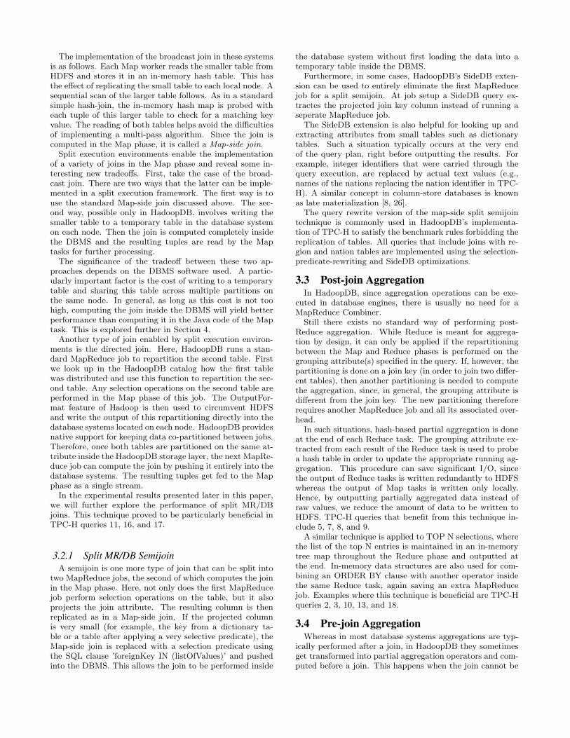
4.6 General ComparisonThe results of benchmarking all three systems are shown

in Figure 3 while the table below presents the numbers (alltimes are in seconds).

First, it is worth noting that DBMS-X significantly out-performs Hive in all queries. This is not surprising, sincethe Hive development team found a similar difference whencomparing their system with DBMS-X [5]. The main rea-son for Hive’s inferior performance is the lack of partitioningand indexing. As a result of this limitation, every selectionbecomes a full data scan and most of the joins involve repar-titioning and shuffling all records across the cluster.

Previous work showed that HadoopDB combined withPostgreSQL was able to approach but not quite reach theperformance level of parallel databases [9]. As a result of

4Chunking slows down the performance slightly, but is nec-essary to maintain HadoopDB’s fault tolerance guarantees[9].

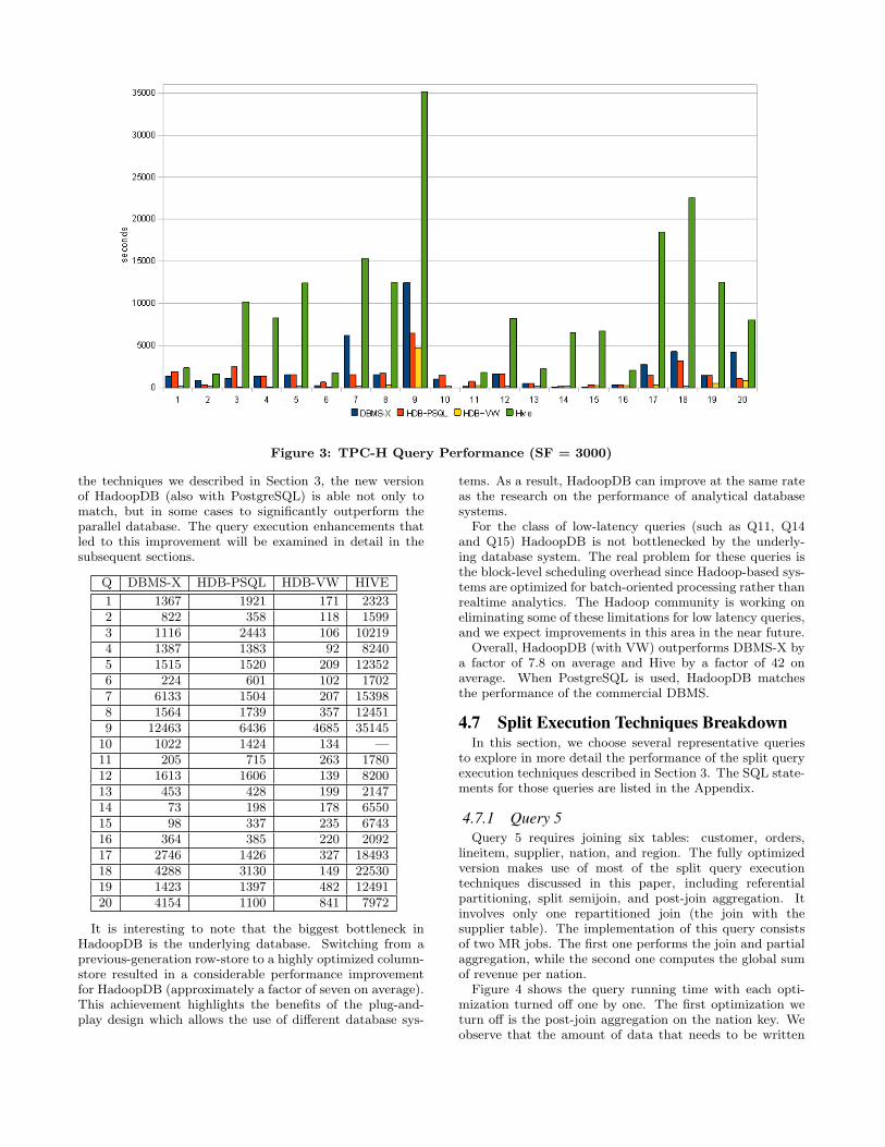
Figure 3: TPC-H Query Performance (SF = 3000)

the techniques we described in Section 3, the new versionof HadoopDB (also with PostgreSQL) is able not only tomatch, but in some cases to significantly outperform theparallel database. The query execution enhancements thatled to this improvement will be examined in detail in thesubsequent sections.

Q DBMS-X HDB-PSQL HDB-VW HIVE

1 1367 1921 171 23232 822 358 118 15993 1116 2443 106 102194 1387 1383 92 82405 1515 1520 209 123526 224 601 102 17027 6133 1504 207 153988 1564 1739 357 124519 12463 6436 4685 35145

10 1022 1424 134 —11 205 715 263 178012 1613 1606 139 820013 453 428 199 214714 73 198 178 655015 98 337 235 674316 364 385 220 209217 2746 1426 327 1849318 4288 3130 149 2253019 1423 1397 482 1249120 4154 1100 841 7972

It is interesting to note that the biggest bottleneck inHadoopDB is the underlying database. Switching from aprevious-generation row-store to a highly optimized column-store resulted in a considerable performance improvementfor HadoopDB (approximately a factor of seven on average).This achievement highlights the benefits of the plug-and-play design which allows the use of different database sys-

tems. As a result, HadoopDB can improve at the same rateas the research on the performance of analytical databasesystems.

For the class of low-latency queries (such as Q11, Q14and Q15) HadoopDB is not bottlenecked by the underly-ing database system. The real problem for these queries isthe block-level scheduling overhead since Hadoop-based sys-tems are optimized for batch-oriented processing rather thanrealtime analytics. The Hadoop community is working oneliminating some of these limitations for low latency queries,and we expect improvements in this area in the near future.

Overall, HadoopDB (with VW) outperforms DBMS-X bya factor of 7.8 on average and Hive by a factor of 42 onaverage. When PostgreSQL is used, HadoopDB matchesthe performance of the commercial DBMS.

4.7 Split Execution Techniques BreakdownIn this section, we choose several representative queries

to explore in more detail the performance of the split queryexecution techniques described in Section 3. The SQL state-ments for those queries are listed in the Appendix.

4.7.1 Query 5Query 5 requires joining six tables: customer, orders,

lineitem, supplier, nation, and region. The fully optimizedversion makes use of most of the split query executiontechniques discussed in this paper, including referentialpartitioning, split semijoin, and post-join aggregation. Itinvolves only one repartitioned join (the join with thesupplier table). The implementation of this query consistsof two MR jobs. The first one performs the join and partialaggregation, while the second one computes the global sumof revenue per nation.

Figure 4 shows the query running time with each opti-mization turned off one by one. The first optimization weturn off is the post-join aggregation on the nation key. Weobserve that the amount of data that needs to be written

Figure 4: Q5 Breakdown for VW Figure 5: Q8 Breakdown for VW Figure 6: Q17 Breakdown for VW

Figure 7: Q5 Breakdown for PSQL Figure 8: Q8 Breakdown for PSQL Figure 9: Q17 Breakdown for PSQL

to HDFS between the two jobs increases from 5.2KB to83.8MB. In an isolated experiment like ours, the effect onquery running time is quite insignificant. The extra I/O be-comes more of a problem in production settings where thereis far more competition for I/O from many concurrent jobs.

The next optimization we turn off is the split semijointechnique (used for the joins of both the customer and sup-plier tables with the nation and region tables). HadoopDBreplaces the split semijoin with a regular Map-side join. Thisresults in a slowdown of about 50% . The reason is that nowthe joins are performed outside of the database system andtherefore cannot take advantage of clustering indices on thenation key.

Finally, we turn off the Map-side join and replace it withthe join done in the Reduce phase. This causes query run-ning time to double. Overall, we reach almost a factor ofthree slowdown versus the fully optimized version. It isworth noting that the entire operation of joining all the ta-bles is still achieved within one MR job, thanks to the factthat the dictionary tables can be brought into memory usingthe SideDB extension.

Turning off optimization techniques has a relativelysmaller effect on HDB-PSQL (Fig. 7) since the totalrunning time is dominated by the slower performingPostgreSQL.

To explore the impact of referential partitioning, we im-plemented in HadoopDB an alternative query execution planwhich assumes only standard partitioning as used in DBMS-X. In this plan, before the join with the supplier table is per-formed, one extra MR job is required to compute the joinbetween the customer and orders/lineitem tables. This ex-tra join causes the total query performance to become slowerby a factor of four versus the layout with referential parti-tioning. The reason is that, internally, that extra job needsto send about 47GB of intermediate data over the networkand write an additional 12GB to HDFS.

4.7.2 Query 8We observe that, like in Query 5, moving the join op-

eration to a later stage within a MapReduce job decreasesperformance. The results are illustrated in Figure 5. Here,employing split semijoin (to restrict nations to the regionof America) gives a speedup by a factor of 2 over the Map-side join and by a factor of 3.6 over the Reduce join. Whenthe less efficient PostgreSQL is used underneath HadoopDB,the contribution of optimization techniques (Fig. 8) is againsmaller.

More specifically, switching to the Map-side join resultedin a total of 5.5M of rows returned by all the databases com-bined (5 times more than in the split semijoin version). Inboth the split semijoin and the regular Map-side join cases,the same amount of intermediate data (around 315GB) iswritten to disk by the Hadoop framework between the Mapand Reduce phases. The amount increases to 1.7TB whenwe perform a repartitioned join in the Reduce phase.

4.7.3 Query 17Query 17 involves a join between the lineitem and part

tables which are not copartitioned. This query would nor-mally involve repartitioning both tables and performing thejoin in Reduce. In Q17, however, very selective predicatesare applied to the part table (69GB of raw data), resulting inonly about 6MB of data (around 600 thousand integer iden-tifiers). This small size gives HadoopDB the opportunityto employ the split MR/DB join technique. Note that thisis not the semijoin version as in the previous two queries,since there are too many values to perform the “foreignKeyIN (listOfValues)” rewrite. Instead, the result of the selec-tion query on the part table is broadcasted to all nodes,and loaded into the database servers where the join is com-puted. In this way, HadoopDB performs the join in the Mapphase, thereby avoiding the repartitioning of the lineitem ta-ble. The gain is about a factor of 2.5 in total running timefor HDB-PSQL and an order of magnitude for HDB-VW.

In order to compare the split MR/DB join technique witha standard Map-side join, we implemented the latter asan alternative execution plan. The results are shown inFigures 6 and 9. Surprisingly, the speedup resulting frompushing the join into the DBMS is greater for VectorWisethan for PostgreSQL. We believe that this is due to thevectorized processing and cache-conscious query executor inVW/X100. PostgreSQL follows the tuple-at-a-time iteratormodel, which results in similar performance as that of theJava hashtable lookups in the Map-side join implementation.Hence, even if the broadcasted table can fit in memory, itmay prove better to write the table to an optimized DBMSand perform the join there, than to perform it in the stan-dard way in the Map phase.

4.8 Analysis of Other Interesting QueriesIn this section we analyze several additional queries that

are notable in some way, usually because they deviate fromour expectations. This helps to further understand the dif-ferent tradeoffs and performance characteristics of the sys-tems.

4.8.1 Query 3Query 3 is similar to Query 5 in that referential parti-

tioning eliminates a significant amount of disk and networkI/O. We expected both HadoopDB combined with Vector-Wise and HadoopDB combined with PostgreSQL to signifi-cantly outperform DBMS-X which does not have the benefitof referential partitioning. This is indeed the case for VW,but the results are quite different for PostgreSQL, as HDB-PSQL is 2 times slower than DBMS-X. A close investigationrevealed that the date predicates are not very selective, re-turning half of the records from both the lineitem and orderstables. Those records need to be joined with about a fifth ofthe rows from the customer table. The PostgreSQL’s EX-PLAIN command indicates that the hash join algorithm isapplied. Given the large number of records, PostgreSQL isnot able to keep all the intermediate data in memory andtherefore needs to swap to disk. In contrast, VectorWiseemploys an efficient merge join algorithm and is able to pro-cesses each chunk without spilling intermediate results todisk.

4.8.2 Query 9This query poses difficulties for each system we bench-

marked. Six tables need to be joined and there is only oneselection predicate (on the part table) to reduce the sizeof the data read from disk. Thus, the query requires shuf-fling most of the data over the network to compute joins.Both HadoopDB setups benefit from pushing three out offive joins into the local databases thanks to the partition-ing of data. VectorWise outperforms PostgreSQL becausethe former is a column-store and in total only 15 out of 46columns need to be read off disk. The column-store advan-tages are somewhat dimished here, however, due to the highcost of tuple reconstruction caused by the large number ofreturned rows.

4.8.3 Query 18In this query HadoopDB with PostgreSQL is about 37%

faster than the parallel database and 7 times more efficientthan Hive. HDB-VW outperforms DBMS-X by a factor of28.8 and Hive by a factor of 151. HadoopDB’s highly ef-

ficient execution plan for this query again benefits greatlyfrom referential partitioning, requiring only one MR job toproduce the desired output. DBMS-X needs to perform onenon-local join (with customer table) but is still able to com-pute the complex subquery in the WHERE clause thanksto partitioning on the order key. Hive first runs an extrajob for that subquery and then joins all tables using therepartitioned join algorithm.

The relatively high difference in performance between theVW/X100 and PostgreSQL setups deserves closer investiga-tion. It turns out that PostgreSQL spends 75% of the timecomputing the subquery responsible for the aggregation ofthe lineitem table via sorting by order key. Due to insuf-ficient memory an external disk merge sort is needed. Incontrast, VW, besides being far more computationally ef-ficient in general, also takes advantage of the fact that thelineitem table is already clustered on the order key attribute.

5. CONCLUSIONWhen the query execution environment is split across

MapReduce and database systems, there appear some inter-esting tradeoffs not present in each system separately. Bycarefully designing HadoopDB’s query engine to operate inthis split execution environment, we achieved a substantialperformance improvement. After equipping HadoopDBwith an efficient single-node columnar DBMS, along withseveral new query execution strategies, we outperformed apopular commercial parallel database system by almost anorder of magnitude, and the state of the art Hadoop-baseddata warehouse by significantly more than an order ofmagnitude. By integrating with Hadoop for job schedulingand network communication, we transformed a single-nodeDBMS into a scalable parallel data analytics platform. Oursystem successfully competes in the most commonly useddata warehouse benchmark against established commercialsolutions.

6. ACKNOWLEDGMENTSThis material is based upon work supported by the Na-

tional Science Foundation under Grant IIS-0844480.

7. REFERENCES[1] Hadapt Inc. Web page. http://www.hadapt.com .

[2] Hadoop. Web page. http://hadoop.apache.org .

[3] Hadoop TeraSort.http://developer.yahoo.com/blogs/hadoop/Yahoo2009.pdf .

[4] Hive. Web page. http://hadoop.apache.org/hive .

[5] Running TPC-H queries on Hive. Web page.http://issues.apache.org/jira/browse/HIVE-600 .

[6] TPC-H. Web page. http://www.tpc.org/tpch .

[7] VectorWise. Web page. http://www.vectorwise.com .

[8] D. J. Abadi, D. S. Myers, D. J. DeWitt, and S. R. Madden.Materialization Strategies in a Column-Oriented DBMS. InICDE, pages 466–475, Istanbul, Turkey, 2007.

[9] A. Abouzeid, K. Bajda-Pawlikowski, D. J. Abadi,A. Silberschatz, and A. Rasin. HadoopDB: An ArchitecturalHybrid of MapReduce and DBMS Technologies for AnalyticalWorkloads. In VLDB, 2009.

[10] A. Abouzied, K. Bajda-Pawlikowski, J. Huang, D. J. Abadi,and A. Silberschatz. Hadoopdb in action: Building real worldapplications. Demonstration. SIGMOD, 2010.

[11] E. Albanese. Why Europe’s Largest Ad Targeting PlatformUses Hadoop. http://www.cloudera.com/blog/2010/03/why-europes-

largest-ad-targeting-platform-uses-hadoop

.

[12] S. Blanas, J. M. Patel, V. Ercegovac, J. Rao, E. J. Shekita,and Y. Tian. A comparison of join algorithms for log

processing in MapReduce. In Proc. of SIGMOD, pages975–986, New York, NY, USA, 2010. ACM.

[13] P. A. Boncz, M. Zukowski, and N. Nes. Monetdb/x100:Hyper-pipelining query execution. In CIDR, pages 225–237,2005.

[14] S. Chen. Cheetah: A High Performance, Custom DataWarehouse on Top of MapReduce. In Proc. of VLDB, 2010.

[15] C. T. Chu, S. K. Kim, Y. A. Lin, Y. Yu, G. R. Bradski, A. Y.Ng, and K. Olukotun. Map-Reduce for Machine Learning onMulticore. In B. Scholkopf, J. C. Platt, and T. Hoffman,editors, NIPS, pages 281–288. MIT Press, 2006.

[16] J. Cohen, B. Dolan, M. Dunlap, J. M. Hellerstein, andC. Welton. MAD skills: new analysis practices for big data.PVLDB, 2(2):1481–1492, 2009.

[17] G. Czajkowski. Sorting 1PB with MapReduce.googleblog.blogspot.com/2008/11/sorting-1pb-with-mapreduce.html .

[18] G. Czajkowski, G. Malewicz, M. Austern, A. Bik, J. Dehnert,I. Horn, and N. Leiser. Pregel: A system for large-scale graphprocessing. In Proc. of SIGMOD, 2010.

[19] J. Dean and S. Ghemawat. MapReduce: Simplified DataProcessing on Large Clusters. In OSDI, 2004.

[20] D. DeWitt and J. Gray. Parallel database systems: the futureof high performance database systems. Commun. ACM,35(6):85–98, 1992.

[21] D. DeWitt and M. Stonebraker. MapReduce: A major stepbackwards. DatabaseColumn Blog.http://databasecolumn.vertica.com/database-innovation/mapreduce-a-

major-step-backwards

.

[22] J. Dittrich, J.-A. Quiane-Ruiz, A. Jindal, Y. Kargin, V. Setty,and J. Schad. Hadoop++: Making a Yellow Elephant Run Likea Cheetah (Without It Even Noticing). In Proc. of VLDB,2010.

[23] G. Eadon, E. I. Chong, S. Shankar, A. Raghavan, J. Srinivasan,and S. Das. Supporting table partitioning by reference inOracle. In Proc. of SIGMOD, pages 1111–1122, 2008.

[24] E. Friedman, P. Pawlowski, and J. Cieslewicz.SQL/MapReduce: a practical approach to self-describing,polymorphic, and parallelizable user-defined functions.PVLDB, 2(2):1402–1413, 2009.

[25] Hadoop. Poweredby. http://wiki.apache.org/hadoop/PoweredBy .

[26] S. Idreos, M. L. Kersten, and S. Manegold. Self-organizingtuple reconstruction in column-stores. In Proc. of SIGMOD,pages 297–308, 2009.

[27] C. Monash. Cloudera presents the MapReduce bull case.DBMS2 Blog.dbms2.com/2009/04/15/cloudera-presents-the-mapreduce-bull-case .

[28] T. Nakayama, M. Hirakawa, and T. Ichikawa. Architecture andAlgorithm for Parallel Execution of a Join Operation. In Proc.of ICDE, pages 160–166, 1984.

[29] B. Panda, J. Herbach, S. Basu, and R. Bayard. PLANET:Massively Parallel Learning of Tree Ensembles withMapReduce. PVLDB, 2(2):1426–1437, 2009.

[30] A. Pavlo, A. Rasin, S. Madden, M. Stonebraker, D. DeWitt,E. Paulson, L. Shrinivas, and D. J. Abadi. A Comparison ofApproaches to Large Scale Data Analysis. In Proc. ofSIGMOD, 2009.

[31] A. Thusoo, J. S. Sarma, N. Jain, Z. Shao, P. Chakka,

N. Zhang, S. Antony, H. Liu, and R. Murth. Hive U A PetabyteScale Data Warehouse Using Hadoop. In Proc. of ICDE, 2010.

[32] R. Vernica, M. Carey, and C. Li. Efficient ParallelSet-Similarity Joins Using MapReduce. In Proc. of SIGMOD,2010.

[33] C. Yang, C. Yen, C. Tan, and S. Madden. Osprey:Implementing MapReduce-Style Fault Tolerance in aShared-Nothing Distributed Database. In ICDE ’10, 2010.

[34] H.-c. Yang, A. Dasdan, R.-L. Hsiao, and D. S. Parker.Map-reduce-merge: simplified relational data processing onlarge clusters. In Proc. of SIGMOD, pages 1029–1040, 2007.

[35] M. Zukowski. Balancing Vectorized Query Execution withBandwidth-Optimized Storage. PhD thesis, Universiteit vanAmsterdam, Amsterdam, The Netherlands, 2009.

APPENDIXTPC-H Query 3

select first 10

l_orderkey, sum(l_extendedprice * (1 - l_discount)) as revenue,

o_orderdate, o_shippriority

from

customer, orders, lineitem

where

c_mktsegment = ’BUILDING’

and c_custkey = o_custkey

and l_orderkey = o_orderkey

and o_orderdate < date ’1995-03-15’

and l_shipdate > date ’1995-03-15’

group by

l_orderkey, o_orderdate, o_shippriority

order by

revenue desc, o_orderdate

TPC-H Query 5

select

n_name, sum(l_extendedprice * (1 - l_discount)) as revenue

from

customer, orders, lineitem, supplier, nation, region

where

c_custkey = o_custkey

and l_orderkey = o_orderkey

and l_suppkey = s_suppkey

and c_nationkey = s_nationkey

and s_nationkey = n_nationkey

and n_regionkey = r_regionkey

and r_name = ’ASIA’

and o_orderdate >= date ’1994-01-01’

and o_orderdate < date ’1994-01-01’

+ interval ’1’ year

group by

n_name

order by

revenue desc

TPC-H Query 7

select

supp_nation, cust_nation, l_year, sum(volume) as revenue

from

(

select

n1.n_name as supp_nation, n2.n_name as cust_nation,

extract(year from l_shipdate) as l_year,

l_extendedprice * (1 - l_discount) as volume

from

supplier, lineitem, orders, customer, nation n1, nation n2

where

s_suppkey = l_suppkey

and o_orderkey = l_orderkey

and c_custkey = o_custkey

and s_nationkey = n1.n_nationkey

and c_nationkey = n2.n_nationkey

and (

(n1.n_name = ’FRANCE’ and n2.n_name = ’GERMANY’)

or (n1.n_name = ’GERMANY’ and n2.n_name = ’FRANCE’)

)

and l_shipdate between date ’1995-01-01’

and date ’1996-12-31’

) as shipping

group by

supp_nation, cust_nation, l_year

order by

supp_nation, cust_nation, l_year

TPC-H Query 8

select

o_year, sum(case when nation = ’BRAZIL’ then volume

else 0 end) / sum(volume) as mkt_share

from

(

select

extract(year from o_orderdate) as o_year,

l_extendedprice * (1 - l_discount) as volume,

n2.n_name as nation

from

part, supplier, lineitem, orders,

customer, nation n1, nation n2, region

where

p_partkey = l_partkey

and s_suppkey = l_suppkey

and l_orderkey = o_orderkey

and o_custkey = c_custkey

and c_nationkey = n1.n_nationkey

and n1.n_regionkey = r_regionkey

and r_name = ’AMERICA’

and s_nationkey = n2.n_nationkey

and o_orderdate between date ’1995-01-01’

and date ’1996-12-31’

and p_type = ’ECONOMY ANODIZED STEEL’

) as all_nations

group by

o_year

order by

o_year

TPC-H Query 9

select

nation, o_year, sum(amount) as sum_profit

from

(

select

n_name as nation,

extract(year from o_orderdate) as o_year,

l_extendedprice * (1 - l_discount)

- ps_supplycost * l_quantity as amount

from

part, supplier, lineitem, partsupp, orders, nation

where

s_suppkey = l_suppkey

and ps_suppkey = l_suppkey

and ps_partkey = l_partkey

and p_partkey = l_partkey

and o_orderkey = l_orderkey

and s_nationkey = n_nationkey

and p_name like ’%green%’

) as profit

group by

nation, o_year

order by

nation, o_year desc

TPC-H Query 17

select

sum(l_extendedprice) / 7.0 as avg_yearly

from

lineitem, part

where

p_partkey = l_partkey

and p_brand = ’Brand#23’

and p_container = ’MED BOX’

and l_quantity < (

select

0.2 * avg(l_quantity)

from

lineitem

where

l_partkey = p_partkey

)

TPC-H Query 18

select first 100

c_name, c_custkey, o_orderkey,

o_orderdate, o_totalprice, sum(l_quantity)

from

customer, orders, lineitem

where

o_orderkey in (

select

l_orderkey

from

lineitem

group by

l_orderkey

having

sum(l_quantity) > 300

)

and c_custkey = o_custkey

and o_orderkey = l_orderkey

group by

c_name, c_custkey, o_orderkey, o_orderdate, o_totalprice

order by

o_totalprice desc, o_orderdate

TPC-H Query 20

select

s_name, s_address

from

supplier, nation

where

s_suppkey in (

select

ps_suppkey

from

partsupp

where

ps_partkey in (

select

p_partkey

from

part

where

p_name like ’forest%’

)

and ps_availqty > (

select

0.5 * sum(l_quantity)

from

lineitem

where

l_partkey = ps_partkey

and l_suppkey = ps_suppkey

and l_shipdate >= date ’1994-01-01’

and l_shipdate < date ’1994-01-01’

+ interval ’1’ year

)

)

and s_nationkey = n_nationkey

and n_name = ’CANADA’

order by

s_name