efﬁcient processing of large graphs via input...

Efficient Processing of Large Graphs via Input Reduction

1Amlan Kusum 1Keval Vora 1Rajiv Gupta 2Iulian Neamtiu

1Department of Computer Science, University of California, Riverside{akusu001, kvora001, gupta}@cs.ucr.edu

2Department of Computer Science, New Jersey Institute Of [email protected]

ABSTRACTLarge-scale parallel graph analytics involves executing iter-ative algorithms (e.g., PageRank, Shortest Paths, etc.) thatare both data- and compute-intensive. In this work we con-struct faster versions of iterative graph algorithms from theiroriginal counterparts using input graph reduction. A largeinput graph is transformed into a small graph using a se-quence of input reduction transformations. Savings in execu-tion time are achieved using our two phased processing modelthat effectively runs the original iterative algorithm in twophases: first, using the reduced input graph to gain savingsin execution time; and second, using the original input graphalong with the results from the first phase for computingprecise results. We propose several input reduction transfor-mations and identify the structural and non-structural prop-erties that they guarantee, which in turn are used to ensurethe correctness of results while using our two phased pro-cessing model. We further present a unified input reductionalgorithm that efficiently applies a non-interfering sequenceof simple local input reduction transformations. Our ex-periments show that our transformation techniques enablesignificant reductions in execution time (1.25×-2.14×) whileachieving precise final results for most of the algorithms. Forcases where precise results cannot be achieved, the relativeerror remains very small (at most 0.065).

CCS Concepts•Computing methodologies→ Parallel computingmethodologies; Parallel programming languages;

KeywordsGraph Processing; Input Reduction; Iterative Algorithms

1. INTRODUCTIONWith the proliferation of data, parallel graph analytics

has become a difficult task because it involves executing it-erative algorithms on very large graphs. This has led re-searchers to explore acceleration strategies, some of whichproduce approximate results. There are two main strategies

Permission to make digital or hard copies of all or part of this work for personal orclassroom use is granted without fee provided that copies are not made or distributedfor profit or commercial advantage and that copies bear this notice and the full cita-tion on the first page. Copyrights for components of this work owned by others thanACM must be honored. Abstracting with credit is permitted. To copy otherwise, or re-publish, to post on servers or to redistribute to lists, requires prior specific permissionand/or a fee. Request permissions from [email protected].

HPDC’16, May 31-June 04, 2016, Kyoto, Japanc© 2016 ACM. ISBN 978-1-4503-4314-5/16/05. . . $15.00

DOI: http://dx.doi.org/10.1145/2907294.2907312

for approximate computing: algorithmic [5, 18, 1] and code-centric [21, 20, 29, 25, 2, 27]. The algorithmic approachis application specific and thus the ideas for one applica-tion may not transfer to others. The code-centric approachtransforms the application so that at runtime it switchesbetween code versions or skips computations to save time,albeit sacrificing accuracy. However, for applications whosebehavior is input sensitive, intelligent skipping is difficult asthe program lacks global view of input characteristics.

In this paper we present a general approach for acceler-ating parallel vertex-centric iterative graph algorithms thatrepeatedly process large graphs until convergence. Eventhough these algorithms are parallel, their execution timescan be large for real-world inputs. Thus there is a greatdeal of benefit in approximating them to save processingtime. The novel aspect of our two-phased approach is thatit is input data-centric. In the first phase, the original (un-changed) iterative algorithm is applied on a smaller graphwhich is representative of the original large input graph; thisstep yields savings in execution time. In the second phase,the results from the smaller graph are transferred to the orig-inal larger graph and, via application of the original graphalgorithm, error reduction is achieved, possibly convergingto the final accurate results. The additional time requiredto process the reduced graph in the first phase (Tphase1)pays off as it is significantly lower than the savings achievedby the second phase (Toriginal − Tphase2); hence the overallprocessing time reduces from Toriginal to Tphase1 + Tphase2.

To reduce the size of input graphs, we propose light-weightvertex-level input reduction transformations whose applica-tion is guided by their impact on graph connectivity (i.e., theglobal structure of the graph). While there exist works [7,17, 3, 18, 23, 35, 9, 8, 10] that reduce the size of graphs toaccelerate processing, they mainly present algorithm-specificreduction techniques and mostly operate of regular meshes.[7, 17] present a multilevel graph partitioning algorithmwhere first a hierarchy of smaller graphs is created, thenthe highest level graphs are partitioned and then, these par-tition results are carefully propagated back down the hier-archy to achieve partitioning of the original graph. Theyuse edge contraction or maximal independent set computa-tion over dual graph which are suitable for relatively regularmesh structures but can be computationally expensive. [3,9, 8, 10] also partition graphs via recursive edge contrac-tion using maximal independent set computation to generatemultinodes. In contrast, we identify light-weight, local andnon-interfering transformations which are general (i.e., notalgorithm-specific) and are suitable for reducing large irreg-

http://dx.doi.org/10.1145/2907294.2907312

ular input graphs. Moreover, our reduction strategy is nothierarchical (multi-level) since our transformations are de-signed from the vertex’s perspective and are applied at mostonce on each vertex. Other works like [23, 35] are specif-ically designed for certain problems (e.g., shortest paths)and require path-level or component-level transformationsthat involve computationally intensive pre-processing. Ourtransformations are vertex-level, light-weight, ans suitablefor large irregular graphs.

Upon carefully studying various characteristics of vertexcentric algorithms and properties of input reduction trans-formations, we show that it is possible to achieve fully accu-rate results for a subclass of graph algorithms, while remain-ing algorithms produce approximate solutions. In compari-son to algorithmic works our approach is more general andin contrast to code-centric our approach has two advantages:

– Input Data-centric Approximation: via graph reduction,we achieve the effect of skipping computations like the code-centric approach. However, since skipping is achieved as aconsequence of input graph reduction that is performed asa preprocessing phase, the decision of what to skip is sensi-tive to the structure of the input graph – graph connectivityguides the application of transformations.

– Uncompromised Processing Algorithm: our approach re-quires no changes to the core graph analysis algorithm. Theoriginal algorithm is used until convergence on the reducedgraph and then on the full graph for error reduction. Withcareful choice of input transformations, the algorithm’s ca-pability can remain uncompromised, i.e., upon convergencethe error reduction phase can give precise results.

We evaluate our two-phased processing technique in ashared memory environment using Galois [19], a state-of-the-art parallel execution and graph processing framework.Our experiments with six graph algorithms and multiplereal-world graphs show that our techniques achieve an av-erage speedup of 1.25×-2.14× while achieving precise finalresults for five benchmarks and approximate results for onewith very low relative error (at most 0.065).

2. OVERVIEW OF OUR APPROACHThis section provides an overview of our two phased pro-

cessing model. While graph reduction based processing strat-egies are used in various works like [7, 17], we focus on it-erative general purpose graph algorithms and operate on asingle reduced graph along with the original input graph(i.e., there are no multiple levels in the hierarchy). Weuse the vertex-centric programming model as it is intuitiveand commonly used by many graph processing systems likeGraphLab [15], GraphX [34], and Galois [19]. We considerdirected graphs in our discussion; our approach easily sim-plifies to handle undirected graphs.

Given an iterative vertex-centric graph algorithm iA anda large input graph G, the accurate results of vertex valuesVG can be computed by applying iA to G, that is:

VG = iA(G)

To accelerate this computation, we use the following steps:

• Reduce input G to G′: we transform the large inputgraph G into a smaller graph G′ via multiple appli-cations of an input reduction transformation T .

• Compute results for G′: we apply iA to G′ to computeVG′ . Computing on VG′ takes lesser time than on VG .

• Obtain results for G: using simple mapping rules mRs,we convert the results VG′ to V 1

G . Then, via multipleapplication of update rules in iA, we reduce the errorin V 1

G and obtain the result V 2G .

Thus, our approach replaces computation VG = iA(G) by:

[INPUT REDUCTION] G′ = T ∆(G)[PHASE 1] VG′ = iA (G′)[MAP RESULTS] mR : VG′ → V 1

G[PHASE 2] V 2

G = iA (V 1G , G)

where ∆ is a parameter that controls the degree of reductionperformed as it represents the number of applications of Tto G. Thus, the greater the value of ∆, the smaller the sizeof the reduced graph G′. Depending on various propertiesof input reduction transformations T (Section 3.2) and thenature of iterative algorithm iA, the computed values willbe accurate, i.e., V 2

G = VG . However, we identify cases inwhich V 2

G may not be the same as VG (Section 4) — thecomputed results are approximate for those cases.

2.1 Efficient Input Reduction TransformationsGiven the iterative nature of algorithms considered, ap-

plying iA to G′ as opposed to G is expected to result in ex-ecution time savings. However, these savings can be offsetby the extra overhead due to application of input reductiontransformations and result converting rules. Therefore wemust ensure that these steps are simpler than the iterativecomputation that they aim to avoid. We do so by placingthe following restrictions on the kind of transformation thatis allowed (local) and the sequence of its application (non-interfering) permitted for reducing G to G′.A. Local transformation. Transformation T (v,G), wherev is a vertex in G, is a local transformation if its applicationonly examines edges directly connected to v. The subgraphinvolving v and its edges is denoted as subGraph(T (v,G)).

G1 ← T (v1,G); G2 ← T (v2,G1) · · ·· · · G∆−1 ← T (v∆−1,G∆−2); G′ ← T (v∆,G∆−1)

B. Non-interfering sequence. T ∆, a sequence of ∆ ap-plications of local transformation T as shown above is non-interfering if and only if: vertices v1 · · · v∆ are distinct ver-tices in G; and each subGraph(T (vi,G)) is contained in G.Note that the above restrictions (local and non-interfering)ensure that input reduction is performed via a single passover the original graph because:

• An edge vi → vj from G is only examined when con-sidering the application of T to vi or vj ; and

• Any vertex or edge created during one application ofT cannot be involved in any other application of T .

Thus, the cost of applying the transformation sequence islinear in the size of G, i.e., the number of vertices and edgesin it. Moreover, the cost of converting results is proportionalto the size of the transformed portions of G. In contrast,those computations over the transformed portions of G thatwe avoid would have required repeated passes due to theiterative nature of graph algorithms considered.

In conclusion, the restrictions on transformations and se-quences ensure that the cost of applying them will be lessthan the cost of the computation they avoid, leading to netsavings in execution time.

Algorithm 1 Iterative Vertex-Centric Graph Algorithm.

1: function TPiA ( input G )2: G′ ← ReduceGraph ( G, T , ∆ )3: V 1

G ← iA(G′)4: V 2

G ← iAP2(V 1G , G)

5: return V 2G

6: end function

7: function ReduceGraph ( G, T , ∆ )8: G′ ← G9: for ( Vertex v : G ) do

10: if ( NI ( subGraph(T (v,G)) ) then11: G′ ← T (v,G′)12: ∆← ∆− 113: if ( ∆ == 0 ) then break end if14: end if15: end for16: return G′17: end function

18: function iA ( input G )19: Initialize VG & WorkQ20: while ( ! WorkQ.empty ) do21: v ← WorkQ.getFirst()22: if ( UpdateVals (v, VG) ) then23: WorkQ.add ( outNeighbors (v) )24: end if25: end while26: return VG27: end function

28: function UpdateVals ( v, VG )29: Updated ← false30: if updateCheck ( v, inNeighbors (v) ) then31: update VG [v]32: Updated ← true33: end if34: return Updated35: end function

36: function iAP2 ( V 1G , G )

37: Initialize WorkQ38: for ( Vertex v : G ) do39: if ( v ∈ G′ ) then40: V 2

G ( v ) ← V 1G (v)

41: else42: V 2

G ( v ) ← initval ( )43: WorkQ.add ( v )44: end if45: end for46: WorkQ.add ( Vertex v s.t. v is affected by47: addition / deletion of edges)48: while ( ! WorkQ.empty ) do49: v ← WorkQ.getFirst()50: if ( UpdateVals (v, VG) ) then51: WorkQ.add ( outNeighbors (v) )52: end if53: end while54: return VG55: end function

Algorithm 2 SSSP Algorithm.

1: function TwoPhaseSSSP ( input G; srcVertex )2: � VG of a vertex v = length of the3: � shortest path from srcVertex to v4: end function

5: function ReduceGraph ( G, T , ∆, srcVertex )6: � srcVertex is not part of applied T ’s7: end function

8: function InitializeSSSP ( input G; srcVertex )9: � Initialize VG

10: for ( Vertex v : G ) do VG [v] ← ∞11: end for12: VG [srcVertex] ← 013: � Initialize WorkQ14: WorkQ.add( outNeighbors(srcVertex) )15: end function

16: function UpdateVals ( v, VG )17: Updated ← false18: for ( Vertex v′ : inNeighbors (v) ) do19: if VG [v] > VG [v′] + wt(v′, v) then20: VG [v] ← VG [v′] + wt(v′, v)21: Updated ← true22: end if23: end for24: return Updated25: end function

26: function Phase2SSSP ( VG′ , G )27: initval() assigns ∞ or results from phase 128: end function

2.2 Original and Two-Phased AlgorithmsNext we summarize our approach by presenting the gen-

eral form of an original iterative vertex-centric graph algo-rithm and its corresponding two phased version. In Algo-rithm 1, function iA represents the original algorithm whoseapplication to graph G produces the accurate (VG) result.Function TPiA is the two phased version that calls iA andiAP2 in first and second phases. Note that the processinglogic in iAP2 (lines 48-53) is exactly the same as that in iA

(lines 20-25). The result (V 2G ) is obtained from the applica-

tion of TPiA to G. The result obtained from TPiA might notbe accurate; we discuss this in Sections 4.1 and 4.2.

ReduceGraph examines the vertices in G one at a time andif T (v,G′) is non-interfering with transformations alreadyapplied, then it is applied on v. The function NI enforcesnon-interference by ensuring that all vertices and edges insubGraph(T (v,G)) are being examined for the first time.The algorithm terminates after applying ∆ transformations.The function iAP2 copies results from vertices in G′ to ver-tices in G for each vertex that is present in both graphs. Thevertices in G that were eliminated in the process of creatingG′ are assigned initial values by initval(). Then, similarto iA, UpdateVals is applied to V 2

G until convergence.

2.3 Example: Single Source Shortest PathsAlgorithm 2 presents the two-phased version of the Single

Source Shortest Paths (SSSP) algorithm. Only the code se-quences that are specific to SSSP are shown while other codesequences from Algorithm 1 remain the same. The functionUpdateVals() computes the shortest path for a vertex vbased on its incoming edges.

f

s

cd

a

bge

1

1

1

1

2

3

4

63

32

1

1

(a) Original G.

s

cd

a

b

2

1

63

2

1

(b) Transformed G′.Figure 1: Graph reduction example.

s

cd

a

b

2

1

632

1

2 23

90

(a) VG′ computed - 1st phase.

f

s

cd

a

bge

1

1

1

1

2

3

4

6332

1

1

0 9

2 2 3

∞∞∞

(b) V 1G initialized from VG′

f

s

cd

a

bge

1

1

1

1

2

3

4

6332

1

1

0 9

2 2 3

∞11

(c) V 2G computed - 2nd phase.

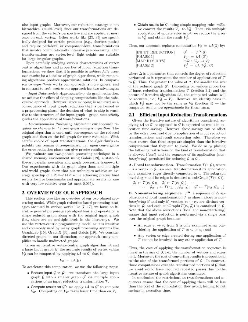
Figure 2: Two-phased SSSP processing on G & G′.Figure 1 illustrates graph reduction by converting G toG′ and Figure 2 illustrates how the two-phased SSSP algo-rithm works on the example graph by first computing VG′(Figure 2-a), then feeding these computed results to V 1

G (Fig-ure 2-b), and then computing V 2

G (Figure 2-c). In this case asingle application of UpdateVals in the second phase yieldsprecise results (i.e., V 2

G = VG). In general, for large com-plex graphs and different applications, this may not be thecase; however, the results computed in the first phase willaccelerate the second phase.

3. INPUT REDUCTIONWe present six transformations to reduce input graph and

discuss their properties to gain useful programming insights.

3.1 Transformations for Input ReductionSince many graph algorithms are super-linear in the num-

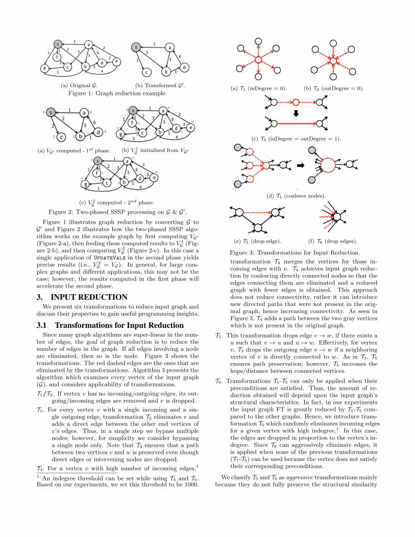
ber of edges, the goal of graph reduction is to reduce thenumber of edges in the graph. If all edges involving a nodeare eliminated, then so is the node. Figure 3 shows thetransformations. The red dashed edges are the ones that areeliminated by the transformations. Algorithm 3 presents thealgorithm which examines every vertex of the input graph(G), and considers applicability of transformations.

T1/T2. If vertex v has no incoming/outgoing edges, its out-going/incoming edges are removed and v is dropped.

T3. For every vertex v with a single incoming and a sin-gle outgoing edge, transformation T3 eliminates v andadds a direct edge between the other end vertices ofv’s edges. Thus, in a single step we bypass multiplenodes; however, for simplicity we consider bypassinga single node only. Note that T3 ensures that a pathbetween two vertices v and w is preserved even thoughdirect edges or intervening nodes are dropped.

T4. For a vertex v with high number of incoming edges,1

1 An indegree threshold can be set while using T4 and T6.Based on our experiments, we set this threshold to be 1000.

(a) T1 (inDegree = 0). (b) T2 (outDegree = 0).

(c) T3 (inDegree = outDegree = 1).

(d) T4 (coalesce nodes).

(e) T5 (drop edge). (f) T6 (drop edges).

Figure 3: Transformations for Input Reduction.

transformation T4 merges the vertices for those in-coming edges with v. T4 achieves input graph reduc-tion by coalescing directly connected nodes so that theedges connecting them are eliminated and a reducedgraph with fewer edges is obtained. This approachdoes not reduce connectivity, rather it can introducenew directed paths that were not present in the orig-inal graph, hence increasing connectivity. As seen inFigure 3, T4 adds a path between the two gray verticeswhich is not present in the original graph.

T5. This transformation drops edge v → w, if there exists au such that v → u and u → w. Effectively, for vertexv, T3 drops the outgoing edge v → w if a neighboringvertex of v is directly connected to w. As in T3, T5

ensures path preservation; however, T5 increases thehops/distance between connected vertices.

T6. Transformations T1-T5 can only be applied when theirpreconditions are satisfied. Thus, the amount of re-duction obtained will depend upon the input graph’sstructural characteristics. In fact, in our experimentsthe input graph FT is greatly reduced by T1-T5 com-pared to the other graphs. Hence, we introduce trans-formation T6 which randomly eliminates incoming edgesfor a given vertex with high indegree.1 In this case,the edges are dropped in proportion to the vertex’s in-degree. Since T6 can aggressively eliminate edges, itis applied when none of the previous transformations(T1-T5) can be used because the vertex does not satisfytheir corresponding preconditions.

We classify T5 and T6 as aggressive transformations mainlybecause they do not fully preserve the structural similarity

Algorithm 3 Graph Reduction Algorithm.

1: Algorithm TRANSFORM ( G(V, E) )2: E ′ ← E3: for ∀v ∈ V do4: if ( inDegree(v) = 0 ) then5: � apply T1 : drop v → ∗6: E ′ ← E ′\ outEdges(v)7: elseif ( outDegree(v) = 0 ) then8: � apply T2 : drop ∗ → v9: E ′ ← E ′\ inEdges(v)

10: elseif ( inDegree(v) = outDegree(v) = 1 ) then11: � apply T3 : bypass v12: E ′ ← (E ′ \ {u→ v, v → w}) ∪ {u→ w}13: where {u→ v, v → w} ⊆ E ′14: elseif ( all inNeighbors(v) are unchanged ) then15: � apply T4 : coalesce v and inNeighbors(v)16: E ′ ← coalesce(G, E ′, v)17: end if18: end for19: if ( G requires further reduction ) then20: for ∀v ∈ V s.t. v is unchanged do21: if ( w ∈ outNeighbors(v) s.t. w is unchanged and22: outNeighbors(v) ∩ inNeighbors(w) 6= φ ) then23: � apply T5 : drop v → w24: E ′ ← E ′ \ {(v → w)}25: elseif ( inDegree(v) > threshold ) then26: � apply T6 : drop some ∗ → v27: E ′ ← E ′ \R where R ⊆ inEdges(v)28: end if29: end for30: end if31: return E ′ of G′32: end algorithm33:34: Algorithm COALESCE ( G(V, E), E ′, v )35: for ∀(w → v) ∈ inEdges(v) do36: E ′ ← E ′ \ {w → v}37: for ∀(u→ w) ∈ inEdges(w) do38: E ′ ← E ′ \ {u→ w}39: E ′ ← E ′ ∪ {u→ v}40: end for41: for ∀(w → u) ∈ outEdges(w) do42: E ′ ← E ′ \ {w → u}43: E ′ ← E ′ ∪ {v → u}44: end for45: end for46: return E ′ of G′47: end algorithm

between the transformed graph and the original graph. Inparticular, T5 can effectively increase the diameter of the in-put graph by spreading out vertices which are close to eachother in the original graph, far apart in the transformedgraph and hence, increasing the traversal cost. T6, on theother hand, randomly drops edges from high-degree verticeswhich are typically important locations defining the graphstructure. Care must be taken while reducing the graph us-ing these transformations since the computed values fromfirst phase using structurally dissimilar graphs can prove tobe useless and hence, demand significant computation on theoriginal graph in the second phase. Algorithm 3 achieves ourobjective of applying a non-interfering sequence of transfor-

Trans.

[V-ADD]

[V-SUB]

[E-ADD]

[E-SUB]

[C-M

ERGE]

[C-SPLIT]

T1 7 3 7 3 7 ?T2 7 3 7 3 7 ?T3 7 3 3 3 7 7T4 7 3 3 3 7 7T5 7 7 7 3 7 7

T6 7 7 7 3 7 ?

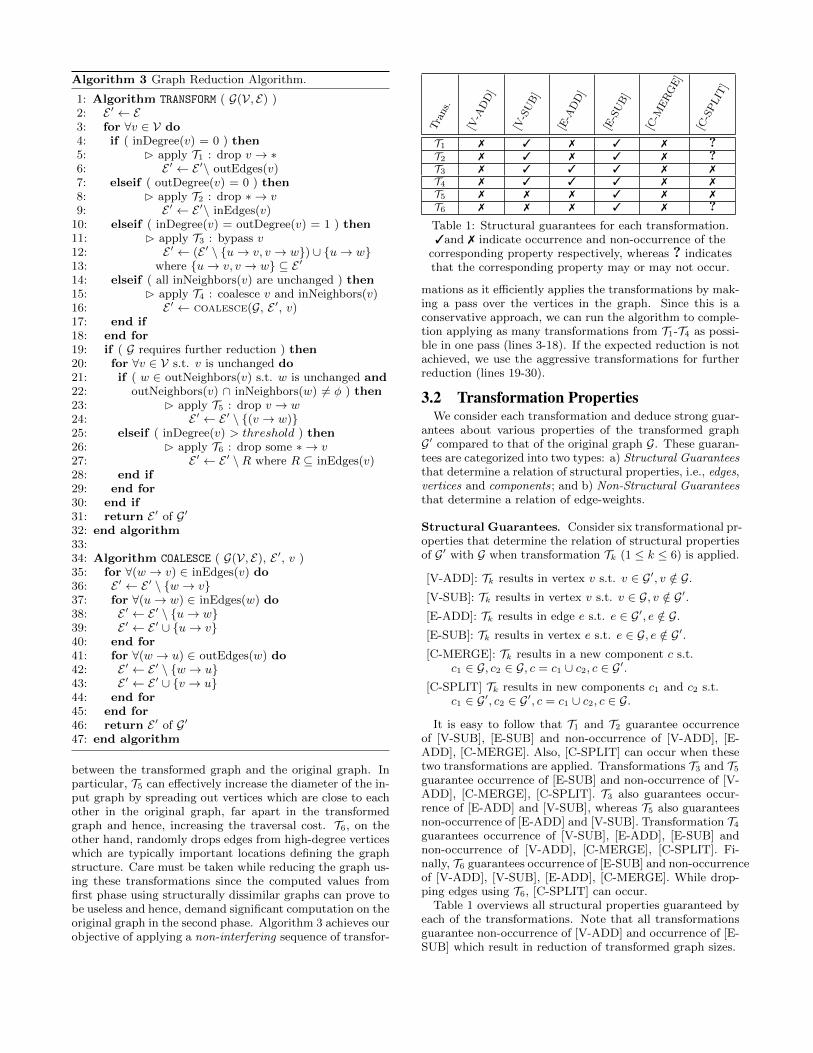
Table 1: Structural guarantees for each transformation.3and 7 indicate occurrence and non-occurrence of the

corresponding property respectively, whereas ? indicatesthat the corresponding property may or may not occur.

mations as it efficiently applies the transformations by mak-ing a pass over the vertices in the graph. Since this is aconservative approach, we can run the algorithm to comple-tion applying as many transformations from T1-T4 as possi-ble in one pass (lines 3-18). If the expected reduction is notachieved, we use the aggressive transformations for furtherreduction (lines 19-30).

3.2 Transformation PropertiesWe consider each transformation and deduce strong guar-

antees about various properties of the transformed graphG′ compared to that of the original graph G. These guaran-tees are categorized into two types: a) Structural Guaranteesthat determine a relation of structural properties, i.e., edges,vertices and components; and b) Non-Structural Guaranteesthat determine a relation of edge-weights.

Structural Guarantees. Consider six transformational pr-operties that determine the relation of structural propertiesof G′ with G when transformation Tk (1 ≤ k ≤ 6) is applied.

[V-ADD]: Tk results in vertex v s.t. v ∈ G′, v /∈ G.

[V-SUB]: Tk results in vertex v s.t. v ∈ G, v /∈ G′.[E-ADD]: Tk results in edge e s.t. e ∈ G′, e /∈ G.

[E-SUB]: Tk results in vertex e s.t. e ∈ G, e /∈ G′.[C-MERGE]: Tk results in a new component c s.t.

c1 ∈ G, c2 ∈ G, c = c1 ∪ c2, c ∈ G′.[C-SPLIT] Tk results in new components c1 and c2 s.t.

c1 ∈ G′, c2 ∈ G′, c = c1 ∪ c2, c ∈ G.

It is easy to follow that T1 and T2 guarantee occurrenceof [V-SUB], [E-SUB] and non-occurrence of [V-ADD], [E-ADD], [C-MERGE]. Also, [C-SPLIT] can occur when thesetwo transformations are applied. Transformations T3 and T5

guarantee occurrence of [E-SUB] and non-occurrence of [V-ADD], [C-MERGE], [C-SPLIT]. T3 also guarantees occur-rence of [E-ADD] and [V-SUB], whereas T5 also guaranteesnon-occurrence of [E-ADD] and [V-SUB]. Transformation T4

guarantees occurrence of [V-SUB], [E-ADD], [E-SUB] andnon-occurrence of [V-ADD], [C-MERGE], [C-SPLIT]. Fi-nally, T6 guarantees occurrence of [E-SUB] and non-occurrenceof [V-ADD], [V-SUB], [E-ADD], [C-MERGE]. While drop-ping edges using T6, [C-SPLIT] can occur.

Table 1 overviews all structural properties guaranteed byeach of the transformations. Note that all transformationsguarantee non-occurrence of [V-ADD] and occurrence of [E-SUB] which result in reduction of transformed graph sizes.

Non-Structural Guarantees. Since transformations T3

and T4 guarantee occurrence of [E-ADD], correct edge weightsneed to be assigned to newly added edges for weighted graphs.We define two transformational properties which determinethe relation of edge weights of G′ with that of G when trans-formation Tk (1 ≤ k ≤ 6) is applied. In the following ex-pressions, a =⇒ b means b ∈ G′ is resulted from a ∈ G.

[E-EQUAL] Tk results in edges e1 and e2, both with weightsw(e) s.t. e1 ∈ G, e1 /∈ G′, e2 ∈ G′, e2 /∈ G, e1 =⇒ e2.

[E-FUNC] Tk results in edges e1, e2 and e3, with weightsw(e1), w(e2) and w(e3) respectively s.t.{e1, e2} ∈ G, {e1, e2} /∈ G′, e3 ∈ G′, e3 /∈ G,w(e3) = func(w(e1), w(e2)), (e1, e2) =⇒ e3.

[E-FUNC] represents the weight of the newly added edge asa function of weights of edges from the original graph thatresulted in this new edge. For example, the new weight canbe set as the sum, minimum, or maximum of the originaledge weights ([E-SUM], [E-MIN], or [E-MAX] respectively).

Transformation T3 guarantees occurrence of [E-FUNC] andnon-occurrence of [E-EQUAL]. For transformation T4, both[E-EQUAL] and [E-FUNC] can occur. As we will see inSection 4.1, we use [E-SUM] to benefit the exploratory andtraversal based graph algorithms.

4. PROGRAMMING FOR TRANSFORMEDGRAPHS

Using the transformation properties described in Section 3.2,we discuss properties of vertex-centric graph algorithms thatpermit them to benefit from the two-phased model.

4.1 Impact of Transformationson Vertex Functions

Since the aforementioned transformations change the struc-tural and non-structural properties of the graph, it is impor-tant to determine the impact of these changes on how pro-grammers should correctly express graph algorithms. Eventhough custom algorithms can be written so that computa-tions performed on transformed graphs always lead to cor-rect values, we eliminate this programming overhead by sup-porting the popular vertex centric programming for our twophased processing model.

Vertex-centric programming. In this model, algorithmsare expressed in a vertex-centric manner, i.e., computationsare written from the perspective of a single vertex. Thesecomputations, called vertex functions, are iteratively exe-cuted on all vertices in parallel, until all the vertex values inthe graph stabilize. Vertex functions typically use the valuescoming from its incoming edges as inputs for computation.Hence, the newly computed value of a vertex depends onthe values coming from its incoming edges. Moreover, theasynchronous nature of the graph algorithms requires com-putations over updates coming from incoming edges to becommutative and associative — this way, updates comingfrom different incoming edges can be processed in any or-der, e.g., the order of their arrival.

To guarantee correct answers at the end of computation,we need to reason about the behavior of vertex functions,first when applied on the transformed graph G′, and lateron the original graph G. For illustration, we use two ver-sions of the SSSP vertex functions, SSSP-IN and SSSP-SIN,

Algorithm 4 Variants of SSSP vertex functions.

1: function SSSP-IN ( Vertex v )2: if ( v = source ) return 0; end if3: minPath←∞4: for ( Vertex u : inNeighbors (v) ) do5: if ( u.path+ wt(u,w) < minPath ) then6: minPath← u.path+ wt(u,w)7: end if8: end for9: return minPath

10: end function11:12: function SSSP-SIN ( Vertex v )13: if ( v = source ) return 0; end if14: minPath← v.path15: for ( Vertex u : inNeighbors (v) ) do16: if ( u.path+ wt(u,w) < minPath ) then17: minPath← u.path+ wt(u,w)18: end if19: end for20: return minPath21: end function

shown in Algorithm 4. Computations in SSSP-IN only de-pend on values coming from incoming neighbors, whereasthose in SSSP-SIN depends on the previous value of the ver-tex in addition to the values coming from neighbors. Theonly difference between SSSP-IN and SSSP-SIN is the ini-tialization of minPath (line 3 and 14 marked in red); therest of the functions are identical. Note that both of thesevariants produce correct results when used in the traditionalvertex centric processing model. However, they behave dif-ferently when used in our two-phased processing model, inwhich only SSSP-IN leads to accurate results.

Let us evaluate each of the structural and non-structuralproperties which are affected by our transformations.

(A) [V-SUB] and [E-SUB]: [E-SUB] leads to compu-tations being performed even when all the incoming edgesof a vertex are not available. Such computations are equiva-lent to that in the staleness-based (i.e., relaxed consistency)computation model [31] where the edges can potentially con-tain stale values; in this case, missing edges can be viewedas edges with no new contribution. The same argumentalso holds true for [V-SUB] since the effect of vertex dele-tion is viewed as edge deletion by its neighbors, reducingto [E-SUB]. In both of these cases, SSSP-IN and SSSP-SINproduce an over-approximation of path distance when ap-plied on G′, compared to the precise distance computed onG, i.e., minPath(G′) ≥ minPath(G). In the second phasewhen missing vertices and edges become available in G, thisapproximation automatically gets corrected.

(B) [E-ADD], [E-EQUAL], and [E-FUNC]: Trans-formations resulting in [E-ADD] are introduced in order topreserve the connectivity in the graph which is essential forvarious traversal-based graph algorithms. Moreover, both[E-EQUAL] and [E-SUM] attempt to create edge-weights ofnewly added edges to represent an approximation of the dis-tance between corresponding vertices in the original graph.This allows traversal algorithms to proceed with computa-tions based on those newly added edges since the results fortransformed graphs are close to the results for the originalgraph, and hence can accelerate processing over the orig-

Alg. Vertex Function

SSSP v.path← mine∈inEdges(v)

(e.source.path+ e.wt)

SSWP v.path← maxe∈inEdges(v)

(min(e.source.path, e.wt))

CC v.component← mine∈edges(v)

(e.other.component)

PR v.rank ← 0.15 + 0.85×∑

e∈inEdges(v)

e.source.rank

Alg. Vertex Function

GC

change← ∨e∈edges(v)

(v.color == e.other.color)

if change == true then:

v.color ← c : where ∀e∈edges(v)(e.other.color 6= c)

CD

∀e∈edges(v)frequency[e.other.community] += 1

v.community ← c : where

frequency[c] = maxi∈frequency

(frequency[i])

Table 2: Various vertex-centric graph algorithms. SSSP, SSWP, CC, PR, and GC produce 100% accurate results.

inal graph in the second phase. However, care must betaken to ensure that algorithms which cannot tolerate suchnewly added relationships do run correctly; in such cases,the newly added edges can be eliminated dynamically fromthe computation. When [E-ADD] results from eliminatingintermediate vertices such that there is a path between theend vertices in G (as in T3), correctness of both SSSP-INand SSSP-SIN is guaranteed by [E-SUM].

However, T4, which results in [E-EQUAL], can add anedge between two vertices across which a directed path didnot exist in G. In this case, the approximation computed bySSSP-IN and SSSP-SIN can include calculated paths thatare smaller than the true shortest paths. During the secondphase using G, SSSP-IN recovers from such approximationsince the computation of a path does not depend on its ownprevious value, resulting in 100% accurate results.2 On theother hand, computation in SSSP-SIN relies on the previ-ously computed path value for the given vertex, and henceSSSP-SIN cannot recover from such approximate solution.In this case, instead of directly using [E-EQUAL], the edgeweight for such newly added edges resulting in new pathscan be set to ∞ ([E-INF]) which can guarantee 100% ac-curate results for SSSP-SIN as well.

(C) [C-SPLIT]: Finally, transformations resulting in[C-SPLIT] typically do not impact correctness since com-putations are performed locally at vertex-level. If the algo-rithm requires collaborative tasks at component level, theycan be performed correctly in the second phase on the orig-inal graph. In our examples, both SSSP-IN and SSSP-SINremain unaffected by [C-SPLIT].

Transformations beyond T1-T6. Note that our transfor-mations can be used as fundamental building blocks to cre-ate more complicated transformations which can be appliedto reduce the graph size. Conversely, the correctness ofgraph algorithms while using any new transformation Tx(x > 6) can be argued by reducing the new transforma-tion to one or many of the proposed set of transformations.If there exists a sequence of transformations among T1-T6

which produces the same transformed subgraph as that pro-duced by Tx, correct answers can be guaranteed at the endof computation using the transformed graph produced byTx. For some Tx which cannot be expressed as a sequence ofproposed transformations, arguments using their structuraland non-structural properties can be used to ensure correct-ness of results. Note that this relationship is transitive andhence, the newly proved Tx can be further used along withT1-T6 to prove correctness of results while using other newtransformations.

2This is true for graph structures consisting of loops as well.

4.2 Graph AlgorithmsWe now discuss how each of the graph algorithms used in

this work will perform using our technique. Table 2 showsdetails about each of the seven vertex functions consideredin this work. We will argue that PR, SSSP, SSWP, GC, andCC produce 100% accurate results whereas the same accu-racy cannot be ensured by CD.

(A) Shortest & Widest Paths: As discussed in Sec-tion 4.1, when shortest path (SSSP) is computed on G′,the transformations lead to an approximate solution whichgets corrected in the second phase of processing when usingSSSP-IN. For the widest path (SSWP), recall that [E-SUM]is a specialization of [E-FUNC] which can support a widerange of such traversal based algorithms. Hence, SSWP canbe supported by ensuring that the weight of any newly addededge is the minimum of the edges whose removal caused theaddition of this new edge ([E-MIN]). In this case, [E-MIN]ensures that the calculated path width in G′ is always atmost that of the equivalent path in G.

(B) Connected Components: Since the main ideabehind CC is that vertex values within a component arethe same and those in different components are different, wedetermine its correctness using [C-MERGE] and [C-SPLIT]properties. All the transformations guarantee non-occurrenceof [C-MERGE]; hence, values flowing in different compo-nents of the original graph will always be different in thetransformed graph. When [C-SPLIT] occurs, vertices withinthe same component of the original graph can now belongto different components of the transformed graph, leadingto different values flowing in the same original component.This approximation gets corrected when these vertices arere-grouped together into the same component in the secondphase; the computation simply picks one of the vertex valuesto flow across the entire component.

(C) Graph Coloring: The underlying idea behindGC is to assign different colors to the end vertices of ev-ery edge while using minimal 3 set of colors to color all ver-tices. Hence, we determine its correctness using [E-ADD]and [E-SUB] properties. When [E-ADD] occurs, an edgeconnects two vertices in G′, which were disconnected in G.Even though this causes the two vertices to be assigned dif-ferent colors, it does not violate the correctness of the so-lution: when the edge is removed in the second phase, thecolor assignment for one of these two vertices gets updatedand is propagated throughout the graph. When [E-SUB] oc-curs, vertices which are connected by an edge in G becomedisconnected. This can cause the vertices to be assigned

3Graph coloring is NP-complete and hence the constraintis usually relaxed to minimal colors which can be solved inpolynomial time.

the same color when processing on G′. However, during thesecond phase, these edges become available in G which re-processes the vertices and hence, the self-correcting natureof the algorithm detects and corrects the coloring inconsis-tency. This in turn ensures that different colors are assignedto connected vertices. Note that different executions of thesame original graph coloring algorithm on the same graphcan result in different color assignments and minimal num-ber of colors, i.e., the set of correct solutions is not a sin-gleton and hence, the solution computed by our two-phasedapproach is one of the solutions in the correct set because itadheres to the two constraints of the problem.

(D) PageRank: As shown in [6], PR converges to thecorrect solution regardless of the initial vertex values. Withdifferent initializations, the path to convergence changes.Since computations over G′ provide an approximation of thefinal results, these results, when fed as initialization valuesfor G, cause the second phase to converge faster.

(E) Community Detection: CD detects communitiesin the graph by propagating labels that are most frequentamong the immediate neighborhood of the vertices. Both[E-SUB] and [E-ADD] influence this computation since thefrequency of labels get affected by edge addition/deletion,which leads to an approximation at the end of first phase.During the second phase when G becomes available, this ap-proximation may not be fully corrected because individualcorrections due to availability of original edges might not af-fect the highly approximate frequency calculated in previousiterations. This can lead to results which are not accurate.

Early Termination in First Phase. A key advantage ofour approach is that none of the algorithms require process-ing over G′ to converge to its final solution before moving onto G. This is because the intermediate values produced whileprocessing G′ also represent a valid approximation of the fi-nal solution. Hence, to speed up the computation even fur-ther, we can employ early termination of first phase, wherethe computation does not wait to reach to its converged so-lution, and the available computed values are directly usedin the second phase to process the original graph.

5. ANALYSIS & GENERALITYWe first theoretically analyze the performance benefits

that can be achieved by our two-phased model and thendiscuss the generality of our approach to achieve similar ben-efits in different scenarios.

5.1 AnalysisLet PG and PT be the average execution times of a single

iteration over G (original graph) and GT (reduced graph) re-spectively. Further, let PT

G be the average execution time ofa single iteration over G in the second phase using computedresults fed from GT to G. Note that PT

G < PG. Moreover,since |GT | < |G|, i.e., GT has fewer edges than G, we knowthat PT < PG. In order to accelerate processing using thetwo-phased approach, we require:

I1.PT + I2.PTG < I.PG (1)

where I1, I2, and I are the number of iterations in whichGT is processed in the first phase, G is processed in thesecond phase when computed results are fed from GT , andG is processed in the original processing model, respectively.Upon rearranging Eq. 1 we get:

I1.PT < I.PG − I2.PTG (2)

which conveys that in order to achieve benefits from ourtechnique, the savings from the second phase (I.PG−I2.PT

G )should be larger than the time spent in the first phase (I1.PT ).

For example, if we want to accelerate the overall process-ing by 25%, we should have:

I1.PT +1

4.I.PG = I.PG − I2.PT

G

=⇒ I1.PT =3

4.I.PG − I2.PT

G

=⇒ I1.PT <3

4.I.PG ; |GT | <

3

4.|G| (3)

The above implication from processing times to graph sizes(|G| and |GT |) is an approximation that holds true as GT iscreated primarily by dropping vertices and edges from G andhence, I1.PT reduces proportionately compared to I.PG.

Eq. 3 shows that if we want to accelerate the overall pro-cessing by 25% using our two phased processing technique,we must ensure that the reduced graph is reduced to at least75% of the original graph. As we will see in our evaluation(Section 6), reducing the original graph by a quarter to ahalf of its original size practically allows up to 32% savingsin execution times.

5.2 GeneralityFrom the above analysis, it can be clearly seen that the

savings in the overall processing times are largely depen-dent on |G| and |GT |, i.e., size of original and transformedgraphs. This allows us to argue that the our technique isindependent of the underlying processing environments, it-erative algorithms, and input graphs.

Processing Environments. Processing large graphs in dif-ferent environments incurs different overheads and since ourtechnique eliminates significant amount of processing on theentire large graph, it can help alleviate some of these over-heads. For example, processing large graphs on GPUs wouldrequire frequent transfer of subgraph information and com-puted values between host-memory and device-memory whichis a significant overhead [11, 26]. Since our transformedgraph is much smaller, bulk of this transfer gets eliminatedin the first phase and is only performed for remaining fewiterations in the second phase. Moreover, if the transformedgraph fully fits in the GPU memory, absolutely no transfersare required in the first phase.

In a distributed processing environment, the overall per-formance is largely dependent on the communication of ver-tex updates between nodes [31]. Again, using our technique,much of the communication can be avoided in the first phase,hence reducing the overall communication overheads. More-over, the transformed graph in the first phase can be pro-cessed on the subset of nodes in the cluster to reduce syn-chronization and communication overheads.

The applicability is similar in an out-of-core processingenvironment where the graph is resident on secondary stor-age [13, 22]. The first phase eliminates costly disk read andwrites while reducing them in the second phase due to re-duction in number of iterations.

Iterative Algorithms. The two-phased processing is suit-able for iterative graph algorithms whose convergence is de-pendent on the values being computed. As shown in Sec-tion 6, the performance benefits are noteworthy for different

kinds of graph algorithms: on one hand, traversal algorithmslike SSSP/SSWP which require lesser computation and onother hand, algorithms like PR/GC/CD which require morecomputation to compute final solution. Also, the benefitsachieved are higher for asynchronous graph algorithms [31]because correctness guarantees are stronger for those cases.Again, as deduced in the above analysis, the performancebenefits of our technique are mainly due to reduction in thedata-size that needs to be processed and is independent ofthe kind of processing being performed on the data.

Input Graphs. The proposed reduction and processing tec-hniques are best suited for irregular graphs where the degreedistribution across vertices is spread across a wider range,allowing various pre-conditions for our transformations tobe satisfied 4. As long as the input graph is large enoughthat reduction in its size achieves perceivable reduction inprocessing time, the two-phased processing model can beused to accelerate processing. As shown in Table 4, we uselarge real-world input graphs which are highly irregular andsparse for our evaluation on which our technique achievesreasonable benefits. Moreover, our transformations T4 andT6 are tunable so that they can be applied even to a graphon which no other transformations can be applied.

6. EVALUATIONWe thoroughly evaluate our two-phased processing tech-

nique to show that our approach is efficient (savings inexecution time), scalable (higher savings in execution withhigher number of threads) and produces accurate results formost of the graph applications with low time overhead.

Benchmarks, Inputs and System. We consider six pop-ular vertex centric graph algorithms, as shown in Table 2and Table 3. We implemented the baseline and the two-phased version of each of the benchmarks in Galois [19], astate-of-the-art parallel execution framework.

Table 4 shows the details of the input graphs, their re-duced versions and time taken for reduction. We use 4 inputgraphs, 3 of which are real-world graphs (Friendster, Twit-ter and UKDomain) from publicly available Konect repos-itory [12]. The synthetic graph (RMAT-24) is a scalefreegraph (a = 0.5, b = c = 0.1, d = 0.3) similar to the one

4Real-word graphs from various domains like social networkanalytics, web anaytics, mining, etc. are highly irregular.

Benchmark TypeSingle Source Shortest Path (SSSP)

AccurateSingle Source Widest Path (SSWP)PageRank (PR)Graph Coloring (GC)Connected Components (CC)Community Detection (CD) Approximate

Table 3: Graph Algorithms.

Input Graph Graph Size Reduction#Nodes #Edges Time (sec)

Friendster Original 68.3M 2.6B5.63-9.37

(FT) Reduced 41.9-51.8M 0.78-1.9BTwitter Original 41.7M 1.5B

1.31-7.13(TT) Reduced 23.4-30.8M 0.4-1.1B

UKDomain Original 39.5M 936.4M0.23-1.46

(UK) Reduced 27.6-32.1M 280.9-702.3MRMAT-24 Original 17M 268M

0.05-0.34(RM) Reduced 11.6-13.5M 80.4-201M

Table 4: Input Graphs.

used in [19]. To transform these graphs, we define a tunableparameter Edge Reduction Percentage (ERP) as:

ERP =|EG′ ||EG |

× 100

where |EG | and |EG′ | are the number of edges in originalgraph G and the reduced graph G′. We generate the reducedgraphs with varying ERP (75%, 70%, 60%, 50%, 40% and30%) using our transformation tool based on Algorithm 3.

Experiments were performed on a machine with 4 six-coreAMDTM 8431 processors (total 24 cores) and 32 GB RAMrunning Ubuntu 14.04.1 (kernel version 3.19.0-28-generic).The programs were compiled using GCC 4.8.4, optimizationlevel -O3.

We evaluate the performance of following versions of thebenchmark implementations:

• Baseline: based on the traditional processing model.

• TP-X: based on our two-phased processing model us-ing reduced graphs with ERP = X%. Note that the ex-ecution times include the graph reduction times whichare already presented in Table 4.

Unless otherwise specified, the benchmarks were run with20 software threads.

Efficiency of Two-Phased Processing. Figure 4 showthe speedups achieved by TP-X over Baseline for X ∈ {30%,40%, 50%, 60%, 70%, 75%}. As we can see, the speedups in-crease as ERP decreases from 75% to 40%; on an average,TP-75, TP-70, TP-60, TP-50 and TP-40 achieve a speedupof 1.23×, 1.27×, 1.41×, 1.51× and 1.53× respectively. Thisis because of the high savings achieved in the second phasewhile processing the original graphs. On an average for TP-75, TP-70, TP-60, TP-50, and TP-40, the savings achievedin the second phase are 84.88%, 83.08%, 80.65%, 77.99% and73.71% respectively. These high savings allow tolerating theexecution times of reduction and first phase over reducedgraphs; the execution times normalized w.r.t. Baseline forthe first phase of TP-75, TP-70, TP-60, TP-50, and TP-40are 0.66, 0.61, 0.50, 0.42, and 0.36 respectively and for thereduction are as low as 0.01, 0.02, 0.03, 0.03, and 0.04 re-spectively. Since our reduction transformations are local andnon-interfering, the cost of performing the input reductionis much lower than the savings achieved in processing.

As expected, the time taken to process the reduced graphin the first phase decreases as ERP decreases simply becausethe work done is typically proportional to the size of graph.On the other hand, the execution time in second phase in-creases as ERP decreases. This is mainly because an ag-gressively reduced graph with lower ERP is structurally lesssimilar to the original graph compared to that reduced witha higher ERP. Hence, the values which are fed from reducedgraph with lower ERP require more computation in the sec-ond phase in order to reach to maximum possible accuracyfor the original graphs.

The savings achieved by our two-phased processing modelincreases as ERP decreases up to a certain limit. Across eachof our benchmark-input-ERP combination, the maximumsavings are observed for ERP around 40-50%. However, notethat further decreasing ERP reduces the amount of savingsachieved; with ERP = 30% the performance degrades andthe average speedup drops to 1.41×. This is because thereduced graph with very low ERP becomes too small (i.e.,

0

0.2

0.4

0.6

0.8

1

TP−7

5TP

−70

TP−6

0TP

−50

TP−4

0TP

−30

TP−7

5TP

−70

TP−6

0TP

−50

TP−4

0TP

−30

TP−7

5TP

−70

TP−6

0TP

−50

TP−4

0TP

−30

TP−7

5TP

−70

TP−6

0TP

−50

TP−4

0TP

−30

Nor

mal

ized

Exe

cutio

n Ti

me

FT TT UK RM

Phase 2 Phase 1Reduction

(a) Normalized Execution times for SSSP.For comparison, the Baseline execution

times (in sec) for FT, TT, UK and RM are127.14, 96.15, 4.65 and 2.71 respectively.

0

0.2

0.4

0.6

0.8

1

TP−7

5TP

−70

TP−6

0TP

−50

TP−4

0TP

−30

TP−7

5TP

−70

TP−6

0TP

−50

TP−4

0TP

−30

TP−7

5TP

−70

TP−6

0TP

−50

TP−4

0TP

−30

TP−7

5TP

−70

TP−6

0TP

−50

TP−4

0TP

−30

Nor

mal

ized

Exe

cutio

n Ti

me

FT TT UK RM


(b) Normalized Execution times for SSWP.For comparison, the Baseline execution


0

0.2

0.4

0.6

0.8

1

TP−7

5TP

−70

TP−6

0TP

−50

TP−4

0TP

−30

TP−7

5TP

−70

TP−6

0TP

−50

TP−4

0TP

−30

TP−7

5TP

−70

TP−6

0TP

−50

TP−4

0TP

−30

TP−7

5TP

−70

TP−6

0TP

−50

TP−4

0TP

−30

Nor

mal

ized

Exe

cutio

n Ti

me

FT TT UK RM


(c) Normalized Execution times for PR.For comparison, the Baseline execution

times (in sec) for FT, TT, UK and RM are2957, 2120, 298 and 57.64 respectively.

0

0.2

0.4

0.6

0.8

1

TP−7

5TP

−70

TP−6

0TP

−50

TP−4

0TP

−30

TP−7

5TP

−70

TP−6

0TP

−50

TP−4

0TP

−30

TP−7

5TP

−70

TP−6

0TP

−50

TP−4

0TP

−30

TP−7

5TP

−70

TP−6

0TP

−50

TP−4

0TP

−30

Nor

mal

ized

Exe

cutio

n Ti

me

FT TT UK RM


(d) Normalized Execution times for GC.For comparison, the Baseline execution


0

0.2

0.4

0.6

0.8

1

TP−7

5TP

−70

TP−6

0TP

−50

TP−4

0TP

−30

TP−7

5TP

−70

TP−6

0TP

−50

TP−4

0TP

−30

TP−7

5TP

−70

TP−6

0TP

−50

TP−4

0TP

−30

TP−7

5TP

−70

TP−6

0TP

−50

TP−4

0TP

−30

Nor

mal

ized

Exe

cutio

n Ti

me

FT TT UK RM


(e) Normalized Execution times for CC.For comparison, the Baseline execution


0

0.2

0.4

0.6

0.8

1

TP−7

5TP

−70

TP−6

0TP

−50

TP−4

0TP

−30

TP−7

5TP

−70

TP−6

0TP

−50

TP−4

0TP

−30

TP−7

5TP

−70

TP−6

0TP

−50

TP−4

0TP

−30

TP−7

5TP

−70

TP−6

0TP

−50

TP−4

0TP

−30

Nor

mal

ized

Exe

cutio

n Ti

me

FT TT UK RM


(f) Normalized Execution times for CD.For comparison, the Baseline execution


Figure 4: Normalized execution time of two-phased execution for each benchmark-graph-ERP value.

1 2 3 4 5 6 7

30% 40% 50% 60% 70% 75%

Spee

dup

ERP

FTTTUKRM

1 5

10

15

20

1 4 8 12 16 20

Spee

dup

Number of Threads

FTTTUKRM

Figure 5: Scalability of Reduction Algorithm w.r.t. ERP(left) and number of threads (right) for TP-50.

structurally very dissimilar) compared to the original graphand the major burden of processing then moves over fromfirst phase to second phase. As an extreme example, onecan see that ERP = 0 means that no processing is requiredin the first phase whereas the second phase is exactly sameas processing the original graph from the very beginning.

It is interesting to note that the benefits achieved from ourtwo-phased approach are greater for FT graph (1.37-1.69×)mainly because it is larger than TT and UK graphs.

Scalability of Input Reduction. We study the scalabil-ity of our input reduction algorithm while 1) varying ERPfrom 30% to 75% with 20 threads; and, 2) varying number ofthreads from 1 to 20 for TP-505. As we can see in Figure 5(left), with increase in ERP the reduction algorithm runsfaster than for ERP=30% mainly because there are feweredges to be removed for higher ERP, and hence, the reduc-tion algorithm only needs to traverse certain percentage ofthe graph to achieve the expected ERP. Moreover, Figure 5shows that the reduction algorithm is scalable w.r.t. num-ber of threads; this naturally follows from the requirement ofthe transformations to be local and non-interfering allowingthem to be executed at vertex-level in parallel.

0%10%20%30%40%50%60%

4 8 12 16 20Scala

bility

Impr

ovem

ent

Number of Threads

FTSSSP

SSWPPRCCCDGC

0%

10%

20%

30%

4 8 12 16 20Scala

bility

Impr

ovem

ent

Number of Threads

TTSSSP

SSWPPR

CCCDGC

-10%0%

10%20%30%40%

4 8 12 16 20Scala

bility

Impr

ovem

ent

Number of Threads

UKSSSP

SSWPPR

CCCDGC

0%20%40%60%80%

100%

4 8 12 16 20Scala

bility

Impr

ovem

ent

Number of Threads

RMSSSP

SSWPPR

CCCDGC

Figure 6: Improvement in scalability using the two-phasedmodel with varying number of threads. For comparison,

the Baseline execution times (in sec) for PR/SSSP with 1thread for FT, TT, UK and RM are 24577/1674.43,

22307/1016.88, 3014.39/53.64 and 934.43/12.07.

Scalability of Two-Phased Processing. As shown in[19], the Baseline system scales well with increase in numberof threads. To show the impact of our approach, Figure 6shows the improvement in scalability achieved by TP-505

over Baseline while varying the number of threads from 1 to20. Note that in Figure 6 the Baseline is also parallel, i.e., adata-point with t threads represents improvement achievedby our technique using t threads compared to baseline usingt threads. As we can see in most cases, the improvements

5 Since ERP = 50 performs best across most cases in ourprevious experiments, we only consider TP-50 to save space.

slowly increase as number of threads increase and the max-imum improvements are achieved with 20 threads. We be-lieve this is because the reduced graphs become denser com-pared to the original graphs and hence, the probability ofthe same vertex to be scheduled multiple times by differentthreads increases rapidly in TP-50 with increase in threadscompared to that in Baseline. This in turn allows moremerging of such multiple schedule requests of same verticesto single vertex computations. Moreover, the second phasemostly performs value corrections, hence, less contention isexpected since probability of all neighboring vertices to bescheduled simultaneously is greatly reduced.

0.000.250.500.751.001.251.50

FT TT UK RM

Memo

ry O

verh

ead

75%70%

60%50%

40%30%

Figure 7: Increase inmemory footprint.

Memory Overhead. Whilethe two phases can be pro-cessed separately, feedingvalues from the first phase tothe next can incur expensivereads and writes which canoffset the performance ben-efits achieved by our tech-nique. Hence, it is crucialto maintain the reduced andthe original graph in memoryand eliminate the explicit intermediate feeding by incorpo-rating a unified graph which leverages the high structuraloverlap across the two graphs. Figure 7 shows the increasein memory when using a unified graph. On an average, thememory consumption increases by 1.25×; it goes higher forTT (1.34×-1.48×) mainly because the percentage of newlyadded edges in the transformed graphs is much higher (25%-40%) for TT compared to other graphs (2.7%-23%).

It is interesting to note that the overhead increases asERP decreases. This is due to the impact of increase inthe structural dissimilarity between the original and trans-formed graphs that requires representing the dissimilar com-ponents (i.e., newly added edges) separately for both graphs.Note that these overheads are tolerable compared to thoseincurred by representing both the graphs separately in mem-ory which can be as high as 1.75×.

Relative Error for CD. As discussed in Section 4.2, theaccuracy of results for CD could not be guaranteed. In or-der to determine how good the calculated results are, wedefine relative error as the ratio of vertices whose computedcommunity values are different compared to the ideal re-sults. Table 5 shows the relative error for CD across allinput-ERP combinations. As we can see, the relative er-ror is very small; the average relative error across all casesis 0.02 and the maximum relative error is only 0.065. Infact, the relative error for FT across ERP-60, ERP-70 andERP-75 is very low (<1E-5). It is interesting to note thatthe error values decrease as ERP increases. This is mainlybecause with fewer reduction transformations being appliedfor higher values of ERP, the probability of merging com-munities in reduced graphs decreases.

Input TP-30 TP-40 TP-50 TP-60 TP-70 TP-75

FT 0.017 0.002 0.001 <1E-5 <1E-5 <1E-5TT 0.049 0.041 0.036 0.021 0.019 0.017UK 0.065 0.023 0.017 0.013 0.012 0.011RM 0.043 0.034 0.021 0.018 0.012 0.01

Table 5: Relative Error for CD.

-3.5-3

-2.5-2

-1.5-1

-0.5 0

0 400 800 1200

Erro

r (log

scale

)

Execution time (sec)

FTBaseline

TP-40

-4-3.5

-3-2.5

-2-1.5

-1-0.5

0

0 250 500 750 1000

Erro

r (log

scale

)


TTBaseline

TP-40

-4-3.5

-3-2.5

-2-1.5

-1-0.5

0

0 200 400 600

Erro

r (log

scale

)


UKBaseline

TP-40

-4-3.5

-3-2.5

-2-1.5

-1-0.5

0

0 10 20 30 40

Erro

r (log

scale

)


RMBaseline

TP-40

Figure 8: Relative Error (log scale) vs. Execution Time(sec) for CD: Baseline and TP-40. Note that the point atwhich the Baseline version terminates, i.e., relative error

becomes zero, is not plotted due to use of log scale.

We further study how the relative error changes duringexecution by plotting it for TP-40 in Figure 8. The verticaldotted lines indicate different phases of execution; the firstline (close to 0) indicates end of reduction process and thesecond line (in the middle) indicates the end of the firstphase and the beginning of the second phase. As we can see,the relative error remains high during the first phase mainlybecause of vertices which are missing in the reduced graph.However, the relative error drops rapidly during the secondphase due to availability of missing vertices and edges in theoriginal graph. At the end of the first phase, the relativeerror for FT, TT, UK and RM remain at 0.014, 0.084, 0.22and 0.12 respectively.

Contribution of Individual Transformations. Finally,we evaluate the effect of applying individual transformationsone after the other on the overall performance. We define atransformation set T1−k as the set of transformations start-ing from T1 up to Tk. Hence, the transformation set T1−4

includes T1, T2, T3 and T4 whereas T1−1 only includes T1.The reduced graphs for this set of experiments are gener-

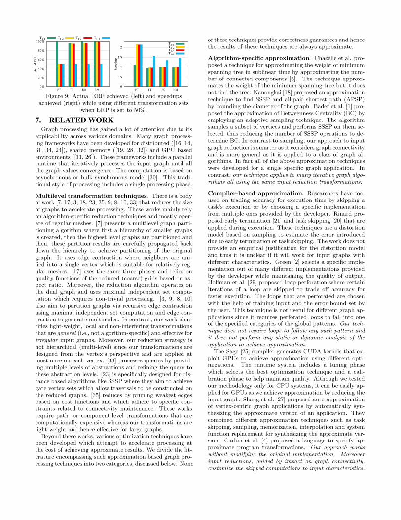
ated using different transformation sets T1−k (1 ≥ k ≤ 4).To clearly present the impact of transformations on both,the size of reduced graphs and the savings in execution time,we select ERP = 50% and only consider the SSSP bench-mark. Figure 9 shows the speedups achieved for each of thegraphs transformed using the transformation sets, comparedto the Baseline. Since the transformations being appliedhave their pre-conditions which need to be satisfied, the ac-tual ERP using a smaller transformation set can be higherthan the requested ERP of 50%. Hence, we also present theactual ERP obtained using the transformation sets.

As we can see in Figure 9, T1, T2 and T3 collectively reduceonly small portion of TT, UK and RM graphs; T1−3 achieves95.26%, 96.58% and 99.39% ERP for TT, UK and RM re-spectively. Due to this, little to no savings are achieveduntil T4 is included in the transformation sets for whichspeedups of up to 1.34-1.55× are achieved. FT graph, onthe other hand, is amenable to T2 and T3, allowing 50% ERPto be achieved for T1−2 and T1−3 too. Hence, the speedupsachieved for those transformation sets are ∼2.15×.

0%

20%

40%

60%

80%

100%

FT TT UK RM

Actu

al ER

PΤ1-1 Τ1-2 Τ1-3 Τ1-4

0

0.5

1

1.5

2

FT TT UK RM

Spee

dup

Τ1-1Τ1-2Τ1-3Τ1-4

Figure 9: Actual ERP achieved (left) and speedupsachieved (right) while using different transformation sets

when ERP is set to 50%.

7. RELATED WORKGraph processing has gained a lot of attention due to its

applicability across various domains. Many graph process-ing frameworks have been developed for distributed ([16, 14,31, 34, 24]), shared memory ([19, 28, 32]) and GPU basedenvironments ([11, 26]). These frameworks include a parallelruntime that iteratively processes the input graph until allthe graph values convergence. The computation is based onasynchronous or bulk synchronous model [30]. This tradi-tional style of processing includes a single processing phase.

Multilevel transformation techniques. There is a bodyof work [7, 17, 3, 18, 23, 35, 9, 8, 10, 33] that reduces the sizeof graphs to accelerate processing. These works mainly relyon algorithm-specific reduction techniques and mostly oper-ate of regular meshes. [7] presents a multilevel graph parti-tioning algorithm where first a hierarchy of smaller graphsis created, then the highest level graphs are partitioned andthen, these partition results are carefully propagated backdown the hierarchy to achieve partitioning of the originalgraph. It uses edge contraction where neighbors are uni-fied into a single vertex which is suitable for relatively reg-ular meshes. [17] uses the same three phases and relies onquality functions of the reduced (coarse) grids based on as-pect ratio. Moreover, the reduction algorithm operates onthe dual graph and uses maximal independent set compu-tation which requires non-trivial processing. [3, 9, 8, 10]also aim to partition graphs via recursive edge contractionusing maximal independent set computation and edge con-traction to generate multinodes. In contrast, our work iden-tifies light-weight, local and non-interfering transformationsthat are general (i.e., not algorithm-specific) and effective forirregular input graphs. Moreover, our reduction strategy isnot hierarchical (multi-level) since our transformations aredesigned from the vertex’s perspective and are applied atmost once on each vertex. [33] processes queries by provid-ing multiple levels of abstractions and refining the query tothese abstraction levels. [23] is specifically designed for dis-tance based algorithms like SSSP where they aim to achievegate vertex sets which allow traversals to be constructed onthe reduced graphs. [35] reduces by pruning weakest edgesbased on cost functions and which adhere to specific con-straints related to connectivity maintenance. These worksrequire path- or component-level transformations that arecomputationally expensive whereas our transformations arelight-weight and hence effective for large graphs.

Beyond these works, various optimization techniques havebeen developed which attempt to accelerate processing atthe cost of achieving approximate results. We divide the lit-erature encompassing such approximation based graph pro-cessing techniques into two categories, discussed below. None

of these techniques provide correctness guarantees and hencethe results of these techniques are always approximate.

Algorithm-specific approximation. Chazelle et al. pro-posed a technique for approximating the weight of minimumspanning tree in sublinear time by approximating the num-ber of connected components [5]. The technique approxi-mates the weight of the minimum spanning tree but it doesnot find the tree. Nanongkai [18] proposed an approximationtechnique to find SSSP and all-pair shortest path (APSP)by bounding the diameter of the graph. Bader et al. [1] pro-posed the approximation of Betweenness Centrality (BC) byemploying an adaptive sampling technique. The algorithmsamples a subset of vertices and performs SSSP on them se-lected, thus reducing the number of SSSP operations to de-termine BC. In contrast to sampling, our approach to inputgraph reduction is smarter as it considers graph connectivityand is more general as it is applied to a class of graph al-gorithms. In fact all of the above approximation techniqueswere developed for a single specific graph application. Incontrast, our technique applies to many iterative graph algo-rithms all using the same input reduction transformations.

Compiler-based approximation. Researchers have foc-used on trading accuracy for execution time by skipping atask’s execution or by choosing a specific implementationfrom multiple ones provided by the developer. Rinard pro-posed early termination [21] and task skipping [20] that areapplied during execution. These techniques use a distortionmodel based on sampling to estimate the error introduceddue to early termination or task skipping. The work does notprovide an empirical justification for the distortion modeland thus it is unclear if it will work for input graphs withdifferent characteristics. Green [2] selects a specific imple-mentation out of many different implementations providedby the developer while maintaining the quality of output.Hoffman et al. [29] proposed loop perforation where certainiterations of a loop are skipped to trade off accuracy forfaster execution. The loops that are perforated are chosenwith the help of training input and the error bound set bythe user. This technique is not useful for different graph ap-plications since it requires perforated loops to fall into oneof the specified categories of the global patterns. Our tech-nique does not require loops to follow any such pattern andit does not perform any static or dynamic analysis of theapplication to achieve approximation.

The Sage [25] compiler generates CUDA kernels that ex-ploit GPUs to achieve approximation using different opti-mizations. The runtime system includes a tuning phasewhich selects the best optimization technique and a cali-bration phase to help maintain quality. Although we testedour methodology only for CPU systems, it can be easily ap-plied for GPUs as we achieve approximation by reducing theinput graph. Shang et al. [27] proposed auto-approximationof vertex-centric graph applications by automatically syn-thesizing the approximate version of an application. Theycombined different approximation techniques such as taskskipping, sampling, memorization, interpolation and systemfunction replacement for synthesizing the approximate ver-sion. Carbin et al. [4] proposed a language to specify ap-proximate program transformations. Our approach workswithout modifying the original implementation. Moreoverinput reductions, guided by impact on graph connectivity,customize the skipped computations to input characteristics.

8. CONCLUSIONWe proposed input reduction transformations and faster

iterative graph algorithms that run in two phases: first, us-ing the reduced input graph, and second using the originalgraph along with the results from first phase. We evaluatedour two-phased model using Galois; our experiments withmultiple algorithms and large graphs show that our tech-nique reduces execution time by 1.25× to 2.14×.

AcknowledgmentsThe authors thank their shepherd, Shuaiwen Song, for hisguidance in preparing the final version of this paper, as wellas the anonymous reviewers for their feedback and sugges-tions. This work is supported by NSF grants CCF-1524852and CCF-1318103 to the University of California Riverside.

9. REFERENCES[1] D. A. Bader, S. Kintali, K. Madduri, and M. Mihail.

Approximating Betweenness Centrality. WAW, 2007.[2] W. Baek and T. M. Chilimbi. Green: A Framework

for Supporting Energy-Conscious Programming usingControlled Approximation. PLDI, pages 198-209, 2010.

[3] S. T. Barnard and H. D. Simon. Fast MultilevelImplementation of Recursive Spectral Bisection forPartitioning Unstructured Problems. Concurrency:Practice and experience, 6(2):101–117, 1994.

[4] M. Carbin, D. Kim, S. Misailovic, and M. C. Rinard.Proving Acceptability Properties of RelaxedNondeterministic Approximate Programs. PLDI 2013.

[5] B. Chazelle, R. Rubinfeld, and L. Trevisan.Approximating the Minimum Spanning Tree Weightin Sublinear Time. International Colloquium onAutomata, Languages and Programming, 2005.

[6] A. Farahat, T. LoFaro, J. C. Miller, G. Rae, and L. A.Ward. Authority Rankings from HITS, Pagerank, andSALSA: Existence, Uniqueness, and Effect ofInitialization. SIAM J. Scientific Computing,27(4):1181–1201, 2005.

[7] B. Hendrickson and R. Leland. A MultilevelAlgorithm for Partitioning Graphs. ACM/IEEEConference on Supercomputing, 1995.

[8] G. Karypis and V. Kumar. Multilevel GraphPartitioning Schemes. ICPP (3), pages 113–122, 1995.

[9] G. Karypis and V. Kumar. A Fast and High QualityMultilevel Scheme for Partitioning Irregular Graphs.SIAM J. Sci. Comput., 20(1):359–392, Dec. 1998.

[10] G. Karypis and V. Kumar. Multilevel K-wayPartitioning Scheme for Irregular Graphs. JPDC,48(1):96–129, 1998.

[11] F. Khorasani, R. Gupta, and L. N. Bhuyan. ScalableSIMD-Efficient Graph Processing on GPUs. PACT’15.

[12] J. Kunegis. KONECT: The Koblenz NetworkCollection. WWW Companion, pages 1343-1350, 2013.

[13] A. Kyrola, G. Blelloch, and C. Guestrin. GraphChi:Large-scale Graph Computation on Just a PC. OSDI,pages 31-46, 2012.

[14] Y. Low, D. Bickson, J. Gonzalez, C. Guestrin,A. Kyrola, and J. M. Hellerstein. DistributedGraphLab: A Framework for Machine Learning andData Mining in the Cloud. VLDB Endowment, 2012.

[15] Y. Low, J. E. Gonzalez, A. Kyrola, D. Bickson, C. E.Guestrin, and J. Hellerstein. GraphLab: A NewFramework for Parallel Machine Learning. arXivpreprint arXiv:1408.2041, 2014.

[16] G. Malewicz, M. H. Austern, A. J. Bik, J. C. Dehnert,I. Horn, N. Leiser, and G. Czajkowski. Pregel: ASystem for Large-scale Graph Processing. SIGMODInternational Conf. on Management of Data, 2010.

[17] I. Moulitsas and G. Karypis. Multilevel Algorithms forGenerating Coarse Grids for Multigrid Methods.Supercomputing, pages 45–45, 2001.

[18] D. Nanongkai. Distributed Approximation Algorithmsfor Weighted Shortest Paths. STOC, pages 565-573,2014.

[19] K. Pingali, D. Nguyen, M. Kulkarni, M. Burtscher,M. A. Hassaan, R. Kaleem, T.-H. Lee, A. Lenharth,R. Manevich, M. Mendez-Lojo, D. Prountzos, andX. Sui. The Tao of Parallelism in Algorithms. PLDI,pages 12-25, 2011.

[20] M. Rinard. Probabilistic Accuracy Bounds forFault-tolerant Computations that Discard Tasks. ICS,pages 324-334, 2006.

[21] M. C. Rinard. Using Early Phase Termination toEliminate Load Imbalances at Barrier SynchronizationPoints. OOPSLA, pages 369-386, 2007.

[22] A. Roy, I. Mihailovic, and W. Zwaenepoel. X-stream:Edge-centric Graph Processing using StreamingPartitions. SOSP, pages 472–488, 2013.

[23] N. Ruan, R. Jin, and Y. Huang. Distance PreservingGraph Simplification. ICDM, pages 1200–1205, 2011.

[24] S. Salihoglu and J. Widom. GPS: A Graph ProcessingSystem. SSDBM, pages 22:1-22:12, 2013.

[25] M. Samadi, J. Lee, D. A. Jamshidi, A. Hormati, andS. Mahlke. SAGE: Self-tuning Approximation forGraphics Engines. MICRO-46, pages 13-24, 2013.

[26] D. Sengupta, S. L. Song, K. Agarwal and K. Schwan.GraphReduce: Processing Large-scale Graphs onAccelerator-based Systems. SC, pages 28:1–12, 2015.

[27] Z. Shang and J. X. Yu. Auto-approximation of GraphComputing. VLDB Endow., pages 1833-1844, 2014.

[28] J. Shun and G. E. Blelloch. Ligra: A LightweightGraph Processing Framework for Shared Memory.PPoPP, pages 135-146, 2013.

[29] S. Sidiroglou-Douskos, S. Misailovic, H. Hoffmann,and M. Rinard. Managing Performance vs. AccuracyTrade-offs with Loop Perforation. ESEC/FSE 2011.

[30] L. G. Valiant. A Bridging Model for ParallelComputation. CACM, 33(8):103–111, 1990.

[31] K. Vora, S. C. Koduru, and R. Gupta. ASPIRE:Exploiting Asynchronous Parallelism in IterativeAlgorithms using a Relaxed Consistency Based DSM.OOPSLA, pages 861-878, 2014.

[32] G. Wang, W. Xie, A. J. Demers, and J. Gehrke.Asynchronous Large-scale Graph Processing MadeEasy. CIDR 2013.

[33] K. Wang, G. Xu, Z. Su and Y. D. Liu. GraphQ:Graph Query Processing with AbstractionRefinement—Scalable and Programmable Analyticsover Very Large Graphs on a Single PC. USENIXATC, pages 387–401, 2015.

[34] R. S. Xin, J. E. Gonzalez, M. J. Franklin, andI. Stoica. GraphX: A Resilient Distributed GraphSystem on Spark. International Workshop on GraphData Management Experiences and Systems, 2013.

[35] F. Zhou, S. Malher, and H. Toivonen. NetworkSimplification with Minimal Loss of Connectivity.ICDM, pages 659–668, 2010.

efﬁcient processing of large graphs via input...

Documents