efﬁcient surface reconstruction using generalized...

Efficient Surface Reconstruction using Generalized

Coulomb Potentials

Andrei C. Jalba and Jos B. T. M. Roerdink Senior Member, IEEE

Abstract—We propose a novel, geometrically adaptive method for surface reconstruction from noisy and sparse point clouds, withoutorientation information. The method employs a fast convection algorithm to attract the evolving surface towards the data points. Theforce field in which the surface is convected is based on generalized Coulomb potentials evaluated on an adaptive grid (i.e., an octree)using a fast, hierarchical algorithm. Formulating reconstruction as a convection problem in a velocity field generated by Coulombpotentials offers a number of advantages. Unlike methods which compute the distance from the data set to the implicit surface, whichare sensitive to noise due to the very reliance on the distance transform, our method is highly resilient to shot noise since global,generalized Coulomb potentials can be used to disregard the presence of outliers due to noise. Coulomb potentials represent long-range interactions that consider all data points at once, and thus they convey global information which is crucial in the fitting process.Both the spatial and temporal complexities of our spatially-adaptive method are proportional to the size of the reconstructed object,which makes our method compare favorably with respect to previous approaches in terms of speed and flexibility. Experiments withsparse as well as noisy data sets show that the method is capable of delivering crisp and detailed yet smooth surfaces.

Index Terms—Surface reconstruction, Implicit surfaces, Octrees, Generalized Coulomb potentials, Polygonization.

1 INTRODUCTION

Surface reconstruction is challenging because the topology of the realsurface is unknown, acquired data can be non-uniform and contami-nated by noise, and reconstructing surfaces from large data sets can beprohibitively expensive in terms of computations or memory usage. Alack of information about the surface orientation at the acquired sam-ples may further complicate the problem.

We propose a novel, geometrically adaptive method for surfacereconstruction without using orientation information. It employs afast convection algorithm (inspired by the tagging method of Zhao etal. [31]) to attract the evolving surface (i.e., the current approximationto the final surface) towards the data points. The force field in whichthe surface is convected is based on generalized Coulomb potentialsevaluated on an adaptive grid (i.e., an octree) using the fast, hierarchi-cal algorithm of Barnes and Hut [6]. The potentials are used to attractthe evolving surface towards the data points and to remove outliers dueto noise. When the convection process ends, the characteristic func-tion χ (defined as 1 at points inside the object, and 0 at points outside)yields the final implicit surface, which is polygonized using a meshingalgorithm based on tetrahedral subdivision of octree cells [27].

Formulating surface reconstruction as a convection problem offers anumber of advantages. Most methods for implicit surface fitting com-pute a signed distance function from the given point data and representthe reconstructed surface as an iso-contour of this function. However,these approaches are very sensitive to outliers (shot noise) due to thevery reliance on the distance transform. By contrast, global gener-alized Coulomb potentials can be used to disregard the presence ofoutliers due to noise. Some methods first locally fit the data and thencombine these approximations by blending the locally fitting (basis)functions. Unlike this, Coulomb potentials represent long-range inter-actions for all data points at once, and thus convey global information.As computing Coulomb potentials is of paramount importance in abroad variety of problems, we can rely on a very efficient method forcomputing Coulomb potentials, to arrive at reconstruction with scal-able computational time and memory requirements.

Both authors are with the Institute for Mathematics and Computing

Science, University of Groningen, The Netherlands.

E-mail: [email protected], [email protected].

Manuscript received 31 March 2007; accepted 1 August 2007; posted online

27 October 2007.

For information on obtaining reprints of this article, please send e-mail to:

[email protected].

The main contributions of this paper include:

• An improved geometrically-adaptive method for surface recon-struction based on an implicit surface representation which onlyrequires information about the position of the samples and is ro-bust to the presence of noise and missing data.

• A hierarchical and adaptive representation based on octrees,which allows scalable reconstruction at different levels of detail.

• New algorithms for surface reconstruction based on convectionof surfaces in generalized Coulomb potentials.

2 RELATED WORK

Popular explicit surface representations are based on parametric (e.g.,NURBS, B-spline and Bezier patches) and triangulated surfaces. Ma-jor drawbacks of parametric representations are that patches shouldbe combined to form closed surfaces, which can be very difficult forarbitrary data sets, and noisy data sets are difficult to deal with. Tri-angulated surfaces are usually based on tools from computational ge-ometry, such as Delaunay triangulations and their duals, Voronoi dia-grams. Most methods in this class extract subsets of faces of Delaunaytriangulations to yield the reconstructed surface [3, 4, 15]. They ex-actly interpolate the data, and therefore, are rather sensitive to noise.Moreover, inserting hundreds of thousands of points into a triangula-tion is computationally expensive. Examples are Alpha Shapes [15],the (Power) Crust algorithm [3,4], and the Ball-Pivoting algorithm [7].Recently, Giesen and John [16] introduced the notion of flow in com-putational geometry, and Scheidegger et al. [28] proposed an adaptivemethod based on the Moving Least-Squares algorithm.

Much research is devoted to efficient reconstruction methods re-lying on implicit surface representations, as these offer a number ofadvantages. Compared to explicit methods, implicit ones elegantlydeal with objects of arbitrary topology, blend and perform Booleanoperations on surface primitives, and fill holes automatically. The tra-ditional approach is to compute a signed distance function and repre-sent the reconstructed implicit surface by an iso-contour of this func-tion [5,8,12,17]. This requires a way to distinguish between the insideand outside of closed surfaces. E.g., Hoppe et al. [17] approximate thenormal at each data point by fitting a tangent plane in its neighbor-hood, using principal component analysis. Zhao et al. [31] use thelevel-set formalism [26] for noise-free surface reconstruction. Theirmethod handles complicated topology and deformations, and the re-constructed surface is smoother than piecewise linear. The main draw-back is the sensitivity to shot noise, due to reliance on the distance

Published 14 September 2007.

1512

1077-2626/07/$25.00 © 2007 IEEE Published by the IEEE Computer Society

IEEE TRANSACTIONS ON VISUALIZATION AND COMPUTER GRAPHICS, VOL. 13, NO. 6, NOVEMBER/DECEMBER 2007

Authorized licensed use limited to: IEEE Xplore. Downloaded on October 19, 2008 at 00:37 from IEEE Xplore. Restrictions apply.

transform. The work of Zhao et al. [31] inspired researchers fromthe computational-geometry community to develop ’geometric con-vection’ algorithms [2, 11] in the context of surface reconstruction.These methods deform a closed oriented pseudo-surface embedded inthe 3D Delaunay triangulation of the sampled points, and yield the re-constructed surface as a set of oriented facets of the triangulation. Al-though these methods tolerate small amounts of Gaussian noise, theyare computationally expensive.

More recently, blending globally or locally supported implicit prim-itives (e.g. Radial Basis Functions or RBFs) became the favorite tech-nique [10, 13, 21, 23]. Turk and O’Brien [30] and Carr et al. [10]use globally supported RBFs by solving a large and dense linear sys-tem of equations. Since the ideal RBFs are globally-supported andnon-decaying, the solution matrix is dense and ill-conditioned [20].Moreover, these methods are very sensitive to noise because localchanges of the positions of the input points have global effects on thereconstructed surface. Morse et al. [23] and Ohtake et al. [25] usecompactly-supported RBFs to achieve local control and reduce com-putational costs by solving a sparse linear system. Dinh et al. [13]use RBFs and volumetric regularization to handle noisy and sparserange data sets. Recently, Ohtake et al. [24] proposed the so-called’partition of the unity implicits’, which can be regarded as the combi-nation of algebraic patches and RBFs. Carr et al. [9] further addresssurface reconstruction from noisy range data by fitting a RBF to thedata and convolving with a smoothing kernel during the evaluationof the RBF. Kojekine et al. [21] use compactly-supported RBFs andan octree data structure such that the resulting matrix of the systemis band-diagonal, thus reducing computational costs. More recently,Kazhdan [19] proposed to use the Fourier transform for computingthe characteristic function of the solid model, and then standard iso-surfacing techniques (i.e., marching cubes) to triangulate its boundary.Although (small) displacements of the positions and normals of thesamples are handled well, the temporal and spatial complexities are cu-bic in the (uniform) grid resolution. An improved, geometrically adap-tive method [20] with quadratic complexities, formulates reconstruc-tion as a Poisson problem which is then tackled using efficient Poissonsolvers. However, both methods assume that orientation informationis available. Kolluri et al. [22] introduce a noise-resistant algorithm forwatertight reconstruction based on spectral graph partitioning. Sincethe local spectral partitioner uses a global view of the model, their al-gorithm can ignore outliers and patch holes in under-sampled regions.The method is computationally expensive as it solves an eigenvalueproblem on a large graph formed by a subset of the Voronoi verticesof the input set. Tang and Medioni [29] use tensor-voting to developa method which is resilient to noise and copes well with sparse data.The downside of this method is its cubic spatio-temporal complexities.In [18] regularized membrane potentials are used to aggregate the in-put points on a uniform grid, then a labeling algorithm similar to thatin [31] is used to define an implicit surface, which is smoothed usinga mass-spring system and as a final step polygonized. However, thismethod has cubic complexities similar to the FFT method in [19].

Similarly to RBF approaches and Poisson reconstruction, ourmethod creates smooth surfaces that approximate noisy data, andcombines some positive aspects of both global and local approxima-tion schemes. Convection is performed in a global field (Coulombforce field) which does not rely on computing local neighborhoods forblending. However, after the indicator function of the solid has beencomputed, we do employ blending based on compactly-supported ker-nels to produce smooth triangulated surfaces.

3 THE PROPOSED METHOD

Let S denote an input data set of samples (points, lines, etc.) lyingon or near the surface ∂MMM of an unknown object M. The problemis to accurately reconstruct the indicator function χ of M, and thento approximate the surface ∂MMM by a watertight, smooth triangulatediso-surface.

Given a flexible, arbitrary enclosing surface ΓΓΓ, the reconstructionproblem is formulated as the convection of ΓΓΓ in a conservative velocityfield vvv = −∇φ created by the input data points, as described by the

differential equation

dΓΓΓ

dt= vvv(ΓΓΓ(t)) = −∇φ (ΓΓΓ(t)) . (1)

We assume that φ is the electric scalar potential (Coulomb potential),such that the velocity field becomes the electric field vvv = EEE ≡ −∇φ .We regard the sample points si, si ∈ S, as electric charges qi with posi-tion vectors rrri, i = 1,2, . . .N generating a charge distribution ρ . Hencewe can solve for φ by numerically approximating Poisson’s equation

∇2φ = −ρ

ε0. (2)

Solving for Poisson’s equation in this case has the problem that thelong-range nature of Coulomb interactions is not properly taken intoaccount. Moreover, Poisson’s equation requires a continuous chargedistribution and not a set of discrete charges, which are in fact justa set of singularities. This problem has been addressed in [20] byconvolving the input points with a Gaussian kernel prior to solvingPoisson’s equation. Additionally, in [20] the authors directly solvea Poisson equation for the characteristic function, assuming howeverthat the orientation of the sample points is available. Discretizing thesuperposition integral, the potential φ is a sum of potentials generatedby each charge taken in isolation. However, this potential is inade-quate for our purposes (see Fig. 2). Therefore, we use higher ordergeneralized Coulomb potentials which decay faster with distance thanas inverse of distance, i.e.,

φ(rrri) = ∑j �=i

q j

|rrri − rrr j|m, (3)

where m > 1 and we removed the constants appearing in the physi-cal formulation. Note that similar potentials have been successfullyused for computing medial axes of 3D shapes [1]. In our case a high-order potential should be used for noise-free data when an accuratereconstruction is desired. By contrast, we show that for noisy data asmaller-order potential can be used to detect and remove outlier data.

During convection generalized Coulomb potentials have to be eval-uated not only at the sample positions, but at all centers of the (adap-tive) grid cells. This is required by the fast convection algorithm (de-scribed in Section 4.3) which, starting from the bounding box of thegrid, follows increasing paths of the scalar field until regional max-ima (corresponding to the sample points) and ridges are reached. As itsweeps the volume, this algorithm labels grid cells as exterior, so thatafter propagation the remaining cells qualify as interior to the surface.Naive evaluations of these potentials at all grid positions is expensivefor large grid resolutions. So we need to use fast adaptive solvers (seeSection 4.2) to approximate them.

Having labeled the cells of the adaptive grid (octree) as exterior andinterior to the surface, and thus equivalently determined χ , we com-pute a smoothed version χ of χ as the weighted sum of contributionsof nearby cells (estimated during polygonization). The weights are ob-tained by evaluating the quadratic (approximating) C1–continuous B-spline of Dodgson [14]. This has second order interpolation error, andsince it evaluates to zero and has vanishing derivatives at the bound-ary it is conducive to stability. Moreover, it is inexpensive to computesince it requires only three multiplications and three additions for eachevaluation.

4 IMPLEMENTATION

4.1 Adaptive octree-based approximation

Discretizing the problem on a regular 3D grid is impractical since thememory for maintaining such a uniform structure becomes prohibitivefor fine-grain reconstruction. However, since accurate representationsare only required close to the data set, we can use an adaptive gridbased on an octree to efficiently evaluate Coulomb potentials and torepresent and triangulate the implicit function.

Given samples si ∈ S, i = 1,2, . . . ,N regarded as particles with posi-tion si.p and charge si.q, and a maximum tree depth D, the octree O is

1513IEEE TRANSACTIONS ON VISUALIZATION AND COMPUTER GRAPHICS, VOL. 13, NO. 6, NOVEMBER/DECEMBER 2007


built by calling the function octInsert shown in Algorithm 1 for eachparticle, with n set to the root node r. When the maximum tree depthD is reached for a non-empty leaf l, l ∈ O, the node is not further sub-divided if a new particle is to be assigned to it. Instead, the centroidand total charge of the subset Z of all particles sk that would have beenassigned to the subtree rooted at l in an infinitely-deep octree are com-puted and stored in a new particle ss that is assigned to l. All particlessk can now be discarded, as they are no longer needed. Effectivelywe implement a low-pass filter acting on particle positions, since thegiven (maximum) resolution (1/2D) cannot be exceeded anyway, i.e.,

ss.p ←∑sk∈Z sk.q sk.p

∑sk∈Z sk.q, ss.q ← ∑

sk∈Z

sk.q (4)

When initially all particles have the same charge (we use q = 1), thetotal charge of such particles will be larger than that of usual particlesassigned to non-empty leaves.

Algorithm 1 Insert particle si in the subtree rooted at n.

function octInsert(si, n)

if subtree rooted at n contains more than one particle thendetermine child c of n which contains particle si;octInsert(si, c);

else if subtree rooted at n contains exactly one particle thenif n.depth ≥ D then

determine particle s j contained in n;create new particle ss with charge ss.q = si.q+ s j.q

and position ss.p = (si.q · si.p+ s j.q · s j.p)/ss.q;assign ss to n and discard particles si and s j;

elseadd n’s eight children to the octree;move particle s j already in n into the child in which it lies;let c be the child in which si lies;octInsert(si, c);

elsestore si at node n;

After octree construction the octree is balanced (by subdividingnodes until any two neighboring cells differ at most by one in depth),as required by both the meshing (see Section 4.4) and convection al-gorithms (see Section 4.3 and Fig. 2).

4.2 Fast evaluation of the Coulomb potentials

To evaluate the generalized Coulomb potentials within any desiredprecision on the adaptive grid obtained by stacking the cells of thebalanced octree, we rely on the fast, hierarchical algorithm of Barnesand Hut [6], thus trading accuracy for speed. The Barnes-Hut algo-rithm can be summarized as follows: (i) construct an octree whereeach leaf contains at most one particle, (ii) for each octree cell, com-pute the centroid and total charge for the particles it contains, (iii) tra-verse the tree to evaluate the potential at any desired grid location. Thefirst step is accomplished using the function octInsert in Algorithm 1.The second step is implemented in a depth-first-search traversal of thebalanced tree Ob, in which the total charge n.q and the centroid n.cof each node n ∈ Ob are computed (using Eq. (4)) and stored at eachnode.

Then we come to the core of the Barnes-Hut algorithm, evaluatingthe potential at an arbitrary location ppp. A small positive test charge qt

(with value qt = 1) is placed at position ppp, i.e.,

φ(ppp) = qt

N

∑i=1

qi

|rrri − ppp|m. (5)

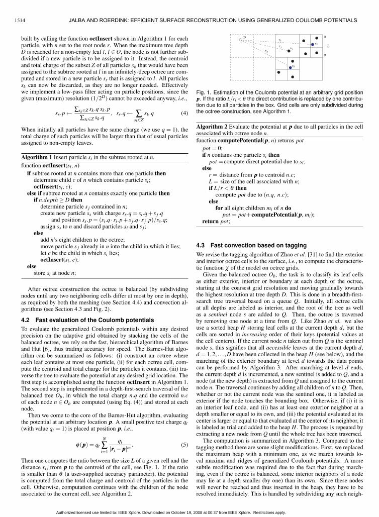
Then one computes the ratio between the size L of a given cell and thedistance ri, from ppp to the centroid of the cell, see Fig. 1. If the ratiois smaller than θ (a user-supplied accuracy parameter), the potentialis computed from the total charge and centroid of the particles in thecell. Otherwise, computation continues with the children of the nodeassociated to the current cell, see Algorithm 2.

L

ri

rj

rk

si

sj

sk

p

Fig. 1. Estimation of the Coulomb potential at an arbitrary grid positionppp. If the ratio L/ri < θ the direct contribution is replaced by one contribu-tion due to all particles in the box. Grid cells are only subdivided duringthe octree construction, see Algorithm 1.

Algorithm 2 Evaluate the potential at ppp due to all particles in the cellassociated with octree node n.

function computePotential(ppp, n) returns pot

pot = 0;if n contains one particle si then

pot =compute direct potential due to si;else

r = distance from ppp to centroid n.c;L = size of the cell associated with n;if L/r < θ then

compute pot due to (n.q, n.c);else

for all eight children mi of n dopot = pot+computePotential(ppp, mi);

return pot;

4.3 Fast convection based on tagging

We revise the tagging algorithm of Zhao et al. [31] to find the exteriorand interior octree cells to the surface, i.e., to compute the characteris-tic function χ of the model on octree grids.

Given the balanced octree Ob, the task is to classify its leaf cellsas either exterior, interior or boundary at each depth of the octree,starting at the coarsest grid resolution and moving gradually towardsthe highest resolution at tree depth D. This is done in a breadth-first-search tree traversal based on a queue Q. Initially, all octree cellsat all depths are labeled as interior, and the root of the tree as wellas a sentinel node s are added to Q. Then, the octree is traversedby removing one node at a time from Q. Like Zhao et al. we alsouse a sorted heap H storing leaf cells at the current depth d, but thecells are sorted in increasing order of their keys (potential values atthe cell centers). If the current node n taken out from Q is the sentinelnode s, this signifies that all accessible leaves at the current depth d,d = 1,2, . . . ,D have been collected in the heap H (see below), and themarching of the exterior boundary at level d towards the data pointscan be performed by Algorithm 3. After marching at level d ends,the current depth d is incremented, a new sentinel is added to Q, and anode (at the new depth) is extracted from Q and assigned to the currentnode n. The traversal continues by adding all children of n to Q. Then,whether or not the current node was the sentinel one, it is labeled asexterior if the node touches the bounding box. Otherwise, if (i) it isan interior leaf node, and (ii) has at least one exterior neighbor at adepth smaller or equal to its own, and (iii) the potential evaluated at itscenter is larger or equal to that evaluated at the center of its neighbor, itis labeled as trial and added to the heap H. The process is repeated byextracting a new node from Q until the whole tree has been traversed.

The computation is summarized in Algorithm 3. Compared to thetagging method there are some slight modifications. First, we replacedthe maximum heap with a minimum one, as we march towards lo-cal maxima and ridges of generalized Coulomb potentials. A moresubtle modification was required due to the fact that during march-ing, even if the octree is balanced, some interior neighbors of a nodemay lie at a depth smaller (by one) than its own. Since these nodeswill never be reached and thus inserted in the heap, they have to beresolved immediately. This is handled by subdividing any such neigh-

1514 JALBA AND ROERDINK: EFFICIENT SURFACE RECONSTRUCTION USING GENERALIZED COULOMB POTENTIALS


Algorithm 3 Label cells as exterior or boundary.

function marchExterior(H)

while not empty heap H doextract node n from H;pn = computePotential(n.ccceeennnttteeerrr, root);for each leaf m, neighbor of n, m.depth ≤ n.depth do

if m is interior and m.depth < n.depth thensubdivide m;find neighbor k of n among the children of m;assign m = k and continue;

if m is interior thenpm = computePotential(mmm...ccceeennnttteeerrr, root);if pm + ε < pn then

label n as boundary;continue with extracting a new node from H;

label n as exterior;for each leaf m, neighbor of n do

if m is interior thenlabel m as trial;insert m onto H;

bor and continuing the marching process normally. Additionally, auser-specified parameter ε has been introduced to allow the marchingprocess to continue if the potential at a neighboring node is not smallenough compared to that of the current node. For noise-free data setswe set this parameter to ε = 0, whereas for data sets corrupted by out-liers we allow for some variation and set ε to a value larger than zero(see Section 5.5).

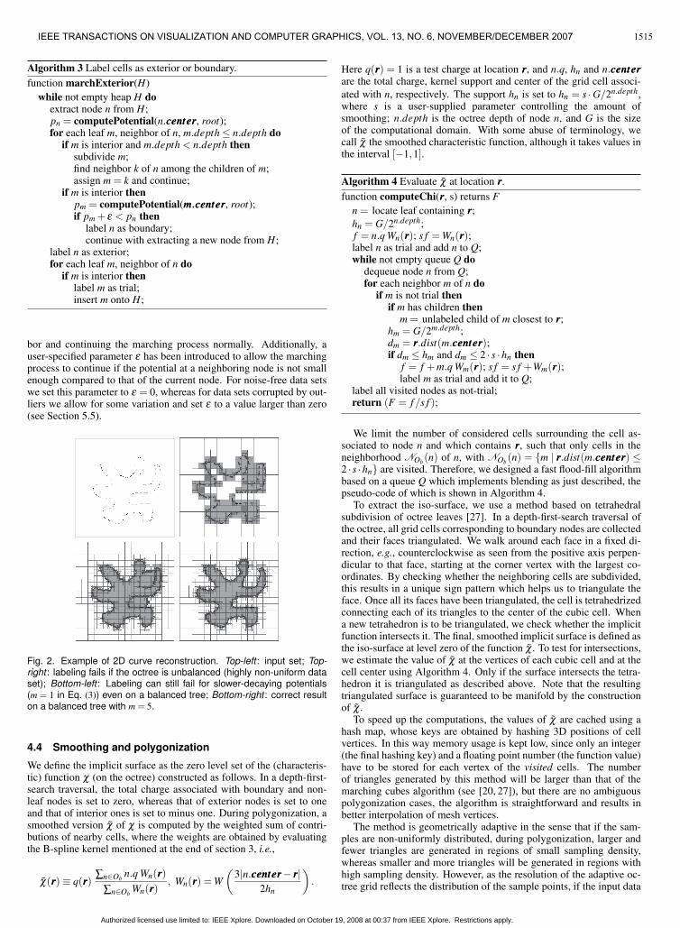
Fig. 2. Example of 2D curve reconstruction. Top-left : input set; Top-right : labeling fails if the octree is unbalanced (highly non-uniform dataset); Bottom-left : Labeling can still fail for slower-decaying potentials(m = 1 in Eq. (3)) even on a balanced tree; Bottom-right : correct resulton a balanced tree with m = 5.

4.4 Smoothing and polygonization

We define the implicit surface as the zero level set of the (characteris-tic) function χ (on the octree) constructed as follows. In a depth-first-search traversal, the total charge associated with boundary and non-leaf nodes is set to zero, whereas that of exterior nodes is set to oneand that of interior ones is set to minus one. During polygonization, asmoothed version χ of χ is computed by the weighted sum of contri-butions of nearby cells, where the weights are obtained by evaluatingthe B-spline kernel mentioned at the end of section 3, i.e.,

χ(rrr) ≡ q(rrr)∑n∈Ob

n.q Wn(rrr)

∑n∈ObWn(rrr)

, Wn(rrr) = W

(3|n.ccceeennnttteeerrr− rrr|

2hn

).

Here q(rrr) = 1 is a test charge at location rrr, and n.q, hn and n.ccceeennnttteeerrrare the total charge, kernel support and center of the grid cell associ-

ated with n, respectively. The support hn is set to hn = s ·G/2n.depth,where s is a user-supplied parameter controlling the amount ofsmoothing; n.depth is the octree depth of node n, and G is the sizeof the computational domain. With some abuse of terminology, wecall χ the smoothed characteristic function, although it takes values inthe interval [−1,1].

Algorithm 4 Evaluate χ at location rrr.

function computeChi(rrr, s) returns F

n = locate leaf containing rrr;

hn = G/2n.depth;f = n.q Wn(rrr); s f = Wn(rrr);label n as trial and add n to Q;while not empty queue Q do

dequeue node n from Q;for each neighbor m of n do

if m is not trial thenif m has children then

m = unlabeled child of m closest to rrr;hm = G/2m.depth;dm = rrr.dist(m.ccceeennnttteeerrr);if dm ≤ hm and dm ≤ 2 · s ·hn then

f = f +m.q Wm(rrr); s f = s f +Wm(rrr);label m as trial and add it to Q;

label all visited nodes as not-trial;return (F = f /s f );

We limit the number of considered cells surrounding the cell as-sociated to node n and which contains rrr, such that only cells in theneighborhood NOb

(n) of n, with NOb(n) = {m | rrr.dist(m.ccceeennnttteeerrr) ≤

2 · s ·hn} are visited. Therefore, we designed a fast flood-fill algorithmbased on a queue Q which implements blending as just described, thepseudo-code of which is shown in Algorithm 4.

To extract the iso-surface, we use a method based on tetrahedralsubdivision of octree leaves [27]. In a depth-first-search traversal ofthe octree, all grid cells corresponding to boundary nodes are collectedand their faces triangulated. We walk around each face in a fixed di-rection, e.g., counterclockwise as seen from the positive axis perpen-dicular to that face, starting at the corner vertex with the largest co-ordinates. By checking whether the neighboring cells are subdivided,this results in a unique sign pattern which helps us to triangulate theface. Once all its faces have been triangulated, the cell is tetrahedrizedconnecting each of its triangles to the center of the cubic cell. Whena new tetrahedron is to be triangulated, we check whether the implicitfunction intersects it. The final, smoothed implicit surface is defined asthe iso-surface at level zero of the function χ . To test for intersections,we estimate the value of χ at the vertices of each cubic cell and at thecell center using Algorithm 4. Only if the surface intersects the tetra-hedron it is triangulated as described above. Note that the resultingtriangulated surface is guaranteed to be manifold by the constructionof χ .

To speed up the computations, the values of χ are cached using ahash map, whose keys are obtained by hashing 3D positions of cellvertices. In this way memory usage is kept low, since only an integer(the final hashing key) and a floating point number (the function value)have to be stored for each vertex of the visited cells. The numberof triangles generated by this method will be larger than that of themarching cubes algorithm (see [20, 27]), but there are no ambiguouspolygonization cases, the algorithm is straightforward and results inbetter interpolation of mesh vertices.

The method is geometrically adaptive in the sense that if the sam-ples are non-uniformly distributed, during polygonization, larger andfewer triangles are generated in regions of small sampling density,whereas smaller and more triangles will be generated in regions withhigh sampling density. However, as the resolution of the adaptive oc-tree grid reflects the distribution of the sample points, if the input data



set is uniform, then the final mesh will have many triangles of similarsizes.

4.5 Cost analysis

Let N denote the number of samples in the data set S. Assumingthat the maximum octree depth D is such that to each leaf a sampleis assigned (i.e., the grid resolution agrees with that of the samples),then the number of leaves is approximately equal to the number ofsamples, i.e., 23D ≈ N. Then the total number M of octree nodes isM ≡ ∑D

i=0 N/23i ≈ N ≈ 23D. Since balancing does not increase theorder of complexity, constructing the balanced octree Ob is done inO(M · logM).

Since each interior cell is visited at most once during convection,the complexity of the marching procedure is O(M · logM), wherelogM comes from the heap sort algorithm. Since the complexity ofevaluating the Coulomb potential (see Algorithm 2) at the center of agrid cell is O(logM), the total complexity of the fast convection algo-

rithm is O(M · log2 M). Further, considering that a constant numberof cells are visited for evaluating χ at a point (see Algorithm 4), thecomplexity of the polygonization step is linear in the total number ofnodes. Accordingly, in the worst case, if the tree depth is increasedby one level, the temporal complexities of both the convection andpolygonization steps increase by a factor of eight. The same worst-case total complexity is reached when the resolution of a uniformgrid is doubled. However, when using an adaptive octree grid thisdoes not happen since the octree is not complete, i.e., the samples arenon-uniformly distributed on the grid (see Section 5.1). Note that ourmethod has similar spatial worst-case complexities.

5 RESULTS

We present several results obtained using the proposed method, in alarge variety of settings, using a system with two dual Opteron pro-cessors and 8 GB of RAM. The parameters of the method were set asfollows. Given a desired grid resolution (maximum octree depth D),the size of the computational domain G is set to G = 2D. Parame-ter D controls the tradeoff between the accuracy of the reconstructionversus the computational requirements. If reconstruction is to be per-formed at maximum resolution, D should be set such that each leaf ofthe octree is assigned a sample point. The parameter θ controlling theaccuracy of the computations of generalized Coulomb potentials wasfixed to θ = 0.9. We experimented with different settings of θ in therange of 0.5− 0.95, without noticing differences in the quality of thereconstructed surfaces. The factor s determining the support radius ofthe smoothing kernel in Algorithm 4 was set to s = 2.0. The largerthe value of this parameter the smoother the final surface becomes,albeit at the expense of larger computational time; we experimentedwith values in the range of 1.6− 2.5. The settings of the remainingparameters (m and ε) will be mentioned in the text. On the settingof parameter m we mention that similar generalized Coulomb poten-tials have been successfully used for computing medial axes of 3Dshapes [1], and it was shown that as the potential order becomes ar-bitrarily large, the axes approach those computed using the shortestdistance to the border [1]. Since in general it is possible to revert themedial axis transform to obtain an approximation of the input shape,this suggests that as the order of the potential is increased, a more ac-curate approximation can be obtained, which in the limit yields theoriginal shape. In our case this means that for noise-free data, whenan accurate reconstruction is desired, a high-order potential should beused.

5.1 Multi-resolution

The method delivers representations at different scales, where themaximum depth of the tree D plays the role of the scale parameter.Fig. 3 shows reconstruction results of a dragon model (3,609,600 sam-ples) at different octree depths. As the depth of the octree is increasedby one, details at higher resolutions are captured, while the compu-tational time and number of triangles increase roughly by a factor offour, whereas the memory overhead increases by a factor of two. Somestatistics are given in Table 1.

Fig. 3. Example of reconstruction at various octree depths: Top-left :D = 7, top-right : D = 8, bottom-left : D = 9, bottom-right : D = 10.

Octree depth Time Peak memory Triangles

7 3 120 98,217

8 9 146 445,912

9 37 250 1,923,982

10 186 587 8,042,874

Table 1. Computational time (seconds), peak-memory usage (mega-bytes) and number of triangles of the reconstructed surface as functionsof the tree depth, for the large dragon model (see Fig. 3).

5.2 Comparison to other methods

We compare our results to those obtained using Power Crust [4],Multi-level Partition of Unity implicits (MPU) [24], the method byHoppe et al. [17], the FFT method in [19] and the Poisson-basedmethod [20]. The experiment was performed using the Stanford bunnydata set consisting of 362,000 samples assembled from range data.The normal at each sample was estimated as in ref. [20] when required,i.e., for the MPU, FFT and Poisson methods.

The results are shown in Fig. 4. Since this data set is contaminatedby noise, interpolating methods such as the Power Crust generate verynoisy surfaces with holes due to the non-uniformity of the samples.The method by Hoppe et al. [17] generates a smooth surface, althoughsome holes are still visible due to the non-uniform distribution of sam-ples, which the method cannot properly handle. The MPU methodyields a smooth surface without holes, but with some artefacts due tothe local nature of the fitting, which does not cope well with the noiseand non-uniformity of the data. Global methods such as the FFT, Pois-son and our method accurately reconstruct the surface of the bunny.Table 2 provides some statistics about the methods as well as aboutthe quality of the reconstructed surfaces. The last column shows theapproximation error, which is computed as the average distance fromthe data points to the centroids of the mesh triangles and representsan upper bound for the average distance from the data points to thereconstructed surface. The smallest reconstruction error was achievedby the Power Crust, MPU and our method. Although the Power Crustmethod should have produced an interpolating surface, thus achievinga smaller upper-bound error, this does not happen in this case, as the

Method Time Peak memory Triangles Error

Power Crust 504 2601 1,610,433 4×10−4

Hoppe et al. 82 230 630,345 6×10−4

MPU 78 421 2,121,041 4×10−4

FFT method 93 1700 1,458,356 6×10−4

Poisson method 188 283 783,127 5×10−4

Our method 79 197 2,647,986 4×10−4

Table 2. Computational time (seconds), peak-memory usage (mega-bytes), number of triangles and reconstruction error for the Stanfordbunny by different methods (see also Fig. 4).



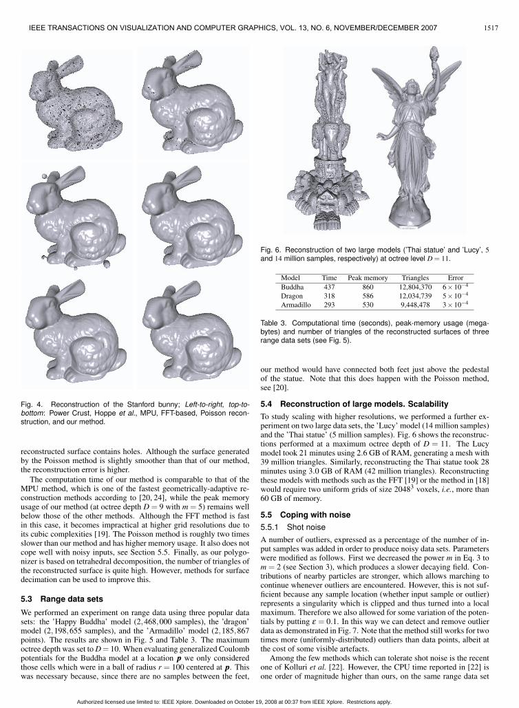
Fig. 4. Reconstruction of the Stanford bunny; Left-to-right, top-to-bottom: Power Crust, Hoppe et al., MPU, FFT-based, Poisson recon-struction, and our method.

reconstructed surface contains holes. Although the surface generatedby the Poisson method is slightly smoother than that of our method,the reconstruction error is higher.

The computation time of our method is comparable to that of theMPU method, which is one of the fastest geometrically-adaptive re-construction methods according to [20, 24], while the peak memoryusage of our method (at octree depth D = 9 with m = 5) remains wellbelow those of the other methods. Although the FFT method is fastin this case, it becomes impractical at higher grid resolutions due toits cubic complexities [19]. The Poisson method is roughly two timesslower than our method and has higher memory usage. It also does notcope well with noisy inputs, see Section 5.5. Finally, as our polygo-nizer is based on tetrahedral decomposition, the number of triangles ofthe reconstructed surface is quite high. However, methods for surfacedecimation can be used to improve this.

5.3 Range data sets

We performed an experiment on range data using three popular datasets: the ’Happy Buddha’ model (2,468,000 samples), the ’dragon’model (2,198,655 samples), and the ’Armadillo’ model (2,185,867points). The results are shown in Fig. 5 and Table 3. The maximumoctree depth was set to D = 10. When evaluating generalized Coulombpotentials for the Buddha model at a location ppp we only consideredthose cells which were in a ball of radius r = 100 centered at ppp. Thiswas necessary because, since there are no samples between the feet,

Fig. 6. Reconstruction of two large models (’Thai statue’ and ’Lucy’, 5

and 14 million samples, respectively) at octree level D = 11.

Model Time Peak memory Triangles Error

Buddha 437 860 12,804,370 6×10−4

Dragon 318 586 12,034,739 5×10−4

Armadillo 293 530 9,448,478 3×10−4

Table 3. Computational time (seconds), peak-memory usage (mega-bytes) and number of triangles of the reconstructed surfaces of threerange data sets (see Fig. 5).

our method would have connected both feet just above the pedestalof the statue. Note that this does happen with the Poisson method,see [20].

5.4 Reconstruction of large models. Scalability

To study scaling with higher resolutions, we performed a further ex-periment on two large data sets, the ’Lucy’ model (14 million samples)and the ’Thai statue’ (5 million samples). Fig. 6 shows the reconstruc-tions performed at a maximum octree depth of D = 11. The Lucymodel took 21 minutes using 2.6 GB of RAM, generating a mesh with39 million triangles. Similarly, reconstructing the Thai statue took 28minutes using 3.0 GB of RAM (42 million triangles). Reconstructingthese models with methods such as the FFT [19] or the method in [18]would require two uniform grids of size 20483 voxels, i.e., more than60 GB of memory.

5.5 Coping with noise

5.5.1 Shot noise

A number of outliers, expressed as a percentage of the number of in-put samples was added in order to produce noisy data sets. Parameterswere modified as follows. First we decreased the power m in Eq. 3 tom = 2 (see Section 3), which produces a slower decaying field. Con-tributions of nearby particles are stronger, which allows marching tocontinue whenever outliers are encountered. However, this is not suf-ficient because any sample location (whether input sample or outlier)represents a singularity which is clipped and thus turned into a localmaximum. Therefore we also allowed for some variation of the poten-tials by putting ε = 0.1. In this way we can detect and remove outlierdata as demonstrated in Fig. 7. Note that the method still works for twotimes more (uniformly-distributed) outliers than data points, albeit atthe cost of some visible artefacts.

Among the few methods which can tolerate shot noise is the recentone of Kolluri et al. [22]. However, the CPU time reported in [22] isone order of magnitude higher than ours, on the same range data set



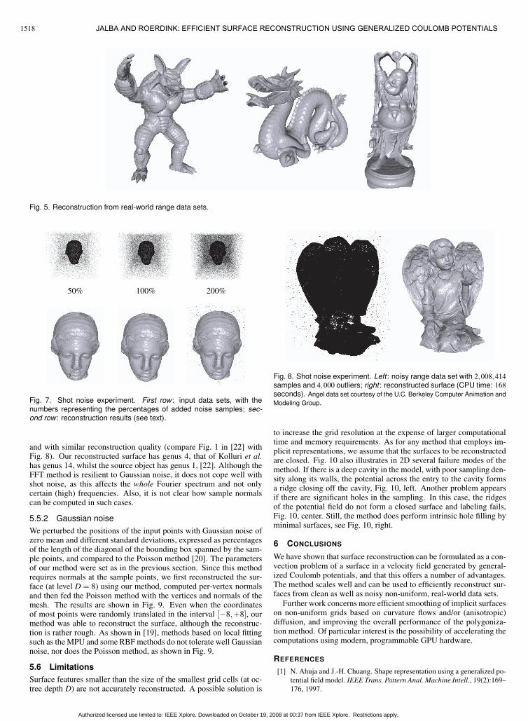
Fig. 5. Reconstruction from real-world range data sets.

50% 100% 200%

Fig. 7. Shot noise experiment. First row : input data sets, with thenumbers representing the percentages of added noise samples; sec-ond row : reconstruction results (see text).

and with similar reconstruction quality (compare Fig. 1 in [22] withFig. 8). Our reconstructed surface has genus 4, that of Kolluri et al.has genus 14, whilst the source object has genus 1, [22]. Although theFFT method is resilient to Gaussian noise, it does not cope well withshot noise, as this affects the whole Fourier spectrum and not onlycertain (high) frequencies. Also, it is not clear how sample normalscan be computed in such cases.

5.5.2 Gaussian noise

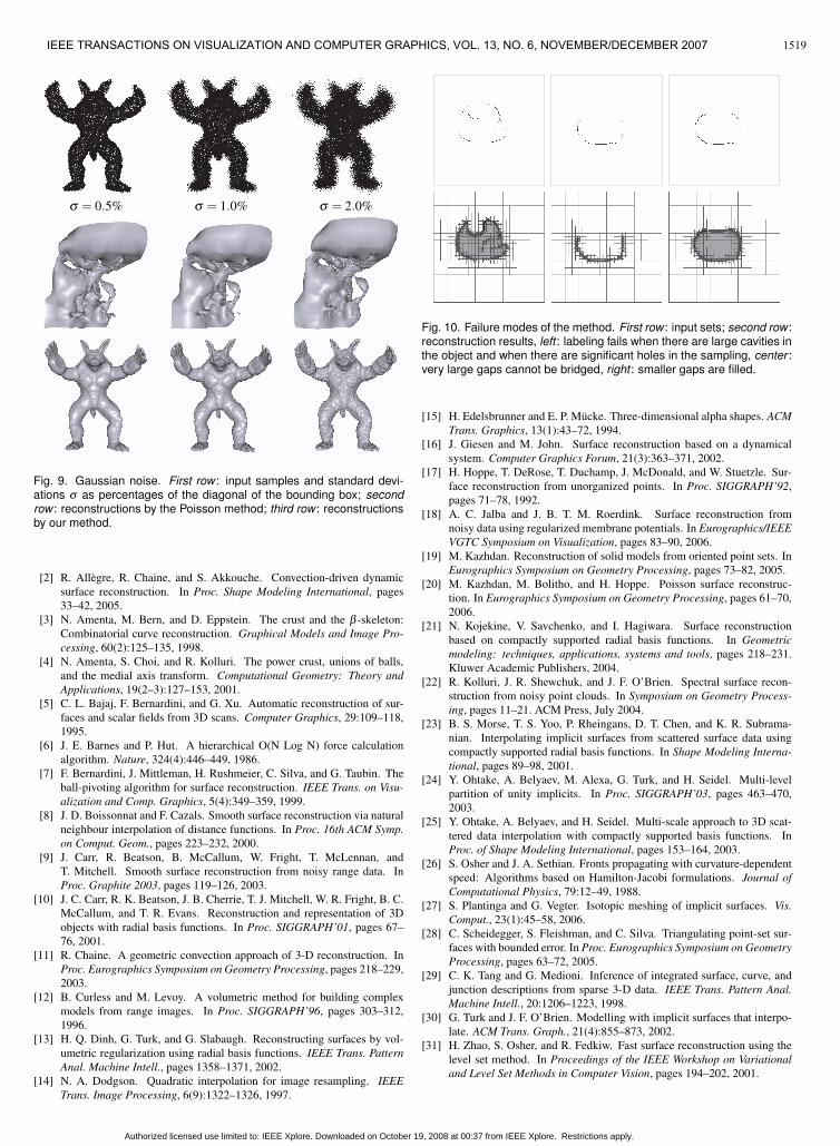
We perturbed the positions of the input points with Gaussian noise ofzero mean and different standard deviations, expressed as percentagesof the length of the diagonal of the bounding box spanned by the sam-ple points, and compared to the Poisson method [20]. The parametersof our method were set as in the previous section. Since this methodrequires normals at the sample points, we first reconstructed the sur-face (at level D = 8) using our method, computed per-vertex normalsand then fed the Poisson method with the vertices and normals of themesh. The results are shown in Fig. 9. Even when the coordinatesof most points were randomly translated in the interval [−8,+8], ourmethod was able to reconstruct the surface, although the reconstruc-tion is rather rough. As shown in [19], methods based on local fittingsuch as the MPU and some RBF methods do not tolerate well Gaussiannoise, nor does the Poisson method, as shown in Fig. 9.

5.6 Limitations

Surface features smaller than the size of the smallest grid cells (at oc-tree depth D) are not accurately reconstructed. A possible solution is

Fig. 8. Shot noise experiment. Left : noisy range data set with 2,008,414

samples and 4,000 outliers; right : reconstructed surface (CPU time: 168

seconds). Angel data set courtesy of the U.C. Berkeley Computer Animation and

Modeling Group.

to increase the grid resolution at the expense of larger computationaltime and memory requirements. As for any method that employs im-plicit representations, we assume that the surfaces to be reconstructedare closed. Fig. 10 also illustrates in 2D several failure modes of themethod. If there is a deep cavity in the model, with poor sampling den-sity along its walls, the potential across the entry to the cavity formsa ridge closing off the cavity, Fig. 10, left. Another problem appearsif there are significant holes in the sampling. In this case, the ridgesof the potential field do not form a closed surface and labeling fails,Fig. 10, center. Still, the method does perform intrinsic hole filling byminimal surfaces, see Fig. 10, right.

6 CONCLUSIONS

We have shown that surface reconstruction can be formulated as a con-vection problem of a surface in a velocity field generated by general-ized Coulomb potentials, and that this offers a number of advantages.The method scales well and can be used to efficiently reconstruct sur-faces from clean as well as noisy non-uniform, real-world data sets.

Further work concerns more efficient smoothing of implicit surfaceson non-uniform grids based on curvature flows and/or (anisotropic)diffusion, and improving the overall performance of the polygoniza-tion method. Of particular interest is the possibility of accelerating thecomputations using modern, programmable GPU hardware.

REFERENCES

[1] N. Ahuja and J.-H. Chuang. Shape representation using a generalized po-

tential field model. IEEE Trans. Pattern Anal. Machine Intell., 19(2):169–

176, 1997.



σ = 0.5% σ = 1.0% σ = 2.0%

Fig. 9. Gaussian noise. First row : input samples and standard devi-ations σ as percentages of the diagonal of the bounding box; secondrow : reconstructions by the Poisson method; third row : reconstructionsby our method.

[2] R. Allegre, R. Chaine, and S. Akkouche. Convection-driven dynamic

surface reconstruction. In Proc. Shape Modeling International, pages

33–42, 2005.

[3] N. Amenta, M. Bern, and D. Eppstein. The crust and the β -skeleton:

Combinatorial curve reconstruction. Graphical Models and Image Pro-

cessing, 60(2):125–135, 1998.

[4] N. Amenta, S. Choi, and R. Kolluri. The power crust, unions of balls,

and the medial axis transform. Computational Geometry: Theory and

Applications, 19(2–3):127–153, 2001.

[5] C. L. Bajaj, F. Bernardini, and G. Xu. Automatic reconstruction of sur-

faces and scalar fields from 3D scans. Computer Graphics, 29:109–118,

1995.

[6] J. E. Barnes and P. Hut. A hierarchical O(N Log N) force calculation

algorithm. Nature, 324(4):446–449, 1986.

[7] F. Bernardini, J. Mittleman, H. Rushmeier, C. Silva, and G. Taubin. The

ball-pivoting algorithm for surface reconstruction. IEEE Trans. on Visu-

alization and Comp. Graphics, 5(4):349–359, 1999.

[8] J. D. Boissonnat and F. Cazals. Smooth surface reconstruction via natural

neighbour interpolation of distance functions. In Proc. 16th ACM Symp.

on Comput. Geom., pages 223–232, 2000.

[9] J. Carr, R. Beatson, B. McCallum, W. Fright, T. McLennan, and

T. Mitchell. Smooth surface reconstruction from noisy range data. In

Proc. Graphite 2003, pages 119–126, 2003.

[10] J. C. Carr, R. K. Beatson, J. B. Cherrie, T. J. Mitchell, W. R. Fright, B. C.

McCallum, and T. R. Evans. Reconstruction and representation of 3D

objects with radial basis functions. In Proc. SIGGRAPH’01, pages 67–

76, 2001.

[11] R. Chaine. A geometric convection approach of 3-D reconstruction. In

Proc. Eurographics Symposium on Geometry Processing, pages 218–229,

2003.

[12] B. Curless and M. Levoy. A volumetric method for building complex

models from range images. In Proc. SIGGRAPH’96, pages 303–312,

1996.

[13] H. Q. Dinh, G. Turk, and G. Slabaugh. Reconstructing surfaces by vol-

umetric regularization using radial basis functions. IEEE Trans. Pattern

Anal. Machine Intell., pages 1358–1371, 2002.

[14] N. A. Dodgson. Quadratic interpolation for image resampling. IEEE

Trans. Image Processing, 6(9):1322–1326, 1997.

Fig. 10. Failure modes of the method. First row : input sets; second row :reconstruction results, left : labeling fails when there are large cavities inthe object and when there are significant holes in the sampling, center :very large gaps cannot be bridged, right : smaller gaps are filled.

[15] H. Edelsbrunner and E. P. Mucke. Three-dimensional alpha shapes. ACM

Trans. Graphics, 13(1):43–72, 1994.

[16] J. Giesen and M. John. Surface reconstruction based on a dynamical

system. Computer Graphics Forum, 21(3):363–371, 2002.

[17] H. Hoppe, T. DeRose, T. Duchamp, J. McDonald, and W. Stuetzle. Sur-

face reconstruction from unorganized points. In Proc. SIGGRAPH’92,

pages 71–78, 1992.

[18] A. C. Jalba and J. B. T. M. Roerdink. Surface reconstruction from

noisy data using regularized membrane potentials. In Eurographics/IEEE

VGTC Symposium on Visualization, pages 83–90, 2006.

[19] M. Kazhdan. Reconstruction of solid models from oriented point sets. In

Eurographics Symposium on Geometry Processing, pages 73–82, 2005.

[20] M. Kazhdan, M. Bolitho, and H. Hoppe. Poisson surface reconstruc-

tion. In Eurographics Symposium on Geometry Processing, pages 61–70,

2006.

[21] N. Kojekine, V. Savchenko, and I. Hagiwara. Surface reconstruction

based on compactly supported radial basis functions. In Geometric

modeling: techniques, applications, systems and tools, pages 218–231.

Kluwer Academic Publishers, 2004.

[22] R. Kolluri, J. R. Shewchuk, and J. F. O’Brien. Spectral surface recon-

struction from noisy point clouds. In Symposium on Geometry Process-

ing, pages 11–21. ACM Press, July 2004.

[23] B. S. Morse, T. S. Yoo, P. Rheingans, D. T. Chen, and K. R. Subrama-

nian. Interpolating implicit surfaces from scattered surface data using

compactly supported radial basis functions. In Shape Modeling Interna-

tional, pages 89–98, 2001.

[24] Y. Ohtake, A. Belyaev, M. Alexa, G. Turk, and H. Seidel. Multi-level

partition of unity implicits. In Proc. SIGGRAPH’03, pages 463–470,

2003.

[25] Y. Ohtake, A. Belyaev, and H. Seidel. Multi-scale approach to 3D scat-

tered data interpolation with compactly supported basis functions. In

Proc. of Shape Modeling International, pages 153–164, 2003.

[26] S. Osher and J. A. Sethian. Fronts propagating with curvature-dependent

speed: Algorithms based on Hamilton-Jacobi formulations. Journal of

Computational Physics, 79:12–49, 1988.

[27] S. Plantinga and G. Vegter. Isotopic meshing of implicit surfaces. Vis.

Comput., 23(1):45–58, 2006.

[28] C. Scheidegger, S. Fleishman, and C. Silva. Triangulating point-set sur-

faces with bounded error. In Proc. Eurographics Symposium on Geometry

Processing, pages 63–72, 2005.

[29] C. K. Tang and G. Medioni. Inference of integrated surface, curve, and

junction descriptions from sparse 3-D data. IEEE Trans. Pattern Anal.

Machine Intell., 20:1206–1223, 1998.

[30] G. Turk and J. F. O’Brien. Modelling with implicit surfaces that interpo-

late. ACM Trans. Graph., 21(4):855–873, 2002.

[31] H. Zhao, S. Osher, and R. Fedkiw. Fast surface reconstruction using the

level set method. In Proceedings of the IEEE Workshop on Variational

and Level Set Methods in Computer Vision, pages 194–202, 2001.



efﬁcient surface reconstruction using generalized...

Documents