effect of ambient pressure on diesel spray axial velocity and
TRANSCRIPT

Effect of Ambient Pressure on Diesel Spray AxialVelocity and Internal
Structure
Alan Kastengren, Christopher Powell Center for Transportation Research
Argonne National Laboratory
Kyoung-Su Im, Yujie Wang, and Jin Wang Advanced Photon Source
Argonne National Laboratory
DOE FreedomCAR & Vehicle TechnologiesProgram
Program Manager: Gupreet Singh

Good Understanding of Spray Structure isImportant in Diesel Combustion
�Performance and emissions of diesel engines are closely tied to the spray from the injector – Excessive penetration → wall wetting → UHC emissions – Poor spray pattern → poor fuel-air mixing → increased
emissions �Two of the most important variables that effect spray
behavior are injection pressure and ambient density– Penetration speed increased by higher injection pressure
and lower ambient density – Cone angle seems to increase as ambient density
increases
2
Current Spray Diagnostic Techniques AreInadequate
�Most spray measurements are based on optical measurements – Adequate for measuring penetration speed – Can’t probe internal spray structure in dense regions – Often not quantitative, due to strong scattering effects
�There are important parameters these optical techniques can’t show – Mass distribution of fuel in the spray – Fuel velocity away from the leading edge
�Need a nonintrusive, quantitative technique to measure sprays
3

X-Rays Give a Quantitative Determination ofFuel Distribution
N2 FlowX-Ray
Window
Fuel Injector
8 KeV X-ray Beam
I I0 Avalanche Photodiode
X-Y Slits 30 μm (V)
x200 μm (H)
I0 Incident x-ray intensity I = I e−MμM0
I Measured x-ray intensity μM Fuel absorption coefficient M = ln(I0 / I ) M Projected mass density, mass/area μM
4
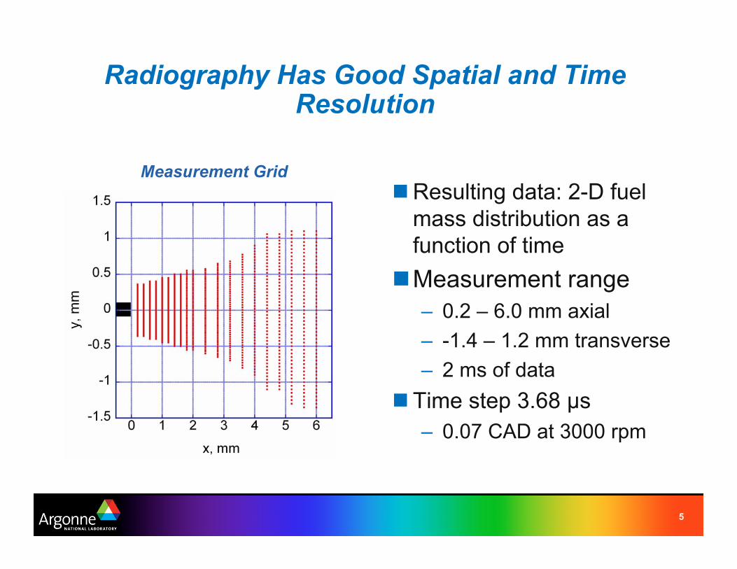
Radiography Has Good Spatial and TimeResolution
�Resulting data: 2-D fuel mass distribution as a function of time �Measurement range
– 0.2 – 6.0 mm axial – -1.4 – 1.2 mm transverse – 2 ms of data
�Time step 3.68 μs – 0.07 CAD at 3000 rpm
Measurement Grid
5

Experiment Details
� Light-duty diesel common-rail injector: solenoid driven
� Axial single hole – Non-hydroground: r/D = 0.2 – Orifice diameter 207 μm – L/D = 4.7
� Injection parameters – Injection pressure: 500 and 1000 bar – Injection duration: 1000 μs – Ambient gas: N2 at room temperature – Ambient pressure: 5 bar and 20 bar – Liquid: Diesel calibration fluid with
cerium additive
6
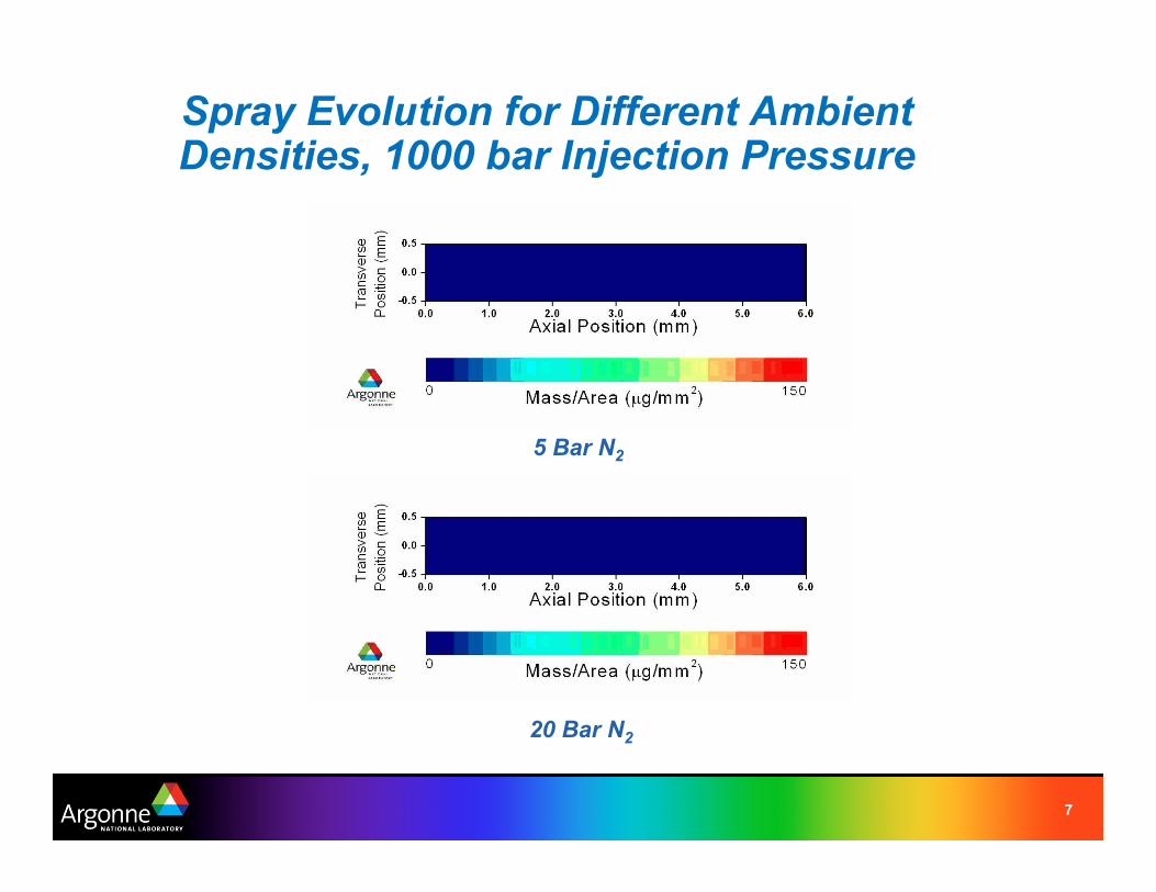
Spray Evolution for Different AmbientDensities, 1000 bar Injection Pressure
5 Bar N2
20 Bar N2
7
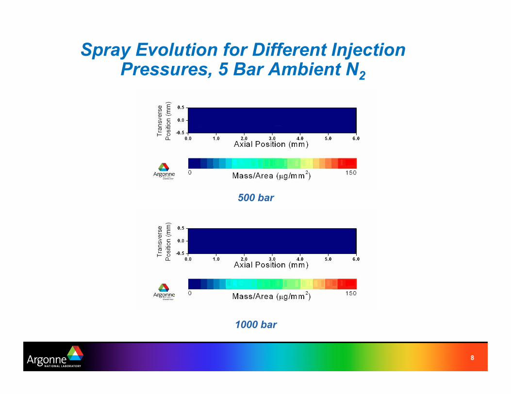
Spray Evolution for Different InjectionPressures, 5 Bar Ambient N2
500 bar
1000 bar
8

Penetration Results
�Penetration of leading edge vs. time � Increased ambient density
reduces penetration speed – Not as much as accepted
correlations indicate
� Lower injection pressure reduces penetration speed – More than expected
�Dynamics of injector opening are important to early penetration results Penetration
9

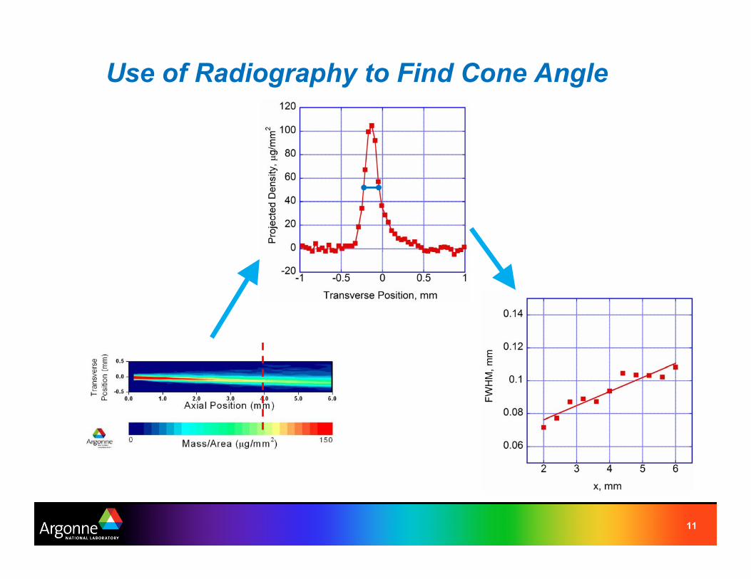
Previous Cone Angle Results
�Cone angle measurements help explain how the fuel mixes with the ambient gas �Typically found by examining optical spray images �X-ray radiography gives much more detail than optical
measurements on the internal mass distribution – Based on a well-defined, quantitative measure of the fuel
distribution – Can record cone angle as a function of time
10
Snapshot 100, 1000 bar, 5 bar
Use of Radiography to Find Cone Angle
11
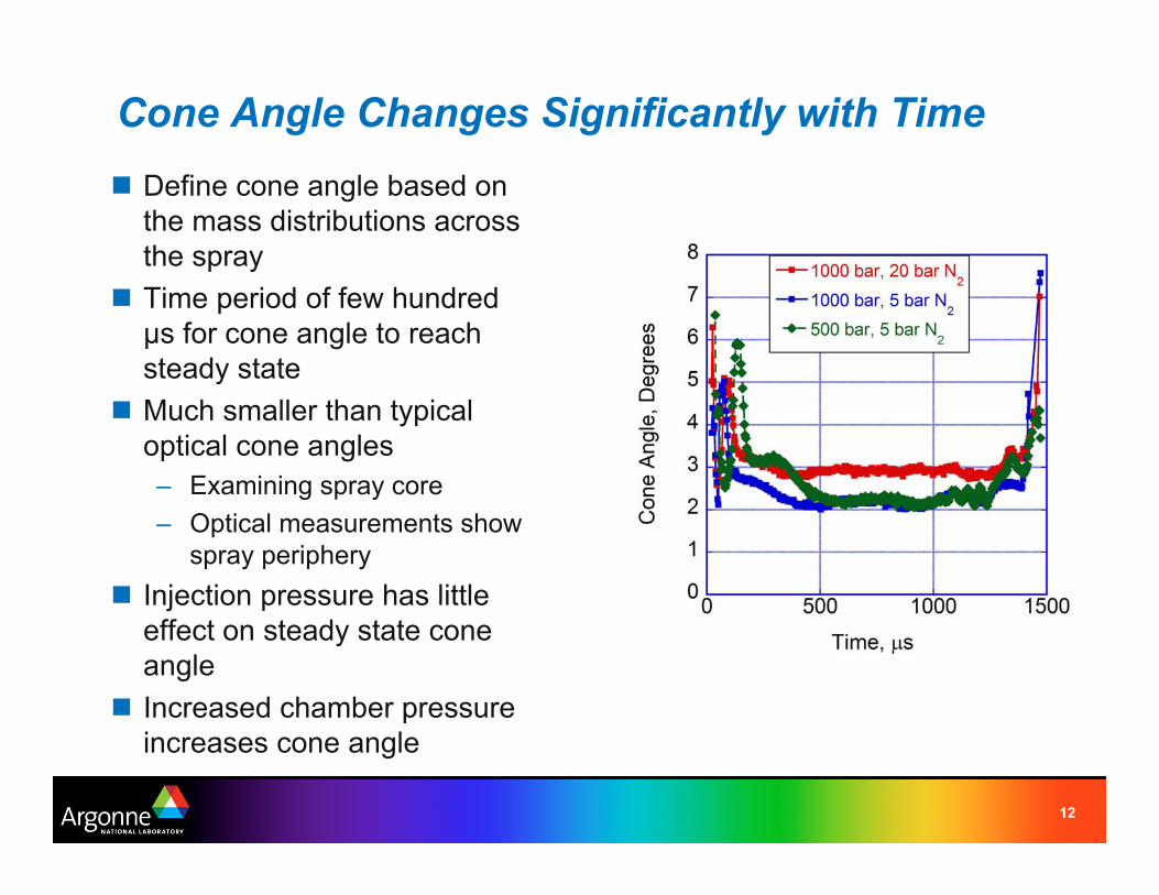
Cone Angle Changes Significantly with Time
� Define cone angle based on the mass distributions across the spray
� Time period of few hundred µs for cone angle to reach steady state
� Much smaller than typical optical cone angles – Examining spray core – Optical measurements show
spray periphery � Injection pressure has little
effect on steady state cone angle
� Increased chamber pressure increases cone angle
12
Spray Axial Velocity Determination
�Axial velocity of spray in dense regions of the spray is not well known �Axial velocity affects:
– Penetration speed – Shear with ambient gas – Initialize spray breakup models
�Radiography can be used to determine the mass-averaged axial velocity of the spray for limited time spans near the beginning of the spray event – Due to quantitative measurement of mass as a function of time – Velocity measured as a function of both x and t – Limited to time just after the start of injection
13
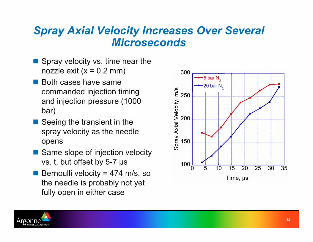
Spray Axial Velocity Increases Over SeveralMicroseconds
� Spray velocity vs. time near the nozzle exit (x = 0.2 mm)
� Both cases have same commanded injection timing and injection pressure (1000 bar)
� Seeing the transient in the spray velocity as the needle opens
� Same slope of injection velocity vs. t, but offset by 5-7 µs
� Bernoulli velocity = 474 m/s, so the needle is probably not yet fully open in either case
14

Spray Axial Velocity Is Strongly Affected byAmbient Density
� Spray velocity vs. x 33 µs after SOI
� Spray moves more slowly as distance from nozzle increases – Reduction in spray velocity due
to aerodynamic interactions
– Fluid at spray tip was injected at a slower velocity and so should move more slowly
� Difference in the two curves suggests that aerodynamic interactions slow the spray down more quickly with axial distance at higher ambient density
15

Future Work
�Continue to increase ambient pressure (density) of measurements – Further measurements at 30 bar ambient pressure in the near
future – Near the ambient density in-cylinder near TDC
�Perform measurements on multi-hole nozzles – More representative of applied nozzle geometries – More parameters to explore: spray angle, VCO vs. minisac
�Further refine the velocity determination – Improve signal/noise of measurements – Attempt to incorporate mechanical ROI measurements with the x-
ray density measurements
16

Future Work (cont.)
� Measurements on a heavy-duty HEUI injector – Full 6-hole production nozzle – Measurements in progress
� Measurements with biofuels – Completed initial measurements
with a biodiesel blend fuel � Dedicated transportation
applications x-ray facility under construction – Limited access to x-ray source in
the past – Dedicated facility will increase
access to x-ray source
17

),(),(),(
0
00 txTIM
txxmtxV cvma
>=&
Future Work: Spray Axial Velocity y Determination
Control Volume xz
Injector
Spray
x=x0
∞ ∞∞ ∞ m& cv (x > x0 , t) = − ∫ ∫ ρ(x0 , y, z, t) ⋅V (x0 , y, z, t) • n̂ ⋅ dz ⋅ dy ∫ ∫ ρ(x0, y, z, t) ⋅Vx (x0, y, z, t) ⋅ dz ⋅ dy
−∞ −∞ Vma (x0, t) = −∞ −∞ ∞ ∞ ∞ ⎡ ∞ ⎤
= ρ(x0 , y, z, t) ⋅Vx (x0 , y, z, t) ⋅ dz ⋅ dy ⎢ ρ(x0, y, z, t) ⋅ dz⎥ ⋅ dy∫ ∫ ∫ ∫⎢ ⎥−∞ −∞ −∞ ⎣−∞ ⎦
18