Effect of Assessment Scale on Spatial and TemporalVariations in CH4, CO2, and N2O Fluxes in a ForestedWetland

Zhaohua Dai & Carl C. Trettin & Changsheng Li &Harbin Li & Ge Sun & Devendra M. Amatya

Received: 3 March 2011 /Accepted: 6 June 2011# Springer Science+Business Media B.V. 2011

Abstract Emissions of methane (CH4), carbon dioxide(CO2), and nitrous oxide (N2O) from a forestedwatershed (160 ha) in South Carolina, USA, wereestimated with a spatially explicit watershed-scalemodeling framework that utilizes the spatial variationsin physical and biogeochemical characteristics acrosswatersheds. The target watershed (WS80) consisting ofwetland (23%) and upland (77%) was divided into 675grid cells, and each of the cells had unique combina-tion of vegetation, hydrology, soil properties, andtopography. Driven by local climate, topography, soil,and vegetation conditions, MIKE SHE was used togenerate daily flows as well as water table depth foreach grid cell across the watershed. Forest-DNDC wasthen run for each cell to calculate its biogeochemistryincluding daily fluxes of the three greenhouse gases

(GHGs). The simulated daily average CH4, CO2 andN2O flux from the watershed were 17.9 mg C, 1.3 g Cand 0.7 mg N m−2, respectively, during the period from2003–2007. The average contributions of the wetlandsto the CH4, CO2 and N2O emissions were about 95%,20% and 18%, respectively. The spatial and temporalvariation in the modeled CH4, CO2 and N2O fluxeswere large, and closely related to hydrological con-ditions. To understand the impact of spatial heteroge-neity in physical and biogeochemical characteristics ofthe target watershed on GHG emissions, we usedForest-DNDC in a coarse mode (field scale), in whichthe entire watershed was set as a single simulated unit,where all hydrological, biogeochemical, and biophys-ical conditions were considered uniform. The resultsfrom the field-scale model differed from those modeledwith the watershed-scale model which considered thespatial differences in physical and biogeochemicalcharacteristics of the catchment. This contrast demon-strates that the spatially averaged topographic orbiophysical conditions which are inherent with field-scale simulations could mask “hot spots” or smallsource areas with inherently high GHGs flux rates. Thespatial resolution in conjunction with coupled hydro-logical and biogeochemical models could play acrucial role in reducing uncertainty of modeled GHGemissions from wetland-involved watersheds.

Keywords Forest-DNDC . forested wetland .

greenhouse gases . carbon cycling

Water Air Soil PollutDOI 10.1007/s11270-011-0855-0

Z. Dai (*) :C. LiCSRC, EOS, University of New Hampshire,8 College Rd.,Durham, NH 03824, USAe-mail: zdai@fs.fed.us

Z. Dai : C. C. Trettin :H. Li :D. M. AmatyaCFWR, USDA Forest Service,3734 Highway 402,Cordesville, SC 29434, USA

G. SunEFETAC, SRS, USDA Forest Service,920 Main Campus Dr.,Raleigh, NC 27606, USA

1 Introduction

Wetlands, including forested wetlands, are an importantterrestrial methane (CH4) source and an importantcarbon (C) sink (Trettin and Jurgensen 2003). Under-standing production and consumption of C in wetland-dominated landscapes is important for estimating thecontribution of greenhouse gases (GHG), especiallyCO2, CH4, and N2O, to global warming. The generationand emission of GHGs from wetland-dominated land-scapes are closely related to inherent biogeochemicalprocesses which regulate the C balance (Rose andCrumpton 2006). However, those processes are stronglyinfluenced by vegetation, chemical, and physical soilproperties, geomorphology, and climate (Smemo andYavitt 2006).

The soil moisture regime is a key factor regulatingthe C balance and GHG flux in forests because itaffects aeration, and by extension determining whetherthe soil is aerobic or anaerobic. The soil environment,includingmoisture content, exhibits considerable spatialand temporal variation as a result of micro-topography,distribution of plant communities, climate, and soilproperties (Wang et al. 2000). Correspondingly, the Cbalance and GHG fluxes from soils should be expectedto exhibit considerable variation, especially in wetland-dominated landscapes (Sun et al. 2006).

The generation and consumption of CH4 from soilsare sensitive to soil aeration which is largely regulatedby the water table in wetlands (Trettin et al. 2006).However, the water table depth is not homogeneousacross a watershed because of topography, micro-topography, and surface geomorphic features. As aresult, there is a heterogeneous distribution of the soilrelative to the water table across a watershed (Sun et al.2006), which in turn suggests that the CH4 flux maycorrespond (Rask et al. 2002). These conditions arecharacteristic of many forested landscapes, especiallythose dominated by mosaics of uplands and wetlands.Accordingly, failure to consider the spatial heterogene-ity across a forest may induce significant errors whensimulating the C and GHG dynamics.

There have been a plethora of modeling studies toassess the soil C balance or GHG emissions over thepast decades, and the common approach is to utilize afield-scale model to simulate one cell or catchmentwith averaged field conditions (Pansu et al. 2004).

The size of the cell or catchment has variedconsiderably from plots (e.g., hundreds of m2), towatersheds (e.g., hundreds of ha) or basins (hundredsof km2) (Shindell et al. 2004; Huang et al. 2006). Theapplication of a field-scale biogeochemical modelingapproach across a large area will obviously overlookinherent spatial variability in the soil environment andpotentially incur significant errors in predicting the Cand GHG dynamics at the scale of assessment, suchas over or under predicting GHG fluxes due to spatialheterogeneity in biophysical and biogeochemicalcharacteristics regulating C balance. This conse-quence reflects the fact that while explicit informationon spatial and temporal hydrologic dynamics is criticalfor simulating C and GHG dynamics in forestedwetlandsoils, few biogeochemical models have the capability toaccurately consider hydrologic dynamics across spaceand time. One of the solutions is to obtain the spatial andtemporal hydrologic dynamics by means of physicallybased hydrologic models (Sun et al. 2006). Thisapproach is applicable to a wide range of watershedconditions. Therefore, linking a physically baseddistributed hydrologic model to a watershed-scalebiogeochemical modeling tool for estimating dynamicC, N, and GHG in forested catchments should providean improved basis for assessing C and GHG dynamicsin forested systems.

This paper reports the effort to (1) quantify CH4,soil CO2 and N2O fluxes for a 160 ha forestedwatershed on the Santee Experimental Forest locatedin the lower coastal plain of South Carolina, USA,and (2) assess the differences in simulated GHGdynamics for the mosaic landscape consisting ofwetlands and uplands using two biogeochemicalmodeling approaches, a field-scale model whichemploys spatial average conditions from the studysite and a watershed-scale model which utilizesspatial and temporal characteristics within the water-shed. This study used the biogeochemical model,Forest-DNDC (Li et al. 2000; Stang et al. 2000), anda hydrology model, MIKE SHE (DHI 2005). Theresults are used to contrast the spatial and temporalvariations of GHG fluxes in the watershed to assessthe impact of spatial heterogeneity in biophysical andbiogeochemical conditions on estimating C and GHGdynamics in the landscapes with complex character-istics of topography, hydrology, soils, and vegetation.

Water Air Soil Pollut

2 Materials and Methods

2.1 Watershed Description

The study site is a first-order watershed (WS80)containing both uplands and wetlands, located at33.15° N, 79.8° W on Santee Experimental Forest,55 km northwest of Charleston, South Carolina (Fig. 1).WS80 (160 ha) serves as the control catchment for apaired watershed system within the second-order water-shed (WS79, 500 ha) draining into Huger Creek, atributary of East Branch of the Cooper River. Thisreference forest has gauging records since 1967. It ischaracteristic of the subtropical region of the southeast-ern Atlantic Coast with short, warm, and humid wintersand long and hot summers; the annual average temper-ature is 18.7°C, and the mean annual precipitation(1971–2000) is 1,350 mm (Amatya et al. 2003). Thetopography is planar, and the slope is less than 4%. Theelevation is between 4 and 10 m above mean sea level.The site has a shallow water table, and about 23% of thewatershed is classified as wetlands (Sun et al. 2000).

The soils in the catchment are typified by a loamsurface and clayey subsoil, which is moderately wellto somewhat poorly drained in the upland and poorly

drained in the riparian zone (Long 1980). Claycontent is ≤30% in topsoil (within 30 cm), 40–60%in subsoil (>30 cm) (Long 1980). Soil reaction isacidic; pH is between 4.5 and 6.5.

As is a reference watershed, the forest on WS80 hasnot been managed in more than five decades. However,the forest was heavily impacted by Hurricane Hugo in1989. This site remained unmanaged after the hurricane,without biomass removal or salvage logging. The currentforest stand is from residuals and natural regeneration.The current forest cover type consists of bottomlandhardwoods in the riparian zone and mixed pine-hardwoods elsewhere (Hook et al. 1991; Harder et al.2007). The dominant trees are loblolly (Pinus taeda L.),sweetgum (Liquidambar styraciflua), and a variety ofoak species (Queercus spp.) (Hook et al. 1991; Harderet al. 2007).

2.2 Data Collections and Field Measurements

Precipitation in WS80 was measured using anautomatic tipping bucket and a manual rain gauge asa backup. Air and soil temperatures, CO2 emission,and soil moisture were also measured on-site, andused to assess Forest-DNDC performance. Additional

Fig. 1 Watershed WS80 onAtlantic Coastal Plain,South Carolina, USA(WS79 (500°ha) is dividedinto three parts; they areWS77 (155°ha), WS80(160 ha), and the part(WS79b) between WS77and WS80, respectively)

Water Air Soil Pollut

meteorological measurements, including solar and netradiations, wind speed, wind direction, vapor pres-sure, and relative humidity were collected at 30-minintervals at a weather station at Santee ExperimentalForest Headquarters (SEFH) about 3 km away fromWS80. The data from SEFH were processed toestimate daily potential evapotranspiration (PET)(Xu and Singh 2005). Except for leaf area index(LAI) calculated based on leaf biomass measurements(Lloyd and Olson 1974; Bréda 2003) in this studyarea for 2 years, LAI was also measured periodicallythroughout 2 years using a LiCOR-2000 plant canopyanalyzer. Both PET and LAI were used for modelinghydrologic dynamics in the watershed.

Water table depth data were measured at twoautomatic recording wells (WL40) installed in anupland area and a lowland location to record watertable elevation at 4-h intervals and by eight manualwells installed across the watershed with biweeklymeasurements (Fig. 1). An automatic Teledyne ISCO-4210 flow meter measured stream gauge heightsabove a compound V-notch weir at 10-min intervals.The discharge was calculated using a standard ratingcurve method developed for the compound weir, andintegrated into daily and monthly values, and thenconverted from m3 s−1 to mm d−1 to compare withdaily precipitation. Both the measured water tabledepth and discharge were used to calibrate andvalidate the hydrologic parameters.

2.3 Forest-DNDC Model

Forest-DNDC is a process-based biogeochemicalmodel, which is used to predict plant growth andproduction, C and N balance, and generation andemission of greenhouse gases (CO2, CH4, and N2O)by means of simulating C and N dynamics in forestecosystems (Li et al. 2000; Stang et al. 2000; Miehleet al. 2006). The model integrates decomposition,nitrification–denitrification, photosynthesis, andhydrothermal balance in forest ecosystems. Thesecomponents are mainly driven by environmentalfactors, including climate, soil, vegetation, and humanactivities. The model has been tested and used forestimating GHG emission from forested ecosystemsin a wide climatic region, including boreal, temperate,subtropical, and tropical (Stang et al. 2000; Zhang etal. 2002; Li et al. 2004; Kiese et al. 2005, 2006;Kurbatova et al. 2008).

In order to better understand the impact of thespatial heterogeneity in biophysical and biogeochem-ical conditions on GHG emissions from forestedecosystems with mosaic landscape consisting ofuplands and wetlands, Forest-DNDC was modifiedto explicitly represent spatial complexities in hydro-geological and climatic characteristics, and soil andvegetation types at watershed or regional scales.

2.4 Linking Hydrologic Model MIKE SHE

MIKE SHE (Abbott et al. 1986a, b; Graham and Butts2005), a distributed and physically based hydrologicmodeling system, was linked to Forest-DNDC toprovide spatially explicit dynamic hydrologic infor-mation. MIKE SHE has the capability of simulatingall major terrestrial hydrologic processes, including 3-D water movement in soil profile, 2-D watermovement of overland flow and 1-D water movementin rivers/streams, and evapotranspiration (ET) (DHI2005). It is flexibly applicable at various spatialscales, ranging from a simple soil profile to largeriver basins or regions with complex hydro-geologiccharacteristics (Graham and Butts 2005), and widelyused to simulate watershed-scale hydrology (Sahoo etal. 2006; Mernild et al. 2008; Vázquez et al. 2008;Zhang et al. 2008; Lu et al. 2011). MIKE SHE hasbeen tested to simulate hydrology for this watershed(Dai et al. 2010). Accordingly, it is an appropriatemodel to supply spatially and temporally dynamichydrologic information to Forest-DNDC.

An interface was developed to transfer the MIKESHE-modeled hydrological data to Forest-DNDC,which included daily water table depth, overland flowand subsurface flow for the entire watershed. MIKESHE and Forest-DNDC shared a set of same GIS-based files. Elevation and other relevant topographicparameters were defined for each of the grid cellsbased on the WS80 DEM data.

2.5 Model setup and Parameterizations

The MIKE SHE model framework was configured tosimulate dynamic water table in space and time anddischarge in time. It was coupled with routing flowmodel MIKE 11, a one-dimensional river/channelwater movement model. The data files for thesimulation model setup were primarily grid and/orshape format for spatial data, including vegetation,

Water Air Soil Pollut

soil, and stream network. The other data files weretime series data for precipitation and PET. MIKE SHEmodel setup for hydrologic modeling in this water-shed was described in details by Dai et al. (2010).

Forest-DNDC was set to simulate C and N dynamicsfor forested wetlands (Li et al. 2004). Data files were inASCII format, including climate, hydrology, soil, andvegetation. A set of two-dimensional grid files werecreated for the spatial variation in hydrology, soil andvegetation. For this study, every grid file was a datasetwith 675 cells, and each cell represented 0.25 ha (50×50 m) of the watershed. In order to identify thewetland’s contribution to methane emissions from thiswatershed, the site was divided into wetlands (∼23% ofthe watershed area with water table level of ≥0 in wetperiods) and uplands (77%) to reflect the mosaictopography mixed with wetlands and uplands basedon the water table depth during a normal wet periodin 2003.

The watershed-scale simulations used the spatialand temporal water table dynamics represented by675 cells within WS80. The field-scale approachemployed daily mean water table which was calculatedfrom the 675 cells. To assess the relative contributions ofwetland and upland ecosystems within the watershed,the field-scale simulations used the daily mean watertable depth for the wetland cells (155) and upland cells(520). The watershed-scale model was utilized toestimate contributions of wetlands and uplands at thewatershed scale using a dynamic water table for thecorresponding cells. The other spatially biophysical andbiogeochemical characteristics of the catchment weredirectly employed by the watershed scale, and theirspatial average conditions were used by the field scale.

3 Results and Discussion

3.1 Calibration and Validation

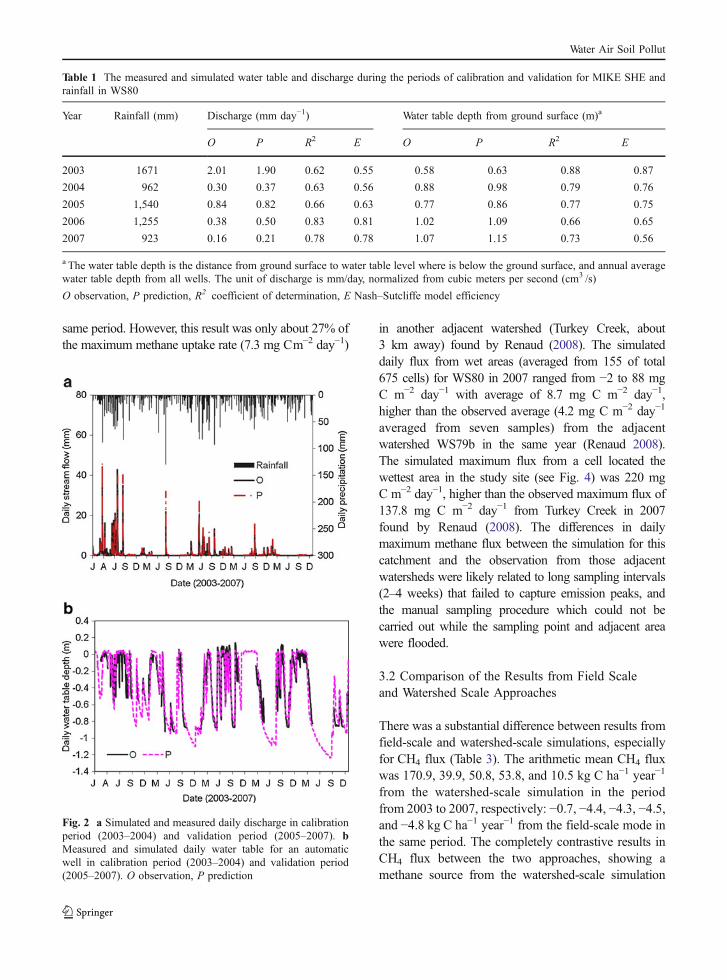
Based on a hydrology study on WS80 by Dai et al.(2010), MIKE SHE did an excellent job representingthe variations of the water table and stream discharge(Table 1; Fig. 2). The simulated water table depth anddischarge were in agreement with observations withthe model performance efficiency (E≤1) (Nash andSutcliffe, 1970) values ranging between 0.55 and 0.78for discharge and 0.55–0.87 for water table depth aswell as their R2 values ranging between 0.62 and 0.83

for discharge and 0.66 and 0.88 for water table depth(Dai et al. 2010). These results demonstrate a soundbasis for using MIKE SHE to provide the hydrologiccontext for biogeochemical simulations.

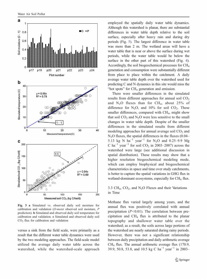
Forest-DNDC was calibrated and validated usingsoil CO2 flux, soil temperature and soil moisture.While there was general agreement between the fieldmeasurements and simulated values (Fig. 3; Table 2),there were small consistent differences. The simulatedsoil temperature and CO2 flux tended to be slightlylower than the field measurements, and the simulatedsoil moisture was slightly higher than the fieldmeasurements during wet periods. These differencesmay be related to the location and distribution of themeasurement plots, which include both upland andwetland. It may also be influenced by the micro-topography within a measurement plot, whereby thefour to six measurement points used on a plot wereinadequate to representative the inherent variationwithin a plot. The distribution of measurement pointstended to be on the slightly higher (i.e., 10–20 cm)micro-topographic positions, which would not besubmerged during periods of high water table,although those events are not uncommon. Since thesimulated results represent an average across the plot,it is reasonable that the simulated soil moisture couldbe higher than the measured values for wet periods,especially in the riparian zone.

The simulated soil temperature was in agreement withthe measurements with a proper model performanceefficiency (Nash and Sutcliffe 1970) being E=0.61 forthe model calibration and E=0.83 for the validation(Fig. 3b; Table 2). Although there were some differencesbetween observation and simulation, these figures(Fig. 3; Table 2) also showed that Forest-DNDCcaptured the spatial and temporal variation in soiltemperature and CO2 dynamics across the watershed.The E was 0.42–0.70 and R2 was 0.44–0.83 (Table 2)from Forest-DNDC model calibration and validation.These results showed that Forest-DNDC was applicablefor estimating the spatial distribution of GHG emissionswith proper model efficiency.

The simulated daily CH4 flux was also comparableto the measurements from adjacent watersheds.Renaud (2008) found that the minimum daily methaneflux was −1.9 mg C m−2 from WS79b (an adjacentwatershed, about 200 m away from the measurementplot to our study site) in Nov. of 2007, approximate tothe simulated value (−2 mg C m−2 day−1) for WS80 in

Water Air Soil Pollut

same period. However, this result was only about 27% ofthe maximum methane uptake rate (7.3 mg Cm−2 day−1)

in another adjacent watershed (Turkey Creek, about3 km away) found by Renaud (2008). The simulateddaily flux from wet areas (averaged from 155 of total675 cells) for WS80 in 2007 ranged from −2 to 88 mgC m−2 day−1 with average of 8.7 mg C m−2 day−1,higher than the observed average (4.2 mg C m−2 day−1

averaged from seven samples) from the adjacentwatershed WS79b in the same year (Renaud 2008).The simulated maximum flux from a cell located thewettest area in the study site (see Fig. 4) was 220 mgC m−2 day−1, higher than the observed maximum flux of137.8 mg C m−2 day−1 from Turkey Creek in 2007found by Renaud (2008). The differences in dailymaximum methane flux between the simulation for thiscatchment and the observation from those adjacentwatersheds were likely related to long sampling intervals(2–4 weeks) that failed to capture emission peaks, andthe manual sampling procedure which could not becarried out while the sampling point and adjacent areawere flooded.

3.2 Comparison of the Results from Field Scaleand Watershed Scale Approaches

There was a substantial difference between results fromfield-scale and watershed-scale simulations, especiallyfor CH4 flux (Table 3). The arithmetic mean CH4 fluxwas 170.9, 39.9, 50.8, 53.8, and 10.5 kg C ha−1 year−1

from the watershed-scale simulation in the periodfrom 2003 to 2007, respectively: −0.7, −4.4, −4.3, −4.5,and −4.8 kg C ha−1 year−1 from the field-scale mode inthe same period. The completely contrastive results inCH4 flux between the two approaches, showing amethane source from the watershed-scale simulation

Fig. 2 a Simulated and measured daily discharge in calibrationperiod (2003–2004) and validation period (2005–2007). bMeasured and simulated daily water table for an automaticwell in calibration period (2003–2004) and validation period(2005–2007). O observation, P prediction

Table 1 The measured and simulated water table and discharge during the periods of calibration and validation for MIKE SHE andrainfall in WS80

Year Rainfall (mm) Discharge (mm day−1) Water table depth from ground surface (m)a

O P R2 E O P R2 E

2003 1671 2.01 1.90 0.62 0.55 0.58 0.63 0.88 0.87

2004 962 0.30 0.37 0.63 0.56 0.88 0.98 0.79 0.76

2005 1,540 0.84 0.82 0.66 0.63 0.77 0.86 0.77 0.75

2006 1,255 0.38 0.50 0.83 0.81 1.02 1.09 0.66 0.65

2007 923 0.16 0.21 0.78 0.78 1.07 1.15 0.73 0.56

a The water table depth is the distance from ground surface to water table level where is below the ground surface, and annual averagewater table depth from all wells. The unit of discharge is mm/day, normalized from cubic meters per second (cm3 /s)

O observation, P prediction, R2 coefficient of determination, E Nash–Sutcliffe model efficiency

Water Air Soil Pollut

versus a sink from the field scale, were primarily as aresult that the different water table dynamics were usedby the two modeling approaches. The field-scale modelutilized the average daily water table across thewatershed, while the watershed-scale approach

employed the spatially daily water table dynamics.Although this watershed is planar, there are substantialdifferences in water table depth relative to the soilsurface, especially after heavy rain and during dryperiods (Fig. 5). The largest difference in water tablewas more than 2 m. The wetland areas will have awater table that is near or above the surface during wetperiods, while the water table would be below thesurface in the other part of this watershed (Fig. 4).Accordingly, the soil biogeochemical processes for CH4

generation and consumption were substantially differentfrom place to place within the catchment. A dailyaverage water table depth over the watershed used forpredicting C and N dynamics in this site would miss the“hot spots” for CH4 generation and emission.

There were smaller differences in the simulatedresults from different approaches for annual soil CO2

and N2O fluxes than for CH4, about 25% ofdifference for N2O, and 10% for soil CO2. Thesesmaller differences, compared with CH4, might showthat soil CO2 and N2O were less sensitive to the smallchanges in water table depth. Despite of the smallerdifferences in the simulated results from differentmodeling approaches for annual average soil CO2 andN2O fluxes, the spatial differences in the fluxes (0.04–5.13 kg N ha−1 year−1 for N2O and 0.25–9.9 MgC ha−1 year−1 for soil CO2 in 2003–2007) across thewatershed were large (see additional discussion inspatial distribution). These results may show that ahigher resolution biogeochemical modeling mode,which can employ biophysical and biogeochemicalcharacteristics in space and time over study catchments,is better to capture the spatial variations in GHG flux inwetland-dominant ecosystems, especially for CH4 flux.

3.3 CH4, CO2, and N2O Fluxes and their Variationsin Time

Methane flux varied largely among years, and theannual flux was positively correlated with annualprecipitation (P<0.01). The correlation between pre-cipitation and CH4 flux is attributed to the planartopography and shallower water table over thewatershed; as a result, the soils across large portions ofthe watershed are nearly saturated during rainy periods.However, there was not a significant relationshipbetween daily precipitation and daily arithmetic averageCH4 flux. The annual arithmetic average flux (170.9,39.9, 50.8, 53.8, and 10.5 kg C ha−1 year−1 in 2003–

Fig. 3 a Simulated vs. observed daily soil moisture forcalibration and validation (O-moist observed soil moisture, Pprediction). b Simulated and observed daily soil temperature forcalibration and validation. c Simulated and observed daily soilCO2 flux for calibration and validation

Water Air Soil Pollut

2007) was larger than the median (122, 8, 11, 12,and −2 kg C ha−1 year−1), about 30% higher than themedian in 2003, an extreme wet year, and about 80%higher in other climatic years (Table 3). Thisdifference was related to the heterogeneously spatialdistribution of CH4 flux associated with spatial watertable distribution influenced by topography.

The average N2O flux was 2.16–3.04 kgN ha−1 year−1, the median was 2.13–3.20, andgeometric mean was 1.58–2.87 in the 5-year period(2003–2007) (Table 3). The arithmetic mean wasslightly higher than geometric value, only about 12%on average. The variation of year-to-year N2O fluxwas much smaller than for CH4. The increase in N2Oemissions in dry years is attributed to an increase insoil organic matter decomposition and a decrease inplant N uptake.

Soil CO2 flux in this watershed was obviouslyaffected by climatic conditions. The flux in 2003 (a

wet year, 320 mm of precipitation was higher than thelong-term average of 1,350 mm) was about 33.4% ofthe flux in 2007 (a dry year, 430 mm of precipitation wasless than the long-term average, 750 mm less than theprecipitation in 2003). The difference in soil CO2 fluxbetween wet and dry years showed that the soilrespiration in wet years was substantially lower thandry years. It was shown that soil respiration wasinfluenced by changes in soil moisture. Annual soilCO2 flux was significantly and linearly correlated (p<<0.01) to the annual mean water table in the watershed(Fig. 6), the higher annual average water table, the lowerannual mean soil CO2 flux. High soil CO2 flux in dryyears is primarily as wetlands loss to a decrease in thewater table level regulated by precipitation in this forest.This result was similar to the finding of Pietsch et al.(2003) that water table level decrease in their sites led toan increase in soil carbon loss.

The pattern of daily soil CO2 flux was seasonal.The high daily soil CO2 flux occurred in summersalthough precipitation did influence the flux. Thechanges in soil CO2 flux were primarily as a result ofincreasing soil temperature in the summer, andchanges in precipitation associated with altering soilmoisture regime increasing or decreasing soil respiration.Although the effect of water table on daily soil CO2 fluxwas similar with annual flux, the relationship betweendaily soil CO2 flux and daily water table depth wasdifferent from that between annual average soil CO2

flux and annual average water table depth, appearing tobe a semi-logarithmic relationship (Fig. 7).

3.4 Spatial Variations

The spatial variation of CH4 flux in the watershed waslarge (Fig. 8a). The flux spatially ranged from −4

Table 2 Observed and simulated soil temperature, moisture, and CO2 for the calibration and validation of Forest-DNDC

Modeling Items O P R2 E

Calibration Temperature (°C) 23.5 22.3 0.68 0.61

Moisture (m3 m−3) 0.42 0.41 0.83 0.68

Soil CO2 (kg C ha−1 day−1) 66.6 62.2 0.63 0.55

Validation Temperature (°C) 19.7 19.9 0.83 0.83

Moisture (m3 m−3) 0.54 0.53 0.44 0.42

Soil CO2 (kg C ha−1 day−1) 39.6 39.4 0.66 0.61

O observation, P prediction, Soil CO2 the CO2 which includes organic matterdecomposition in soil and forest floor, root respiration, and moss respiration

Fig. 4 Water table level in the wet period of 2003 (a week aftera heavy rain)

Water Air Soil Pollut

to +716, −4 to +332, −4 to +590, −4 to +384, and −5to +114 kg C ha−1 year−1 in the watershed in 2003–2007, respectively. The difference in CH4 flux acrossthe watershed was related to the topography. Thehigh CH4 flux occurred at the places that were veryflat or depressional, thereby holding topsoil saturatedfor a long time during wet periods. There was no ornegative CH4 flux on surfaces with slope (≥1%), andin general the flux was low across most of the placesin the watershed. Therefore, CH4 flux in space washeterogeneous in the watershed, the distribution wasskewed (Fig. 8b). This result was similar with that

reported by Trettin and others (2006), a geometricaverage for CH4 flux was much less than thearithmetic mean. Although CH4 flux distribution inthe wetland was skewed, geometric average was notavailable for this catchment since there were zeroand negative fluxes for CH4. Therefore, the medianof CH4 flux should be better than arithmetic averageto reflect the mean level of CH4 flux in thewatershed for normal and wet years. However,the median was not good for dry years, such as2007. The median was −2 kg C ha−1 year−1 in2007, an extreme dry year, which indicated that thiscatchment was overall a methane sink. However, thetotal methane emission from wetlands (2 Mg C) in

Table 3 Simulated annual CH4, soil CO2, and N2O fluxes in WS80 (2003–2007)*

Year 2003 2004 2005 2006 2007 Mean

CH4-a (kg C ha−1 year−1) 170.9 39.9 50.8 53.8 10.5 65.2

CH4-m(kg C ha−1 year−1) 122.0 8.0 11.0 12.0 −2.0 31.0 (13.0)a

CH4-f (kg C ha−1 year−1) −0.7 −4.4 −4.3 −4.5 −4.8 −3.7N2O-a (kg N ha−1 year−1) 2.16 3.04 2.34 2.26 2.47 2.45

N2O-m (kg N ha−1 year−1) 2.13 3.20 2.37 2.20 2.53 2.49 (2.47)a

N2O-g (kg N ha−1 year−1) 1.58 2.87 2.12 2.11 2.39 2.21

N2O-f (kg N ha−1 year−1) 2.32 2.48 1.57 1.57 1.56 1.90

Soil CO2-a (Mg C ha−1 year−1) 2.48 5.37 3.41 4.58 7.42 4.65

Soil CO2-m (Mg C ha−1 year−1) 2.51 5.39 3.27 4.52 7.40 4.62 (4.83)a

Soil CO2-g (Mg C ha−1 year−1) 1.91 4.78 2.73 3.99 7.21 4.13

Soil CO2-f (Mg C ha−1 year−1) 2.51 5.36 3.39 4.74 7.96 4.79

There was no geometric average for CH4 because there were zero and negative fluxes in space in the watershed

-a arithmetic average from watershed scale, -g geometric average from watershed scale, -m median, -f result from field-scale modela The value in braces is the median obtained from all results simulated by watershed-scale model for the 5-year period (2003–2007);the value out of the braces is arithmetically averaged from five yearly medians

Fig. 5 Water table in a dry period on WS80Fig. 6 The relationship between annual soil CO2 flux andannual mean water table on WS80

Water Air Soil Pollut

2007 was much higher than the uptake in uplands(0.4 Mg C).

The CH4 fluxes from wetland and upland compo-nents of WS80 were simulated using the watershed-

scale model with spatially distributed water tabledynamics within each component. The arithmeticmean flux was 425, 125, 168, 150, and 31 kgC ha−1 year−1 from the wetlands and 32, 4, 18, 6,and 0 from uplands for 2003, 2004, 2005, 2006, and2007, respectively. The CH4 flux from wetlands wasover 90% of the total flux from this watershed. Theresults from these divisions demonstrated that thewetlands were the dominant CH4 source. The smallamount of CH4 from uplands was primarily as theresult that the topsoil in a large area of this catchmentwas saturated during wet periods due to this water-shed having a shallow water table and flat topographyand that their some places are adjacent to wetlands.

The CH4 flux from field-scale modeling foruplands (−3.7, −4.4, −4.3, −4.5, and −4.7 kgC ha−1 year−1) was significantly lower than thosefrom the watershed-scale approach (32, 4, 18, 6, and

Fig. 8 a Spatial distribution of annual methane flux on WS80in 2006. b Distribution frequency of methane flux over thewatershed in 2003

Fig. 7 Effect of daily water table on daily soil CO2 flux infive plots

Fig. 9 a Spatial distribution of soil CO2 flux on WS80 in 2003.b Distribution frequency of soil CO2 flux over the watershedin 2003

Water Air Soil Pollut

0 kg C ha−1 year−1). However, there was a smalldifference in methane flux from wetlands betweentwo approaches (425, 125, 168, 150, and 31 kg Cha−1 year−1 simulated by the watershed scale and497.4, 114.6, 105.8, 123.6 ,and 32.1 modeled by thefield scale). The large difference in CH4 flux fromuplands between the two approaches is due to largedifferences in water table level location to location.Therefore, the average water table condition fromuplands dismissed CH4 emissions from the uplandedges near the riparian zone and those flat areaswhere the soils were saturated during wet periods. Anapproximate CH4 flux from the wetland areas pre-dicted by both the field-scale and watershed-scalemodeling approaches is primarily as a result ofshallow water table and planar topography, especiallywithin wetlands. The topsoil in wetlands is saturatedduring wet periods in this watershed, but the topsoilin uplands is only saturated in the durations withconsecutively proper precipitation and becomes un-saturated rapidly after raining. The difference in watertable within most of wetlands is small. The spatialdifference in CH4 flux in this catchment showed thesubstantial impact of spatial heterogeneity in thebiogeochemical conditions within the catchments ongeneration and emission of methane. These resultsindicated that the consideration of the spatial hetero-geneity across a catchment, especially across a largecatchment with mosaics of wetlands and uplands, wasneeded to estimate C balance and GHG emissions inwetland-dominated landscape ecosystems. Althoughthe uncertainty of modeling GHG emissions fromwetland-dominated watersheds can be reduced byusing the high resolution modeling approach, thedata input requirements for each cell and computationtime are onerous. Accordingly, an alternative is todivide the catchment into several sub-catchments toreflect major differences in hydrology, soils, vegetation,and topography.

The flux of soil CO2 spatially ranged from 0.25 to5.7, 0.73 to 6.9, 0.32 to 7.5, 0.88 to 7.8, and 5.4 to9.9 Mg C ha−1 year−1 in 2003–2007, respectively,in the watershed. The spatial difference in the fluxwas large in wet years, such as 2003 (Fig. 9a) and2005, ≤23 times among cells, but it was smaller indry years, such as in 2007, ≤1.8 times among cells.Although the spatial difference in soil CO2 flux wassubstantially large and the variation of the year-to-year flux was also large (Table 3), the spatial

distribution of the flux was almost same in the 5-yearperiod, a normal distribution in this watershed(Fig. 9b). Therefore, the arithmetic average wasapproximate to the geometric average and median.The difference in soil CO2 flux in space was mainlyinfluenced by water table in this watershed, thehigher water table, the lower soil CO2 flux. There-fore, lower soil CO2 flux was occurred in wet years,the flux in 2007 was about three times of that in2003 (wet years, 750 mm of precipitation higherthan 2007).

There was a large spatial difference in N2O fluxacross the watershed (ranged from 0.04 to 5.13, 0.15to 4.30, 0.06 to 3.92, 0.23 to 3.71, and 1.33 to 3.86 kgN ha−1 year−1), ≤100 times among cells (Fig. 10a).The spatial distribution of N2O flux may be complicated.Its distribution may be skewed in extreme wet years,such as 2003 (Fig. 10b), and normal in other climatic

Fig. 10 a Spatial distribution of N2O flux on WS80 in 2003. bDistribution frequency of N2O flux over the watershed in 2003

Water Air Soil Pollut

years. The spatial difference in the flux of N2O waslarger than that of CH4 and soil CO2. The differencewas primarily as the results that CH4 and soil CO2

fluxes were mainly impacted by water table and soils,but N2O flux was also influenced by plant N uptake andprecipitation (Li et al. 1992a, b).

4 Conclusions

There was considerable information gained regardingGHG fluxes from soils by conducting the simulationsat a fine scale as opposed to the whole watershed. Thesimulation results showed that the soil CO2, CH4, andN2O fluxes were highly variable across the watershed.The spatial distribution patterns of the gas fluxes weredifferent, being a skewed distribution for CH4, a normaldistribution for soil CO2, whereas distribution of N2Oflux was variable, skewed in wet years and normal inother climatic years. The substantial variation in spatialdistribution of the gas fluxes reflects that the “hot spots”of biogeochemical process cannot be ignored to estimatethese fluxes from a watershed using a biogeochemicalmodel, especially from a large watershed with low-relieftopography and complex characteristics of hydrology,vegetation, and soil.

The comparison of the results from the both field-scale and watershed-scale biogeochemical modelingapproaches and the spatial differences in the fluxes ofsoil CO2, CH4, and N2O across the watershed showedthat the watershed-scale model was better than thefield-scale assessment for understanding the GHGgeneration and emissions in a forested wetlandwatershed, especially for estimating CH4 flux. Theresults from watershed divisions into wetlands anduplands indicated that the consideration of soilmoisture conditions of the ecosystems was needed toestimate C balance and GHG emissions from thewatershed, no matter which scale of biogeochemicalmodeling is chosen for the estimations. However, thecost may be high to simulate C and GHG dynamicsfor large catchments or regions using the high spatialresolution modeling approach. The results from thesimulations for the watershed divisions demonstratedthat an alternative way is to partition the catchment,especially large mosaic landscapes containing uplandsand wetlands, into several components to reflect themajor differences in biophysical and biogeochemicalconditions to simulate C and GHG.

The variation of the year-to-year N2O flux wassmall although the spatial variation in flux was large.In contrast, the variations of year-to-year CO2 andCH4 fluxes were large, and the large difference maybe related to large alternation of year-to-year watertable influenced by the substantial difference inprecipitation in the watershed.

References

Abbott, M., Bathurst, J., Cunge, J., O’Connell, P., & Rasmussen, J.(1986a). An Introduction to the European HydrologicalSystem—SystemeHydrologique Europeen, “SHE”, 1: Historyand philosophy of a physically-based, distributed modellingsystem. J Hydrology, 87, 45–59.

Abbott, M., Bathurst, J., Cunge, J., O’Connell, P., & Rasmussen, J.(1986b). An Introduction to the European HydrologicalSystem – Systeme Hydrologique Europeen, “SHE”, 2:Structure of a Physically-based, Distributed ModellingSystem. J Hydrology, 87, 61–77.

Amatya, D.M., Sun, G., Trettin, C.C. and Skaggs, R.W. (2003).Long-term Forest Hydrologic Monitoring in CoastalCarolinas. In Renard, Kenneth G., McElroy, Stephen A.,Gburek, William J., Canfield, H. Evan and Scott, RussellL. (Eds.), Proc. of First Interagency Conference onResearch in the Watersheds, U.S. Department of Agricul-ture, Agricultural Research Service, October 27–30, 2003,pp. 279–285.

Bréda, N. J. J. (2003). Ground-based measurements of leaf areaindex: a review of methods, instruments and currentcontroversies. J. Exper. Botany, 54, 2403–2417.

Dai, Z., Li, C., Trettin, C. C., Sun, G., Amayta, D. M., & Li, H.(2010). Bi-criteria evaluation of MIKE SHE model for aforested watershed on South Carolina coastal plain.Hydrol. Earth Syst. Sci., 14, 1033–1046. doi:10.5194/hess-14-1033-2010.

DHI. (2005). MIKE SHE Technical Reference. Version 2005.DHI Water and Environment. Denmark: Danish HydraulicInstitute.

Graham, D. N., & Butts, M. B. (2005). Chapter 10 flexibleintegrated watershed modeling with MIKE SHE. In V. P.Singh & D. K. Frevert (Eds.), Watershed Models. BocaRaton: CRC Press.

Harder, S. V., Amatya, D. M., Callahan, T. J., Trettin, C. C., &Hakkila, J. (2007). Hydrology and water budget for aforested Atlantic Coastal Plain watershed, South Carolina.JAWRA, 43, 563–575.

Hook, D.D., Buford, M.A. and Williams, T.M. (1991). Impactof Hurricane Hugo on the South Carolina Coastal PlainForest. Journal of Coastal Research (special issue no. 8),291–300.

Huang, Y., Zhang, W., Zheng, X., Han, S., & Yu, Y. (2006).Estimates of methane emissions from Chinese rice paddiesby linking a model to GIS database. Acta Ecologic Sinica,26, 980–988.

Kesik, M., Brüggemann, N., Forkel, R., Kiese, R., Knoche, R.,Li, C., et al. (2006). Future scenarios of N2O and NO

Water Air Soil Pollut

emissions from European forest soils. JGR, 111, 2018–2022. doi:10.1029/2005JG000115.

Kiese, R., Li, C., Hilbert, D. W., Papen, H., & Butterbach-Bahl, K.(2005). Regional application of PnET-DNDC for estimatingthe N2O source strength of tropic rainforests in the WetTropics of Australia. Global Change Biology, 11, 128–144.

Kurbatova, J., Li, C., Varlagin, A., Xiao, X., & Vygodskaya, N.(2008). Modeling carbon dynamics in two adjacent spruceforests with different soil conditions in Russia.Biogeosciences,5, 969–980.

Li, C., Frolking, S., & Frolking, T. A. (1992a). A model ofnitrous oxide evolution from soil driven by rainfall events:Model structure and sensitivity. JGR, 97, 9759–9776.

Li, C., Frolking, S., & Frolking, T. A. (1992b). A model ofnitrous oxide evolution from soil driven by rainfall events:Model application. JGR, 97, 9777–9783.

Li, C., Aber, J., Stang, F., Butter-Bahl, K., & Papen, H. (2000).A process-oriented model of N2O and NO emissions fromforest soils. 1. Model development. JGR Atmos, 105,4369–4384.

Li, C., Cui, J., Sun, G., & Trettin, C. C. (2004). Modelingimpacts of management on carbon sequestration and trace gasemissions in forested wetland ecosystems. EnvironmentalManagement (Supplement), 33, S176–S186.

Lloyd, F. T., & Olson, D. F. (1974). The precision andrepeatability of a leaf biomass sampling technique formixed hardwood stands. Journal of Applied Ecology, 11,1035–1042.

Long, B. M. (1980). Soil Survey of Berkeley County (p. 99).South Carolina: United States Department of Agriculture.

Lu, J., Sun, G., McNulty, S.G. and Comerford, N. (2011).Evaluation and application of the MIKE SHE model for acypress-pine flatwoods watershed in North Central Florida.Wetlands (in press).

Mernild, S. H., Hasholt, B., & Liston, G. E. (2008). Climatic controlon river discharge simulations, Zackenberg River drainagebasin, northeast Greenland. Hydrological Processes, 22,1932–1948.

Miehle, P., Livesley, S. J., Feikema, P. M., Li, C., & Arndt, S. K.(2006). Assessing productivity and carbon sequestrationcapability of Eucalyptus globulus plantations using theprocess model Forest-DNDC: Calibration and validation.Ecological Modelling, 192, 83–94.

Nash, J. E., & Sutcliffe, J. V. (1970). River flow forecastingthrough conceptual models—part I: a discussion ofprinciples. J. Hydrology, 10, 282–290.

Pansu, M., Bottner, P., Sarmiento, L. and Metselaar, K. (2004).Comparison of five soil organic matter decompositionmodels using data from a 14C and 15N labeling fieldexperiment. Global Biogeochemical Cycles 18, GB4022.

Pietsch, S. A., Hasenauer, H., Kucera, J., & Cermak, J. (2003).Modeling effects of hydrological changes on the carbonand nitrogen balance of oak in floodplains. Tree Phys., 23,735–746.

Rask, H., Schoenau, J., & Anderson, D. (2002). Factorsinfluencing methane flux from a boreal forest wetland inSaskatchewan, Canada. Soil Biology & Biogeochemistry,34, 435–443.

Renaud, L. (2008). Methane emissions from bottomlandhardwood wetlands in Francis Marion National Forest,SC. MS thesis, College of Charleston, Charleston, p. 112

Rose, C., & Crumpton, W. G. (2006). Spatial patterns indissolved oxygen and methane concentrations in aPrairie Pothole wetland in Iowa, USA. Wetlands, 26,1020–1025.

Sahoo, G. B., Ray, C., & Carlo, E. H. (2006). Calibrationand validation of a physically distributed hydrologicalmodel, MIKE SHE, to predict discharge at highfrequency in a flashy mountainous Hawaii stream. J.Hydrology, 327, 94–109.

Shindell, D. T., Walter, B. P., & Faluvegi, G. (2004). Impacts ofclimate change on methane emissions from wetlands.Geophysical Research Letters, 31, L21202. doi:10.1029/2004GL021009.

Smemo, K. A., & Yavitt, J. B. (2006). A Multi-year Perspectiveon Methane Cycling in a Shallow Peat Fen in Central NewYork State, USA. Wetlands, 26, 20–29.

Stang, F., Butterbach-Bahl, K., & Papen, H. (2000). A process-oriented model of N2O and NO emissions from forestsoils. 2. Sensitivity analysis and validation. JGR, 105,4385–4398.

Sun, G., Lu, J., Gartner, D., Miwa, M. and Trettin, C.C. (2000).Water budgets of two forested watersheds in SouthCarolina. In R.W. Higgins (Ed) Proceedings of the SpringSpecial Conference, American Water Resources Association,Miami, Florida, pp. 199-202

Sun, G., Li, C., Trettin, C., Lu, J. and McNulty, S.G. (2006).Simulating the biogeochemical cycles in cypresswetland-pine upland ecosystems at a landscape scalewith the Wetland-DNDC model. In Proceedings of theInternational Conference on Hydrology and Managementof Forested Wetlands, New Bern, NC, April 8–12, 2006,pp. 261–270.

Trettin, C. C., & Jurgensen, M. F. (2003). Carbon cycling inwetland forest soils. In J. Kimble, R. Birdsie, & R. Lal(Eds.), Carbon sequestration in US forests. Boca Raton:CRC Press.

Trettin, C. C., Laiho, R., Minkkinen, K., & Laine, J. (2006).Influence of climate change factors on carbon dynamicsin northern forested peatlands. Can. J. Soil Sci., 86,269–280.

Vázquez, R. F., Willems, P., & Feyen, J. (2008). Improving thepredictions of a MIKE SHE catchment-scale applicationby using a multi-criteria approach. Hydrological Processes,22, 2159–2179.

Wang, Y., Amundson, R., & Niu, X. F. (2000). Seasonaland altitudinal variation in decomposition of soilorganic matter inferred from radiocarbon measurementsof soil CO2 flux. Global Biogeochemical Cycles, 14,199–211.

Xu, C.-Y., & Singh, V. P. (2005). Evaluation of threecomplementary relationship evapotranspiration models bywater balance approach to estimate actual regionalevapotranspiration in different climatic regions. Journalof Hydrology, 308, 105–121.

Zhang, Y., Li, C., Trettin, C. C., & Sun, G. (2002). An integratedmodel of soil, hydrology and vegetation for carbon dynamicsin wetland ecosystems. Global Biogeochemical Cycles, 16,1–17. doi:10.1029/2001GB001838.

Zhang, Z.,Wang, S., Sun, G., McNulty, S. G., Zhang, H., Li, J., et al.(2008). Evaluation of the MIKE SHE model for application inthe Loess Plateau, China. JAWRA, 44, 1108–1120.

Water Air Soil Pollut