effect of nanofluid-based absorbers on direct...
TRANSCRIPT

EFFECT OF NANOFLUID-BASED ABSORBERS ON DIRECT
SOLAR COLLECTOR
THAM CHI MENG
RESEARCH PROJECT SUBMITTED IN PARTIAL FULFILMENT
OF THE REQUIREMENTS FOR THE DEGREE OF MASTER OF
ENGINEERING
FACULTY OF ENGINEERING
UNIVERSITY OF MALAYA
KUALA LUMPUR
2011

ii
ABSTRACT
As conventional energy like fossil fuels is getting rare, cost of energy
production has been increasingly higher. The concern of environmental pollution caused
by burning of hydrocarbon fuels has also been raised among developed and developing
nations. These make clean renewable energy a major research topic in recent decades.
Among them, solar energy, as the most vastly available energy and also supremely
effective in terms of energy conversion has been the most sought after. The most
common solar thermal collector utilizes black surface as radiant absorber but the
efficiency is limited to the effectiveness of the black surface and the transfer of thermal
energy from the black surface to the working fluid. Direct Solar Collector, has come to
be an innovative measure to this is by using nanofluids as volumetric absorber.
Nanofluids are expected to provide excellent optical properties and enhanced thermal
transfer. The aim of this study is to analyze the effect of nanofluid as working fluid for
Direct Solar Collector. With aluminium nanoparticles as additive material and pure
water as base fluid, the extinction coefficient of nanofluid is evaluated with nanoparticle
size and volume fraction as parameters. The particle sizes and volume fraction studied
are 1 nm to 10 nm and 0.1% to 8.0% respectively. The particle size shows minimal
influence to the optical properties of nanofluid while the extinction coefficient is
linearly proportionate to volume fraction. The transmissivity of light is compared
between pure water (base fluid) and nanofluid. The improvement is promising and with
only 1.0% volume fraction, the nanofluid is already almost opaque to light wave.
ABSTRAK
Kos pengeluaran tenaga konvensional seperti bahan api fosil telah menjadi
semakin tinggi kerana tenaga tersebut sudah menjadi semakin jarang. Kebimbangan
pencemaran alam sekitar yang disebabkan oleh pembakaran bahan api hidrokarbon juga
telah dibangkitkan di kalangan negara-negara maju dan membangun. Tenaga boleh
diperbaharui yang bersih telah menjadi topik penyelidikan utama dalam beberapa dekad
kebelakangan ini. Antaranya, tenaga suria yang dikenali sebagai tenaga yang paling luas
tersedia dan juga paling berkesan dari segi penukaran tenaga telah menjadi tenaga yang
terbaik. Pemungut tenaga suria yang paling umum menggunakan permukaan hitam
sebagai penyerap sinaran tetapi kecekapan itu adalah terhad kepada kecekapan
permukaan hitam dan kecekapan pemindahan tenaga haba dari permukaan hitam kepada
bendalir pemindahan. Pemungut Suria secara langsung telah menjadi langkah inovatif
dengan menggunakan “nanofluids” sebagai penyerap. “Nanofluids” dijangka untuk
menyediakan ciri-ciri optik yang baik dan boleh meningkatkan kecekapan pemindahan
haba. Tujuan kajian ini adalah untuk menganalisis kesan “nanofluid” sebagai bendalir
pemindahan untuk Pemungut Suria secara Langsung. Ciri-ciri optik “nanofluid”
dinilaikan dengan partikel aluminium digunakan sebagai bahan penambah dan air tulen
sebagai bendalir asas. Saiz nanopartikel dan pecahan isi padu dijadikan sebagai
parameter dalam pengajian ini. Saiz zarah yang dikajikan adalah 1 nm dan 10 nm
manakala pecahan isi padu adalah 0.1% kepada 8.0%. Saiz zarah menunjukkan
pengaruh yang minimum kepada sifat-sifat optik nanofluid manakala pekali kepupusan
adalah berkadar secara linear kepada pecahan isi padu. Keterusan cahaya antara air
tulen (bendalir asas) dan nanofluid dibandingkan. Peningkatan tersebut amat
memberangsangkan dan dengan hanya 1.0% pecahan isipadu, “nanofluid” sudah
menjadi hampir legap kepada gelombang cahaya.

iii
ACKNOWLEDGEMENT
First of all, I would like to use this opportunity to thank my supervisor, Dr.
Saidur Rahman for giving me guidance and advices throughout the completion of this
thesis. Further to this, I would like to give my appreciation to my fellow course mate,
Mr Ler Cherk Yong for the help and assist during the preparation of the thesis.
iv
TABLE OF CONTENTS
ABSTRACT ………………………………………………………………………... II
ACKNOWLEDGEMENT ........................................................................................... III
TABLE OF CONTENTS ............................................................................................. IV
LIST OF FIGURES ..................................................................................................... VI
LIST OF TABLES ....................................................................................................... IX
NOMENCLATURE ....................................................................................................... X
LIST OF APPENDICES ............................................................................................ XII
CHAPTER 1: INTRODUCTION ................................................................................. 1
1.0 BACKGROUND ..................................................................................................... 1
1.1 RENEWABLE ENERGIES ....................................................................................... 5
1.1.1 Solar Energy ................................................................................................... 8
1.2 OBJECTIVE ......................................................................................................... 13
1.3 THESIS ORGANIZATION ..................................................................................... 13
CHAPTER 2: LITERATURE REVIEW ................................................................... 15
2.0 INTRODUCTION .................................................................................................. 15
2.1 PROPERTIES OF LIGHT ....................................................................................... 15
2.1.1 Light Scattering............................................................................................. 20
2.1.1.1 Rayleigh Scattering ............................................................................... 22
2.1.1.2 Mie Scattering ....................................................................................... 23
2.1.2 Light Absorption ........................................................................................... 25
2.1.3 Light Extinction............................................................................................. 26
2.2 SOLAR COLLECTORS ......................................................................................... 28
2.2.1 Classification of Solar Collectors ................................................................. 32
2.2.2 Concentrating Solar Collectors .................................................................... 34
2.2.3 Non-Concentrating Solar Collectors ............................................................ 37
2.2.3.1 Flat Plate Solar Collector (FPC) ............................................................ 37
2.2.3.2 Evacuated Tube Solar Collectors (ETC) ............................................... 44
2.3 NANOFLUID ....................................................................................................... 46
2.3.1 Optical Properties of Nanofluid ................................................................ 49

v
CHAPTER 3: METHODOLOGY .............................................................................. 52
3.0 INTRODUCTION .................................................................................................. 52
3.1 DIRECT ABSORPTION COLLECTOR (DAC) ......................................................... 52
3.2 RADIATIVE PROPERTIES OF NANOFLUID ............................................................ 57
3.2.1 Radiative Properties of Base Fluid ............................................................... 57
3.2.2 Radiative Properties of Nanoparticles ......................................................... 62
CHAPTER 4: RESULTS AND DISCUSSIONS ....................................................... 69
4.0 INTRODUCTION .................................................................................................. 69
4.1 TRANSMISSIVITY OF BASE FLUID (PURE WATER) ............................................. 70
4.2 OPTICAL PROPERTIES OF NANOPARTICLES ........................................................ 71
4.3 TRANSMISSIVITY OF NANOFLUID ...................................................................... 79
CHAPTER 5: CONCLUSION AND FUTURE RECOMMENDATION ............... 83
BIBLIOGRAPHY ......................................................................................................... 85
APPENDIX 1 …………………………………………………………………………94
vi
LIST OF FIGURES
Figure Content Page
1.1 Growth in world electric power generation and total energy
consumption, 1990-2035, Derived from EIA, International Energy
Statistics database (as of November 2009) (U.S. DOE, 2010a)
2
1.2 World net electricity generation by fuel, 2007-2035, Derived from
EIA, International Energy Statistics database (as of November 2009)
(U.S. DOE, 2010b)
3
1.3 Renewable energy Share of Global final energy Consumption, 2009
(REN 21, 2011)
7
1.4 Renewable energy Share of Global electricity Production, 2010 8
1.5 Solar energy distribution (Four Peaks Technologies, 2010) 9
1.6 Yearly sum of global irradiance (Meteonorm, 2008) 11
1.7 A Solarimeter, also refer to as a “Pyranometer” 12
2.1 Linear visible light spectrum. 16
2.2 Electromagnetic spectrum 17
2.3 Spectral characteristics of: incident solar radiation (red) with varying
concentration levels (C); black body radiation (black); and emissive
properties of a selective surface (green) (Lenert, 2010).
19
2.4 Solar Radiation Spectrum of incident solar radiant 20
2.5 Angular dependence of the scattered light with polarization parallel
and perpendicular to the plane of observation for spherical gold
particles. A: the limiting case of infinitely small particles. B: particles
with a diameter of 160 nm. C: particles with a diameter of 180 nm
(Horvath, 2009, p.793).
24
2.6 Light Absorption 25
2.7 Attenuation coefficient of gold suspensions with different particle
sizes. (Horvath, 2009)
27
2.8 Solar heating existing Capacity, Top 12 Countries, 2009 (Weiss and
Mauthner, 2011)
30
vii
Figure Content Page
2.9 Total capacity of newly installed collectors in the 10 leading countries
in 2009 (Weiss and Mauthner, 2011)
31
2.10 Distribution of the total installed capacity in operation by collector
type in 2009 (Weiss and Mauthner, 2011)
32
2.11 Concentration of sunlight using (a) parabolic trough collector (b) linear
Fresnel collector (c) central receiver system with dish collector and (d)
central receiver system with distributed reflectors
36
2.12 Typical set up of Flat Plate Collector (FPC) 38
2.13 Thermosyphon Solar water heater 39
2.14 Pictorial view of a flat plate collector (Kalogirou, 2004, p.241) 40
2.15 Exploded view of a flat plate collector (Kalogirou, 2004, p.241) 41
2.16 Schematic diagram of an evacuated tube collector (Kalogirou, 2004). 45
2.17 Working principle of heat pipe in evacuated tube collector. 45
2.18 Length scale and some examples related (Serrano, et al., 2009) 47
3.1 Power loss due to re-radiation as a function of temperature: from a
black body (black), and a selective surface (green) (Lenert, 2010).
53
3.2 Difference between surface-based and volumetric solar absorbers
(Lenert, 2010).
54
3.3 Schematic of the nanofluid-based direct absorption solar collector
(DAC)
55
3.4 Transmittance spectra of water and glycol-based nanofluids with the
same SWCNH concentrations (0.005 g/L for G1 and A1 and 0.05 g/L
for G4 and A4). Spectra of the pure base fluids are shown for
comparison (G0 and A0) (Mercatelli, 2011).
59
3.5 Absorption Coefficient for water (Chaplin, 2011). 60
3.6 Calculated and published values of Refractive Index, n of water
(Otanicar et al., 2009)
61

viii
Figure Content Page
3.7 Calculated and published values of Extinction Index, n of water
(Otanicar et al., 2009)
61
3.8 Collector efficiency as a function of the particle size, D (fv = 0.8%) 67
4.1 Transmissivity and Absorption Coefficient, kaλ of Base Fluid (Pure
Water) at Various Light Path Length
70
4.2 The Effect of Nanoparticle Sizes towards Absorption Coefficient, kaλ 71
4.3 The Effect of Nanoparticle Sizes towards Scattering Coefficient, ksλ 72
4.4 The Effect of Nanoparticle Sizes towards Extinction Coefficient, keλ 72
4.5 The Effect of Nanoparticle Volume Fraction, fv (0.1% - 2.5%) towards
Absorption Coefficient, kaλ
75
4.6 The Effect of Nanoparticle Volume Fraction, fv (1.0% - 8.0%) towards
Absorption Coefficient, kaλ
75
4.7 The Effect of Nanoparticle Volume Fractions, fv (0.1% - 2.5%)
towards Scattering Coefficient, ksλ
76
4.8 The Effect of Nanoparticle Volume Fractions, fv (2.0% - 8.0%)
towards Scattering Coefficient, ksλ
77
4.9 The Effect of Nanoparticle Volume Fractions, fv (1.0% - 8.0%)
towards Extinction Coefficient, keλ
78
4.10 The Extinction Coefficient and Transmissivity of Nanofluid (fv =
0.1%)
80
4.11 The Extinction Coefficient and Transmissivity of Nanofluid (fv =
0.5%)
80
4.12 The Extinction Coefficient and Transmissivity of Nanofluid (fv =
1.0%)
81
ix
LIST OF TABLES
Table Content Page
2.1 Colour spectrum and its frequency and wavelength (Bruno and Paris,
2005 cited in Wikipedia, 2011c)
16
2.2 Types of solar energy collectors (Kalogirou, 2003)
33
2.3 Optical properties of commonly used glazing materials (Everett,
2004, p.27)
42
x
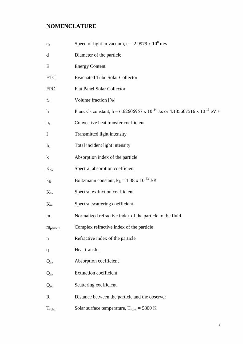
NOMENCLATURE
co Speed of light in vacuum, c = 2.9979 x 10⁸ m/s
d Diameter of the particle
E Energy Content
ETC Evacuated Tube Solar Collector
FPC Flat Panel Solar Collector
fv Volume fraction [%]
h Planck‟s constant, h = 6.62606957 x 10⁻³⁴
J.s or 4.135667516 x 10⁻¹⁵
eV.s
hc Convective heat transfer coefficient
I Transmitted light intensity
Iλ Total incident light intensity
k Absorption index of the particle
Kaλ Spectral absorption coefficient
kB Boltzmann constant, kB = 1.38 x 10⁻²³
J/K
Keλ Spectral extinction coefficient
Ksλ Spectral scattering coefficient
m Normalized refractive index of the particle to the fluid
mparticle Complex refractive index of the particle
n Refractive index of the particle
q Heat transfer
Qaλ Absorption coefficient
Qeλ Extinction coefficient
Qsλ Scattering coefficient
R Distance between the particle and the observer
Tsolar Solar surface temperature, Tsolar = 5800 K

xi
ΔT Temperature difference
v Frequency of photon associated electromagnetic wave
y Length of light path
Greek symbols
α Size parameter
θ Scattering angle
λ Wavelength [μm]

xii
LIST OF APPENDICES
Appendix 1
Calculated Data for Optical Properties of Base Fluid (Pure Water), Nanoparticles
(Aluminium Nanoparticles) and Nanofluid
1
Chapter 1: Introduction
1.0 Background
Fire marked a leap in human civilization history and is used directly or
indirectly in every day‟s life. It is used to cook, sterilize, provide heating during cold
seasons and at night, “landscape management” in agriculture industry in many
developing countries and most importantly, provide thermal energy in power plants to
generate electricity. The hominid fossil record suggests that cooked food may have
appeared as early as 1.9 Ma (Wrangham, et al., 1999) although reliable evidence for
controlled fire use does not appear in the archaeological record until after 400,000 years
ago, with evidence of regular use much later (Karkanas, et al., 2007). The routine
domestic use of fire is believed to begin around 50,000 to 100,000 years ago (Bar-Yosef,
2002).
Conventional electricity generation is an energy conversion process of turning
fire, or more scientifically, heat or thermal energy into kinetic energy by boiling water
to create steam that turns turbines in power plants and eventually turning kinetic energy
into electric energy. The electricity consumed by the world is increasing year by year
and electricity generation has become ever more important to the world. According to
the United States Energy Information Administration, world net electricity generation
increases by an average of 2.3 per cent per year from 2007 to 2035 in the International
Energy Outlook (IEO) 2010 Reference case. Electricity supplies an increasing share of
the world's total energy demand and grows faster than liquid fuels, natural gas, and coal
in all end-use sectors except transportation. From 1990 to 2007, growth in net electricity
generation outpaced the growth in total energy consumption (1.9 per cent per year and
1.3 per cent per year, respectively), and the growth in demand for electricity continues
to outpace growth in total energy use throughout the projection period (U.S. DOE,

2
2010a). This is further illustrated in Figure 1.1 below where net energy generation and
total energy consumption on year 1990 is served as 1.
Figure 1.1 : Growth in world electric power generation and total energy consumption,
1990-2035, Derived from EIA, International Energy Statistics database (as of
November 2009) (U.S. DOE, 2010a)
As the most vastly used and relatively well developed energy system, fossil
fuels can say to be the most vital energy form to human modern civilization. Fossil fuels
such as coal, petroleum and natural gas are used for steam generation in boilers in
electric power plants and these plants stand a majority stack in the electricity power
plant in the whole world. Thousands and millions tons of fossil fuels are burn every day
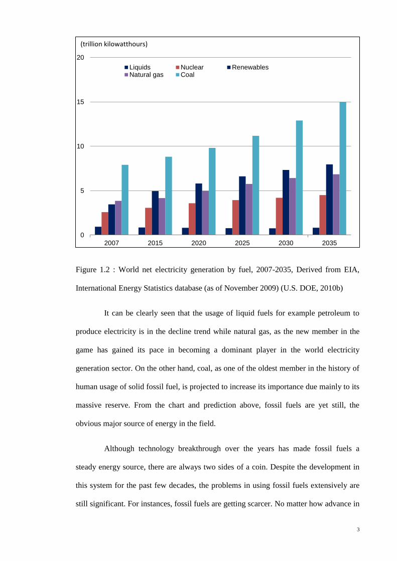
to create enough energy to support human‟s quest for energy. Figure 1.2 shows the
composition of types of fuel used in electricity generation.
0
1
2
3
4
1990 2000 2007 2015 2025 2035
Net electricity generation Total energy consumption(index, 1990 = 1)
3
Figure 1.2 : World net electricity generation by fuel, 2007-2035, Derived from EIA,
International Energy Statistics database (as of November 2009) (U.S. DOE, 2010b)
It can be clearly seen that the usage of liquid fuels for example petroleum to
produce electricity is in the decline trend while natural gas, as the new member in the
game has gained its pace in becoming a dominant player in the world electricity
generation sector. On the other hand, coal, as one of the oldest member in the history of
human usage of solid fossil fuel, is projected to increase its importance due mainly to its
massive reserve. From the chart and prediction above, fossil fuels are yet still, the
obvious major source of energy in the field.
Although technology breakthrough over the years has made fossil fuels a
steady energy source, there are always two sides of a coin. Despite the development in
this system for the past few decades, the problems in using fossil fuels extensively are
still significant. For instances, fossil fuels are getting scarcer. No matter how advance in
0
5
10
15
20
2007 2015 2020 2025 2030 2035
Liquids Nuclear RenewablesNatural gas Coal
(trillion kilowatthours)

4
technology we are in recovering oil wells or digging coal, the truth of using up all fossil
fuels on earth crust one day is inevitable. Production cost is increasing over the years
because of this. Such a scenario is outlined by the Hubbert curve (Tester, et al., 2005),
which projects the production rate of petroleum as a function of time. According to this
projection, it is expected that due to the limited amount of petroleum resources, its rate
of production would peak after a certain amount of time, followed by an increase in its
cost. Moreover the peak is expected to be followed by a sharp drop, which would
provide very little time to develop and switch to alternative technologies once the peak
is reached.
Further to that, air pollution due to burning of fossil fuels has always been a
headache to governments, investors, environmentalists and researchers. Our dependency
on fossil fuels has been damaging our environment irreversibly. Over the past decades,
greenhouse effect has become one of the most talk-about topics relating to energy. As
ozone level depreciating and climate changes are becoming more and more serious, this
issue has to be addressed. The Kyoto Protocol is a protocol to the United Nations
Framework Convention on Climate Change (UNFCCC or FCCC), aimed at combating
global warming. The objective of the Kyoto climate change conference was to establish
a legally binding international agreement, whereby all the participating nations commit
themselves to tackling the issue of global warming and greenhouse gas emissions
(Wikipedia, 2011a). It has been recognized that the carbon dioxide (CO2) is the highest
contributor in the greenhouse effects among the other gases such as sulphur dioxide
(SO2), nitrogen oxide (NOx), and carbon monoxide (CO). CO is colourless and
odourless. Exposure to CO reduces the blood‟s ability to carry oxygen. It might cause
death if one is continuously exposed to high concentration of CO. NOx is a generic term
for mono-nitrogen oxides (NO and NO2). These oxides are produced during combustion,
especially at high temperatures. When NOx and volatile organic compounds (VOCs)

5
react in the presence of sunlight, they form photochemical smog, a significant form of
air pollution, especially in the summer. Children, people with lung diseases such as
asthma, and people who work or exercise outside are susceptible to adverse effects of
smog such as damage to lung tissue and reduction in lung function (US EPA, 2011a).
SO2 is the component of greatest concern and is used as the indicator for the larger
group of gaseous sulphur oxides (SOx). SOx can react with other compounds in the
atmosphere to form small particles. These particles penetrate deeply into sensitive parts
of the lungs and can cause or worsen respiratory disease, such as emphysema and
bronchitis, and can aggravate existing heart disease, leading to increased hospital
admissions and premature death (US EPA, 2011b).
In view the running out of availability, rising cost of production and
environmental impact caused by using fossil fuels to create energy and electricity,
renewable energy is a promising counter measure to the above problems.
1.1 Renewable Energies
Renewable energy can be defined as “energy obtained from the continuous or
repetitive currents of energy recurring in the natural environment” (Twidell and Weir,
2006) or as “energy flows which are replenished at the same rate as they are used”
(Sørenson, 2011). The definitions for renewable energy above both emphasized on
energy “recurring” and “replenishing”, which suggested that this uprising star of energy
sector will not diminish or reduce in its reserve unlike conventional non-renewable
energy. Continuing concerns about the “sustainability” of both fossil fuels and nuclear
energy have been a major spur in bringing renewable energy back into the limelight in
recent decades. By self “recurring” and “replenishing”, renewable energy can tackle all

6
cost related problems from the root as production cost will only become lower when
technologies to harvest this energy are getting more mature.
Renewable energy can also help to reduce poverty through improved basic
energy access like lightings, communications, water pumping, heating and cooling at
some rural areas which are severely underserved with electricity. These will generate
economy growth and gives a start to eliminate extreme poverty. PV household systems,
wind turbines, micro-hydro powered or hybrid mini-grids, biomass-based systems or
solar pumps, and other renewable technologies are being employed in homes, schools,
hospitals, agriculture, and small industry in rural and off-grid areas of the developing
world.
Above and beyond this, one of the key attractiveness of renewable energy is its
environmental friendliness. Despite the fact that renewable energy release close-to-zero
emission when it generates power, there are some arguments saying that the raw
material required for manufacturing of the parts of renewable energy source, such as in
a solar collector, may still lead to some carbon footprint. But however, Masruroh et al.
(2006) demonstrated in a life cycle analysis showing a clear reduction of up to 50% in
carbon footprint by using solar thermal system instead of natural gas or oil for heating
purposes.
Renewable energy consists of Solar Energy, Wind Energy, Wave Energy,
Hydro Energy, Nuclear Energy, Tidal Energy, Geothermal Energy and last but not least
Biomass Energy. Renewable energy, which experienced no downturn in 2009,
continued to grow strongly in all end-use sectors – power, heat and transport – and
supplied an estimated 16% of global final energy consumption (REN21, 2011). These
are further explained with Figure 1.3 and Figure 1.4 below.

7
Figure 1.3 : Renewable energy Share of Global final energy Consumption, 2009 (REN
21, 2011)
Renewable energy accounted for approximately half of the estimated 194
gigawatts (GW) of new electric capacity added globally during the year. Renewables
delivered close to 20% of global electricity supply in 2010, and by early 2011 they
comprised one quarter of global power capacity from all sources. Existing renewable
power capacity worldwide reached an estimated 1,320 gigawatts (GW) in 2010, up
almost 8% from 2009. Renewable capacity now comprises about a quarter of total
global power generating capacity (estimated at 4,950 GW in 2010) and supplies close to
20% of global electricity, with most of this provided by hydropower (REN21, 2011).
This is showed in Figure 1.4 below.
8
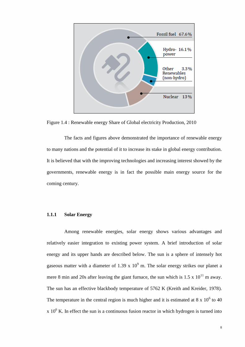
Figure 1.4 : Renewable energy Share of Global electricity Production, 2010
The facts and figures above demonstrated the importance of renewable energy
to many nations and the potential of it to increase its stake in global energy contribution.
It is believed that with the improving technologies and increasing interest showed by the
governments, renewable energy is in fact the possible main energy source for the
coming century.
1.1.1 Solar Energy
Among renewable energies, solar energy shows various advantages and
relatively easier integration to existing power system. A brief introduction of solar
energy and its upper hands are described below. The sun is a sphere of intensely hot
gaseous matter with a diameter of 1.39 x 10⁹ m. The solar energy strikes our planet a
mere 8 min and 20s after leaving the giant furnace, the sun which is 1.5 x 10¹¹
m away.
The sun has an effective blackbody temperature of 5762 K (Kreith and Kreider, 1978).
The temperature in the central region is much higher and it is estimated at 8 x 10⁶ to 40
x 106 K. In effect the sun is a continuous fusion reactor in which hydrogen is turned into

9
helium. The sun‟s total energy output is 3.8 x 10²⁰
MW which is equal to 63 MW/m2 of
the sun‟s surface. This energy radiates outwards in all directions. Only a tiny fraction,
1.7 x 10¹⁴
kW, of the total radiation emitted is intercepted by the earth (Kreith and
Kreider, 1978). However, even with this small fraction it is estimated that 30 min of
solar radiation falling on earth is equal to the world energy demand for one year. Figure
1.5 below illustrates the portion of solar power that are absorbed and reflected by earth,
cloud and atmosphere.
Figure 1.5 : Solar energy distribution (Four Peaks Technologies, 2010)
From Figure 1.5, the average amount of the sun's radiation of 0.70 kilo-watts
per square meter that penetrates the atmosphere and reaches the earth is 51% of the total
incoming energy as illustrated above. Of the 49% that does not reach the earth, 30% is
reflected back into space and 19% is absorbed by the atmosphere and clouds. In 2005,
10
the earth's energy use by mankind was approximately 500 exajoules. This was about
0.01% of the total energy coming from the sun. Putting this in another way, the earth
absorbs more energy in one hour than the world uses in one year according to physicist
Steven Chu, Director of Lawrence Berkeley National Laboratory (Four Peaks
Technologies, 2010). Among the 30% reflected radiant, 4% is reflected by earth‟s
surface which means it can be further reap as well. This means that the total available
portion of solar power to earth to be harvested will equal 55% and most importantly,
this huge source of energy is free and clean to use. All these facts and figures show a
hopeful energy source waiting for mankind to ripe.
As a matter of fact, solar energy is seen to be the highest form of energy by
some researchers. The International Energy Agency (2002) explains: “Renewable
energy is derived from natural processes that are replenished constantly. In its various
forms, it derives directly from the sun, or from heat generated deep within the earth.
Included in the definition is electricity and heat generated from solar, wind, ocean,
hydropower, biomass, geothermal resources, and biofuels and hydrogen derived from
renewable resources”. The above statement gives an idea of two main direct sources of
renewable energies, which are solar power and geothermal power, while other
renewable energies are derivatives of them. In this derivatives form, solar energy goes
through at least one level of energy conversion state. Fossil fuel for example, a form of
energy converted from dead animals compressed in the earth crust millions of years ago,
is another form of solar energy conversion. According to the first law of thermodynamic,
energy cannot be created or destroyed but it may be converted from one form to another.
However, in the second law of thermodynamic, energy conversion might involve
irreversible physical process and the “usable” energy or exergy will decrease. Thus, we
can easily confirm that solar energy is the highest form of energy among renewables
energies. It can be argues that engineers should be able to tailor power generation

11
systems for direct utilization of solar radiation with efficiencies exceeding other multi-
step energy conversion cycles that rely on the earth to modify solar energy into higher
quality and more readily usable energy source.
Solar energy is also a relatively “fair” form of renewable energy. Most
renewable energies are highly geometrically dependent. For instances, wind energy
works well offshore or near shore but weaken abruptly when we move towards inland;
hydro energy needs rivers and dams at preferably higher level to have good potential
energy. While on the other hand, solar energy is best readied near the equator but
through careful system design, it is available even in winter of seasonal countries.
Interest in solar energy has prompted the accurate measurement and mapping of solar
energy resources over the globe. The yearly sum of global irradiance is displayed in
Figure 1.6 below. It can be seen that most part of the earth receive more or less the same
total amount of radiant per annum. Solar power gradually decrease with greater latitude
but in most developed nations, the power exposed is still promising.
Figure 1.6 : Yearly sum of global irradiance (Meteonorm, 2008)
12
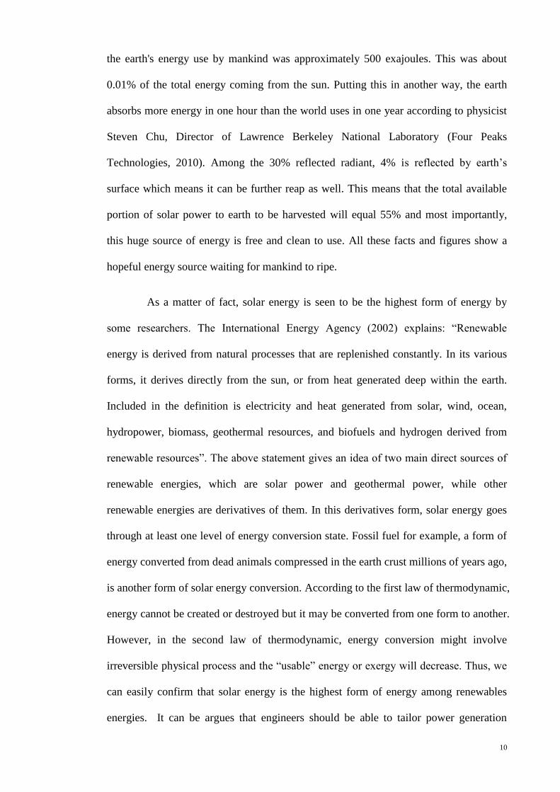
This is normally done using solarimeters as illustrated in Figure 1.7. These
contain carefully calibrated thermoelectric elements fitted under a glass cover, which is
open to the whole vault of the sky. A voltage proportional to the total incident light
energy is produced and then recorded electronically (Everett, 2004)
Figure 1.7 : A Solarimeter, also refer to as a “Pyranometer”
With the higher energy form and availability of solar power, it is favoured to
researchers in further developing it. Nonetheless, certain limits on the efficiency of
direct solar power generation exist; current solar thermal technologies are not
functioning close to these limits which leave room for enhancement for future solar
thermal systems. The efficiency of a solar thermal collector relies on the effectiveness
of absorbing solar radiant power and heat transfer from the absorber to the carrier,
which is normally fluid. The conversion of highly concentrated sunlight into thermal
energy suffers from relatively low efficiencies of 50% to 60% (Pacheco, 2001).
Furthermore, current solar thermal power plants offer limited energy storage in order to
13
buffer the diurnal nature of the solar radiation. The overall efficiency of generating
power in these plants is approximately 15% (Pacheco, 2001), whereas fossil power
plants have reached efficiencies exceeding 50% in combined cycle plants. By way of
higher improving the receivers and heat transfer mechanisms, direct solar collector can
work closer to its limit. This thesis contributes in making solar thermal power
generation more ubiquitous in the future.
1.2 Objective
The objectives of this thesis are the following:
1. To investigate the suitability of nanofluid to be used as a volumetric absorber.
2. To explore the radiative properties of the two components of nanofluid, namely
the base fluid and the nanoparticles.
3. To propose nanoparticle sizes and volume fractions for nanofluid.
4. To compares the transmissivity of light through base fluid and nanofluid.
1.3 Thesis Organization
This thesis begins with the introduction to the current energy crisis, the
environmental issues faced and the possible of overcoming them by utilizing renewable
energy. Chapter 2 includes the literature reviews that describe the basic light properties
and equations, the working principles of solar collector, particularly Flat Plate Solar
Collector (FPC) and Evacuated Tube Solar Collector (ETC) and the current studies of
nanofluid in terms of optical properties and the proposal of using it as volumetric
absorber. FPC and ETC are introduced these two types of collectors have similar
14
working principle with Direct Absorption Solar Collector (DAC). With the change of
working fluid to nanofluid as volumetric absorber, FPC and ETC will become a DAC.
Chapter 3 discusses the methodology of this thesis. The governing equations to
calculate the optical properties of base fluid and nanoparticles are discussed in detail in
this chapter. The results obtained with the equations and the discussions are presented in
Chapter 4 while the last chapter, Chapter 5, concludes the study and gives future
recommendations to the researchers.
15
Chapter 2: Literature Review
2.0 Introduction
The literature review for this thesis will includes mainly three parts. In the first
part, the properties of light and some important terminologies are discussed. The second
section will give description to solar collector and the last section will review the
current studies of nanofluid in terms of optical properties and the incorporation into
solar collectors.
2.1 Properties of Light
Before the description of solar collectors, it is crucial that the basic or primary
properties of light and some key terminology are explained to give a better
understanding to the further part of the discussion.
Light or visible light is electromagnetic radiation that is visible to the human
eye, and is responsible for the sense of sight. Everything we see and the beautiful
colours from the blue sky and green mountains are merely the reflection and scattering
of light. Visible light has wavelength in a range from about 380 nanometres to about
740 nm, with a frequency range of about 405 THz to 790 THz. The visible range
extends from the extreme violet at about 400 nm to the extreme red at about 700 nm
according to Smith (2006). From short to long wavelengths, the colours across the
visible spectrum are: violet, indigo, blue, cyan (blue-green), green, yellow, orange and
red. Figure 2.1 below shows light spectrum with their respective wavelength while table
2.1 gives more detail to each specific colour and its particular range of frequency and
wavelength.
16
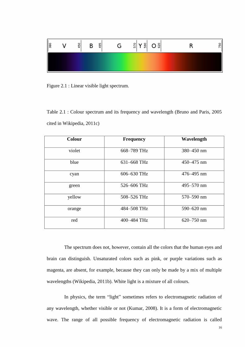
Figure 2.1 : Linear visible light spectrum.
Table 2.1 : Colour spectrum and its frequency and wavelength (Bruno and Paris, 2005
cited in Wikipedia, 2011c)
Colour Frequency Wavelength
violet 668–789 THz 380–450 nm
blue 631–668 THz 450–475 nm
cyan 606–630 THz 476–495 nm
green 526–606 THz 495–570 nm
yellow 508–526 THz 570–590 nm
orange 484–508 THz 590–620 nm
red 400–484 THz 620–750 nm
The spectrum does not, however, contain all the colors that the human eyes and
brain can distinguish. Unsaturated colors such as pink, or purple variations such as
magenta, are absent, for example, because they can only be made by a mix of multiple
wavelengths (Wikipedia, 2011b). White light is a mixture of all colours.
In physics, the term “light” sometimes refers to electromagnetic radiation of
any wavelength, whether visible or not (Kumar, 2008). It is a form of electromagnetic
wave. The range of all possible frequency of electromagnetic radiation is called

17
electromagnetic spectrum. The electromagnetic spectrum extends from low frequencies
used for modern radio to gamma radiation at the short-wavelength end, covering
wavelengths from thousands of kilometers down to a fraction of the size of an atom.
The long wavelength limit is the size of the universe itself, while it is thought that the
short wavelength limit is in the vicinity of the Planck length, although in principle the
spectrum is infinite and continuous. Based on a figure from NASA, figure 2.2 illustrates
the relationship between the wavelength and frequency of electromagnetic wave and
also gives an idea to the scale of the wavelength. Some radiations are marked as "N" for
"no" in the diagram to show that they cannot penetrate the atmosphere, although
extremely minimally of such radiations do still penetrate the atmosphere.
Figure 2.2 : Electromagnetic spectrum
In electromagnetic (EM) wave, the wavelength is inversely proportional to the
frequency. Gamma ray may have the shortest wavelength but it has the highest
frequency in EM wave. The relationship between energy content and frequency of EM
wave is called the Planck relation or the Planck–Einstein equation:
18
(2.1)
where h is the Planck‟s constant and is equal to 6.62606957 x 10⁻³⁴
J.s or 4.135667516
x 10-15
eV.s (Mohr, et al., 2011) and v is the frequency of photon associated
electromagnetic wave and is related to speed of light in vacuum, co, by λv = co. This
gives the Planck relation to become:
(2.2)
This relation demonstrates that the wavelength is inversely proportional to energy. As
so, gamma ray has the highest energy while radio wave has the lowest.
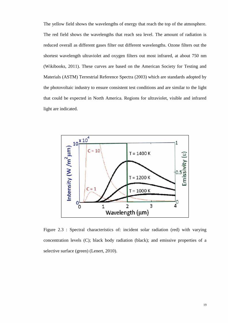
Although EM wave has higher energy when the wavelength is shorter, the solar
radiation has a characteristic peak at a wavelength of 500 nm and approximately 95% of
its overall power below 2,000 nm (Lenert, 2010). Figure 2.3 shows the spectral
distribution of the incident solar radiation as approximated by a black body spectrum at
a temperature of 5787 K (illustrated in red). As the solar radiation is concentrated, the
intensity scales with the concentration level (C). An ideal receiver will absorb the
concentrated solar radiation, convert that incident solar radiation into heat and transfer
the heat to the heat transfer fluid.
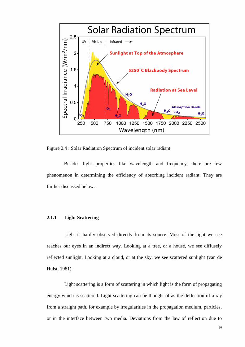
Figure 2.4 displays the solar radiation spectrum for direct light at both the top
of the Earth's atmosphere and at sea level. The sun produces light with a distribution
similar to what would be expected from a 5525 K (5250 °C) blackbody, which is
approximately the sun's surface temperature. As light passes through the atmosphere,
some is absorbed by gases with specific absorption bands. Additional light is
redistributed by Rayleigh scattering, which is responsible for the atmosphere's blue
color. In the atmosphere, gases filter some wavelengths from incoming solar energy.
19
The yellow field shows the wavelengths of energy that reach the top of the atmosphere.
The red field shows the wavelengths that reach sea level. The amount of radiation is
reduced overall as different gases filter out different wavelengths. Ozone filters out the
shortest wavelength ultraviolet and oxygen filters out most infrared, at about 750 nm
(Wikibooks, 2011). These curves are based on the American Society for Testing and
Materials (ASTM) Terrestrial Reference Spectra (2003) which are standards adopted by
the photovoltaic industry to ensure consistent test conditions and are similar to the light
that could be expected in North America. Regions for ultraviolet, visible and infrared
light are indicated.
Figure 2.3 : Spectral characteristics of: incident solar radiation (red) with varying
concentration levels (C); black body radiation (black); and emissive properties of a
selective surface (green) (Lenert, 2010).
20
Figure 2.4 : Solar Radiation Spectrum of incident solar radiant
Besides light properties like wavelength and frequency, there are few
phenomenon in determining the efficiency of absorbing incident radiant. They are
further discussed below.
2.1.1 Light Scattering
Light is hardly observed directly from its source. Most of the light we see
reaches our eyes in an indirect way. Looking at a tree, or a house, we see diffusely
reflected sunlight. Looking at a cloud, or at the sky, we see scattered sunlight (van de
Hulst, 1981).
Light scattering is a form of scattering in which light is the form of propagating
energy which is scattered. Light scattering can be thought of as the deflection of a ray
from a straight path, for example by irregularities in the propagation medium, particles,
or in the interface between two media. Deviations from the law of reflection due to

21
irregularities on a surface are also usually considered to be a form of scattering
(Wikipedia, 2011d). Most objects that one sees are visible due to light scattering from
their surfaces. Indeed, this is our primary mechanism of physical observation (Kerker,
1909 cited in Wikipedia, 2011d; Mandelstam, 1926, cited in Wikipedia, 2011d).
Scattering of light depends on the wavelength or frequency of the light being scattered.
Since visible light has wavelength on the order of a micron, objects much smaller than
this cannot be seen, even with the aid of a microscope. Colloidal particles as small as 1
µm have been observed directly in aqueous suspension (van de Hulst, 1981)
Light will not scatter when it traverses across homogeneous medium. In fact,
any material medium has inhomogeneity as it consists of molecules, each of which acts
as a scattering center, but it depends on the arrangement of these molecules whether the
scattering will be very effective. In a perfect crystal at zero absolute temperature, the
molecules are arranged in a very regular way, and the waves scattered by each molecule
interfere in such a way as to cause no scattering at all but just a change in the overall
velocity of propagation (van de Hulst, 1981). In a gas, or fluid, on the other hand,
statistical fluctuations in the arrangement of the molecules cause a real scattering,
sometimes may be appreciable, which in this study, will be refer to the study of
nanofluid.
There are a handful types of light scattering phenomenon discovered or
explained so far by scientists, for instance Mie scattering, Rayleigh scattering, Raman
scattering, Tyndall scattering and Brillouin scattering. Among these, Rayleigh scattering
and Mie scattering are the two most commonly used and important theories to explain
the light scattering phenomenon.
22
2.1.1.1 Rayleigh Scattering
Rayleigh scattering, named after the British physicist Lord Rayleigh, is defined
by a mathematical formula that requires the light-scattering particles to be far smaller
than the wavelength of the light. For a dispersion of particles to qualify for the Rayleigh
formula, the particle sizes need to be below roughly 40 nanometers; and the particles
may be individual molecules. Rayleigh scattering gives blue scattered light and explains
the origin of the blue sky in 1899 (Rayleigh and Strutt, 1909 cited in Horvath, 2009,
p.790; Lilienfeld, 2004). In Rayleigh scattering, the intensity of the scattered radiation is
given by:
(
)
(
)
(
)
(2.3)
where R is the distance between the particle and the observer,
θ is the scattering angle,
n is the refractive index of the particle, and
d is the diameter of the particle.
It can be seen from the above equation that Rayleigh scattering is strongly
dependent upon the size of the particle and the wavelengths. The intensity of the
Rayleigh scattered radiation increases rapidly as the ratio of particle size to wavelength
increases. The Rayleigh scattering model breaks down when the particle size becomes
larger than around 10% of the wavelength of the incident radiation. In the case of
particles with dimensions greater than this, Mie's scattering model can be used to find
23
the intensity of the scattered radiation. Thus, scattering by particles similar to or larger
than the wavelength of light is typically treated by the Mie theory.
2.1.1.2 Mie Scattering
Mie scattering or Mie theory was named after German professor of physics
Gustav Mie (1868 – 1957). His work was a rigorous treatment of the interaction of light
with a particle smaller than or comparable to the wavelength of light and combined
theory with applications to a real practical case: the scattering and absorption of light,
its polarization, and colour phenomena observed for gold colloids (Horvath, 2009).
Mie scattering can use to calculate the spectrum of the scattered light. For
particles with sizes between 20 and 140 nm, almost independently of size, the scattered
light is green to yellow, the largest amount of light is scattered by particles sized
between 100 and 140 nm. Particles with sizes between 140 and 180 nm predominantly
scatter orange to red light. Both theoretical findings are in agreement with observations
(Horvath, 2009).
Mie scattering also explains the polarization of light particles. It is stated that if
particles are illuminated by unpolarized light, the scattered light is usually partly
polarized. For particles smaller than 100 nm (Rayleigh scattering) the light scattered at
90º is completely polarized, which is also true for gold particles. For particles with sizes
between 100 and 180 nm the degree of polarization diminishes rapidly with increasing
particle size, again in agreement with the observations (Horvath, 2009). Three diagrams
taken from Mie‟s publication are shown in Figure 2.5 for a wavelength of 550 nm.
24
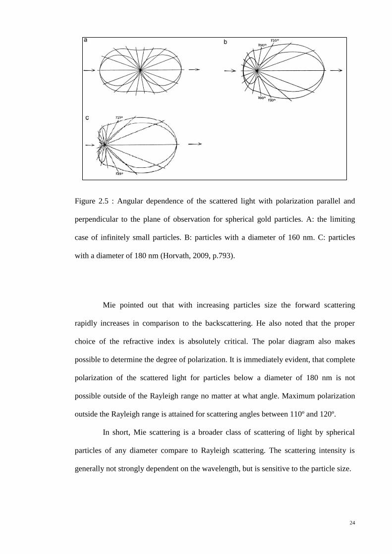
Figure 2.5 : Angular dependence of the scattered light with polarization parallel and
perpendicular to the plane of observation for spherical gold particles. A: the limiting
case of infinitely small particles. B: particles with a diameter of 160 nm. C: particles
with a diameter of 180 nm (Horvath, 2009, p.793).
Mie pointed out that with increasing particles size the forward scattering
rapidly increases in comparison to the backscattering. He also noted that the proper
choice of the refractive index is absolutely critical. The polar diagram also makes
possible to determine the degree of polarization. It is immediately evident, that complete
polarization of the scattered light for particles below a diameter of 180 nm is not
possible outside of the Rayleigh range no matter at what angle. Maximum polarization
outside the Rayleigh range is attained for scattering angles between 110º and 120º.
In short, Mie scattering is a broader class of scattering of light by spherical
particles of any diameter compare to Rayleigh scattering. The scattering intensity is
generally not strongly dependent on the wavelength, but is sensitive to the particle size.
25
2.1.2 Light Absorption
Scattering is often accompanied by absorption. A leaf of a tree looks green
because it scatters green light more effectively than red light. The red light incident on
the leaf is absorbed; this means that its energy is converted into some other form and is
no longer present as red light. Absorption is preponderant in materials such as coal and
black smoke and is nearly absent in clouds (van de Hulst, 1981). Figure 2.6 below
illustrates the process of light absorption and the change of energy of particles when
absorption happens.
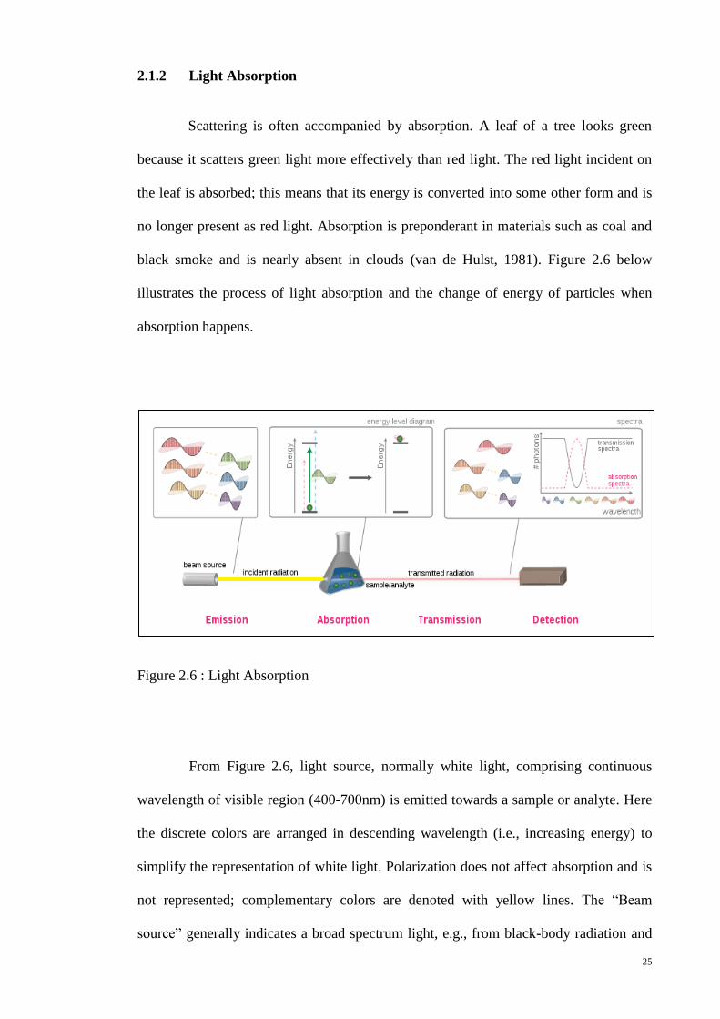
Figure 2.6 : Light Absorption
From Figure 2.6, light source, normally white light, comprising continuous
wavelength of visible region (400-700nm) is emitted towards a sample or analyte. Here
the discrete colors are arranged in descending wavelength (i.e., increasing energy) to
simplify the representation of white light. Polarization does not affect absorption and is
not represented; complementary colors are denoted with yellow lines. The “Beam
source” generally indicates a broad spectrum light, e.g., from black-body radiation and
26
laser beam is not within this scope as they are monochromatic (single wavelength).
Light in the visible region induces electronic excitation and it will rearrange the electron
clouds. This applies only for visible light - the removal of a colour results in beam
appearing as its complementary color. Here, the removal of green within the red-green
pair gives the transmitted beam a red color when light beam traverses through the
sample. Molecules have quantized energy levels, and photons have quantized energy. If
the incoming photon has exactly the matching energy for the promotion of the molecule,
the molecule would absorb the photon, and changes state from the ground state to an
excited state. The specific physical change depends on the radiation. A spectra is
effectively a continuous histogram describing the composition of light. By comparing
the attenuation of the transmitted light with the incident, absorption spectra can be
obtained. Absorption spectra is represented as a transmission spectra, which is shown in
gray in Figure 2.5, where the y-axis shows the photon count of transmitted light, or an
absorption spectra (magenta) where the attenuation is plotted. The former is commonly
used in infrared/microwave spectroscopy, and the latter in UV-Vis and NMR.
2.1.3 Light Extinction
Both scattering and absorption remove energy from a beam of light traversing
the medium. The beam is then attenuated. This attenuation, which is called extinction, is
seen when we look directly at the light source. The sun, for instance, is fainter and
redder at the sunset than at noon. This indicates extinction in the long air path, which is
strong in all colours but even stronger in blue light than in red light. Extinction can be
defines as scattering plus absorption (van de Hulst, 1981).
27
(2.4)
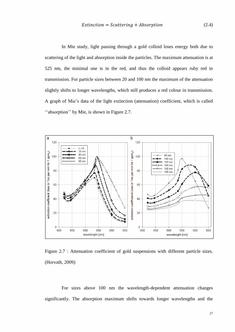
In Mie study, light passing through a gold colloid loses energy both due to
scattering of the light and absorption inside the particles. The maximum attenuation is at
525 nm, the minimal one is in the red, and thus the colloid appears ruby red in
transmission. For particle sizes between 20 and 100 nm the maximum of the attenuation
slightly shifts to longer wavelengths, which still produces a red colour in transmission.
A graph of Mie‟s data of the light extinction (attenuation) coefficient, which is called
„„absorption‟‟ by Mie, is shown in Figure 2.7.
Figure 2.7 : Attenuation coefficient of gold suspensions with different particle sizes.
(Horvath, 2009)
For sizes above 100 nm the wavelength-dependent attenuation changes
significantly. The absorption maximum shifts towards longer wavelengths and the

28
weakest attenuation is between 400 and 450 nm, causing the colloid to appear violet in
transmission for particle sizes ~100nm, deep blue for ~120 nm, indigo for ~160 nm, and
green–blue for ~180 nm. These results give an important guide in choosing the size of
nanoparticles to be used in nanofluid for Direct Solar Absorber. The nanoparticles size
is suggested to be smaller than 100 nm as the solar radiant has peak concentration
around the wavelength of 500 nm (Lenert, 2010) as discussed in section 2.1.
2.2 Solar Collectors
As explained in the previous chapter, solar energy can perceive to be a higher
level of energy. Basically, all the forms of energy in the world as we know it are solar in
origin. Oil, coal, natural gas and woods were originally produced by photosynthetic
processes, followed by complex chemical reactions in which decaying vegetation was
subjected to very high temperatures and pressures over a long period of time (Kreith and
Kreider, 1978). Even the wind and tide energy have a solar origin since they are caused
by differences in temperature in various regions of the earth. In such, harvesting energy
directly from solar can avoid losses in the process of converting energy from one form
to the other. Besides, the lesser processes or steps it is to convert solar energy into
electrical power or any usable energy form to us may help to reduce carbon footprint.
The idea of using solar energy collectors to harness the sun‟s power is recorded
from the prehistoric times when at 212 BC the Greek scientist/physician Archimedes
devised a method to burn the Roman fleet. Archimedes reputedly set the attacking
Roman fleet afire by means of concave metallic mirror in the form of hundreds of
polished shields; all reflecting on the same ship (Anderson, 1977). There were many
developments in methods of solar harvesting ever since Archimedes (Meinel and
Meinel, 1976; Kreider and Kreith, 1977).
29
In water and space heating sector, the hot water and house heating appeared in
the mid-1930s, but gained interest in the last half of the 40s. Until then millions of
houses were heated by coal burn boilers. The idea was to heat water and fed it to the
radiator system that was already installed (Kalogirou, 2004). Currently in freezing
climates, solar water heating costs US$0.11–0.12/kWh, while in mild or “sunbelt”
climates, solar water heating costs about US$0.08–0.10/kWh. In some countries such as
China, solar water heating systems are already competitive with conventional systems
in certain climates (EGRE, 2005).
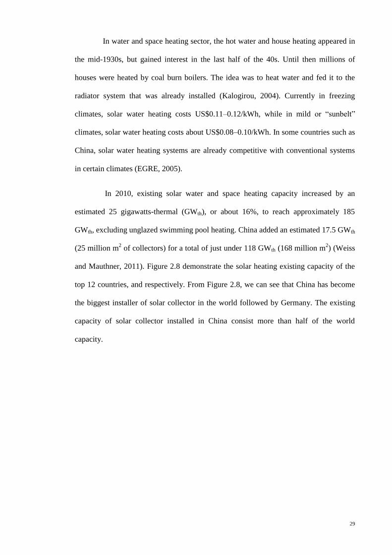
In 2010, existing solar water and space heating capacity increased by an
estimated 25 gigawatts-thermal (GWth), or about 16%, to reach approximately 185
GWth, excluding unglazed swimming pool heating. China added an estimated 17.5 GWth
(25 million m2 of collectors) for a total of just under 118 GWth (168 million m
2) (Weiss
and Mauthner, 2011). Figure 2.8 demonstrate the solar heating existing capacity of the
top 12 countries, and respectively. From Figure 2.8, we can see that China has become
the biggest installer of solar collector in the world followed by Germany. The existing
capacity of solar collector installed in China consist more than half of the world
capacity.

30
Figure 2.8 : Solar heating existing Capacity, Top 12 Countries, 2009 (Weiss and
Mauthner, 2011)
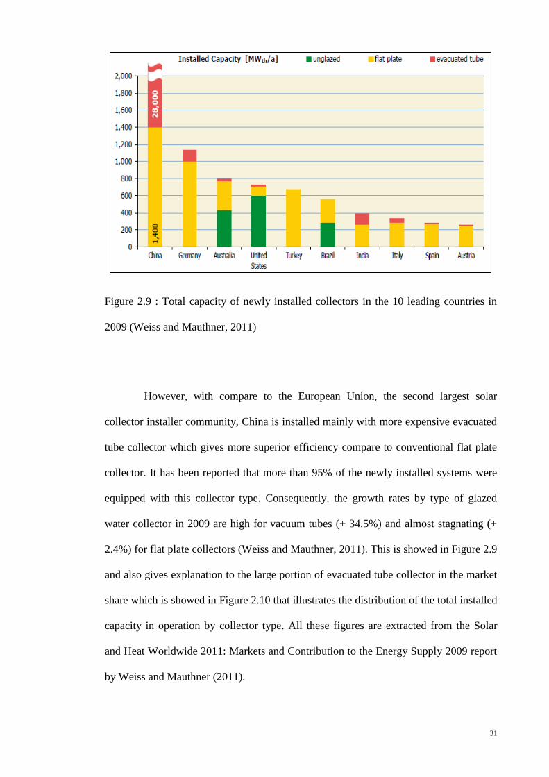
Besides having the most solar collectors installed, figure 2.9 which shows the
total capacity of newly installed glazed and unglazed water collectors in the 10 leading
countries also indicates that China is growing in the fastest pace in 2009 as the
European Union and major western markets had been hit hard by economy meltdown.
The leading market in Europe, Germany, underwent a downturn of 23.1% in its newly
installed capacity of glazed water collectors compared with 2008 (Weiss and Mauthner,
2011). In general, market development had been affected by lower fossil fuel prices and
declining end-user investments.
31
Figure 2.9 : Total capacity of newly installed collectors in the 10 leading countries in
2009 (Weiss and Mauthner, 2011)
However, with compare to the European Union, the second largest solar
collector installer community, China is installed mainly with more expensive evacuated
tube collector which gives more superior efficiency compare to conventional flat plate
collector. It has been reported that more than 95% of the newly installed systems were
equipped with this collector type. Consequently, the growth rates by type of glazed
water collector in 2009 are high for vacuum tubes (+ 34.5%) and almost stagnating (+
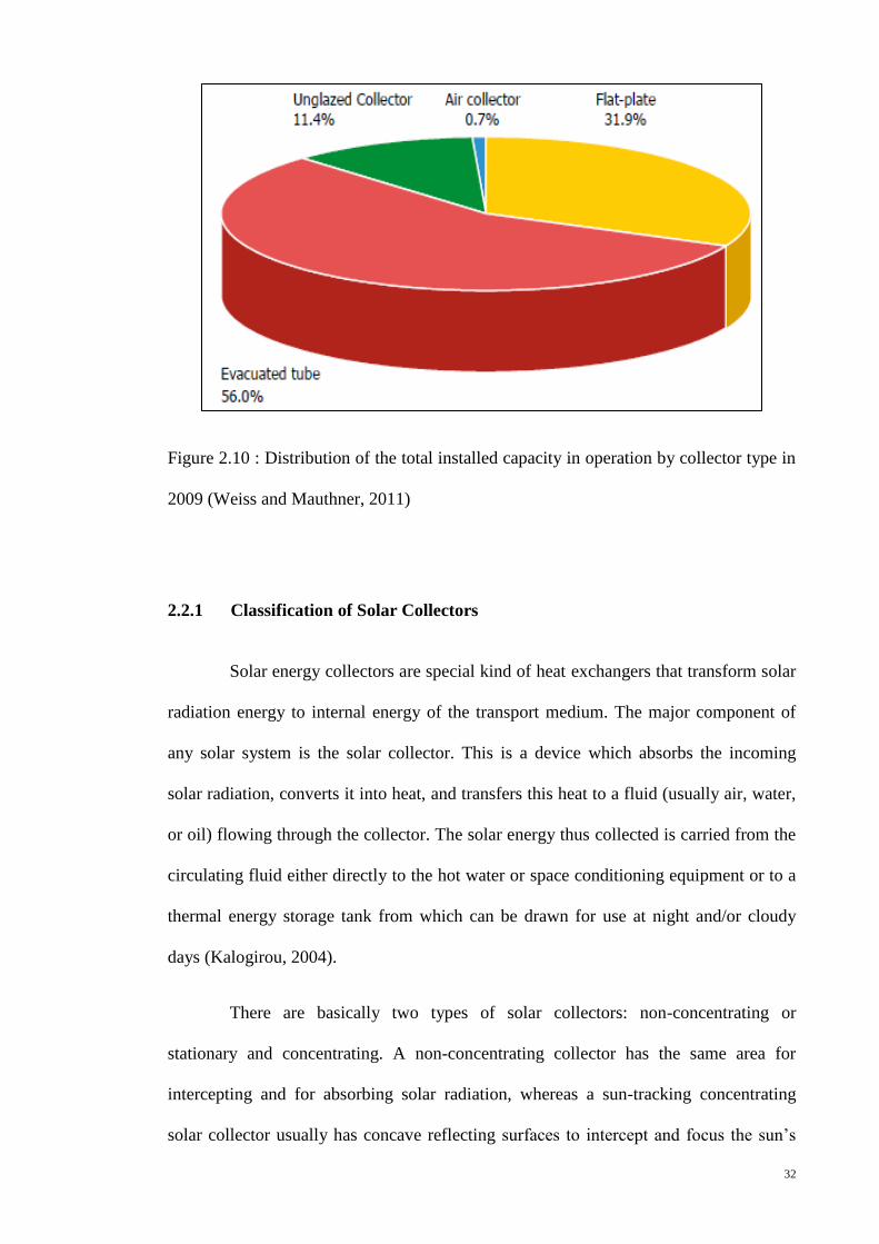
2.4%) for flat plate collectors (Weiss and Mauthner, 2011). This is showed in Figure 2.9
and also gives explanation to the large portion of evacuated tube collector in the market
share which is showed in Figure 2.10 that illustrates the distribution of the total installed
capacity in operation by collector type. All these figures are extracted from the Solar
and Heat Worldwide 2011: Markets and Contribution to the Energy Supply 2009 report
by Weiss and Mauthner (2011).
32
Figure 2.10 : Distribution of the total installed capacity in operation by collector type in
2009 (Weiss and Mauthner, 2011)
2.2.1 Classification of Solar Collectors
Solar energy collectors are special kind of heat exchangers that transform solar
radiation energy to internal energy of the transport medium. The major component of
any solar system is the solar collector. This is a device which absorbs the incoming
solar radiation, converts it into heat, and transfers this heat to a fluid (usually air, water,
or oil) flowing through the collector. The solar energy thus collected is carried from the
circulating fluid either directly to the hot water or space conditioning equipment or to a
thermal energy storage tank from which can be drawn for use at night and/or cloudy
days (Kalogirou, 2004).
There are basically two types of solar collectors: non-concentrating or
stationary and concentrating. A non-concentrating collector has the same area for
intercepting and for absorbing solar radiation, whereas a sun-tracking concentrating
solar collector usually has concave reflecting surfaces to intercept and focus the sun‟s

33
beam radiation to a smaller receiving area, thereby increasing the radiation flux
(Kalogirou, 2003). During the past 50 years many variations were designed and
constructed using focusing collectors as a means of heating the transfer or working fluid
which powered mechanical equipment. With such, a large number of solar collectors are
available in the market. A comprehensive list is shown in Table 2.2.
Table 2.2 : Types of solar energy collectors (Kalogirou, 2003)
Motion Collector type Absorber type
Concentration
ratio
Indicative
temperature
range (ºC)
Stationary
Flat plate collector
(FPC)
Flat 1 30 – 80
Evacuated tube
collector (ETC)
Flat 1 50 – 200
Compound
parabolic collector
(CPC)
Tubular 1 – 5 60 – 240
Single-
axis
tracking
5 – 15 60 – 300
Linear Fresnel
reflector (LFR)
Tubular 10 – 40 60 – 250
Parabolic trough
collector (PTC)
Tubular 15 – 45 60 – 300
Cylindrical trough
collector (CTC)
Tubular 10 – 50 60 – 300
34
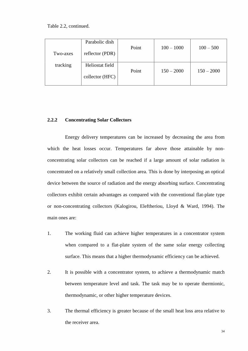
Table 2.2, continued.
Two-axes
tracking
Parabolic dish
reflector (PDR)
Point 100 – 1000 100 – 500
Heliostat field
collector (HFC)
Point 150 – 2000 150 – 2000
2.2.2 Concentrating Solar Collectors
Energy delivery temperatures can be increased by decreasing the area from
which the heat losses occur. Temperatures far above those attainable by non-
concentrating solar collectors can be reached if a large amount of solar radiation is
concentrated on a relatively small collection area. This is done by interposing an optical
device between the source of radiation and the energy absorbing surface. Concentrating
collectors exhibit certain advantages as compared with the conventional flat-plate type
or non-concentrating collectors (Kalogirou, Eleftheriou, Lloyd & Ward, 1994). The
main ones are:
1. The working fluid can achieve higher temperatures in a concentrator system
when compared to a flat-plate system of the same solar energy collecting
surface. This means that a higher thermodynamic efficiency can be achieved.
2. It is possible with a concentrator system, to achieve a thermodynamic match
between temperature level and task. The task may be to operate thermionic,
thermodynamic, or other higher temperature devices.
3. The thermal efficiency is greater because of the small heat loss area relative to
the receiver area.
35
4. Reflecting surfaces require less material and are structurally simpler than FPC.
For a concentrating collector the cost per unit area of the solar collecting
surface is therefore less than that of a FPC.
5. Owing to the relatively small area of receiver per unit of collected solar energy,
selective surface treatment and vacuum insulation to reduce heat losses and
improve the collector efficiency are economically viable.
Their disadvantages are:
1. Concentrator systems collect little diffuse radiation depending on the
concentration ratio.
2. Some form of tracking system is required so as to enable the collector to follow
the sun.
3. Solar reflecting surfaces may lose their reflectance with time and may require
periodic cleaning and refurbishing.
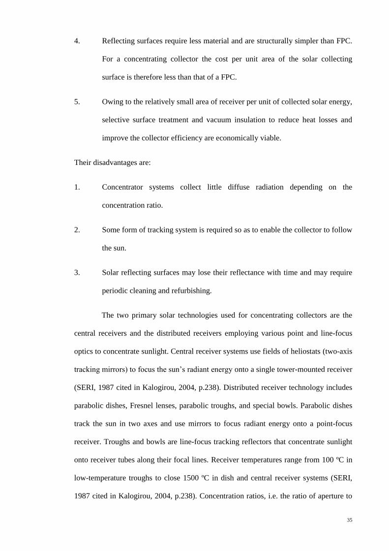
The two primary solar technologies used for concentrating collectors are the
central receivers and the distributed receivers employing various point and line-focus
optics to concentrate sunlight. Central receiver systems use fields of heliostats (two-axis
tracking mirrors) to focus the sun‟s radiant energy onto a single tower-mounted receiver
(SERI, 1987 cited in Kalogirou, 2004, p.238). Distributed receiver technology includes
parabolic dishes, Fresnel lenses, parabolic troughs, and special bowls. Parabolic dishes
track the sun in two axes and use mirrors to focus radiant energy onto a point-focus
receiver. Troughs and bowls are line-focus tracking reflectors that concentrate sunlight
onto receiver tubes along their focal lines. Receiver temperatures range from 100 ºC in
low-temperature troughs to close 1500 ºC in dish and central receiver systems (SERI,
1987 cited in Kalogirou, 2004, p.238). Concentration ratios, i.e. the ratio of aperture to
36
absorber areas, can vary over several orders of magnitude, from as low as unity to high
values of the order of 10,000 (Kalogirou, 2004). Obviously, increased ratios mean
increased temperatures at which energy can be delivered but consequently these
collectors have increased requirements for precision in optical quality and positioning of
the optical system. Figure 2.11 gives a clearer illustration to the above mentioned solar
collectors.
Figure 2.11 : Concentration of sunlight using (a) parabolic trough collector (b) linear
Fresnel collector (c) central receiver system with dish collector and (d) central receiver
system with distributed reflectors

37
2.2.3 Non-Concentrating Solar Collectors
For non-concentrating collectors, hot water heating system is an important field
as mentioned in the previous section. The hot water heating system uses mainly
stationary solar collector which are permanently fixed in position and do not track the
sun. These collectors consist of flat plate collector (FPC) (glazed or unglazed),
evacuated tube collector (ETC) and stationary compound parabolic collector (CPC).
The passive thermosiphon system is the most common type of solar water heating
system worldwide. Simple flat plate collectors made of copper absorbers, aluminum
enclosures, and glass cover plates were the predominant technology for this system for
the last few decades (EGRE, 2005). However, evacuated tube collectors have recently
dominated the world market because of the development of water-in-glass evacuated
tube systems in China.
Being the major market player and also the system in which the effect of
nanofluid as thermal transfer fluid is studied in this thesis, the flat plate collector and
evacuated tube collector are briefly discussed and elucidated.
2.2.3.1 Flat Plate Solar Collector (FPC)
The most commonly used systems in water heating system are the flat-plate,
black-surface absorbers, which absorb solar energy through a solid surface (Okujagu &
Adjepong 1989). Figure 2.12 below shows a typical flat plate collector set up used in
water heating. The solar collector is installed at the roof of the building with certain
designed tilt angle to maximize the incident solar radiant. A close loop circuit with
water or heat transfer fluid flows through the solar collector with the help of a pump.
The fluid is heated up when it passes by the collector and the heat is ejected or released

38
to a water storage tank. The water in the storage tank is now heated and ready to be used.
A boiler, either gas or electric powered, is normally supplied in the system to serve as a
standby power source in the time of insufficient solar energy.
Figure 2.12 : Typical set up of Flat Plate Collector (FPC)
Besides this set up, there is another similar arrangement commonly used in the
market called Thermosyphon solar water heater. Figure 2.13 below displays this type of
arrangement.

39
Figure 2.13 : Thermosyphon Solar water heater
Thermosyphon solar water heater works with exactly the same concept and
pattern as the typical set up except it does not have a pump installed in the system. The
advantage of this arrangement is that it can save space and cost by omitting the pump.
The need of maintenance to the system become close to nil as there is basically no
moving parts. These advantages make it a more favourable system in today‟s property
development as living space has become a major limitation in big cities. However, this
system has its restriction. The water tank has to be located above the solar collector
within certain height and distance (about 30cm) to allow the heat transfer fluid to flow
naturally from the collector to the water tank with the help of natural convection and to
prevent backflow of cooler storage water to the collector in the case when the collector
is colder than the water stored. The water in the collector expands becoming less dense
as the sun heats it and rises through the collector into the top of the storage tank. There
it is replaced by the cooler water that has sunk to the bottom of the tank, from which it
flows down the collector. At night, or whenever the collector is cooler than the water in
the tank the direction of the thermosyphon flow will reverse, thus cooling the stored
water.

40
Disregard of which system been used, the flat plate solar collector is the same.
FPC has been built in a wide variety of designs and from many different materials. They
have been used to heat fluids such as water, water plus antifreeze additive, or air. Their
major purpose is to collect as much solar energy as possible at the lower possible total
cost. The collector should also have a long effective life, despite the adverse effects of
the sun‟s ultraviolet radiation, corrosion and clogging because of acidity, alkalinity or
hardness of the heat transfer fluid, freezing of water, or deposition of dust or moisture
on the glazing, and breakage of the glazing because of thermal expansion, hail,
vandalism or other causes. These causes can be minimized by the use of tempered glass.
A typical flat plate solar collector is shown in figure 2.14 and 2.15 in pictorial and
exploded view respectively.
Figure 2.14 : Pictorial view of a flat plate collector (Kalogirou, 2004, p.241)

41
Figure 2.15 : Exploded view of a flat plate collector (Kalogirou, 2004, p.241)
When solar radiation passes through a transparent cover and impinges on the
blackened absorber surface of high absorptivity, a large portion of this energy is
absorbed by the plate and then transferred to the transport medium in the fluid tubes to
be carried away for storage or use. The underside of the absorber plate and the side of
casing are well insulated to reduce conduction losses. The liquid tubes can be welded to
the absorbing plate, or they can be an integral part of the plate. The liquid tubes are
connected at both ends by large diameter header tubes. The transparent cover is used to
reduce convection losses from the absorber plate through the restraint of the stagnant air
layer between the absorber plate and the glass. It also reduces radiation losses from the
collector as the glass is transparent to the short wave radiation received by the sun but it
is nearly opaque to long-wave thermal radiation emitted by the absorber plate
(greenhouse effect).
Every part shown in the figures above has its own function. The glazing may
have one or more sheets of glass or other diathermanous material for light transmitting.
42
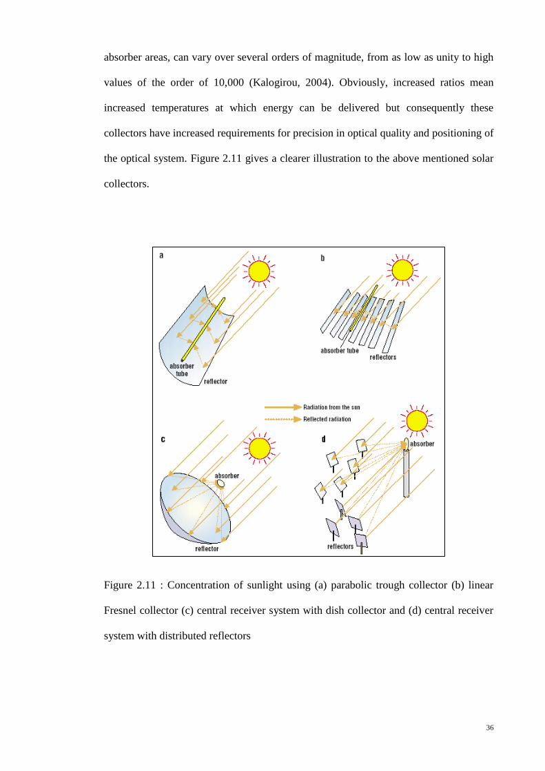
The glazing should admit as much solar irradiation as possible and reduce the upward
loss of heat as much as possible. Table 2.3 below shows the optical properties of
commonly used glazing materials. The solar transmittance is high (close to 1.0) while
the long-wave infra-red transmittance is very low by comparison (Everett, 2004).
Although glass is virtually opaque to the long wave radiation emitted by collector plates,
absorption of that radiation causes an increase in the glass temperature and a loss of heat
to the surrounding atmosphere by radiation and convection.
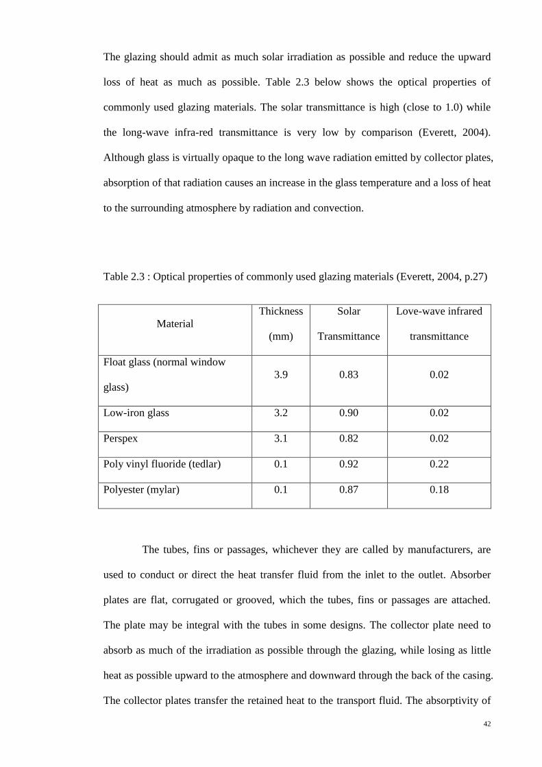
Table 2.3 : Optical properties of commonly used glazing materials (Everett, 2004, p.27)
Material
Thickness
(mm)
Solar
Transmittance
Love-wave infrared
transmittance
Float glass (normal window
glass)
3.9 0.83 0.02
Low-iron glass 3.2 0.90 0.02
Perspex 3.1 0.82 0.02
Poly vinyl fluoride (tedlar) 0.1 0.92 0.22
Polyester (mylar) 0.1 0.87 0.18
The tubes, fins or passages, whichever they are called by manufacturers, are
used to conduct or direct the heat transfer fluid from the inlet to the outlet. Absorber
plates are flat, corrugated or grooved, which the tubes, fins or passages are attached.
The plate may be integral with the tubes in some designs. The collector plate need to
absorb as much of the irradiation as possible through the glazing, while losing as little
heat as possible upward to the atmosphere and downward through the back of the casing.
The collector plates transfer the retained heat to the transport fluid. The absorptivity of
43
the collector surface for shortwave solar radiation depends on the nature and colour of
the coating and on the incident angle. The design and material selection of the plate are
the most essential items as it directly affects the efficiency of solar energy being
converted to thermal energy in the fluid. Essentially, typical selective surfaces consist of
a thin upper layer, which is highly absorbent to shortwave solar radiation but relatively
transparent to long wave thermal radiation, deposited on a surface that has a high
reflectance and a low emissivity for long wave radiation. Selective surfaces are
particularly important when the collector surface temperature is much higher than the
ambient air temperature. For fluid-heating collectors, passages must be integral with or
firmly bonded to the absorber plate. A major problem is obtaining a good thermal bond
between tubes and absorber plates without incurring excessive costs for labour or
materials. Material most frequently used for collector plates are copper, aluminium, and
stainless steel. However, even the best design will still implies certain degree of thermal
losses through conduction or convection. Reduction of heat loss from the absorber can
be accomplished either by a selective surface to reduce radiative heat transfer or by
suppressing convection. Francia (1961) and Hollands (1965) showed that a honeycomb
made of transparent material, placed in the airspace between the glazing and the
absorber, was beneficial.
The headers or manifolds are to admit and discharges the fluid while the
insulation to minimize the heat loss from the back and sides of the collector. Last but
not least, the container or casing is important as well to surround the aforementioned
components and keep them free from dust, moisture, etc.
FPC are usually employed for low temperature applications up to 100 ºC,
although some new types of collectors employing vacuum insulation and/or TI can
achieve slightly higher values (Benz, Hasler, Hetfleish, Tratzky & Klein, 1998 cited in
Kalougirou, 2004, p.243).
44
Another category of collectors is the uncovered or unglazed solar collector
(Soltau, 1992). These collectors are usually cheaper solution but still offer effective
solar thermal energy in applications such as water preheating for domestic or industrial
use, heating of swimming pools (Molineaux, Lachal & Gusian, 1994; Winter, 1994),
space heating and air heating for industrial or agricultural applications.
As one of the most common and vastly used solar thermal collector, surface
absorption type panel has its limitations. These limitations are the need of large solar
receiving area, efficiency of the surface absorber, thermal transfer loss from the black
surface absorber to the inner tube containing the fluid carrier and the surface absorber
losses to the environment due to convection and reflection. Volumetric absorber has
thus been view as a possible enhancement to the conventional surface absorption solar
collector.
2.2.3.2 Evacuated Tube Solar Collectors (ETC)
Conventional simple flat-plate solar collectors were developed for use in sunny
and warm climates. However, their performance is greatly shrunk when conditions
become unfavourable during cold, cloudy and windy days. Furthermore, weathering
influences such as condensation and moisture will cause early deterioration of internal
materials resulting in reduced performance and system failure (Kalogirou, 2004).
Evacuated heat pipe solar collectors (tubes) operate differently than the other collectors
available on the market. These solar collectors consist of a heat pipe inside a vacuum-
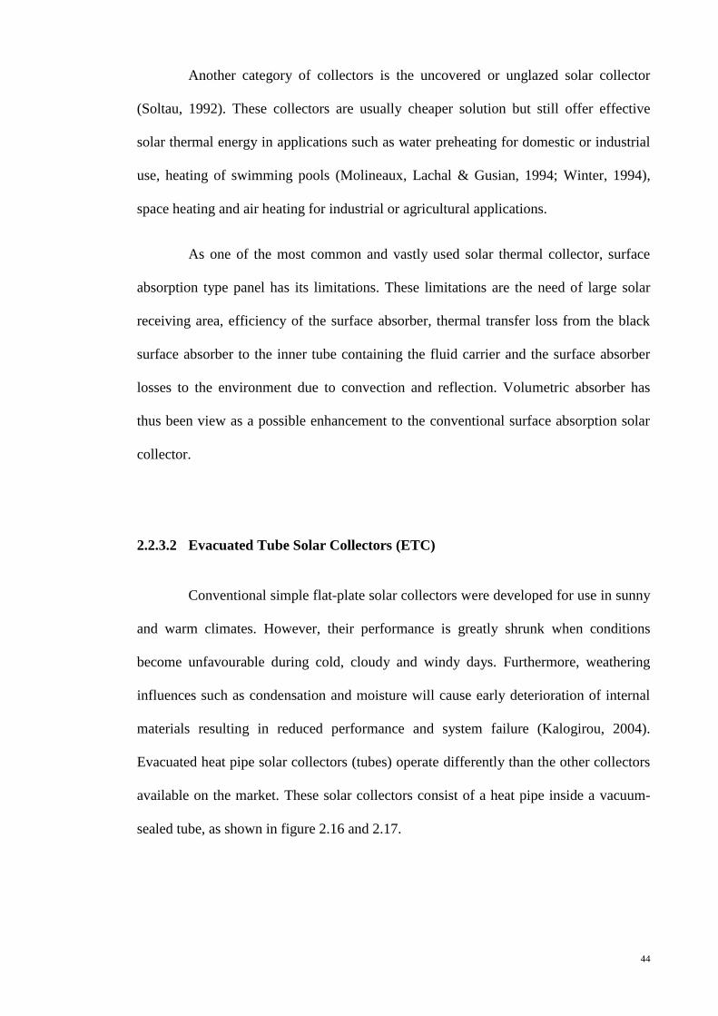
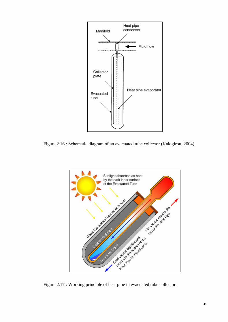
sealed tube, as shown in figure 2.16 and 2.17.
45
Figure 2.16 : Schematic diagram of an evacuated tube collector (Kalogirou, 2004).
Figure 2.17 : Working principle of heat pipe in evacuated tube collector.
46
Heat pipes are highly efficient thermal conductors with simple working
principle. It generally exploits the occurrence of natural convection in fluid when
temperature gradient arises. The pipe is a sealed copper pipe and is attached to a black
copper fin that fills the absorber plate. The top of each heat pipe is a metal tip attached
to the sealed header which serves as a condenser. The heat pipe contains a small amount
of fluid that undergoes an evaporating-condensing cycle. In this cycle, solar heat
evaporates the liquid, and the vapour travels to the heat sink region where it condenses
and releases its latent heat. The condensed fluid return back to the solar collector and
the process is repeated. Water, or glycol, flows through the manifold and picks up the
heat from the tubes. The heated liquid circulates through another heat exchanger and
gives off its heat to a process or to water that is stored in a solar storage tank.
ETC offers superior performance at high temperature compare to FPC as the
vacuum envelope reduces convection and conduction losses. ETC, similar to FPC,
collect both direct and diffuse radiation but provide higher efficiency at low incident
angles. Besides, as no evaporation or condensation above the phase-change temperature
is possible, the heat pipe offers inherent protection from freezing and overheating. This
self-limiting temperature control is a unique feature of the evacuated heat pipe collector.
These effects give ETC a higher hand compare to FPC and make it a more favourable
choice in recent years. As presented in the earlier section, the new installation of ETC
outpaced conventional FPC by far.
2.3 Nanofluid
Nanofluids, as a relatively new class of fluids, consist of a base fluid with
nano-sized particles (1–100nm) suspended within them (Saidur, et al., 2011). It is first
termed by Choi (1995) as a mixture of base fluid with a very small amount of

47
nanoparticles, dispersed uniformly and suspended stably, which can provide impressive
improvements in the thermal properties of the base fluid. A length scale of nano-size
objects is exemplified in figure 2.18.
Figure 2.18 : Length scale and some examples related (Serrano, et al., 2009)
Most things on earth comply with the saying “Size does matter”; however,
even nanoparticles are smaller than DNA, it provides a great leap forward in technology
for scientists in creating material with desired properties. These nanometers-grain-sized
materials have been found to have unique optical, electrical and chemical properties
(Gleiter, 1989). It specifically implies not only the miniaturization but also the precise
manipulation of atoms and molecules to design and control the properties of the
nanomaterials/nanosystems. These properties are completely different than those
possessed by the bulk materials, which helps in constructing custom-made devices with
capabilities not found in bulk materials or in nature, or even to replicate some natural
processes that have not been currently achieved through synthetic materials (Serrano, et
al., 2009).
The idea of volumetric absorption using small particles has been proposed long
before the ability to controllably synthesize nanoparticles was developed. In the 1970s,
48
large temperature differences at the interface between the absorber and the heat transfer
fluid were identified, and particle-based volumetric absorbers for solar central-receivers
were proposed by Hunt (1978) and Abdelrahman (1979). Attempts of using black
liquids, for instance water soluble dyes, as the absorbing medium were brought up by
Minardi and Chunag (1975). Tyagi et al. (2009) investigated the feasibility of using a
non-concentrating direct absorption solar collector (DAC) and compares its
performance with that of a typical flat-plate collector. He used a mixture of water and
aluminium nanoparticles as the nanofluid and found that with the presence of
nanoparticles, the absorption of incident radiation is increased by nine times over that of
pure water. The efficiency of DAC using nanofluid as the working fluid is found to be
up to 10% higher (on an absolute basis) than that of a flat-plate collector. This shows a
promising improvement to conventional heat collector and further study and research
are encouraged.
The technology of nanofluid has been implemented in parabolic trough solar
collectors for years. However, without the mirrors used to reflect and concentrate solar
radiant in the parabolic trough solar collectors, the fluid used for volumetric direct solar
collectors is ought to possess excellent optical properties beside conventional
requirement of good thermal transfer properties. Researches on thermal behavior of
nanofluids have been done extensively over the pass decades and many correlations had
been set-up and confirmed with experiments. However, the research on optical
properties of nanofluid has shown slower progress. The numerous parameters such as
physical and optical properties of base fluid and nanoparticles and the concentration of
nanoparticles used have been some major investigation topics or obstacles for
researchers to understand the solar absorption behavior of nanofluid.
49
2.3.1 Optical Properties of Nanofluid
In order to properly design a nanofluid-based solar collector it is important to
develop a basic understanding of the radiative properties of nanofluids. Nanofluid
consists of two main components which are the nanoparticles and the base fluid.
Nanoparticles are added into water or refrigerant to improve and alter the optical
properties of the fluid to become more solar favourable. In the base fluid point of view,
a study of solar-weighted absorption coefficient for fluid‟s baseline capacity for
absorbing solar energy by Otanicar, et al. (2009) suggested that water is the best
absorber among the four tested liquids namely water, ethylene glycol, propylene glycol
and therminol VP-1. However, it is still a weak absorber, only absorbing 13% of the
energy.
On the other hand, the addition of small particles causes scattering of the
incident radiation allowing higher levels of absorption within the fluid, and hence an
enhancement in collector efficiency (Tyagi, 2008). The optical properties of the
effective fluid are highly dependent on the shape and size of the particle, and the optical
properties of the base fluid and particles themselves (Khlebtsov et al., 2005). The
radiation absorption characteristics of a Ni nanoparticle suspension were investigated by
spectroscopic transmission measurement by Kameya and Hanamura (2011). It was
demonstrated that the absorption coefficient of the nanoparticle suspension is much
higher than that of the base liquid for visible to near-infrared wavelengths. Radiation
characteristics predicted by the Mie theory showed good agreement with the increase of
absorption coefficient in wavelengths where the base liquid is transparent. Recently,
carbon nanohorns (CNHs), as the latest to be discovered in the family of carbon-based
nanostructured materials (Iijima, 1999), with large surface area and large number of
cavities (Fan, 2007), were used as nanoparticles to improve optical properties of direct
solar absorbers. The studies showed promising improvement of absorption and

50
scattering properties for carbon nanohorns-based nanofluid with compare to water and
glycol as base fluid (Sani, et al., 2010; Mercatelli, et al., 2011).
The temperature difference between the absorbing particles and the fluid has
been shown to be negligible owing to the particles‟ large surface to volume ratio
(Minardi and Chunag, 1975; Miller, F. J., and Koenigsdorff, R. W., 2000). The
temperature dependence of the optical/spectroscopic properties of metallic nanoparticles
(in particular nanoshells) including absorption, scattering, and enhanced-Raman
scattering for admolecules is studied via theoretical modelling by Chen et al. (2008). It
is suggested that these properties in general have optimal values at a certain temperature
specific to the shell configuration except for relatively thin shells.
The optical absorption of nanofluid also depends on the concentration or
volume/weight fraction of nanoparticles added to the base fluid. Both researches
published by Mishra et al. on year 2008 and 2009 showed a shift of absorption spectra
towards longer wavelength in nanofluid with higher concentration. Carbon nanotubes,
graphite, and silver were used as nanoparticles and by utilizing nanofluids as the
absorption mechanism in solar thermal collectors; it was demonstrated efficiency
improvements of up to 5% (Otanicar, et al., 2010). In addition, their experimental data
were compared with a numerical model of a solar collector with direct absorption
nanofluids. The experimental and numerical results demonstrated an initial rapid
increase in efficiency with volume fraction, followed by a leveling off in efficiency as
volume fraction continues to increase.
Further to optical properties, the addition of nanoparticles to a base fluid has
been shown to improve thermal conductivity. Studies suggested that the thermal
conductivity is enhanced due to dispersion of nanoparticles (Pak and Cho, 1998; Xuan
and Li, 2000), intensification of turbulence (Xuan and Li, 2000), Brownian motion

51
(Keblinski et al., 2002; Koo and Kleinstreuer, 2005), thermophoresis and
diffusiophoresis (Buongiorno, 2006). The application of nanofluids as a working
medium for solar collectors is a relatively new concept. Further study on the physical
properties in help of enhancing direct solar collectors has to be carried out.
In this thesis, the optical properties of nanofluid are studied and the
transmissivity of base fluid and nanofluid is compared. From section 2.1, we can
determine that the nanoparticles proposed for this study should be of size lesser than 10%
of the incident wavelength as Rayleigh scattering will not be valid anymore if the size
of nanoparticles exceeded this size. This limits the size of nanoparticles to be around 20
nm. Adding to the above, since ETC provides good solar to thermal energy conversion
efficiency, the use of nanofluid in replacing the working fluid in the heat pipes may be
considered. However, as the fundamental working principle of a heat pipe is by natural
convection and no mechanical force is added, the volume fraction of nanoparticles in
the nanofluid should not be too much. This is to avoid clogging of working fluid in heat
pipes and eventually reduce their effectiveness.
52
Chapter 3: Methodology
3.0 Introduction
This chapter is divided into two components. The first component or section
describes the working principle and some equations to calculate the incident solar
intensity and transmissivity of Direct Absorption Collector (DAC).The second section
in this chapter will explain and demonstrate the governing equations used for nanofluid
to develop its optical properties.
3.1 Direct Absorption Collector (DAC)
Solar water heating technologies are becoming widespread and contribute
significantly to hot water production in several countries. China, Germany, Turkey,
India, and Australia led the market for newly installed capacity during 2009, with China,
Turkey, Germany, Japan, and Greece taking the top spots for total installations by the
end of that year (REN 21, 2011). Although with such popularity, these types of solar
collectors exhibit several shortcomings, such as limitations on incident flux density,
relatively high losses, and corrosion effect. In order to overcome these drawbacks, the
idea of using volumetric direct solar collectors is raised.
Direct Absorption Solar Collector (DAC) has a few advantages compare to
conventional surface absorption collector. Besides larger solar absorption area and
actual installation surface area ratio due to the contribution of nanoparticle surface area,
DAC can avoid surface heat losses due to excessive temperature on surface absorption
collector. For a black body receiver, the radiative losses scale as the fourth power of the
temperature, as seen in figure 3.1. For surface solar absorber, the efficiency sharply
drops with increasing temperature. To suppress radiative heat loss from the receiver,

53
selective surfaces are manufactured to have low emissivity at the longer wavelengths
which correspond to thermal radiation. However, the performance of a receiver at high
temperatures is limited by the Kirchoff‟s Law, which states that the spectral absorptivity
must equal the spectral emissivity. In other words, since an absorber is absorptive for
wavelength in the solar spectrum, it consequently emits in those same wavelengths
which leads to a lower absorber efficiency. Figure 3.1 illustrates how the power losses
from an ideal selective surface exhibit the same forth order dependence on the absorber
temperature as a black body except the trend is shifted to higher temperature (Lenert,
2010).
Figure 3.1 : Power loss due to re-radiation as a function of temperature: from a black
body (black), and a selective surface (green) (Lenert, 2010).

54
The convection losses to the ambient air also become significant as the
temperature difference between the absorber surface and ambient air become larger.
This is a simple demonstration of heat transfer by convection with equation of :
By using nanofluid as volumetric absorber, the drawbacks of surface emission
and convection heat loss can be eliminated. A schematic of the difference of surface
absorber versus volumetric receiver utilizing nanofluid to absorb solar radiation is
illustrated in Figure 3.2.
Figure 3.2 : Difference between surface-based and volumetric solar absorbers (Lenert,
2010).
The schematic of the nanofluid-based Direct Absorption Solar Collector (DAC)
is shown in Figure 3.3. The fluid is contained within the enclosed space of the DAC.
The bottom wall is considered to be adiabatic, i.e. no heat flux is allowed to pass
through it, except for transmitted radiation. This assumption is based on the case when
the bottom surface is highly insulating and transparent. The fluid is enclosed at the top

55
by a glass surface which allows most of the incident solar flux to pass through. This top
surface is assumed to be exposed to the ambient atmosphere and thus loses heat by
convection. In order to model the heat transfer characteristics of this surface it is
assumed that it loses heat to the ambient through convection. The incident radiation is
considered to be the incoming solar radiation. For the study of the principal behavior of
the nanofluid-based DAC, atmospheric absorption was neglected in these calculations.
Hence, the incident solar intensity is calculated using the blackbody relation given by
Eq. (3.1), where the value of Tsolar is taken as 5800 K (Tyagi, 2008; Tyagi, Phelan &
Prasher, 2009).
Figure 3.3 : Schematic of the nanofluid-based direct absorption solar collector (DAC)
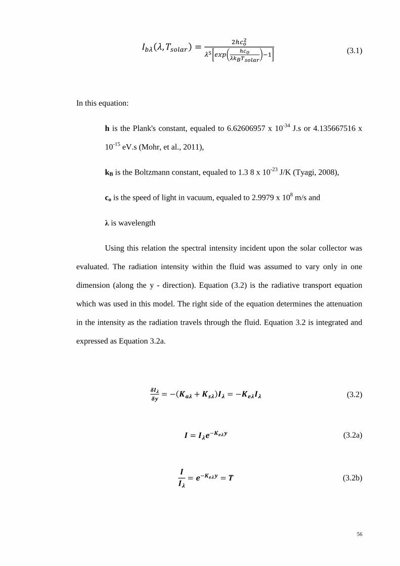
56
( )
[ (
) ]
(3.1)
In this equation:
h is the Plank's constant, equaled to 6.62606957 x 10⁻³⁴
J.s or 4.135667516 x
10-15
eV.s (Mohr, et al., 2011),
kB is the Boltzmann constant, equaled to 1.3 8 x 10-23
J/K (Tyagi, 2008),
co is the speed of light in vacuum, equaled to 2.9979 x 10⁸ m/s and
λ is wavelength
Using this relation the spectral intensity incident upon the solar collector was
evaluated. The radiation intensity within the fluid was assumed to vary only in one
dimension (along the y - direction). Equation (3.2) is the radiative transport equation
which was used in this model. The right side of the equation determines the attenuation
in the intensity as the radiation travels through the fluid. Equation 3.2 is integrated and
expressed as Equation 3.2a.
( ) (3.2)
(3.2a)
(3.2b)
57
where Kaλ is the spectral absorption coefficient, and Ksλ the spectral scattering
coefficient. Taken together they can also be represented as Keλ, the spectral extinction
coefficient where I, denotes the transmitted light intensity. Equation 3.2a confirmed that
the intensity of light transmitted is inverse to the length of light path, y and is further
rearrange to become equation 3.2b to obtain Transmissivity, T. This agrees with the
Beer-Lambert Law. Since the temperatures in the solar collector are not expected to be
very high, the emission term has not been included in Eq. (3.2). Also, in order to keep
the model simple the effect of in-scattering has not been considered.
3.2 Radiative Properties of Nanofluid
The study of optical properties of nanofluid shows the need to study optical
properties of the based fluid and nanoparticles separately. The brief theory and relation
of light scattering and extinction for base fluid and nanoparticles are presented below.
3.2.1 Radiative Properties of Base Fluid
In order to fully understand the effects of suspending nanoparticles within a
base fluid, the complete optical properties of the base fluid are needed. The bulk of the
volumetric receiver is the fluid medium; therefore, the radiative properties of the fluid
are critical to the efficiency of a volumetric design. An ideal fluid for a volumetric
application would be completely transparent to the incoming solar radiation (Lenert,
2010). Base fluid normally used in direct solar collectors like water heater has to be
non-toxic.
A study of solar-weighted absorption coefficient for fluid‟s baseline capacity
for absorbing solar energy by Otanicar, et al. (2009) suggested that water is the best

58
absorber among the four tested liquids namely water, ethylene glycol, propylene glycol
and therminol VP-1. However, it is still a weak absorber, only absorbing 13% of the
energy. Another later study by Mercatelli et al. (2011) on absorption and scattering
properties of carbon nanohorn-based nanofluids for DAC using glycol and water as base
fluid also showed a more advantageous improvement from water-based nanofluid.
Figure 3.4 below is extracted from Mercatelli et al.‟s study to show the transmittance
spectra of water and glycol-based nanofluids with the same Single Wall Carbon
Nanohorn (SWCNH) concentrations. However, preliminary thermal stability tests
performed showed that water-based suspensions are stable up to 120°C, while glycol-
based suspensions are stable up to 150°C. An improvement of the thermal stability
properties of the nanofluid should be expected by an optimization of SWCNH-
surfactant concentration ratio. Despite the more superior performance of glycol-based
nanofluid at high temperature, water is chosen to be the base fluid to study here as DAC
is targeted to be used mainly in residential development and working temperature is
estimated to be low.

59
Figure 3.4 : Transmittance spectra of water and glycol-based nanofluids with the same
SWCNH concentrations (0.005 g/L for G1 and A1 and 0.05 g/L for G4 and A4).
Spectra of the pure base fluids are shown for comparison (G0 and A0) (Mercatelli,
2011).
For pure fluids, scattering can be neglected and only the attenuation caused by
absorption may be considered. For that case, the spectral absorption coefficient can be
calculated using Eq. (3.3),
(3.3)
where k is the index of absorption and λ is the wavelength of incident light.
The definitive data on the absorption spectrum of pure water from 200 nm to
3500 nm had been obtained by Irvine and Pollack (1968, cited in Brewster, 1992).
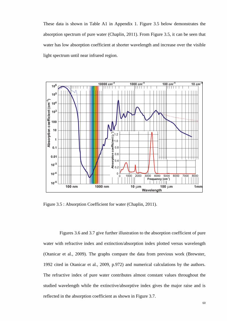
60
These data is shown in Table A1 in Appendix 1. Figure 3.5 below demonstrates the
absorption spectrum of pure water (Chaplin, 2011). From Figure 3.5, it can be seen that
water has low absorption coefficient at shorter wavelength and increase over the visible
light spectrum until near infrared region.
Figure 3.5 : Absorption Coefficient for water (Chaplin, 2011).
Figures 3.6 and 3.7 give further illustration to the absorption coefficient of pure
water with refractive index and extinction/absorption index plotted versus wavelength
(Otanicar et al., 2009). The graphs compare the data from previous work (Brewster,
1992 cited in Otanicar et al., 2009, p.972) and numerical calculations by the authors.
The refractive index of pure water contributes almost constant values throughout the
studied wavelength while the extinctive/absorptive index gives the major raise and is
reflected in the absorption coefficient as shown in Figure 3.7.

61
Figure 3.6 : Calculated and published values of Refractive Index, n of water (Otanicar et
al., 2009)
Figure 3.7 : Calculated and published values of Extinction Index, k of water (Otanicar et
al., 2009)
62
Since the optical properties had long been study and data is verified by many
researchers (Brewster, 1992; Kou, Labrie and Chylek, 1996; IAPWS, 1997; Pope and
Fry, 1997; Otanicar et al., 2009; Chaplin, 2011), the spectrum of absorption coefficient
used for calculation in this study will be based on the published data from previous
work. The data used is by Brewster (1992) and Table A1 is referred.
3.2.2 Radiative Properties of Nanoparticles
When it comes to studying of optical properties of nanoparticles, there are a
few assumptions to be made in order to simplify the complexity of equations involved.
Firstly, it is assumed that the nanoparticles are experiencing independent
scattering. The inhomogeneous of nanoparticles in base fluid can see to be “alien”
bodies immerse in a medium. It can be seen as dust or haze in the atmosphere or sand or
mud in clear river water. However, if such particles are sufficiently far from each other,
it is possible to study the scattering by one particle without reference to the other ones.
This is called “independent scattering” (van de Hulst, 1981). But one may ask, what
distance between the particles is sufficiently large to ensure independent scattering?
Early estimates have shown that a mutual distance of 3 times the radius is a sufficient
condition for independence (van de Hulst, 1981). In this study, the nanoparticles are
provided in a very small size and the volume fraction is only a small portion of the base
fluid. Thus, the scattering effect of nanoparticles in nanofluid can be considered to be
independent.
Further to this, the scattering effect studied here is assumed to be of single
scattering. Practical experiments most often employ a multitude of similar particles in a
cloud or a solution, namely nanofluid. The obvious relations for a nanofluid containing

63
X scattering particles are that the intensity scattered by the fluid is X times that scattered
by a single particle, and the energy removed from the original beam is also X times that
removed by a single particle. This simple proportionality to the number of particles
holds only if the radiation to which each particle is exposed is essentially the light of the
original beam. In actuality, each particle is also exposed to light scattered by the other
particles, whereas the light of the original beam may have suffered extinction by the
other particles. If these effects are strong, we speak of multiple scattering and a simple
proportionality does not exist. This situation may be illustrated by a white cloud in the
sky. Such a cloud is like a dense fog; its droplets may be considered as independent
scatter. Yet the total intensity scattered by the cloud is not proportional to the number of
droplets contained in it, for not each droplet is illuminated by full sunlight. Drops within
the cloud may receive no direct sunlight at all but only diffuse light which has been
scattered by two or more droplets successively (van de Hulst, 1981). This multiple
scattering effect is neglected in this study to abridge the calculations and relationships
of light extinction.
In this study of nanofluids, where the presence of small particles influences the
nature of absorption as well as scattering, Rayleigh scattering (Bohren & Huffman,
1983) can be applied. The particles are assumed to be spherical and the medium to be
non-absorbing. This is merely for simplification of studying Rayleigh scattering effect
while the effect of absorption of the base fluid, water, will be added into the main
calculation later on.
In Rayleigh scattering α < 1 and |m| α < 1, where α is defined as the size
parameter and m is the normalized refractive index of the particles to the fluid. They are
given by (Prasher, 2007; Tyagi, 2008; Tyagi, Phelan and Prasher, 2009; Otanicar et al.,
2010):
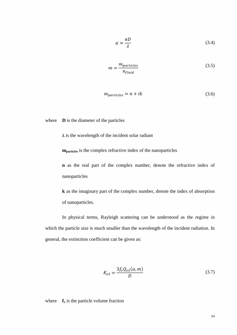
64
(3.4)
(3.5)
(3.6)
where D is the diameter of the particles
λ is the wavelength of the incident solar radiant
mparticles is the complex refractive index of the nanoparticles
n as the real part of the complex number, denote the refractive index of
nanoparticles
k as the imaginary part of the complex number, denote the index of absorption
of nanoparticles.
In physical terms, Rayleigh scattering can be understood as the regime in
which the particle size is much smaller than the wavelength of the incident radiation. In
general, the extinction coefficient can be given as:
( )
(3.7)
where fv is the particle volume fraction
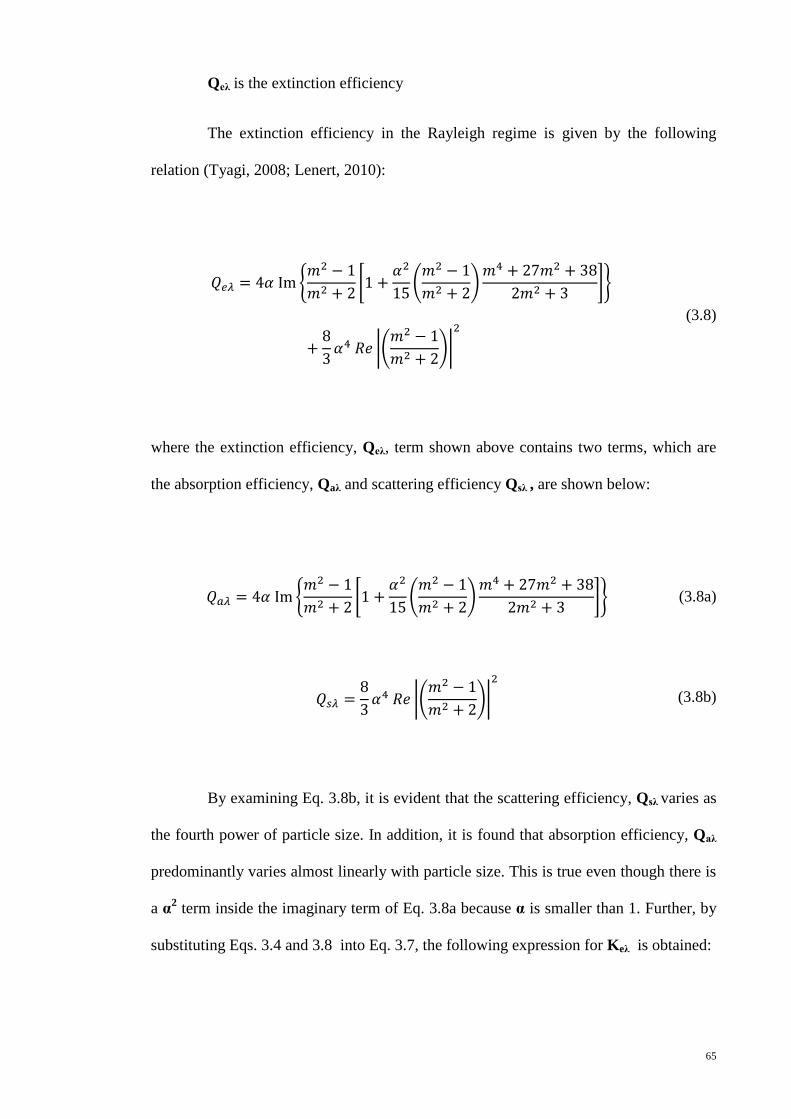
65
Qeλ is the extinction efficiency
The extinction efficiency in the Rayleigh regime is given by the following
relation (Tyagi, 2008; Lenert, 2010):
,
*
(
)
+-
|(
)|
(3.8)
where the extinction efficiency, Qeλ, term shown above contains two terms, which are
the absorption efficiency, Qaλ and scattering efficiency Qsλ , are shown below:
,
*
(
)
+- (3.8a)
|(
)|
(3.8b)
By examining Eq. 3.8b, it is evident that the scattering efficiency, Qsλ varies as
the fourth power of particle size. In addition, it is found that absorption efficiency, Qaλ
predominantly varies almost linearly with particle size. This is true even though there is
a α2 term inside the imaginary term of Eq. 3.8a because α is smaller than 1. Further, by
substituting Eqs. 3.4 and 3.8 into Eq. 3.7, the following expression for Keλ is obtained:

66
,
*
(
)
+-
|(
)|
(3.9)
where the extinction coefficient, Keλ term shown above contains two terms, which are
the absorption coefficient Kaλ and scattering coefficient, Ksλ. They are shown below.
,
*
(
)
+- (3.9a)
|(
)|
(3.9b)
Lenert (2010) suggested that the two complex expressions in Eq. 3.8 can be
greatly simplified if the terms with a higher order of the size parameter, α, are neglected
because this parameter is small in the case of nanoparticles. It was assumed that the
amount of incident radiation absorbed by the nanoparticle is dominated over the amount
of scattering by the particle. Since scattering is neglected, the attenuated light is
assumed to be absorbed; thus the extinction coefficient is merely just absorption
coefficient (Lenert, 2010). Equation 3.9 is greatly simplified to become as below:
,
- (3.10)
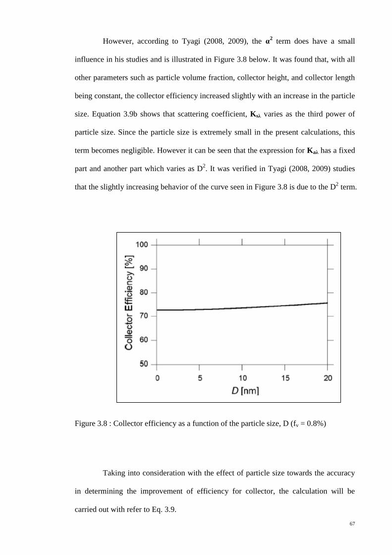
67
However, according to Tyagi (2008, 2009), the α2 term does have a small
influence in his studies and is illustrated in Figure 3.8 below. It was found that, with all
other parameters such as particle volume fraction, collector height, and collector length
being constant, the collector efficiency increased slightly with an increase in the particle
size. Equation 3.9b shows that scattering coefficient, Ksλ varies as the third power of
particle size. Since the particle size is extremely small in the present calculations, this
term becomes negligible. However it can be seen that the expression for Kaλ has a fixed
part and another part which varies as D2. It was verified in Tyagi (2008, 2009) studies
that the slightly increasing behavior of the curve seen in Figure 3.8 is due to the D2 term.
Figure 3.8 : Collector efficiency as a function of the particle size, D (fv = 0.8%)
Taking into consideration with the effect of particle size towards the accuracy
in determining the improvement of efficiency for collector, the calculation will be
carried out with refer to Eq. 3.9.

68
Finally, by using Eqs. 3.5 and 3.8, the radiative properties of the nanofluid
were evaluated. The net extinction caused by the nanofluid was obtained by adding the
individual contributions from the nanoparticles as well as the base fluid. The intensity
distribution within the solar collector was obtained using:
( ) (3.11)
where, Kaλ,water and Keλ,nanoparticles are obtained from Eqs. 3.3 and 3.9 respectively.
When the volume fraction of nanoparticles is low the contributions of
nanoparticles and base fluid could be added together as shown in Equation 3.11. This is
because the present model assumes independent scattering, where the scattered
radiations do not depend on one another and hence the intensities can be added. The
equations above mentioned are used to learn the effect of nanofluid in direct solar
collector.
69
Chapter 4: Results and Discussions
4.0 Introduction
With the aid of the equations set up and developed by researchers, the
extinction coefficient of nanofluid with water as base fluid and aluminium as
nanoparticles are studied.
Aluminium is chosen to be the nanoparticles for this study as it is one of the
common and vastly available metals. Besides, the thermal properties of aluminium
enhanced nanofluid have been studied extensively over the pass decades and had shown
promising improvement to the thermal properties. The optical properties of aluminium
are obtained from work by preceding researchers (Smith, Shiles and Inokuti, 1985) and
are displayed with normalized value of Refractive index, n’, and Absorption index, k’
calculated using equation 3.5 in Table A2 in Appendix 1.
The effects of nanoparticles in enhancing the optical properties of base fluid
are explored with nanoparticle sizes and volume fraction as parameters. As mentioned
in the previous chapter, nanoparticles proposed for this study should be of size lesser
than 10% of the incident wavelength as Rayleigh scattering will not be valid anymore if
the size of nanoparticles exceeded this size. This will limit the size of nanoparticles to
20 nm as incident solar intensity has most concentration starts from about 200 nm. The
volume fraction of nanoparticles in the nanofluid is also to be a smaller percentage to
allow possibility of applying the results to ETC and to avoid shifting of the maximum
absorption coefficient of nanofluid to the longer wavelength which has lesser
concentration. The maximum volume fraction, fv, is set to be 8% in this review.
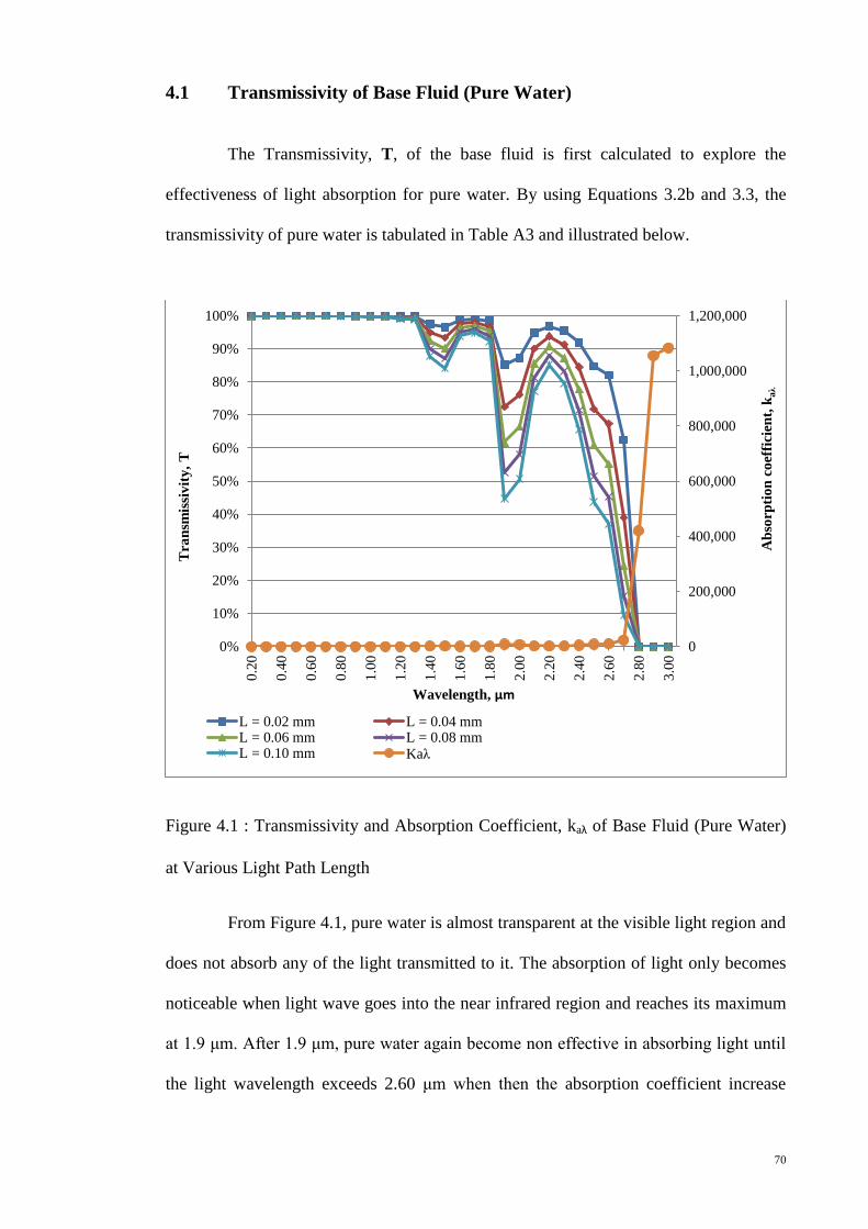
70
4.1 Transmissivity of Base Fluid (Pure Water)
The Transmissivity, T, of the base fluid is first calculated to explore the
effectiveness of light absorption for pure water. By using Equations 3.2b and 3.3, the
transmissivity of pure water is tabulated in Table A3 and illustrated below.
Figure 4.1 : Transmissivity and Absorption Coefficient, kaλ of Base Fluid (Pure Water)
at Various Light Path Length
From Figure 4.1, pure water is almost transparent at the visible light region and
does not absorb any of the light transmitted to it. The absorption of light only becomes
noticeable when light wave goes into the near infrared region and reaches its maximum
at 1.9 μm. After 1.9 μm, pure water again become non effective in absorbing light until
the light wavelength exceeds 2.60 μm when then the absorption coefficient increase
0
200,000
400,000
600,000
800,000
1,000,000
1,200,000
0%
10%
20%
30%
40%
50%
60%
70%
80%
90%
100%
0.2
0
0.4
0
0.6
0
0.8
0
1.0
0
1.2
0
1.4
0
1.6
0
1.8
0
2.0
0
2.2
0
2.4
0
2.6
0
2.8
0
3.0
0
Ab
sorp
tio
n c
oef
fici
ent,
kaλ
Tra
nsm
issi
vit
y,
T
Wavelength, μm
L = 0.02 mm L = 0.04 mmL = 0.06 mm L = 0.08 mmL = 0.10 mm Kaλ

71
sharply and transmissivity dropped abruptly. In general, pure water is not an effective
light absorber especially in the visible light region.
4.2 Optical Properties of Nanoparticles
The study on the effect in enhancing optical properties of nanofluid by
aluminium nanoparticles starts with choosing the suitable nanoparticle size. As
mentioned earlier, the particle size is limited to below 20 nm. The absorption coefficient,
kaλ, scattering coefficient, ksλ and extinction coefficients, keλ of aluminium nanoparticle
of few sizes namely 1 nm, 5 nm, 10 nm, 15 nm and 20 nm are calculated with Equations
3.9a, 3.9b and 3.9 with the volume fraction set to be 2%. The results are tabulated in
Table A4, A5 and A6 and graphs are established to show the trend and pattern of
increasing nanoparticle sizes.
Figure 4.2 : The Effect of Nanoparticle Sizes towards Absorption Coefficient, kaλ
0
200,000
400,000
600,000
800,000
1,000,000
1,200,000
1,400,000
1,600,000
1,800,000
0.2
0
0.4
0
0.6
0
0.8
0
1.0
0
1.2
0
1.4
0
1.6
0
1.8
0
2.0
0
2.2
0
2.4
0
Ab
sorp
tion
Coef
fici
ent,
ka
λ
Wavelength, μm
D = 1.0 nm D = 5.0 nm D = 10.0 nm D = 15.0 nm D = 20.0 nm
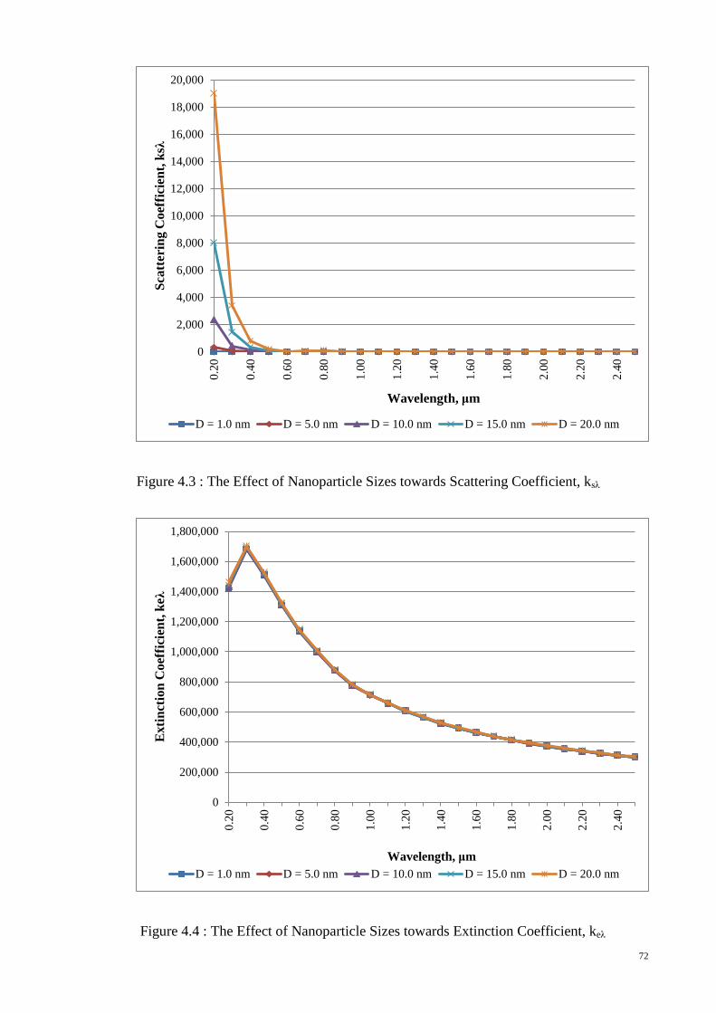
72
Figure 4.3 : The Effect of Nanoparticle Sizes towards Scattering Coefficient, ksλ
Figure 4.4 : The Effect of Nanoparticle Sizes towards Extinction Coefficient, keλ
0
2,000
4,000
6,000
8,000
10,000
12,000
14,000
16,000
18,000
20,000
0.2
0
0.4
0
0.6
0
0.8
0
1.0
0
1.2
0
1.4
0
1.6
0
1.8
0
2.0
0
2.2
0
2.4
0
Sca
tter
ing
Co
effi
cien
t, k
sλ
Wavelength, μm
D = 1.0 nm D = 5.0 nm D = 10.0 nm D = 15.0 nm D = 20.0 nm
0
200,000
400,000
600,000
800,000
1,000,000
1,200,000
1,400,000
1,600,000
1,800,000
0.2
0
0.4
0
0.6
0
0.8
0
1.0
0
1.2
0
1.4
0
1.6
0
1.8
0
2.0
0
2.2
0
2.4
0
Exti
nct
ion
Coef
fici
ent,
keλ
Wavelength, μm
D = 1.0 nm D = 5.0 nm D = 10.0 nm D = 15.0 nm D = 20.0 nm
73
Figure 4.2, 4.3 and 4.4 demonstrates the absorption coefficient, scattering
coefficient and extinction coefficient of aluminium nanoparticles versus light
wavelength with particle size as the parameter.
From Figure 4.2, it should be noted that there are five lines in the graph
although the lines overlapped each other and only two very close lines (blue line and
brown line which denote particle size of 1 nm and 20 nm respectively) are shown. The
differences of absorption coefficient between particle sizes are tabulated in Table A4 in
Appendix 1 and only very small differences are spotted at wavelength shorter than 0.6
μm. The differences are within 1.5% between the smallest and largest particle size
calculated. The data shows identical absorption coefficient for the different sizes after
0.6 μm. This can be explained from equation 3.9a. The particle size in nanometer
becomes very insignificant to the overall equation after being squared and also divided
by the wavelength term in micrometer. The further increase in wavelength will
overshadow the effect of particle size and eventually leads to near-constant absorption
coefficient.
Figure 4.3 illustrated a similar trend as the absorption coefficient graph. The
effect of different particle size become almost unnoticeable after wavelength is longer
than 0.6 μm. This can be explained also by looking at the governing equation. The
particle size is in power of three while wavelength is in power of four. In near UV
region, where wavelength is shorter, the effect of having larger particles is still obvious.
As wavelength becomes longer and the scattering coefficient is inversely proportional to
the wavelength with power of four, the effect is minimized. Detail data is presented in
Table A5 in Appendix 1.
Figure 4.4 is almost similar to figure 4.2. As described in Equation 2.4 and
3.9, the extinction coefficient is the sum of scattering coefficient and absorption
74
coefficient. The much smaller Scattering coefficient demonstrates no noteworthy
influence to the overall extinction coefficient calculation. In short, particles used in
nanofluid are extremely small and the terms D2 and D
3 have very little impact to the
Extinction coefficient equation. This is in common to the study by Lenert (2010) who
suggested that the size of nanoparticle is not a deciding factor to the optical properties
of nanofluid and the extinction coefficient is simply dependent on the optical properties
in suspension and the total volume fraction. However, it is theoretically expected that
the higher particle size should lead to higher extinction coefficient. However, as
mentioned in the previous chapter, in order to apply Rayleigh scattering, the particle
size has to be controlled within 20 nm. Since the particle size shows not much influence
to the optical properties, particle size of 10 nm is simply picked for the following study
in the effect of volume fraction to the optical properties.
Figure 4.5 and 4.6 illustrated the absorption coefficient spectrum for
aluminium nanoparticles with particle size of 10 nm. The calculated data that served as
the basis of these graphs are presented in Appendix 1 as Table A7 and A7a. Both the
graph and data are divided into two sets, which the first set is with volume fraction
increasing by 0.5% and the second set increasing by 1.0% at every interval, in order to
study the sensitivity of volume fraction of nanoparticles towards its absorption
coefficient.

75
Figure 4.5 : The Effect of Nanoparticle Volume Fraction, fv (0.1% - 2.5%) towards
Absorption Coefficient, kaλ
Figure 4.6 : The Effect of Nanoparticle Volume Fraction, fv (1.0% - 8.0%) towards
Absorption Coefficient, kaλ
0
500,000
1,000,000
1,500,000
2,000,000
2,500,000
0.2
0
0.4
0
0.6
0
0.8
0
1.0
0
1.2
0
1.4
0
1.6
0
1.8
0
2.0
0
2.2
0
2.4
0
Ab
sorp
tio
n C
oef
fici
ent,
ka
λ
Wavelength, μm
fv = 0.1 % fv = 0.5 % fv = 1.0 % fv = 1.5 % fv = 2.0 % fv = 2.5 %
0
1,000,000
2,000,000
3,000,000
4,000,000
5,000,000
6,000,000
7,000,000
8,000,000
0.2
0
0.4
0
0.6
0
0.8
0
1.0
0
1.2
0
1.4
0
1.6
0
1.8
0
2.0
0
2.2
0
2.4
0
Ab
sorp
tion
Coef
fici
ent,
ka
λ
Wavelength, μm
fv = 1.0 % fv = 2.0 % fv = 3.0 % fv = 4.0 %
fv = 5.0 % fv = 6.0 % fv = 7.0 % fv = 8.0 %

76
From Figures 4.5 and 4.6, we can see that the absorption coefficient gains it
weight sharply from wavelength of 0.2 μm to slightly before 0.3 μm and ease with
almost the same pace along the visible light region. The absorption coefficient slowly
comes to a constant decreasing gradient after wavelength of 0.9 μm and continues all
the way through the studied wavelengths. This phenomenon happens to every volume
fraction calculated but however, larger volume fraction shows sharper rise and drop
fashion. In general, absorption coefficient upsurges with the increase of volume fraction
with the same rate. Absorption coefficient is linearly proportional to volume fraction
and this can be confirmed from equation 3.9a.
Besides absorption coefficient, the scattering coefficient of aluminium
nanoparticles is shown. Figures 4.7 and 4.8 display the trend of scattering coefficient
along various light wavelengths while Table A8 and A8a give the developed data.
Figure 4.7 : The Effect of Nanoparticle Volume Fractions, fv (0.1% - 2.5%) towards
Scattering Coefficient, ksλ
0
500
1,000
1,500
2,000
2,500
3,000
3,500
0.2
0
0.4
0
0.6
0
0.8
0
1.0
0
1.2
0
1.4
0
1.6
0
1.8
0
2.0
0
2.2
0
2.4
0
Sca
tter
ing C
oef
fici
ent,
ksλ
Wavelength, μm
fv = 0.1 % fv = 0.5 % fv = 1.0 % fv = 1.5 % fv = 2.0 % fv = 2.5 %

77
Figure 4.8 : The Effect of Nanoparticle Volume Fractions, fv (2.0% - 8.0%) towards
Scattering Coefficient, ksλ
Similar to the graphs plotted for absorption coefficient, the trends are shown in
two set of graphs to learn the sensitivity of scattering coefficient towards volume
fraction. Figure 4.7 demonstrates the spectrum of scattering coefficient with interval of
0.5% increment of volume fraction while figure 4.8 gives 2.0% of increment. According
to Figures 4.7 and 4.8, aluminium nanoparticles only contribute to scattering coefficient
at a very small region. The scattering coefficients are large and significant at near UV
section around 0.2 μm and it follows by an abrupt descent to close to nil when entering
the visible light section. The scattering coefficient of nanoparticle decreases to below
100 at wavelength of 0.3 μm and reach zero after wavelength of 0.5 μm. The increment
of volume fraction gives larger scattering coefficient but yet it turns out to be negligible
after 0.3 μm of wavelength. This further proved that scattering coefficient can be
0
1,000
2,000
3,000
4,000
5,000
6,000
7,000
8,000
9,000
10,000
0.2
0
0.4
0
0.6
0
0.8
0
1.0
0
1.2
0
1.4
0
1.6
0
1.8
0
2.0
0
2.2
0
2.4
0
Sca
tter
ing
Co
effi
cien
t, k
sλ
Wavelength, μm
fv = 2.0 % fv = 4.0 % fv = 6.0 % fv = 8.0 %
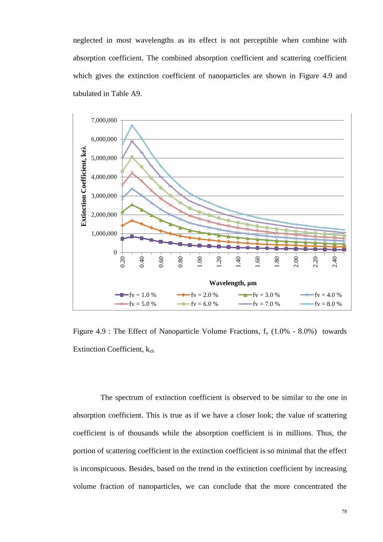
78
neglected in most wavelengths as its effect is not perceptible when combine with
absorption coefficient. The combined absorption coefficient and scattering coefficient
which gives the extinction coefficient of nanoparticles are shown in Figure 4.9 and
tabulated in Table A9.
Figure 4.9 : The Effect of Nanoparticle Volume Fractions, fv (1.0% - 8.0%) towards
Extinction Coefficient, keλ
The spectrum of extinction coefficient is observed to be similar to the one in
absorption coefficient. This is true as if we have a closer look; the value of scattering
coefficient is of thousands while the absorption coefficient is in millions. Thus, the
portion of scattering coefficient in the extinction coefficient is so minimal that the effect
is inconspicuous. Besides, based on the trend in the extinction coefficient by increasing
volume fraction of nanoparticles, we can conclude that the more concentrated the
0
1,000,000
2,000,000
3,000,000
4,000,000
5,000,000
6,000,000
7,000,0000
.20
0.4
0
0.6
0
0.8
0
1.0
0
1.2
0
1.4
0
1.6
0
1.8
0
2.0
0
2.2
0
2.4
0
Exti
nct
ion
Co
effi
cien
t, k
eλ
Wavelength, μm
fv = 1.0 % fv = 2.0 % fv = 3.0 % fv = 4.0 %
fv = 5.0 % fv = 6.0 % fv = 7.0 % fv = 8.0 %
79
nanoparticle is in the nanofluid, the higher extinction coefficient is expected. The
pattern is of linear proportion as suggested from Equation 3.9.
After looking at the optical properties of nanoparticle with two parameters
namely particle size and volume fraction considered, we can conclude two points:
1. The influence of particle size to the optical properties of nanoparticle can say
to be very minimal or unimportant.
2. The extinction coefficient of nanoparticle is linearly proportional to the volume
fraction. The more volume fraction is used, the larger the extinction coefficient
will be.
Although the optical properties are in a more favourable trend when volume
fraction is added, this parameter has a few controlling factors such as possible clogging
effect, stability of suspended nanoparticles in the base fluid and the limitation to
incorporate into heat pipes for Evacuated Tube Collector usage for determining the
practical concentration of nanoparticles.
4.3 Transmissivity of Nanofluid
The influence to light transmissivity when aluminium nanoparticle is added to
base fluid is studied. As mentioned above, the particle size is again simply chosen at 10
nm. Figures 54.10, 4.11 and 4.12 and Table A10, A11 and A12 are offered to explain
this influence.
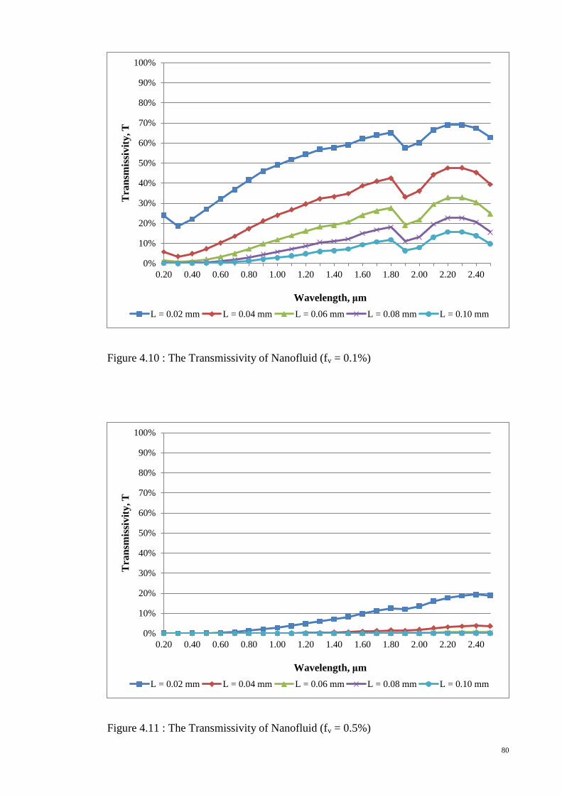
80
Figure 4.10 : The Transmissivity of Nanofluid (fv = 0.1%)
Figure 4.11 : The Transmissivity of Nanofluid (fv = 0.5%)
0%
10%
20%
30%
40%
50%
60%
70%
80%
90%
100%
0.20 0.40 0.60 0.80 1.00 1.20 1.40 1.60 1.80 2.00 2.20 2.40
Tra
nsm
issi
vit
y, T
Wavelength, μm
L = 0.02 mm L = 0.04 mm L = 0.06 mm L = 0.08 mm L = 0.10 mm
0%
10%
20%
30%
40%
50%
60%
70%
80%
90%
100%
0.20 0.40 0.60 0.80 1.00 1.20 1.40 1.60 1.80 2.00 2.20 2.40
Tra
nsm
issi
vit
y, T
Wavelength, μm
L = 0.02 mm L = 0.04 mm L = 0.06 mm L = 0.08 mm L = 0.10 mm
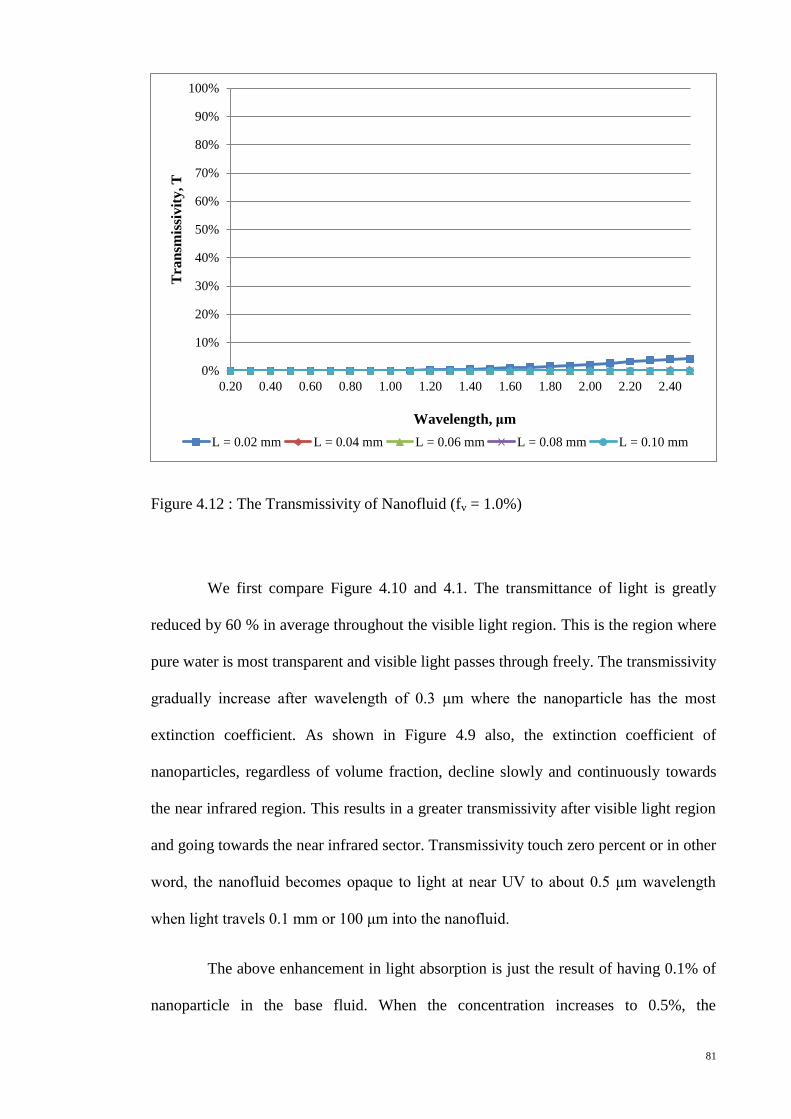
81
Figure 4.12 : The Transmissivity of Nanofluid (fv = 1.0%)
We first compare Figure 4.10 and 4.1. The transmittance of light is greatly
reduced by 60 % in average throughout the visible light region. This is the region where
pure water is most transparent and visible light passes through freely. The transmissivity
gradually increase after wavelength of 0.3 μm where the nanoparticle has the most
extinction coefficient. As shown in Figure 4.9 also, the extinction coefficient of
nanoparticles, regardless of volume fraction, decline slowly and continuously towards
the near infrared region. This results in a greater transmissivity after visible light region
and going towards the near infrared sector. Transmissivity touch zero percent or in other
word, the nanofluid becomes opaque to light at near UV to about 0.5 μm wavelength
when light travels 0.1 mm or 100 μm into the nanofluid.
The above enhancement in light absorption is just the result of having 0.1% of
nanoparticle in the base fluid. When the concentration increases to 0.5%, the
0%
10%
20%
30%
40%
50%
60%
70%
80%
90%
100%
0.20 0.40 0.60 0.80 1.00 1.20 1.40 1.60 1.80 2.00 2.20 2.40
Tra
nsm
issi
vit
y, T
Wavelength, μm
L = 0.02 mm L = 0.04 mm L = 0.06 mm L = 0.08 mm L = 0.10 mm
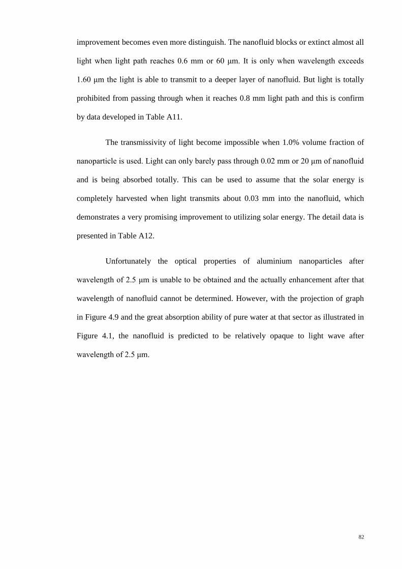
82
improvement becomes even more distinguish. The nanofluid blocks or extinct almost all
light when light path reaches 0.6 mm or 60 μm. It is only when wavelength exceeds
1.60 μm the light is able to transmit to a deeper layer of nanofluid. But light is totally
prohibited from passing through when it reaches 0.8 mm light path and this is confirm
by data developed in Table A11.
The transmissivity of light become impossible when 1.0% volume fraction of
nanoparticle is used. Light can only barely pass through 0.02 mm or 20 μm of nanofluid
and is being absorbed totally. This can be used to assume that the solar energy is
completely harvested when light transmits about 0.03 mm into the nanofluid, which
demonstrates a very promising improvement to utilizing solar energy. The detail data is
presented in Table A12.
Unfortunately the optical properties of aluminium nanoparticles after
wavelength of 2.5 μm is unable to be obtained and the actually enhancement after that
wavelength of nanofluid cannot be determined. However, with the projection of graph
in Figure 4.9 and the great absorption ability of pure water at that sector as illustrated in
Figure 4.1, the nanofluid is predicted to be relatively opaque to light wave after
wavelength of 2.5 μm.
83
Chapter 5: Conclusion and Future Recommendation
Solar energy, as the most vastly available energy and also supremely effective
in terms of energy conversion has been the most sought after. The most common solar
thermal collector utilizes black surface as radiant absorber but the efficiency is limited
to the effectiveness of the black surface and the transfer of thermal energy from the
black surface to the working fluid. After conducting this study, the thesis can bravely
conclude the following:
1. Direct Solar Collector uses nanofluids as volumetric absorber and is expected
to provide excellent optical properties and enhanced thermal transfer.
2. The extinction coefficient of nanofluid is evaluated with aluminium
nanoparticle as additive material and pure water as base fluid and nanoparticle
size and volume fraction as parameters. The particle sizes and volume fraction
studied are 1 nm to 10 nm and 0.1% to 8.0% respectively. Pure water appears
to be almost transparent to visible light but shows great absorption ability at
longer wavelength of about 2.6 μm onwards. Aluminium nanoparticle shows
very strong extinction coefficient at shorter wavelength and peak at 0.3 μm.
The extinction coefficient demonstrates a descending trend after that. Despite a
lower extinction coefficient at longer wavelength, aluminium nanoparticle is a
good match to pure water as it enhanced the light absorption ability of water at
the visible and shorter wavelength region.
3. The particle size shows minimal influence to the optical properties of nanofluid
while the extinction coefficient is linearly proportionate to volume fraction.
This is in common with the findings by Lenert (2010) and Tyagi (2008, 2009).
It is suggested that although the extinction coefficient of nanofluid is disregard
of the nanoparticle size, the nanoparticle size should be controlled to be below
84
20 nm in order for Rayleigh scattering to take place. On the other hand, the
volume fraction should be minimal after obtaining the desired optical
properties in order to avoid drawbacks like clogging and unstable suspension
of nanoparticles when incorporating nanofluid technology to Solar Collector.
The proposed nanoparticle size and volume fraction in this thesis is 10 nm and
below 2.0% respectively.
4. The transmissivity of light is compared between pure water (base fluid) and
nanofluid. The improvement is promising and with only 1.0% volume fraction,
the nanofluid is already almost opaque to light wave. Since volume fraction of
just 1.0% is already showing satisfactory improvement to solar absorption,
nanofluid with aluminium as nanoparticles and pure water as base fluid can be
concluded to be a good solution to Direct Solar Collector.
In the extension to this study, experiments to confirm the radiative properties
of the nanofluid should be carried out. The radiative properties for this nanofluid to light
wave exceeding wavelength of 2.5 μm can be determined by this way. Materials
showing promising radiative properties such as Single Wall Carbon Nanohorn
(SWCNH) (Mercatelli et al., 2011) can be integrated to future researches to investigate
the probability to be functioned as nano-additive. Further to this, base fluid with better
thermal properties and stability at high temperature can be studied to explore the
possibility of using nanofluid in solar collector of concentrating type. Last of all, the
researches in optical properties of nanofluid should take into consideration the
manufacturing process and cost of integration to the existing systems. Direct Solar
Collector has shown to be a very encouraging form of renewable energy and should be
further exploit to give human beings a better and cleaner future.
85
Bibliography
Abdelrahman, M., Fumeaux, P. & Suter, P. (1979). Study of Solid-Gas-Suspensions
Used For Direct Absorption of Concentrated Solar-Radiation. Solar Energy,
22(1), p. 45-48.
Anderson, B. (1977). Solar energy: fundamentals in building design. New York:
McGraw-Hill.
ASTM (American Society for Testing and Materials) Terrestrial Reference Spectra.
(2003). Reference Solar Spectral Irradiance: Air Mass 1.5. In ASTM G173-03.
Bar-Yosef, O. (2002). The upper Paleolithic revolution. Annual Review
of Anthropology, 31, 363-393.
Brewster, M.Q. (1992). Thermal radiative transfer and properties. Canada: John Wiley
& Sons.
Buongiorno, J. (2006). Convective transport in nanofluids. Journal of Heat Transfer,
128(3), 240-251.
Chaplin, M. (2011). Water Absorption Spectrum. In Water Structure and Science.
Retrieved 29 July 2011. From http://www.lsbu.ac.uk/water/vibrat.html#uv
Chen, C.W., Chiang, H.-P., Leung, P.T., & Tsai, D.P. (2008). Temperature dependence
of enhanced optical absorption and Raman Spectroscopy from Metallic
Nanoparticles. Solid State Communications, 148, 413-416.
Choi, U.S. (1995). Enhancing Thermal Conductivity of Fluids with Nanoparticles,
Developments and Applications of Non-NewtonianFlows, ASME FED 231/MD
(66), 99-103.

86
EGRE (Expert Group on Renewable Energy). (2005). Renewables 2005 Background
Report. In United Nations Department of Economic and Social Affairs
(UNDESA), Beijing International Renewable Energy Conference 2005
Background Report. Beijing, People‟s Republic of China. 7-8th
November 2005.
New York: United Nations.
Everett, B. (2004). Solar Thermal Energy. In Renewable Energy – Power for A
Sustainable Future (2nd
ed.) (pp. 17-64). New York: Oxford University Press.
Fan, X., Tan, J., Zhang, G., & Zhang, F. (2007). Isolation of carbon nanohorns
assemblies and their potential for intracellular delivery. Nanotechnology, 18,
195103, 1-6.
Four Peaks Technologies Inc. (2010). Solar In-Depth. In Solar Cell Central. Retrieved
27 July 2011. From http://solarcellcentral.com/physics_page.html
Francia, G. (1961). A new collector of solar radiant energy. UN Conf. New Sources
Energy, 4, 572.
Gleiter, H. (1989). Nanocrystalline Materials, Progress in Materials Science, 33(4),
223–315.
Hollands, K.G.T. (1965). Honeycomb devices in flat-plate solar collectors. Solar
Energy, 9(3), 159-164.
Hunt, A.J. (1978). Small Particle Heat Exchangers. Lawrence Berkeley Laboratory.
Horvath, H. (2009). Gustav Mie and the scattering and absorption of light by particles:
Historic developments and basics. Journal of Quantitative Spectroscopy &
Radiative Transfer, 110, 787-799.
87
Iijima, S., Yudaseka, M., Yamada, R., Bandow, S., Suenaga, K., Kokai, F., et al. (1999).
Nano-aggregrates of single-walled graphite carbon nano-horns. Chem Phys Lett,
309, 165-170.
International Energy Agency Renewable Energy Working Party. (2002). Renewable
Energy... into the mainstream, p. 9.
IAPWS (The International Association for the Properties of Water and Steam). (1997).
Release on the Refractive Index of Ordinary Water Substance as a Function of
Wavelength, Temperature and Pressure. Erlangen, Germany.
Kalogirou, S. (2003). The potential of solar industrial process heat applications.
Applied Energy, 76(4), 337–361.
Kalogirou, S.A. (2004). Solar Thermal Collectors and Applications. Progress in Energy
and Combustion Science, 30, 231-295.
Kalogirou, S.A., Eleftheriou, P., Lloyd, S., & Ward, J. (1994). Design and performance
characteristics of a parabolic-trough solarcollector system. Appl Energy, 47,
341–354.
Kameya, Y. & Hanamura, K. (2011). Enhancement of solar radiation absorption using
nanoparticle suspension. Solar Energy, 85, 299-307.
Karkanas, P., Shahack-Gross, R., Ayalon, A., Bar-Matthews, M., Barkai, R., Frumkin,
A., et al. (2007). Evidence for habitual use of fire at the end of the Lower
Paleolithic: Site-formation processes at Qesem Cave, Israel. Journal of Human
Evolution, 53 (2), 197-212.

88
Keblinski, P., Phillpot, S.R., Choi, S.U.S., & Eastman, J.A. (2002). Mechanisms of heat
flow in suspensions of nano-sized particles (nanofluids). International Journal of
Heat and Mass Transfer, 45, 855–863.
Khlebtsov, N.G., Trachuk, L.A., & Mel‟nikov, A.G. (2005). The effect of the size, shape,
and structure of metal nanoparticles on the dependence of their optical properties
on the refractive index of a disperse medium. Optics and Spectroscopy, 98(1), 77-
85.
Koo, J., & Kleinstreuer, C. (2005). Impact analysis of nanoparticle motion mechanisms
on the thermal conductivity of nanofluids. International Communication on Heat
and Mass Transfer, 32(9), 1111–1118.
Kou, L., Labrie, D., & Chylek, P. (1993). Refractive indices of water and ice in the
0.65 to 2.5 μm spectral range. Applied Optics, 32(19), 3531-3540.
Kreider, J.F., Kreith, F. (1977). Solar heating and cooling. New York: McGraw-Hill.
Kreith, F., Kreider, J.F. (1978). Principles of solar engineering. New York: McGraw-
Hill.
Kumar, N. (2008). Comprehensive Physics (7th
ed.). New Delhi: Laxmi Publications.
Lenert, A. (2010). Nanofluid-based Receivers for High-Temperature, High-flux Direct
Solar Collectors. M. Sc. Massachusetts Institute of Technology.
Lilienfeld, P. (2004). A Blue Sky History. Optics and Photonics News, June, 32-39.
Masruroh, N. A., Li, B. & Klemes, J. (2006). Life cycle analysis of solar thermal system
with thermochemical storage process, Renewable Energy, 31, 537-548.
Meinel, A.B., Meinel, M.P. (1976). Applied solar energy: an introduction. Reading,
MA: Addison-Wesley.

89
Mercatelli, L., Sani, E., Zaccanti, G., Martelli, F., Di Ninni, P., Barison, S., et al. (2011).
Absorption and scattering properties of carbon nanohorn-based nanofluid for
direct sunlight absorbers. Nanoscale Research Letters, 6, 282.
Meteonorm. (2008). Global irradiance World. In free meteonorm maps. Retrieved 21st
July 2011. From http://meteonorm.com/?id=32
Miller, F. J., and Koenigsdorff, R. W. (2000). Thermal modeling of a small-particle
solar central receiver, J. Solar Energy Eng., 122, 23-29.
Minardi, J. E., & Chunag, H. N. (1975). Performance of a black liquid flat-plate solar
collector, Solar Energy, 17, 179 -183.
Mishra, A., Srivastava, V.K., & Ram, S. (2008). Nonlinear variation of optical
absorption and rheological behavior with concentration in dispersed poly(vinyl
pyrrolidone) of small molecules in water. Journal of Molecular Liquids, 137, 58-
63.
Mishra, A., Ram, S., & Ghosh, G. (2009). Dynamic Light Scattering and Optical
Absorption in Biological Nanofluids of Gold Nanoparticles in Poly(vinyl
pyrrolidone) Molecules. J. Phys. Chem. C, 113, 6976-6982.
Mohr, P.J., Taylor, B.N., & Newell, D.B. (2011). "The 2010 CODATA Recommended
Values of the Fundamental Physical Constants" (Web Version 6.0). Retrieved 30
July 2011. From http://physics.nist.gov/constants
Molineaux, B., Lachal, B., & Gusian, O. (1994). Thermal analysis of five outdoor
swimming pools heated by unglazed solar collectors. Solar Energy, 53(1), 21–26.
Okujagu, C. U., & Adjepong, S. K. (1989). Performance of a simple flat-plate collector
at an equatorial location, Solar & Wind Tech., 6, 283-289.
90
Otanicar, T.P., Phelan, P.E., & Golden, J.S. (2009) Optical Properties of Liquids for
Direct Absorption Solar Thermal Energy Systems. Solar Energy, 83, 969-977.
Otanicar, T.P., Phelan, P.E., Prasher, R.S., Rosengarten, G., & Taylor, R.A. (2010).
Nanofluid-based Direct Absorption Solar Collector. Journal of Renewable and
Sustainable Energy, 2, 033102.
Pacheco, J.E. (2001). Demonstration of solar-generated electricity on demand: The
Solar Two project. Journal of Solar Energy Engineering-Transactions of the
ASME, 123(1), 5-5.
Pak, B.C., & Cho, I.Y. (1998). Hydrodynamic and heat transfer study of dispersed
fluids with sub-micron metallic oxide particles. Experimental Heat Transfer, 11,
151–170.
Pope, R.M., & Fry, E.S. (1997). Absorption spectrum (380 – 700 nm) of pure water. II.
Integrating cavity measurements. Applied Optics, 36(33), 8710-8723.
REN21 (Renewable Energy Policy Network in the 21st Century). (2011). Renewables
2011 – Global Status Report, p.11.
Saidur, R., Leong, K.Y., & Mohammad, H.A. (2011). A review on applications and
challenges of nanofluids. Renewable and Sustainable Energy Reviews, 15, 1646-
1668.
Sani, E., Barison, S., Pagura, C., Mercatelli, L., Sansoni, P., Fontani, D., et al. (2010).
Carbon nanohorns-based nanofluids as direct sunlight absorbers. Optics Express,
18(5), 5179-5187.
Serrano, E., Rus, G., & Martínez, J.G. (2009). Nanotechnology for sustainable energy.
Renewable and Sustainable Energy Reviews, 13, 2373-2384.
91
Smith, D.Y., Shiles, E. & Inokuti, M. (1985). The Optical Properties of Metallic
Aluminum. In E.D. Palik, ed. 1998. Handbook of optical constants of solids,
Volume 5. London: Academic Press Limited.
Smith, G.H. (2006). Camera Lenses: from Box Camera to Digital. Washington: The
International Society of Optical Engineering.
Soltau, H. (1992). Testing the thermal performance of uncovered solar collectors. Solar
Energy, 49(4), 263–272.
Sømensen, B. (2011). Renewable Energy (4th
ed.). Oxford: Academic Press.
Tester, J. W., Drake, E. M., Golay, M. W., Driscoll, M. J., & Peters, W. A. (2005).
Sustainable energy: Choosing among options, MIT Press, MA, 64-74.
Twidell, J. & Weir, A.D. (2006). Renewable Energy Resources (2nd
ed.). New York:
Taylor & Francis.
Tyagi, H. (2008) Radiative and Combustion Properties of Nanoparticles-Laden Liquid,
Ph. D. Arizona State University.
Tyagi, H., Phelan, P., & Prasher, R. (2009). Predicted Efficiency of a Low-temperature
Nanofluid-based Direct Absorption Solar Collector. Journal of Solar Energy
Engineering, 131, 041004-1 - 041004-7.
US DOE (United States Department of Energy). (2010a). Overview. In International
Energy Outlook 2010. Retrieved 17 July 2011. From
http://www.eia.gov/oiaf/ieo/electricity.html
US DOE (United States Department of Energy). (2010b). Electricity Supply by Energy
Source. In International Energy Outlook 2010. Retrieved 17 July 2011. From
http://www.eia.gov/oiaf/ieo/electricity.html
92
US EPA (United States Environmental Protection Agency). (2011a). Nitrogen Dioxide.
In Six Common Pollutants. Retrieved 17 July 2011. From
http://www.epa.gov/air/nitrogenoxides/
US EPA (United States Environmental Protection Agency). (2011b). Health. In
Nitrogen Dioxide. Retrieved 17 July 2011. From
http://www.epa.gov/airquality/nitrogenoxides/health.html
Van de Hulst, H.C. (1981). Light scattering by small particles. New York: Dover
Publications.
Weiss, W., & Mauthner, F. (2011). Solar Heat Worldwide: Markets and Contribution to
the Energy Supply 2009, prepared for IEA Solar Heating and Cooling Programme.
Wikibooks. (2011). Energy from the Sun. In High School Earth Science/Energy in the
Atmosphere. Retrieved 7 August 2011. From
http://en.wikibooks.org/wiki/High_School_Earth_Science/Energy_in_the_Atmosp
here
Wikipedia. (2011a). Objectives. In Kyoto Protocol. Retrieved 17 July, 2011. From
http://en.wikipedia.org/wiki/Kyoto_protocol
Wikipedia, (2011b). Visible Spectrum. Retrieved 30 July, 2011. From
http://en.wikipedia.org/wiki/Visible_spectrum#cite_ref-0.
Wikipedia. (2011c). Spectral colors. In Visible Spectrum. Retrieved 30 July, 2011. From
http://en.wikipedia.org/wiki/Visible_spectrum#Spectral_colors.
Wikipedia. (2011e). Light Scattering. Retrieved 31 July, 2011. From
http://en.wikipedia.org/wiki/Light_scattering

93
Winter, F. (1994). Twenty-year progress report on the copper development association
do-it-yourself solar swimming pool heating manual and on the associated
prototype heater. Solar Energy, 53(1), 33–36.
Wrangham, R. W., Jones, J. H., Laden, G., Pilbeam, D., Conklin-Brittain, N. (1999).
The raw and the stolen: Cooking and the ecology of human origins. Current
Anthropology, 40(5), 567-594.
Xuan, Y., & Li, Q. (2000). Heat transfer enhancement of nanofluids. International
Journal of Heat and Fluid Flow, 21, 58–64.

94
Appendix 1
Table A1 : Pure Water Refractive index, n and Absorption index, k, as Function of
Wavelength, λ (Irvine and Pollack, 1968 cited in Brewster, 1992, p.507)
λ (μm) n k
λ (μm) n k
0.20 1.4240 1.300E-07
2.00 1.3040 1.082E-03
0.30 1.3590 3.600E-08
2.10 1.3000 4.345E-04
0.40 1.3430 3.000E-09
2.20 1.2930 2.800E-04
0.50 1.3360 8.000E-10
2.25 1.2920 3.040E-04
0.60 1.3320 7.000E-09
2.30 1.2860 4.210E-04
0.70 1.3300 3.300E-08
2.40 1.2760 8.020E-04
0.80 1.3280 1.340E-07
2.50 1.2460 1.651E-03
0.90 1.3280 4.800E-07
2.60 1.1800 2.048E-03
1.00 1.3260 2.820E-06
2.70 1.1340 5.049E-03
1.10 1.3240 1.660E-06
2.75 1.1330 2.401E-02
1.20 1.3230 9.740E-06
2.80 1.2320 9.361E-02
1.30 1.3210 1.117E-05 2.90 1.3100 2.435E-01
1.40 1.3200 1.448E-04
3.00 1.3510 2.586E-01
1.50 1.3180 2.065E-04
3.10 1.4260 1.828E-01
1.60 1.3160 7.890E-05
3.20 1.5090 9.422E-02
1.70 1.3150 6.970E-05
3.30 1.4700 4.333E-02
1.80 1.3120 1.146E-04
3.40 1.4490 1.888E-02
1.90 1.3090 1.217E-03
3.50 1.4230 9.300E-03
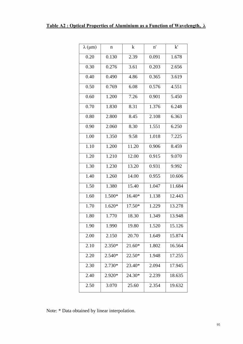
95
Table A2 : Optical Properties of Aluminium as a Function of Wavelength, λ
λ (μm) n k n' k'
0.20 0.130 2.39 0.091 1.678
0.30 0.276 3.61 0.203 2.656
0.40 0.490 4.86 0.365 3.619
0.50 0.769 6.08 0.576 4.551
0.60 1.200 7.26 0.901 5.450
0.70 1.830 8.31 1.376 6.248
0.80 2.800 8.45 2.108 6.363
0.90 2.060 8.30 1.551 6.250
1.00 1.350 9.58 1.018 7.225
1.10 1.200 11.20 0.906 8.459
1.20 1.210 12.00 0.915 9.070
1.30 1.230 13.20 0.931 9.992
1.40 1.260 14.00 0.955 10.606
1.50 1.380 15.40 1.047 11.684
1.60 1.500* 16.40* 1.138 12.443
1.70 1.620* 17.50* 1.229 13.278
1.80 1.770 18.30 1.349 13.948
1.90 1.990 19.80 1.520 15.126
2.00 2.150 20.70 1.649 15.874
2.10 2.350* 21.60* 1.802 16.564
2.20 2.540* 22.50* 1.948 17.255
2.30 2.730* 23.40* 2.094 17.945
2.40 2.920* 24.30* 2.239 18.635
2.50 3.070 25.60 2.354 19.632
Note: * Data obtained by linear interpolation.
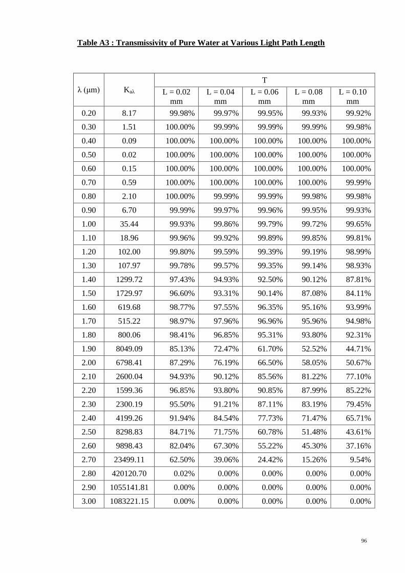
96
Table A3 : Transmissivity of Pure Water at Various Light Path Length
λ (μm) Kaλ
T
L = 0.02
mm
L = 0.04
mm
L = 0.06
mm
L = 0.08
mm
L = 0.10
mm
0.20 8.17 99.98% 99.97% 99.95% 99.93% 99.92%
0.30 1.51 100.00% 99.99% 99.99% 99.99% 99.98%
0.40 0.09 100.00% 100.00% 100.00% 100.00% 100.00%
0.50 0.02 100.00% 100.00% 100.00% 100.00% 100.00%
0.60 0.15 100.00% 100.00% 100.00% 100.00% 100.00%
0.70 0.59 100.00% 100.00% 100.00% 100.00% 99.99%
0.80 2.10 100.00% 99.99% 99.99% 99.98% 99.98%
0.90 6.70 99.99% 99.97% 99.96% 99.95% 99.93%
1.00 35.44 99.93% 99.86% 99.79% 99.72% 99.65%
1.10 18.96 99.96% 99.92% 99.89% 99.85% 99.81%
1.20 102.00 99.80% 99.59% 99.39% 99.19% 98.99%
1.30 107.97 99.78% 99.57% 99.35% 99.14% 98.93%
1.40 1299.72 97.43% 94.93% 92.50% 90.12% 87.81%
1.50 1729.97 96.60% 93.31% 90.14% 87.08% 84.11%
1.60 619.68 98.77% 97.55% 96.35% 95.16% 93.99%
1.70 515.22 98.97% 97.96% 96.96% 95.96% 94.98%
1.80 800.06 98.41% 96.85% 95.31% 93.80% 92.31%
1.90 8049.09 85.13% 72.47% 61.70% 52.52% 44.71%
2.00 6798.41 87.29% 76.19% 66.50% 58.05% 50.67%
2.10 2600.04 94.93% 90.12% 85.56% 81.22% 77.10%
2.20 1599.36 96.85% 93.80% 90.85% 87.99% 85.22%
2.30 2300.19 95.50% 91.21% 87.11% 83.19% 79.45%
2.40 4199.26 91.94% 84.54% 77.73% 71.47% 65.71%
2.50 8298.83 84.71% 71.75% 60.78% 51.48% 43.61%
2.60 9898.43 82.04% 67.30% 55.22% 45.30% 37.16%
2.70 23499.11 62.50% 39.06% 24.42% 15.26% 9.54%
2.80 420120.70 0.02% 0.00% 0.00% 0.00% 0.00%
2.90 1055141.81 0.00% 0.00% 0.00% 0.00% 0.00%
3.00 1083221.15 0.00% 0.00% 0.00% 0.00% 0.00%
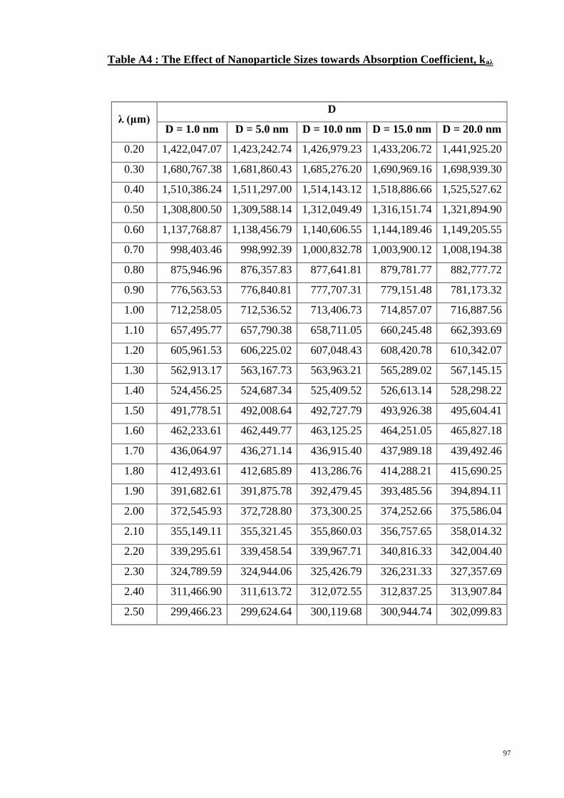
97
Table A4 : The Effect of Nanoparticle Sizes towards Absorption Coefficient, kaλ
λ (μm) D
D = 1.0 nm D = 5.0 nm D = 10.0 nm D = 15.0 nm D = 20.0 nm
0.20 1,422,047.07 1,423,242.74 1,426,979.23 1,433,206.72 1,441,925.20
0.30 1,680,767.38 1,681,860.43 1,685,276.20 1,690,969.16 1,698,939.30
0.40 1,510,386.24 1,511,297.00 1,514,143.12 1,518,886.66 1,525,527.62
0.50 1,308,800.50 1,309,588.14 1,312,049.49 1,316,151.74 1,321,894.90
0.60 1,137,768.87 1,138,456.79 1,140,606.55 1,144,189.46 1,149,205.55
0.70 998,403.46 998,992.39 1,000,832.78 1,003,900.12 1,008,194.38
0.80 875,946.96 876,357.83 877,641.81 879,781.77 882,777.72
0.90 776,563.53 776,840.81 777,707.31 779,151.48 781,173.32
1.00 712,258.05 712,536.52 713,406.73 714,857.07 716,887.56
1.10 657,495.77 657,790.38 658,711.05 660,245.48 662,393.69
1.20 605,961.53 606,225.02 607,048.43 608,420.78 610,342.07
1.30 562,913.17 563,167.73 563,963.21 565,289.02 567,145.15
1.40 524,456.25 524,687.34 525,409.52 526,613.14 528,298.22
1.50 491,778.51 492,008.64 492,727.79 493,926.38 495,604.41
1.60 462,233.61 462,449.77 463,125.25 464,251.05 465,827.18
1.70 436,064.97 436,271.14 436,915.40 437,989.18 439,492.46
1.80 412,493.61 412,685.89 413,286.76 414,288.21 415,690.25
1.90 391,682.61 391,875.78 392,479.45 393,485.56 394,894.11
2.00 372,545.93 372,728.80 373,300.25 374,252.66 375,586.04
2.10 355,149.11 355,321.45 355,860.03 356,757.65 358,014.32
2.20 339,295.61 339,458.54 339,967.71 340,816.33 342,004.40
2.30 324,789.59 324,944.06 325,426.79 326,231.33 327,357.69
2.40 311,466.90 311,613.72 312,072.55 312,837.25 313,907.84
2.50 299,466.23 299,624.64 300,119.68 300,944.74 302,099.83

98
Table 5 : The Effect of Nanoparticle Sizes towards Scattering Coefficient, ksλ
λ (μm) D
D = 1.0 nm D = 5.0 nm D = 10.0 nm D = 15.0 nm D = 20.0 nm
0.20 2.37 296.87 2,374.97 8,015.52 18,999.76
0.30 0.42 53.06 424.48 1,432.62 3,395.85
0.40 0.10 12.57 100.55 339.35 804.37
0.50 0.02 2.56 20.52 69.24 164.12
0.60 0.00 0.07 0.54 1.82 4.32
0.70 0.00 0.43 3.42 11.53 27.33
0.80 0.01 1.36 10.87 36.70 86.98
0.90 0.00 0.30 2.42 8.17 19.36
1.00 0.00 0.00 0.00 0.01 0.02
1.10 0.00 0.01 0.04 0.14 0.34
1.20 0.00 0.00 0.02 0.08 0.20
1.30 0.00 0.00 0.01 0.04 0.09
1.40 0.00 0.00 0.00 0.01 0.03
1.50 0.00 0.00 0.00 0.01 0.02
1.60 0.00 0.00 0.02 0.06 0.15
1.70 0.00 0.00 0.04 0.13 0.32
1.80 0.00 0.01 0.07 0.23 0.55
1.90 0.00 0.01 0.11 0.37 0.88
2.00 0.00 0.02 0.13 0.44 1.03
2.10 0.00 0.02 0.15 0.50 1.18
2.20 0.00 0.02 0.15 0.52 1.24
2.30 0.00 0.02 0.16 0.53 1.25
2.40 0.00 0.02 0.15 0.52 1.23
2.50 0.00 0.02 0.14 0.49 1.16
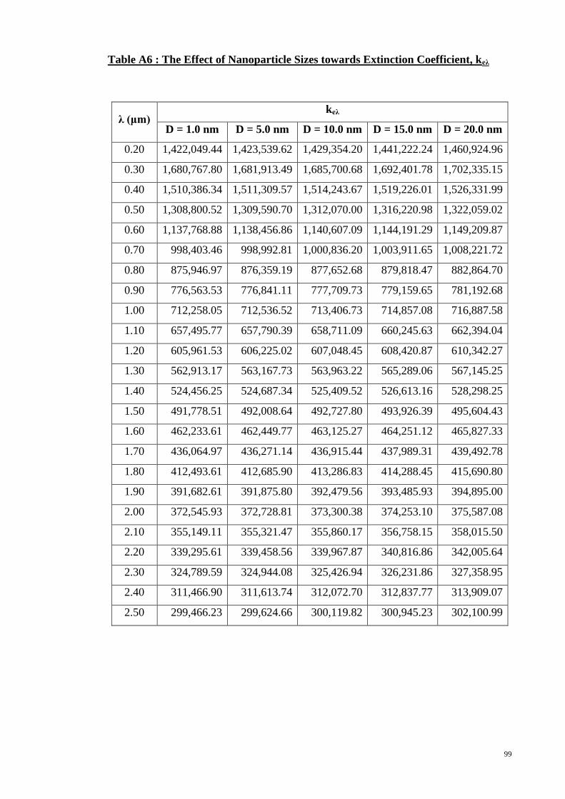
99
Table A6 : The Effect of Nanoparticle Sizes towards Extinction Coefficient, keλ
λ (μm) keλ
D = 1.0 nm D = 5.0 nm D = 10.0 nm D = 15.0 nm D = 20.0 nm
0.20 1,422,049.44 1,423,539.62 1,429,354.20 1,441,222.24 1,460,924.96
0.30 1,680,767.80 1,681,913.49 1,685,700.68 1,692,401.78 1,702,335.15
0.40 1,510,386.34 1,511,309.57 1,514,243.67 1,519,226.01 1,526,331.99
0.50 1,308,800.52 1,309,590.70 1,312,070.00 1,316,220.98 1,322,059.02
0.60 1,137,768.88 1,138,456.86 1,140,607.09 1,144,191.29 1,149,209.87
0.70 998,403.46 998,992.81 1,000,836.20 1,003,911.65 1,008,221.72
0.80 875,946.97 876,359.19 877,652.68 879,818.47 882,864.70
0.90 776,563.53 776,841.11 777,709.73 779,159.65 781,192.68
1.00 712,258.05 712,536.52 713,406.73 714,857.08 716,887.58
1.10 657,495.77 657,790.39 658,711.09 660,245.63 662,394.04
1.20 605,961.53 606,225.02 607,048.45 608,420.87 610,342.27
1.30 562,913.17 563,167.73 563,963.22 565,289.06 567,145.25
1.40 524,456.25 524,687.34 525,409.52 526,613.16 528,298.25
1.50 491,778.51 492,008.64 492,727.80 493,926.39 495,604.43
1.60 462,233.61 462,449.77 463,125.27 464,251.12 465,827.33
1.70 436,064.97 436,271.14 436,915.44 437,989.31 439,492.78
1.80 412,493.61 412,685.90 413,286.83 414,288.45 415,690.80
1.90 391,682.61 391,875.80 392,479.56 393,485.93 394,895.00
2.00 372,545.93 372,728.81 373,300.38 374,253.10 375,587.08
2.10 355,149.11 355,321.47 355,860.17 356,758.15 358,015.50
2.20 339,295.61 339,458.56 339,967.87 340,816.86 342,005.64
2.30 324,789.59 324,944.08 325,426.94 326,231.86 327,358.95
2.40 311,466.90 311,613.74 312,072.70 312,837.77 313,909.07
2.50 299,466.23 299,624.66 300,119.82 300,945.23 302,100.99
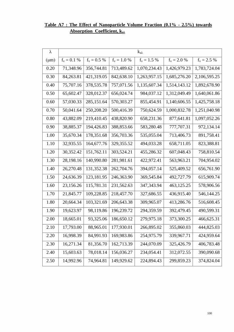
100
Table A7 : The Effect of Nanoparticle Volume Fraction (0.1% - 2.5%) towards
Absorption Coefficient, kaλ
λ
(μm)
kaλ
fv = 0.1 % fv = 0.5 % fv = 1.0 % fv = 1.5 % fv = 2.0 % fv = 2.5 %
0.20 71,348.96 356,744.81 713,489.62 1,070,234.43 1,426,979.23 1,783,724.04
0.30 84,263.81 421,319.05 842,638.10 1,263,957.15 1,685,276.20 2,106,595.25
0.40 75,707.16 378,535.78 757,071.56 1,135,607.34 1,514,143.12 1,892,678.90
0.50 65,602.47 328,012.37 656,024.74 984,037.12 1,312,049.49 1,640,061.86
0.60 57,030.33 285,151.64 570,303.27 855,454.91 1,140,606.55 1,425,758.18
0.70 50,041.64 250,208.20 500,416.39 750,624.59 1,000,832.78 1,251,040.98
0.80 43,882.09 219,410.45 438,820.90 658,231.36 877,641.81 1,097,052.26
0.90 38,885.37 194,426.83 388,853.66 583,280.48 777,707.31 972,134.14
1.00 35,670.34 178,351.68 356,703.36 535,055.04 713,406.73 891,758.41
1.10 32,935.55 164,677.76 329,355.52 494,033.28 658,711.05 823,388.81
1.20 30,352.42 151,762.11 303,524.21 455,286.32 607,048.43 758,810.54
1.30 28,198.16 140,990.80 281,981.61 422,972.41 563,963.21 704,954.02
1.40 26,270.48 131,352.38 262,704.76 394,057.14 525,409.52 656,761.90
1.50 24,636.39 123,181.95 246,363.90 369,545.84 492,727.79 615,909.74
1.60 23,156.26 115,781.31 231,562.63 347,343.94 463,125.25 578,906.56
1.70 21,845.77 109,228.85 218,457.70 327,686.55 436,915.40 546,144.25
1.80 20,664.34 103,321.69 206,643.38 309,965.07 413,286.76 516,608.45
1.90 19,623.97 98,119.86 196,239.72 294,359.59 392,479.45 490,599.31
2.00 18,665.01 93,325.06 186,650.12 279,975.18 373,300.25 466,625.31
2.10 17,793.00 88,965.01 177,930.01 266,895.02 355,860.03 444,825.03
2.20 16,998.39 84,991.93 169,983.86 254,975.79 339,967.71 424,959.64
2.30 16,271.34 81,356.70 162,713.39 244,070.09 325,426.79 406,783.48
2.40 15,603.63 78,018.14 156,036.27 234,054.41 312,072.55 390,090.68
2.50 14,992.96 74,964.81 149,929.62 224,894.43 299,859.23 374,824.04

101
Table A7a : The Effect of Nanoparticle Volume Fraction (1.0% - 8.0%) towards Absorption Coefficient, kaλ
λ (μm) kaλ
fv = 1.0 % fv = 2.0 % fv = 3.0 % fv = 4.0 % fv = 5.0 % fv = 6.0 % fv = 7.0 % fv = 8.0 %
0.20 713,489.62 1,426,979.23 2,140,468.85 2,853,958.47 3,567,448.09 4,280,937.70 4,994,427.32 5,707,916.94
0.30 842,638.10 1,685,276.20 2,527,914.30 3,370,552.40 4,213,190.50 5,055,828.61 5,898,466.71 6,741,104.81
0.40 757,071.56 1,514,143.12 2,271,214.68 3,028,286.24 3,785,357.80 4,542,429.37 5,299,500.93 6,056,572.49
0.50 656,024.74 1,312,049.49 1,968,074.23 2,624,098.98 3,280,123.72 3,936,148.46 4,592,173.21 5,248,197.95
0.60 570,303.27 1,140,606.55 1,710,909.82 2,281,213.09 2,851,516.36 3,421,819.64 3,992,122.91 4,562,426.18
0.70 500,416.39 1,000,832.78 1,501,249.18 2,001,665.57 2,502,081.96 3,002,498.35 3,502,914.75 4,003,331.14
0.80 438,820.90 877,641.81 1,316,462.71 1,755,283.62 2,194,104.52 2,632,925.43 3,071,746.33 3,510,567.24
0.90 388,853.66 777,707.31 1,166,560.97 1,555,414.62 1,944,268.28 2,333,121.93 2,721,975.59 3,110,829.25
1.00 356,703.36 713,406.73 1,070,110.09 1,426,813.45 1,783,516.81 2,140,220.18 2,496,923.54 2,853,626.90
1.10 329,355.52 658,711.05 988,066.57 1,317,422.09 1,646,777.62 1,976,133.14 2,305,488.66 2,634,844.19
1.20 303,524.21 607,048.43 910,572.64 1,214,096.86 1,517,621.07 1,821,145.28 2,124,669.50 2,428,193.71
1.30 281,981.61 563,963.21 845,944.82 1,127,926.43 1,409,908.03 1,691,889.64 1,973,871.24 2,255,852.85
1.40 262,704.76 525,409.52 788,114.28 1,050,819.04 1,313,523.79 1,576,228.55 1,838,933.31 2,101,638.07
1.50 246,363.90 492,727.79 739,091.69 985,455.59 1,231,819.48 1,478,183.38 1,724,547.28 1,970,911.17
1.60 231,562.63 463,125.25 694,687.88 926,250.50 1,157,813.13 1,389,375.75 1,620,938.38 1,852,501.01
1.70 218,457.70 436,915.40 655,373.10 873,830.81 1,092,288.51 1,310,746.21 1,529,203.91 1,747,661.61
1.80 206,643.38 413,286.76 619,930.14 826,573.52 1,033,216.90 1,239,860.28 1,446,503.66 1,653,147.04
1.90 196,239.72 392,479.45 588,719.17 784,958.90 981,198.62 1,177,438.34 1,373,678.07 1,569,917.79
2.00 186,650.12 373,300.25 559,950.37 746,600.49 933,250.62 1,119,900.74 1,306,550.86 1,493,200.99
2.10 177,930.01 355,860.03 533,790.04 711,720.05 889,650.06 1,067,580.08 1,245,510.09 1,423,440.10
2.20 169,983.86 339,967.71 509,951.57 679,935.43 849,919.29 1,019,903.14 1,189,887.00 1,359,870.86
2.30 162,713.39 325,426.79 488,140.18 650,853.58 813,566.97 976,280.36 1,138,993.76 1,301,707.15
2.40 156,036.27 312,072.55 468,108.82 624,145.09 780,181.36 936,217.64 1,092,253.91 1,248,290.18
2.50 149,929.62 299,859.23 449,788.85 599,718.47 749,648.08 899,577.70 1,049,507.32 1,199,436.94

102
Table 4.8 : The Effect of Nanoparticle Volume Fraction (0.1% - 2.5%) towards
Scattering Coefficient, ksλ
λ (μm) ksλ
fv = 0.1 % fv = 0.5 % fv = 1.0 % fv = 1.5 % fv = 2.0 % fv = 2.5 %
0.20 118.75 593.74 1,187.48 1,781.23 2,374.97 2,968.71
0.30 21.22 106.12 212.24 318.36 424.48 530.60
0.40 5.03 25.14 50.27 75.41 100.55 125.68
0.50 1.03 5.13 10.26 15.39 20.52 25.64
0.60 0.03 0.13 0.27 0.40 0.54 0.67
0.70 0.17 0.85 1.71 2.56 3.42 4.27
0.80 0.54 2.72 5.44 8.15 10.87 13.59
0.90 0.12 0.60 1.21 1.81 2.42 3.02
1.00 0.00 0.00 0.00 0.00 0.00 0.00
1.10 0.00 0.01 0.02 0.03 0.04 0.05
1.20 0.00 0.01 0.01 0.02 0.02 0.03
1.30 0.00 0.00 0.01 0.01 0.01 0.01
1.40 0.00 0.00 0.00 0.00 0.00 0.00
1.50 0.00 0.00 0.00 0.00 0.00 0.00
1.60 0.00 0.00 0.01 0.01 0.02 0.02
1.70 0.00 0.01 0.02 0.03 0.04 0.05
1.80 0.00 0.02 0.03 0.05 0.07 0.09
1.90 0.01 0.03 0.06 0.08 0.11 0.14
2.00 0.01 0.03 0.06 0.10 0.13 0.16
2.10 0.01 0.04 0.07 0.11 0.15 0.18
2.20 0.01 0.04 0.08 0.12 0.15 0.19
2.30 0.01 0.04 0.08 0.12 0.16 0.20
2.40 0.01 0.04 0.08 0.12 0.15 0.19
2.50 0.01 0.04 0.07 0.11 0.14 0.18

103
Table 4.8a : The Effect of Nanoparticle Volume Fraction (2.0% - 8.0%) towards
Scattering Coefficient, ksλ
λ
(μm)
ksλ
fv =
2.0 %
fv =
3.0 %
fv =
4.0 %
fv =
5.0 %
fv =
6.0 %
fv =
7.0 %
fv =
8.0 %
0.20 2,374.97 3,562.45 4,749.94 5,937.42 7,124.91 8,312.39 9,499.88
0.30 424.48 636.72 848.96 1,061.20 1,273.44 1,485.68 1,697.92
0.40 100.55 150.82 201.09 251.37 301.64 351.91 402.19
0.50 20.52 30.77 41.03 51.29 61.55 71.80 82.06
0.60 0.54 0.81 1.08 1.35 1.62 1.89 2.16
0.70 3.42 5.13 6.83 8.54 10.25 11.96 13.67
0.80 10.87 16.31 21.75 27.18 32.62 38.06 43.49
0.90 2.42 3.63 4.84 6.05 7.26 8.47 9.68
1.00 0.00 0.00 0.00 0.01 0.01 0.01 0.01
1.10 0.04 0.06 0.09 0.11 0.13 0.15 0.17
1.20 0.02 0.04 0.05 0.06 0.07 0.09 0.10
1.30 0.01 0.02 0.02 0.03 0.04 0.04 0.05
1.40 0.00 0.01 0.01 0.01 0.01 0.01 0.02
1.50 0.00 0.00 0.01 0.01 0.01 0.01 0.01
1.60 0.02 0.03 0.04 0.05 0.06 0.07 0.08
1.70 0.04 0.06 0.08 0.10 0.12 0.14 0.16
1.80 0.07 0.10 0.14 0.17 0.21 0.24 0.27
1.90 0.11 0.17 0.22 0.28 0.33 0.39 0.44
2.00 0.13 0.19 0.26 0.32 0.39 0.45 0.52
2.10 0.15 0.22 0.29 0.37 0.44 0.51 0.59
2.20 0.15 0.23 0.31 0.39 0.46 0.54 0.62
2.30 0.16 0.23 0.31 0.39 0.47 0.55 0.63
2.40 0.15 0.23 0.31 0.38 0.46 0.54 0.62
2.50 0.14 0.22 0.29 0.36 0.43 0.51 0.58

104
Table A9 : The Effect of Nanoparticle Volume Fractions towards Extinction Coefficient, keλ
λ (μm) ksλ
fv = 1.0 % fv = 2.0 % fv = 2.5 % fv = 3.0 % fv = 4.0 % fv = 5.0 % fv = 6.0 % fv = 7.0 % fv = 8.0 %
0.20 714,677.10 1,429,354.20 1,786,692.76 2,144,031.31 2,858,708.41 3,573,385.51 4,288,062.61 5,002,739.71 5,717,416.82
0.30 842,850.34 1,685,700.68 2,107,125.85 2,528,551.02 3,371,401.37 4,214,251.71 5,057,102.05 5,899,952.39 6,742,802.73
0.40 757,121.83 1,514,243.67 1,892,804.59 2,271,365.50 3,028,487.34 3,785,609.17 4,542,731.01 5,299,852.84 6,056,974.67
0.50 656,035.00 1,312,070.00 1,640,087.50 1,968,105.01 2,624,140.01 3,280,175.01 3,936,210.01 4,592,245.01 5,248,280.01
0.60 570,303.54 1,140,607.09 1,425,758.86 1,710,910.63 2,281,214.17 2,851,517.71 3,421,821.26 3,992,124.80 4,562,428.34
0.70 500,418.10 1,000,836.20 1,251,045.25 1,501,254.30 2,001,672.40 2,502,090.50 3,002,508.61 3,502,926.71 4,003,344.81
0.80 438,826.34 877,652.68 1,097,065.85 1,316,479.02 1,755,305.36 2,194,131.71 2,632,958.05 3,071,784.39 3,510,610.73
0.90 388,854.87 777,709.73 972,137.16 1,166,564.60 1,555,419.46 1,944,274.33 2,333,129.19 2,721,984.06 3,110,838.92
1.00 356,703.36 713,406.73 891,758.41 1,070,110.09 1,426,813.46 1,783,516.82 2,140,220.18 2,496,923.55 2,853,626.91
1.10 329,355.54 658,711.09 823,388.86 988,066.63 1,317,422.18 1,646,777.72 1,976,133.27 2,305,488.81 2,634,844.36
1.20 303,524.23 607,048.45 758,810.57 910,572.68 1,214,096.91 1,517,621.13 1,821,145.36 2,124,669.59 2,428,193.81
1.30 281,981.61 563,963.22 704,954.03 845,944.84 1,127,926.45 1,409,908.06 1,691,889.67 1,973,871.29 2,255,852.90
1.40 262,704.76 525,409.52 656,761.90 788,114.28 1,050,819.04 1,313,523.80 1,576,228.56 1,838,933.33 2,101,638.09
1.50 246,363.90 492,727.80 615,909.75 739,091.69 985,455.59 1,231,819.49 1,478,183.39 1,724,547.29 1,970,911.19
1.60 231,562.64 463,125.27 578,906.59 694,687.91 926,250.54 1,157,813.18 1,389,375.81 1,620,938.45 1,852,501.08
1.70 218,457.72 436,915.44 546,144.30 655,373.16 873,830.88 1,092,288.61 1,310,746.33 1,529,204.05 1,747,661.77
1.80 206,643.41 413,286.83 516,608.54 619,930.24 826,573.66 1,033,217.07 1,239,860.48 1,446,503.90 1,653,147.31
1.90 196,239.78 392,479.56 490,599.45 588,719.34 784,959.12 981,198.90 1,177,438.68 1,373,678.46 1,569,918.23
2.00 186,650.19 373,300.38 466,625.47 559,950.56 746,600.75 933,250.94 1,119,901.13 1,306,551.31 1,493,201.50
2.10 177,930.09 355,860.17 444,825.22 533,790.26 711,720.34 889,650.43 1,067,580.52 1,245,510.60 1,423,440.69
2.20 169,983.93 339,967.87 424,959.84 509,951.80 679,935.74 849,919.67 1,019,903.61 1,189,887.54 1,359,871.48
2.30 162,713.47 325,426.94 406,783.68 488,140.42 650,853.89 813,567.36 976,280.83 1,138,994.30 1,301,707.78
2.40 156,036.35 312,072.70 390,090.87 468,109.05 624,145.40 780,181.75 936,218.10 1,092,254.45 1,248,290.80
2.50 149,929.69 299,859.38 374,824.22 449,789.07 599,718.76 749,648.45 899,578.14 1,049,507.83 1,199,437.51
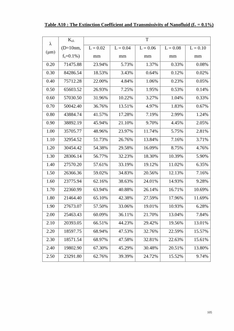
105
Table A10 : The Extinction Coefficient and Transmissivity of Nanofluid (fv = 0.1%)
λ
(μm)
Keλ
(D=10nm,
fv=0.1%)
T
L = 0.02
mm
L = 0.04
mm
L = 0.06
mm
L = 0.08
mm
L = 0.10
mm
0.20 71475.88 23.94% 5.73% 1.37% 0.33% 0.08%
0.30 84286.54 18.53% 3.43% 0.64% 0.12% 0.02%
0.40 75712.28 22.00% 4.84% 1.06% 0.23% 0.05%
0.50 65603.52 26.93% 7.25% 1.95% 0.53% 0.14%
0.60 57030.50 31.96% 10.22% 3.27% 1.04% 0.33%
0.70 50042.40 36.76% 13.51% 4.97% 1.83% 0.67%
0.80 43884.74 41.57% 17.28% 7.19% 2.99% 1.24%
0.90 38892.19 45.94% 21.10% 9.70% 4.45% 2.05%
1.00 35705.77 48.96% 23.97% 11.74% 5.75% 2.81%
1.10 32954.52 51.73% 26.76% 13.84% 7.16% 3.71%
1.20 30454.42 54.38% 29.58% 16.09% 8.75% 4.76%
1.30 28306.14 56.77% 32.23% 18.30% 10.39% 5.90%
1.40 27570.20 57.61% 33.19% 19.12% 11.02% 6.35%
1.50 26366.36 59.02% 34.83% 20.56% 12.13% 7.16%
1.60 23775.94 62.16% 38.63% 24.01% 14.93% 9.28%
1.70 22360.99 63.94% 40.88% 26.14% 16.71% 10.69%
1.80 21464.40 65.10% 42.38% 27.59% 17.96% 11.69%
1.90 27673.07 57.50% 33.06% 19.01% 10.93% 6.28%
2.00 25463.43 60.09% 36.11% 21.70% 13.04% 7.84%
2.10 20393.05 66.51% 44.23% 29.42% 19.56% 13.01%
2.20 18597.75 68.94% 47.53% 32.76% 22.59% 15.57%
2.30 18571.54 68.97% 47.58% 32.81% 22.63% 15.61%
2.40 19802.90 67.30% 45.29% 30.48% 20.51% 13.80%
2.50 23291.80 62.76% 39.39% 24.72% 15.52% 9.74%
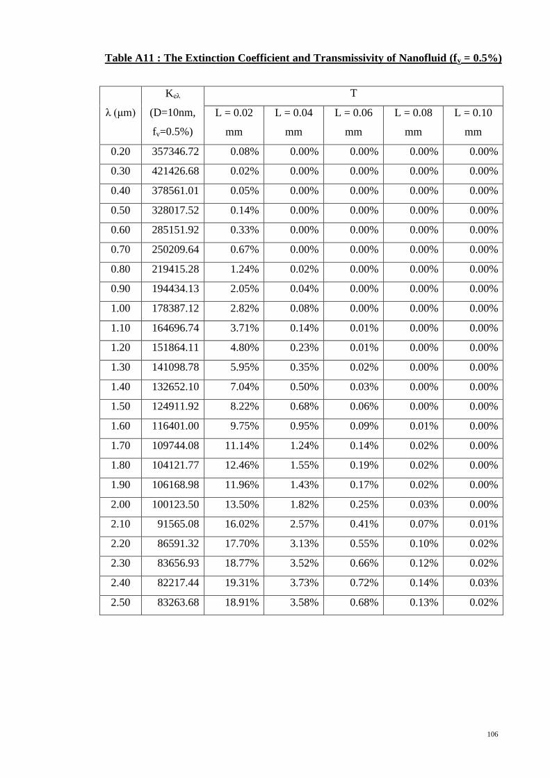
106
Table A11 : The Extinction Coefficient and Transmissivity of Nanofluid (fv = 0.5%)
λ (μm)
Keλ
(D=10nm,
fv=0.5%)
T
L = 0.02
mm
L = 0.04
mm
L = 0.06
mm
L = 0.08
mm
L = 0.10
mm
0.20 357346.72 0.08% 0.00% 0.00% 0.00% 0.00%
0.30 421426.68 0.02% 0.00% 0.00% 0.00% 0.00%
0.40 378561.01 0.05% 0.00% 0.00% 0.00% 0.00%
0.50 328017.52 0.14% 0.00% 0.00% 0.00% 0.00%
0.60 285151.92 0.33% 0.00% 0.00% 0.00% 0.00%
0.70 250209.64 0.67% 0.00% 0.00% 0.00% 0.00%
0.80 219415.28 1.24% 0.02% 0.00% 0.00% 0.00%
0.90 194434.13 2.05% 0.04% 0.00% 0.00% 0.00%
1.00 178387.12 2.82% 0.08% 0.00% 0.00% 0.00%
1.10 164696.74 3.71% 0.14% 0.01% 0.00% 0.00%
1.20 151864.11 4.80% 0.23% 0.01% 0.00% 0.00%
1.30 141098.78 5.95% 0.35% 0.02% 0.00% 0.00%
1.40 132652.10 7.04% 0.50% 0.03% 0.00% 0.00%
1.50 124911.92 8.22% 0.68% 0.06% 0.00% 0.00%
1.60 116401.00 9.75% 0.95% 0.09% 0.01% 0.00%
1.70 109744.08 11.14% 1.24% 0.14% 0.02% 0.00%
1.80 104121.77 12.46% 1.55% 0.19% 0.02% 0.00%
1.90 106168.98 11.96% 1.43% 0.17% 0.02% 0.00%
2.00 100123.50 13.50% 1.82% 0.25% 0.03% 0.00%
2.10 91565.08 16.02% 2.57% 0.41% 0.07% 0.01%
2.20 86591.32 17.70% 3.13% 0.55% 0.10% 0.02%
2.30 83656.93 18.77% 3.52% 0.66% 0.12% 0.02%
2.40 82217.44 19.31% 3.73% 0.72% 0.14% 0.03%
2.50 83263.68 18.91% 3.58% 0.68% 0.13% 0.02%

107
Table A12 : The Extinction Coefficient and Transmissivity of Nanofluid (fv = 1.0%)
λ (μm)
Keλ
(D=10nm,
fv=1.0%)
T
L = 0.02
mm
L = 0.04
mm
L = 0.06
mm
L = 0.08
mm
L = 0.10
mm
0.20 714685.27 0.00% 0.00% 0.00% 0.00% 0.00%
0.30 842851.85 0.00% 0.00% 0.00% 0.00% 0.00%
0.40 757121.93 0.00% 0.00% 0.00% 0.00% 0.00%
0.50 656035.02 0.00% 0.00% 0.00% 0.00% 0.00%
0.60 570303.69 0.00% 0.00% 0.00% 0.00% 0.00%
0.70 500418.69 0.00% 0.00% 0.00% 0.00% 0.00%
0.80 438828.45 0.02% 0.00% 0.00% 0.00% 0.00%
0.90 388861.57 0.04% 0.00% 0.00% 0.00% 0.00%
1.00 356738.80 0.08% 0.00% 0.00% 0.00% 0.00%
1.10 329374.51 0.14% 0.00% 0.00% 0.00% 0.00%
1.20 303626.22 0.23% 0.00% 0.00% 0.00% 0.00%
1.30 282089.59 0.35% 0.00% 0.00% 0.00% 0.00%
1.40 264004.48 0.51% 0.00% 0.00% 0.00% 0.00%
1.50 248093.87 0.70% 0.00% 0.00% 0.00% 0.00%
1.60 232182.31 0.96% 0.01% 0.00% 0.00% 0.00%
1.70 218972.94 1.25% 0.02% 0.00% 0.00% 0.00%
1.80 207443.47 1.58% 0.02% 0.00% 0.00% 0.00%
1.90 204288.87 1.68% 0.03% 0.00% 0.00% 0.00%
2.00 193448.59 2.09% 0.04% 0.00% 0.00% 0.00%
2.10 180530.13 2.70% 0.07% 0.00% 0.00% 0.00%
2.20 171583.29 3.23% 0.10% 0.00% 0.00% 0.00%
2.30 165013.66 3.69% 0.14% 0.01% 0.00% 0.00%
2.40 160235.61 4.06% 0.16% 0.01% 0.00% 0.00%
2.50 158228.52 4.22% 0.18% 0.01% 0.00% 0.00%