effective electronic-only kohn-sham equations for the … i. introduction the bound states of the...
TRANSCRIPT

1
Effective electronic-only Kohn-Sham equations for the muonic
molecules
Milad Rayka1, Mohammad Goli2,* and Shant Shahbazian1,*
1 Department of Physics and Department of Physical and Computational
Chemistry, Shahid Beheshti University, G. C., Evin, Tehran, Iran, 19839, P.O.
Box 19395-4716.
2 School of Nano Science, Institute for Research in Fundamental Sciences
(IPM), Tehran 19395-5531, Iran
E-mails:
Mohammad Goli : [email protected]
Shant Shahbazian: [email protected]
* Corresponding authors

2
Abstract
A set of effective electronic-only Kohn-Sham (EKS) equations are derived for the muonic
molecules (containing a positively charged muon), which are completely equivalent to the
coupled electronic-muonic Kohn-Sham equations derived previously within the framework
of the Nuclear-Electronic Orbital density functional theory (NEO-DFT). The EKS
equations contain effective non-coulombic external potentials depending on parameters
describing muon’s vibration, which are optimized during the solution of the EKS equations
making muon’s KS orbital reproducible. It is demonstrated that the EKS equations are
derivable from a certain class of effective electronic Hamiltonians through applying the
usual Hohenberg-Kohn theorems revealing a “duality” between the NEO-DFT and the
effective electronic-only DFT methodologies. The EKS equations are computationally
applied to a small set of muoniated organic radicals and it is demonstrated that a mean
effective potential maybe derived for this class of muonic species while an electronic basis
set is also designed for the muon. These computational ingredients are then applied to
muoniated ferrocenyl radicals, which had been previously detected experimentally through
adding muonium atom to ferrocene. In line with previous computational studies, from the
six possible species the staggered conformer, where the muon is attached to the exo
position of the cyclopentadienyl ring, is deduced to be the most stable ferrocenyl radical.
Keywords
Positively charged muon; muonic molecules; Nuclear-electronic orbital methodology; non-
Coulombic density functional theory; effective theory

3
I. Introduction
The bound states of the muonic molecules, derived from the attachment of the
positively charged muon, , to usual molecules, have been in focus in recent years
through the spin rotational/relaxation/resonance (μSR) spectroscopy with vast
applications from condensed matter physics to chemistry and molecular biology [1-8]. The
basic measured quantities in the μSR spectroscopy are the hyperfine coupling constants
which are used to locate the molecular site where the is attached [1,3]. However, the
assignment procedure of the hyperfine coupling constants is not always an easy task since
in complex molecules there are several sites potentially capable of trapping . Thus, it is
desirable to derive theoretically both preferred sites for addition and their
corresponding hyperfine coupling constants from quantum mechanical calculations [9-28].
The commonly-used molecular quantum mechanical methods are based on the clamped
nucleus paradigm conceiving electrons as quantum particles and the nuclei as point charges
[29,30]. Nevertheless, it is not generally evident that to what extent a light-mass ,
which is virtually one-ninth of proton’s mass, could be properly treated as a point charge
[22-28]. One possible response to this concern is treating as a quantum particle like
electron and trying to incorporate simultaneously the kinetic energy operators of electrons
and into the Hamiltonian of the muonic molecules for quantum mechanical
calculations. Recently, we have employed this strategy to consider several muonic
molecules within the context of the Nuclear-Electronic Orbital (NEO) ab initio
methodology [31-37]. As expected, one may extend such studies to more complex muonic
molecules and try to develop more accurate ab initio computational procedures to achieve

4
experimental accuracy. Nevertheless, the recent “effective” reformulation of the NEO-
Hartree-Fock (NEO-HF) equations [38,39], based on a simplified wavefunction proposed
by Auer and Hammes-Schiffer [40], opens a new door to design “muon-specific” ab initio
procedures. The present study is also a continuation of the same path trying to incorporate
electron-electron (ee) correlation, which is absent in the effective NEO-HF (EHF) method,
into the effective NEO theory. For this purpose, one may pursue two independent paths;
trying to incorporate the ee correlation using various wavefunction-based post-NEO-HF
procedures or using the NEO-density functional theory (NEO-DFT). In this report, the
latter possibility is considered through introducing effective “electronic-only” Kohn-Sham
(KS) equations for the muonic molecules while the former option will be considered in a
subsequent report.
The idea of extending DFT to systems containing multiple quantum particles, i.e.,
electrons plus at least one other type of quantum particles, is not new and have been tried
for the electron-hole and the electron-positron systems many decades ago [41-43].
However, the seminal paper by Parr and coworkers is usually perceived as the first rigorous
formulation of the multi-component DFT [44], though since then various extensions have
been proposed [45-49]. Particularly, the recent interest in developing orbital-based ab
initio non-Born-Oppenheimer procedures treating both electrons and nuclei as quantum
particles from outset [31-33,50-53], triggered a renewed interest in practical reformulation
and computational implementation of the multi-component DFT. After the pioneering
studies [48,54], a number of papers have appeared dealing with various aspects of
computational implementation and the functional design of the multi-component DFT in
non-Born-Oppenheimer realm [55-69]. The NEO-DFT as proposed and extended by

5
Hammes-Schiffer and coworkers in recent years belongs to this category [56,62-68]. In the
NEO-DFT, in contrast to the usual electronic DFT [70-73], one is faced with the coupled
KS equations for each type of quantum particles, and therefore, each equation contains its
own effective KS potential energy with some unique terms. These terms appear from
multitude of the exchange-correlation functionals and while the previously designed
electronic exchange-correlation functionals are used to describe the ee correlation, new
functionals for other types of quantum particles and their interactions must be designed. In
the case of the muonic molecules the basic types of correlations are the ee and eµ
correlations and based on these correlations the muonic NEO-DFT may be divided into
NEO-DFT(ee) and NEO-DFT(ee+eµ) categories. The latter theory is, in principle, exact
though needs the proper introduction of the eµ correlation functional while the former
theory basically neglects the eµ correlation. For systems containing quantum protons there
have been several attempts to introduce electron-proton correlation functionals [48,49,59-
67]. However, no systematic comparative study has been conducted yet to compare the
relative merits of the proposed functionals though many (but not all) of them seem to be
inspired in some way from the original Colle-Salvetti formula for the ee correlation [74].
In this study, we will neglect the eµ correlation and an effective formulation of the NEO-
DFT(ee) is proposed, similar to that proposed for the NEO-HF theory [38,39].
The paper is organized as follows. In section II the effective NEO-DFT(ee) and
corresponding KS equations are discussed while our computational details are provided in
Section III. In section IV, the optimized electronic basis sets used for are introduced
through considering a small but representative set of organic molecules. In addition, the
computational implementation of the effective equations for large molecules with an

6
example is studied to demonstrate the efficiency of the proposed theory. Finally, our
conclusions are offered in Section V.
II. Theory
The Hamiltonian for a system containing N electrons, a single massive quantum
positively charged quantum particle (PCP) with mass m (assuming em m ) and q
clamped nuclei, is as the following in the atomic units ( 1em ):
ˆ ˆq q
total NEO
Z ZH H
R R
2 2 1 1ˆ 1 2 1 2
N N N N
NEO i ext
i i i j ii i j
H m Vr r r r
q qN
ext
i i
Z ZV
R r R r
(1)
This is a two-component NEO Hamiltonian that includes the basic physics of the muonic
molecules if the mass of the PCP to be fixed at the mass of ( 206.768 em m ). Since the
formalism of the NEO-DFT has been extensively discussed for the general multi-
component systems, herein, only the main points are discussed briefly and the interested
reader may consult the original literature for details [56,62-67]. In principle, not only
but also all nuclei may be treated as quantum particles and a DFT formalism for resulting
“self-bound” muonic system can be devised [75-78], however, this generalized formalism
is beyond the scope of this paper. It is possible to demonstrate that the external
potential, extV , is uniquely determined by the following one-particle densities:
2...e N
spins
r N dr dr dr , 1... N
spins
r dr dr (2)

7
In these equations and its complex conjugate stand for the muonic ground state
wavefunction while the resulting universal functional in the Levy’s constrained search
procedure depends on both densities and the mass of the PCP (for a very brief but lucid
discussion see section 9.6 in [72]). Assuming the KS reference system to be a non-
interacting system of electrons and the PCP the KS wavefunction is a product of a
determinant composed of the KS spin-orbitals for electrons and a single spatial orbital for
the PCP. The total energy of the system for a typical closed-shell electronic system,
neglecting eµ correlation, is the following:
2
ˆ ˆ2 N
NEO i i i i i i
i
E dr r h r dr r h r
- e
ee e exc e
r rJ E dr dr
r r
2ˆ 1 2
q
i i
i
Zh
R r
, 2ˆ 1 2
q Zh m
R r
1 2
1 2
1 2
e e
ee e
r rJ dr dr
r r
(3)
In the preceding equations excE , the exchange-correlation energy functional, stands for all
so-called “non-classical” effects resulting from the electron exchange, ee correlation and
residual electronic kinetic energy beyond the KS reference system [71-73]. If the energy is
varied with respect to the electronic and muonic spatial orbitals the following coupled KS
equations are derived:
2
1 1 1 11 2 , 1,..., 2e
KS j j jv r r r j N
21 2 KSm v r r r

8
1 1
1 11
qee
KS exc
rZ rv r dr dr v r
r r r rR r
q
e
KS
Z rv r dr
r rR r
exc e
exc
e
Ev
(4)
These differential equations are usually transformed into algebraic equations by expanding
all orbitals through known basis sets and then solving algebraic equations employing the
self-consistent field procedure (extension to open-shell electronic systems is also
straightforward and is not considered herein).
As discussed in the previous communications [38,39], since the PCP is well-
localized due to its large mass relative to that of electron, the orbital of the PCP may be
approximated with a wavefunction describing a 3D quantum oscillator. The simplest
example is an isotropic harmonic oscillator with the following ground state wavefunction:
3 242 cr Exp r R , where is the width and cR is the center of the
Gaussian-type function (GTF), which are the standard parameters of a quantum oscillator
[38]. It is possible to use more complicated anharmonic and anisotropic oscillator models
with a large set of parameters instead, as discussed in detail elsewhere [39], however, the
isotropic harmonic oscillator may be employed as an illustrative example of the
formulation of the effective NEO-DFT(ee) (for a similar idea see [79]). Incorporating this
s-type GTF in equation (3) yields the following expression for the energy:
2
ˆ2 2N
e
NEO i i i i i i c
i c
rE dr r h r dr erf r R
r R

9
ee e exc eJ E U
3, , 2
2
q
c c
c
ZU R R erf R R
m R R
(5)
In this equation, the PCP disappears as a quantum particle and instead novel non-
coulombic potential energy terms appear containing the parameters of the original GTF.
Particularly, U can be conceived as a classical potential energy term similar to the nuclear
repulsion term in equation (1) and does not need to be considered in subsequent functional
variation. Thus, the total and effective KS energies are now:
total eff KS classicalE E E
2
ˆ2 2N
e
eff KS i i i i i i c
i c
rE dr r h r dr erf r R
r R
ee e exc eJ E
, ,q q
classical c
Z ZE R R U
R R
(6)
Upon variation of eff KSE with respect to the electronic orbitals the following effective
electronic-only KS equations, hereafter briefly called the EKS equations, arise:
2
1 1 1 11 2 , 1,... 2e
eff KS j j jv r r r j N
1 1 1
11
qee e
eff KS eff exc
Z rv r v r dr v r
r rR r
1 1
1
12e
eff c
c
v r erf R rR r
(7)
Formally, solving the EKS equations is equivalent to the solution of the coupled equations
offered in equation (4) with a single GTF as a basis set. In practice the price that has been

10
payed is adding two new parameters of the GTF, i.e. and cR , in the optimization
procedure of classicalE along the usual geometry optimization of the clamped nuclei. Like
the case of equations (4) these differential equations may be transformed into algebraic
equations by expanding the electronic KS orbitals in GTFs. The one-electron integrals
resulting from the electron-PCP interaction potential energy term, 1
e
effv r , are available
analytically [80]. Still, even in the absence of analytical formulas, the same numerical
integration procedure employed to derive the integrals associated to 1excv r may also be
used to evaluate this type of integrals [81-84]. At this stage of development, the algebraic
EKS equations can be solved by using any known electronic exchange-correlation
functionals and basis sets for the study of muonic system. However, before considering
computational implementation, let us try to grasp certain ramifications of the effective
formulation.
Although equations (7) were derived assuming the two-component Hamiltonian and
associated NEO-DFT, it is possible to reverse the procedure and try to construct an
effective electronic Hamiltonian that yields equations (7) directly through its own DFT (for
a comprehensive discussion on “building” DFTs for “model” Hamiltonians see [85]). The
following Hamiltonian is a proper candidate:
3ˆ ˆ 22
q q q
eff elec eff c
c
Z Z ZH H erf R R
mR R R R
2 1ˆ 1 2
N N N
elec eff i ext
i i j i i j
H Vr r
1
2qN N
ext c i
i ii c i
ZV erf R r
R r R r
(8)

11
It is straightforward to demonstrate that the whole machinery of the electronic DFT is
equally applicable, and equations (7) arise assuming a non-interacting electronic KS
reference system for the effective electronic Hamiltonian. It is interesting to try to
generalize this result and introduce a picture not tied to specific vibrational models used for
the PCP (for a discussion on complicated vibrational models beyond harmonic oscillator
see [39]). Accordingly, there is a correspondence between the effective potential and the
Gaussian or Slater type basis sets (or any other well-designed mathematical function) used
to expand the orbital of the PCP. This correspondence originates from integrating the
kinetic energy integral of the PCP and the electron-PCP interaction integrals which leads to
the remaining of only basis function parameters, denoted as kc . Thus, the resulting
correspondence of the PCP orbital and the effective interaction potential is:
1; ; ,e
k eff k kr c v r c U c
[39]. Hence, the most general form of the EKS
equations, reiterating equations (5) to (7), is:
2
1 1 1 11 2 , 1,... 2e
eff KS j j jv r r r j N
1 1 1
11
;q
ee e
eff KS eff k exc
Z rv r dr v r c v r
r rR r
,q q
classical k k
Z ZE c R U c
R R
(9)
In these equations kc must be optimized like the nuclear geometry and using the
optimized parameters, one may reconstruct the orbital of the PCP and corresponding one-
particle density, which describes the vibrational motion of the PCP. The corresponding
effective Hamiltonian may be written as the following:

12
ˆ ˆq q
eff elec eff k
Z ZH H U c
R R
2 1ˆ 1 2
N N N
elec eff i ext
i i j i i j
H Vr r
;qN N
e
ext eff i k
i ii
ZV v r c
R r
(10)
Equations (9) and (10) are the heart of the effective NEO-DFT for the muonic systems
though it can be used also for systems containing a single quantum proton or any other
heavier particle and may easily be extended to the multi-component cases with more than
two types of quantum particles as well.
III. Computational details
Based on the proposed effective DFT in order to start solving the EKS equations, at
first step, the effective potentials must be introduced. In this study the used potentials are
constructed from a fully-optimized single s-type GTF, [1s], and from a scaled [5s5p]
Gaussian basis set; the former has been explicitly given in equation (7). It must be
emphasized that instead of deriving the potential separately for each basis set, an automated
algorithm may be constructed to produce the potential after determining the type and
number of GTFs used to expand the muonic orbital (Goli and Shahbazian, under
preparation). For describing electronic distribution, 6-311++g(d,p) basis set was placed on
the clamped nuclei [86-88], while for the muon a [4s1p] electronic basis set was placed at a
banquet atom; in the [1s] associated effective potential, this center is denoted by cR in
equations (7). In all ab initio calculations, the B3LYP exchange-correlation hybrid
functional was employed for electrons without further modifications or re-optimization of

13
its parameters [89-91] (we leave the possibility of reparametrizing this functional for the
muonic systems to a future study). The whole computational level is termed EKS-
B3LYP/[6-311++g(d,p)/4s1p]. The optimized parameter of the effective potential, , in
equations (7) as well as the energy-optimized exponents of [4s1p] electronic basis set of a
representative set of organic molecules (vide infra) were determined through a full
optimization of the EKS equations using a non-linear numerical optimization procedure
[39]. In the case of [5s5p] associated effective potential partial optimization was done and
only half of parameters, the linear coefficients (vide infra), were determined through direct
optimization as discussed in the next section. Besides, the energy-optimized exponents of
[4s1p] electronic basis derived from the [1s] associated effective potential were used
without further optimization for the EKS calculations with [5s5p] associated effective
potential. The geometry of the clamped and banquet nuclei was optimized using the
analytical gradients during the geometry optimization procedure. Since all considered
muonic species are odd-electron systems, the unrestricted (U) as well as the restricted-open
(RO) versions of the algebraic EKS equations were utilized for ab initio calculations. A
modified version of the GAMESS package was used for all ab initio calculations and the
original implemented numerical integration algorithm for the exchange-correlation
integrals was employed without any modifications [92,93]. Throughout the calculations,
the used masses for , proton (H), deuterium (D) and tritium (T) are 206.76828,
1836.15267, 3670.48296 and 5496.92153, respectively, in atomic units.
IV. Results and discussion
A. Designing the effective potential and the electronic basis set

14
In the previous EHF study on a large set of species it was demonstrated that the
parameters of the effective potential as well as the exponents of the electronic basis set are
mainly determined by the mass of the PCP and relatively insensitive to the chemical
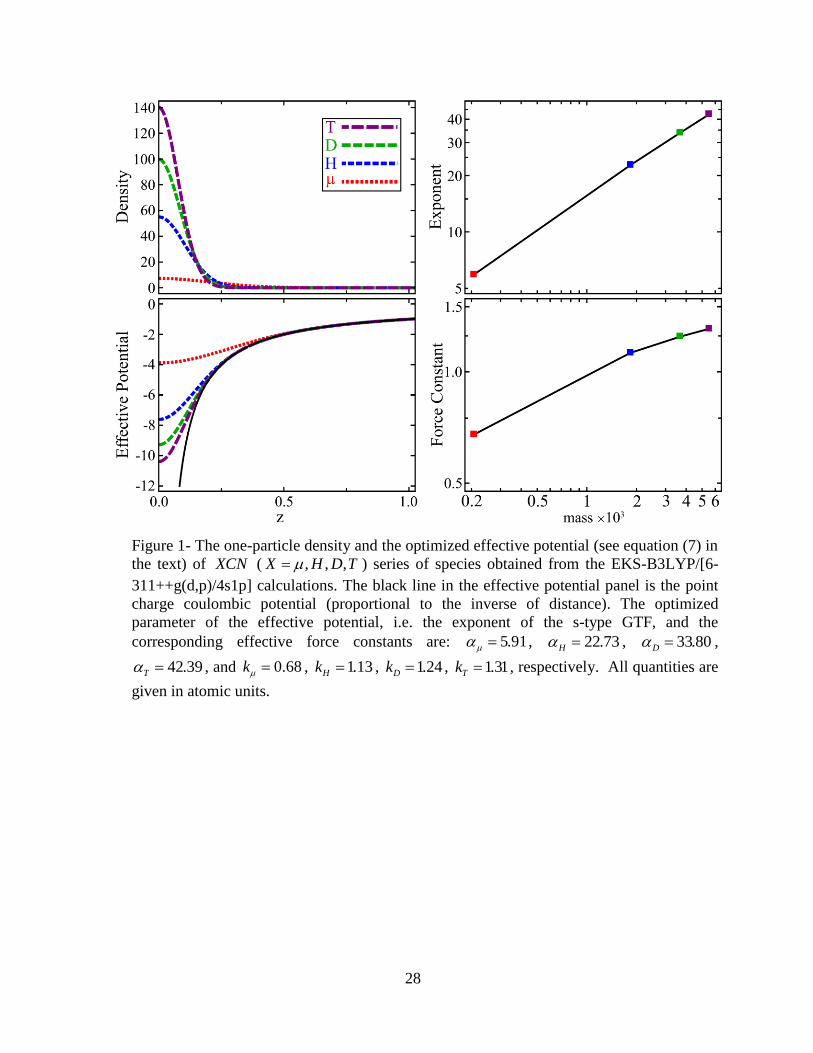
environment [39]. To have a clear picture of the mass-dependence of the effective
potential in the EKS equations a comparative study was done on XCN ( , , ,X H D T )
species, where the carbon and nitrogen nuclei were considered as clamped point charges
while X was treated as a quantum particle. Figure 1 offers the final optimized results of
the EKS calculations revealing that the effective potential associated to the heavier particle
has less deviations from the point charge coulombic potential far from the banquet center
while its one-particle density is more localized. These observations are in line with the
expectation that a massive quantum particle behaves more like a clamped point charge than
a lighter one. To have a quantified picture of these variations the effective potentials in
equations (5) and (7) are rewritten using the known mass-dependence of from the
isotropic harmonic oscillator model [94]:
41e
eff i i c
i c
v r erf km r Rr R
43, , ,
4
q
c c
c
ZkU k m R R erf km R R
m R R
(11)
In these potentials k stands for the force constant which is mainly characteristic of the
environment and theoretically, independent from the mass. Thus, the model is to be taken
seriously only when slight variation of this effective force constant is seen upon isotopic
substitution in the EKS calculations. To test the reliability of the model, Figure 1 compares
the mass-dependence of the optimized and k values demonstrating that the latter is

15
indeed much less sensitive to the mass variations, and may even be treated as a constant in
the case of the hydrogen isotopes. This observation reveals that equations (11) are reliable
for modeling the intrinsic mass-dependence of the effective potential while the smaller
variations of the potentials induced by the variations of the environment are all absorbed in
the effective force constant. If ab initio EKS calculations demonstrate that the variations of
the effective force constant in a certain set of muonic species are also small, then it is
legitimate to introduce a “mean” and corresponding mean effective potential for the
corresponding set. The introduction of the mean effective potentials particularly bypasses
the costly non-linear optimization of for each species separately.
Seven small organic molecules: diazene, acetylene, methenamine, hydrogen
cyanide, formamide, fomaldehyde, and ethylene, where their atom types and bonds are
typical to many organic molecules used in the experimental μSR studies [1,3], were
selected as the representative set. Since in the corresponding experiments muonium atom
( plus an electron) is attached to organic molecules, we have also attached muonium
atom to these seven molecules and the resulting set of open-shell muonic species was
employed in order to evaluate the numerical values of . Practically, to have an initial
geometry, a hydrogen atom with a clamped proton was first attached to the molecules of
the representative set and from various possible conformers the lower energy minima were
extracted after the geometry optimization at B3LYP/6-311++g(d,p) level. In next step, a
muonium atom replaced the hydrogen atom, i.e. a banquet atom and corresponding
electronic [4s1p] basis functions were added instead of hydrogen atom. Subsequently, the
position of the banquet atoms, and the exponents of [4s1p] electronic basis set were
simultionsly optimized while the geometry of the remaining nuclei was held fixed. The

16
resulting eleven low-energy muoniated structures are depicted in Figure 2 while the
corresponding final optimized geometries have been given in the supporting information.
Table 1 offers the optimized values at both EKS-UB3LYP/[6-311++g(d,p)/4s1p] and
EKS-ROB3LYP/[6-311++g(d,p)/4s1p] levels of calculations; the resulting optimized
values are distributed narrowly, 6.05 0.1EKS , and insensitive to the U or the RO
versions of the EKS calculations. This is not far from the mean derived from the EHF
calculations in the previous study on a completely different set of closed-shell muonic
species [39], 5.75EHF , and confirms that the idea of the mean effective potential is
reliable enough to be used in the EKS calculations. On the other hand, in the previous EHF
study the mean exponents of the basis functions in the extended muonic [2s2p2d] basis set
were narrowly distributed around the mean: 0.8 1.4EHF EHF [39]. In present study the
exponents of [5s5p] muonic basis set were also scaled around the mean:
0.5 , 0.75 , , 1.5 , 2.0EKS EKS EKS EKS EKS . Then, they are used in the construction of
corresponding extended effective potential, which in contrast to the simple effective
potentials in equations (5) and (7), includes the anharmonicity and the anisotropy of ’s
vibrations (for a thorough discussion see [39]). Hence, only the linear coefficients in the
extended effective potential were optimized during the EKS calculations (see the
supporting information of [39] for details of the procedure). The exponents of the
electronic [4s1p] basis set were also optimized both at EKS-UB3LYP/[6-
311++g(d,p)/4s1p] and EKS-ROB3LYP/[6-311++g(d,p)/4s1p] levels and the final results
have been gathered in Table 2. Once again, it is evident from this table that the optimized
exponents are relatively insensitive to chemical environment and the mean values are
proper representatives for the optimized exponents. Therefore, the mean values derived at

17
the EKS-UB3LYP/[6-311++g(d,p)/4s1p] level will be used in the rest of this paper. The
computed mean exponents are comparable to the mean exponents derived in the previous
study using the EHF equations: 4.21, 1.20, 0.37, 0.12, 0.58s p [39], and are
insensitive to the U and the RO versions of the EKS calculations as well.
B. Muoniated ferrocenyl radicals
The idea of adding muonium atoms to organic molecules is not new [1], by the way,
more recently muonium atoms have been attached also to carbenes, their organosilicon
analogs and organometallic molecules [95,96]. One of the interesting organometallic
targets considered both experimentally and computationally is the iconic ferrocene
molecule though the corresponding experimental μSR spectrum of its muoniated radical is
not yet conclusively assigned [97-99]. Taking the size of ferrocene molecule, all previous
computational studies employed DFT to model this system where instead of the muonium
atom, a hydrogen atom with a clamped nucleus has been added to ferrocene [97,99]. In this
section the EKS-UB3LYP/[6-311++g(d,p)/4s1p] method is used in conjunction with the
extended effective potential developed in the previous section in order to study the
muoniated ferrocenyl radicals.
In order to start the calculations, we reoptimized the ferrocenyl radical structures
reported by McKenzie at UB3LYP/6-311++g(d,p) level [99]. The four optimized
structures include ferrocenyl radicals after hydrogen addition to cyclopentadienyl ring or
the iron atom while considering the relative configuration of the cyclopentadienyl (Cp)
rings that could be staggered or eclipsed [99]. In the next step, the hydrogen atom was
eliminated from the structures and a banquet atom with a [4s1p] basis set was added
instead. In the case of radicals originating from adding hydrogen atom to the Cp ring,

18
banquet atom could be placed at exo, i.e. with the farthest distance to the iron center, or
endo, i.e. with the closest distance to the iron center, positions. Therefore, six distinct
muoniated structures were prepared and the EKS-UB3LYP/[6-311++g(d,p)/4s1p] method
along with the geometry optimization were applied. Figure 3 depicts the final optimized
structures and the used nomenclature while supporting information contains the optimized
coordinates. In the case of exo-Cp-eclipsed, endo-Cp-eclipsed and Fe-staggered structures,
the full geomtry optimization did not yield stable structures thus they were derived by
imposing a plane of symmetry as a contriant. Indeed, the hydorgenic analogs of these
structures are saddle points on the corresponding energy hypersurface as reproted by
McKenzie and independently confirmed in the present study [99]. Figure 3 also contains
the “mean “distance between and neighboring nucleus; it is important to stress that this
mean distance is distinct from the distance between banquet center and neighboring
nucleus and is the expectation value of ’s position operator where the neighboring
nucleus is at the center of the coordinate system. The mean C- distances, 1.16 - 1.18 Å,
if compared to usual C-H distances, 1.08 - 1.10 Å, are quite longer revealing the
nonnegligible elongations of the bond lengths upon isotopic substitution. This trend is
completely absent in the conventional ab initio calculations based on using a clamped
hydrogen atom to model muonium addition to molecular systems. This observation is in
line with one of our previous studies where substitution of with one of the hydrogen
atoms of malonaldehyde varied the conformation drastically [37]. All observed traits point
to the fact that even at the structural level the EKS results contain novel information that
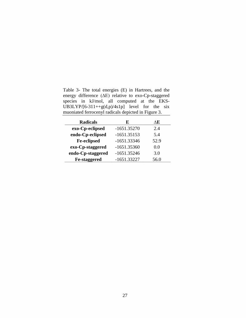
are absent if the clamped nucleus model be used instead. Table 3 includes the total and
relative energies for the considered species revealing that exo-Cp-staggered radical is the

19
most stable species in line with McKenzie’s results [99]. As stressed before, (exo/endo)-
Cp-ecllipesed radicals are not stable structures, and threfore, the next stable structure is the
exo-Cp-staggered radical, which is only ~3 kJ/mol less stable than the correspodning exo
radical whereas the Fe-ecplised radical is ~53 kJ/mol less table than the exo. Thus, it
seems reasonable to assume that only the Cp-staggered conformer has a major contribution
in the muoniation in gas phase though as disucssed in detail by McKenzie [99], in the solid-
state uncertainties emerge due to the crystal packing effects and possible structural
deformations of ferreocne molecule itself.
V. Conclusion
The present study demonstrates that the basic idea of the effective theory, proposed
recently [38,39], is extendable both theoretically and computationally to the DFT of
muonic systems. Nevertheless, this is just a primary result and it is desirable to include ee
correlation at the wavefunction-based levels of the effective theory as well as devising the
effective version of the NEO-DFT(ee+eµ), both will be discussed in subsequent reports. In
the meantime, the EKS equations provide a framework to start studying the structural and
energetic aspects of large muonic systems though without including eµ correlation the
quantitative prediction of the μSR spectrum remains yet elusive. The EKS equations may
also yield the required information, e.g. one-particle densities, for “atoms in molecules”
study of muonic species as considered in some previous reports [34-37]. This path is also
now under scrutiny in our laboratory and the results will be discussed in future
communications.
Conflicts of interest
There are no conflicts of interest to declare.

20
Acknowledgments
The authors are grateful to Cina Foroutan-Nejad for detailed reading of this paper.
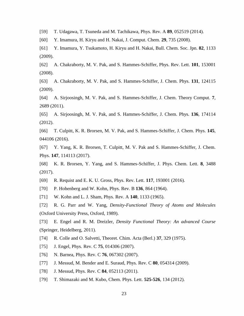
References
[1] E. Roduner, The Positive Muon as a Probe in Free Radical Chemistry (Lecture
Notes in Chemistry, Vol. 49, Springer, Berlin, 1988).
[2] S. J. Blundell, Contemp. Phys. 40, 175 (1999).
[3] K. Nagamine, Introductory Muon Science (Cambridge University Press,
Cambridge, 2003).
[4] S. J. Blundell, Chem. Rev. 104, 5717 (2004).
[5] J. H. Brewer, Phys. Proc. 30, 2 (2012).
[6] L. Nuccio, L. Schulz, and A. J. Drew, J. Phys. D: Appl. Phys. 47, 473001 (2014).
[7] J. Phys. Soc. Jap. 85, No. 9 (2016), Special Topics: Recent Progress of Muon
Science in Physics, 091001-091016.
[8] K. Wang, P. Murahari, K. Yokoyama, J. S. Lord, F. L. Pratt, J. He, L. Schulz, M.
Willis, J. E. Anthony, N. A. Morley, L. Nuccio, A. Misquitta, D. J. Dunstan, K.
Shimomura, I. Watanabe, S. Zhang, P. Heathcote and A. J. Drew, Nature Mat. 16, 467
(2017).
[9] C. G. Van de Walle, Phys. Rev. Lett. 64, 669 (1990).
[10] A. R. Porter, M. D. Towler, and R. J. Needs, Phys. Rev. B 60, 13534 (1999).
[11] D. Cammarere, R. H. Scheicher, N. Sahoo, T. P. Das, and K. Nagamine, Physica B
289-290, 636 (2000).
[12] C. P. Herrero and R. Ramírez, Phys. Rev. Lett. 99, 205504 (2007).
[13] H. Maeter, H. Luetkens, Yu. G. Pashkevich, A. Kwadrin, R. Khasanov, A. Amato,
A. A. Gusev, K. V. Lamonova, D. A. Chervinskii, R. Klingeler, C. Hess, G. Behr, B.
Büchner, and H.-H. Klauss, Phys. Rev. B 80, 094524 (2009).
[14] E. V. Sheely, L. W. Burggraf, P. E. Adamson, X. F. Duan, and M. W. Schmidt, J.
Phys.: Conf. Ser. 225, 012049 (2010).
[15] E. L. Silva, A. G. Marinopoulos, R. C. Vilão, R. B. L. Vieira, H. V. Alberto, J.
Piroto Duarte, and J. M. Gil, Phys. Rev. B 85, 165211 (2012).

21
[16] F. Bernardini, P. Bonfâ, S. Massidda, and R. De Renzi, Phys. Rev. B 87, 115148
(2013).
[17] P. Bonfà, F. Sartori and R. De Renzi, J. Phys. Chem. C 119, 4278 (2015).
[18] R. B. L. Vieira, R. C. Vilão, A. G. Marinopoulos, P. M. Gordo, J. A. Paixão, H. V.
Alberto, J. M. Gil, A. Weidinger, R. L. Lichti, B. Baker, P. W. Mengyan, and J. S. Lord,
Phys. Rev. B 94, 115207 (2016).
[19] S. J. Blundell, J. S. Möller, T. Lancaster, P. J. Baker, F. L. Pratt, G. Seber, and P.
M. Lahti, Phys. Rev. B 88, 064423 (2013).
[20] F. R. Foronda, F. Lang, J. S. Möller, T. Lancaster, A. T. Boothroyd, F. L. Pratt, S. R.
Giblin, D. Prabhakaran, and S. J. Blundell, Phys. Rev. Lett. 114, 017602 (2015).
[21] P. Bonfà and R. De Renzi, J. Phys. Soc. Jap. 85, 091014 (2016).
[22] R. M. Valladares, A. J. Fisher, and W. Hayes, Chem. Phys. Lett. 242, 1 (1995).
[23] M. I. J. Probert, and A. J. Fisher, Chem. Phys. Lett. 259, 271 (1996).
[24] M. I. J. Probert, and A. J. Fisher, J. Phys.: Condens. Matter 9, 3241 (1997).
[25] Y. K. Chen, D. G. Fleming, and Y. A. Wang, J. Phys. Chem. A 115, 2765 (2011).
[26] D. G. Fleming, D. J. Arseneau, M. D. Bridges, Y. K. Chen, and Y. A. Wang, J.
Phys. Chem. C 117, 16523 (2013).
[27] K. Yamada, Y. Kawashima, and M. Tachikawa, J. Chem. Theory Comput. 10, 2005
(2014).
[28] Y. Oba, T. Kawatsu, and M. Tachikawa, J. Chem. Phys. 145, 064301 (2016).
[29] A. Szabo and N. S. Ostlund, Modern Quantum Chemistry: Introduction to
Advanced Electronic Structure Theory (Dover Publications Inc., New York, 1996).
[30] T. Helgaker, P. Jørgenson, and J. Olsen, Molecular Electronic-Structure Theory
(John Wiley & Sons, New York, 2000).
[31] S. P. Webb, T. Iordanov, and S. Hammes-Schiffer, J. Chem. Phys. 117, 4106
(2002).
[32] T. Iordanov and S. Hammes-Schiffer, J. Chem. Phys. 118, 9489 (2003).
[33] C. Swalina, M. V. Pak, and S. Hammes-Schiffer, Chem. Phys. Lett. 404, 394
(2005).
[34] M. Goli and Sh. Shahbazian, Phys. Chem. Chem. Phys. 16, 6602 (2014).
[35] M. Goli and Sh. Shahbazian, Phys. Chem. Chem. Phys. 17, 245 (2015).

22
[36] M. Goli and Sh. Shahbazian, Phys. Chem. Chem. Phys. 17, 7023 (2015).
[37] M. Goli and Sh. Shahbazian, Chem. Eur. J. 22, 2525 (2016).
[38] M. Gharabaghi and Sh. Shahbazian, Phys. Lett. A 380, 3983 (2016).
[39] M. Ryaka, M. Goli, and Sh. Shahbazian, Phys. Chem. Chem. Phys. 20, 4466
(2018).
[40] B. Auer and S. Hammes-Schiffer, J. Chem. Phys. 132, 084110 (2010).
[41] L. M. Sander, H. B. Shore and L. J. Sham, Phys. Rev. Lett. 31, 533 (1973).
[42] R. K. Kalia and P. Vashishta, Phys. Rev. B 17, 2655 (1978).
[43] R. M. Nieminen, E. Boroński and L. J. Lantto, Phys. Rev. B 32, 1377 (1985).
[44] J. F. Capitani, R. F. Nalewajski and R. G. Parr, J. Chem. Phys. 76, 568 (1983).
[45] H. Englisch and R. Englisch, Phys. Stat. Sol. 123, 711 (1984).
[46] E. S. Kryachko, E. V. Ludeńa and V. Mujica, Int. J. Quantum Chem. 40, 589
(1991).
[47] N. Gidopoulos, Phys. Rev. B 57, 2146 (1998).
[48] T. Kreibich and E. K. U. Gross, Phys. Rev. Lett. 86, 2984 (2001).
[49] T. Kreibich, R. van Leeuwen and E. K. U. Gross, Phys. Rev. A 78, 022501 (2008).
[50] M. Tachikawa, K. Mori, H. Nakai and K. Iguchi, Chem. Phys. Lett. 290, 437
(1998).
[51] H. Nakai, Int. J. Quantum Chem. 107, 2849 (2007).
[52] T. Ishimoto, M. Tachikawa and U. Nagashima, Int. J. Quantum Chem. 109, 2677
(2009).
[53] R. Flores-Moreno, E. Posada, F. Moncada, J. Romero, J. Charry, M. Díaz-Tinoco,
S. A. González, N. F. Aguirre and A. Reyes, Int. J. Quantum Chem. 114, 50 (2014).
[54] Y. Shigeta, H. Takahashi, S. Yamanaka, M. Mitani, H. Nagao and K. Yamaguchi,
Int. J. Quantum Chem. 70, 659 (1998).
[55] T. Udagawa and M. Tachikawa, J. Chem. Phys. 125, 244105 (2006).
[56] M. V. Pak, A. Chakraborty, and S. Hammes-Schiffer, J. Phys. Chem. A 111, 4522
(2007).
[57] Y. Kita and M. Tachikawa, Comput. Theor. Chem. 975, 9 (2011).
[58] Y. Kita, H. Kamikubo, M. Kataoka and M. Tachikawa, Chem. Phys. 419, 50
(2013).
23
[59] T. Udagawa, T. Tsuneda and M. Tachikawa, Phys. Rev. A 89, 052519 (2014).
[60] Y. Imamura, H. Kiryu and H. Nakai, J. Comput. Chem. 29, 735 (2008).
[61] Y. Imamura, Y. Tsukamoto, H. Kiryu and H. Nakai, Bull. Chem. Soc. Jpn. 82, 1133
(2009).
[62] A. Chakraborty, M. V. Pak, and S. Hammes-Schiffer, Phys. Rev. Lett. 101, 153001
(2008).
[63] A. Chakraborty, M. V. Pak, and S. Hammes-Schiffer, J. Chem. Phys. 131, 124115
(2009).
[64] A. Sirjoosingh, M. V. Pak, and S. Hammes-Schiffer, J. Chem. Theory Comput. 7,
2689 (2011).
[65] A. Sirjoosingh, M. V. Pak, and S. Hammes-Schiffer, J. Chem. Phys. 136, 174114
(2012).
[66] T. Culpitt, K. R. Brorsen, M. V. Pak, and S. Hammes-Schiffer, J. Chem. Phys. 145,
044106 (2016).
[67] Y. Yang, K. R. Brorsen, T. Culpitt, M. V. Pak and S. Hammes-Schiffer, J. Chem.
Phys. 147, 114113 (2017).
[68] K. R. Brorsen, Y. Yang, and S. Hammes-Schiffer, J. Phys. Chem. Lett. 8, 3488
(2017).
[69] R. Requist and E. K. U. Gross, Phys. Rev. Lett. 117, 193001 (2016).
[70] P. Hohenberg and W. Kohn, Phys. Rev. B 136, 864 (1964).
[71] W. Kohn and L. J. Sham, Phys. Rev. A 140, 1133 (1965).
[72] R. G. Parr and W. Yang, Density-Functional Theory of Atoms and Molecules
(Oxford University Press, Oxford, 1989).
[73] E. Engel and R. M. Dreizler, Density Functional Theory: An advanced Course
(Springer, Heidelberg, 2011).
[74] R. Colle and O. Salvetti, Theoret. Chim. Acta (Berl.) 37, 329 (1975).
[75] J. Engel, Phys. Rev. C 75, 014306 (2007).
[76] N. Barnea, Phys. Rev. C 76, 067302 (2007).
[77] J. Messud, M. Bender and E. Suraud, Phys. Rev. C 80, 054314 (2009).
[78] J. Messud, Phys. Rev. C 84, 052113 (2011).
[79] T. Shimazaki and M. Kubo, Chem. Phys. Lett. 525-526, 134 (2012).

24
[80] P. M. W. Gill and R. D. Adamson, Chem. Phys. Lett. 261, 105 (1996).
[81] A. D. Becke, J. Chem. Phys. 88, 2547 (1988).
[82] A. D. Becke, J. Chem. Phys. 89, 2993 (1988).
[83] C. W. Murray, N. C. Handy, and G. J. Laming, Mol. Phys. 78, 997 (1993).
[84] O. Treutler and R. Ahlrichs, J. Chem. Phys. 102, 346 (1995).
[85] K. Capelle and V. L. Campo, jr., Phys. Rep. 528, 91 (2013).
[86] W. J. Hehre, R. Ditchfield, and J. A. Pople, J. Chem. Phys. 56, 2257 (1972).
[87] P. C. Hariharan and J. A. Pople, Theoret. Chim. Acta 28, 213 (1973).
[88] T. Clark, J. Chandrasekhar, G.W. Spitznagel, and P. v. R. Schleyer. J. Comp. Chem.
4, 294 (1983).
[89] A. D. Becke, Phys. Rev. A 38, 3098 (1988).
[90] C. Lee, W. Yang, and R. G. Parr, Phys. Rev. B 37, 785 (1988).
[91] A. D. Becke, J. Chem. Phys. 98, 5648 (1993).
[92] M. W. Schmidt, K. K. Baldridge, J. A. Boatz, S. T. Elbert, M. S. Gordon, J. H.
Jensen, S. Koseki, N. Matsunaga, K. A. Nguyen, S. Su, T. L. Windus, M. Dupuis and J. A.
Montgomery, J. Comput. Chem. 14, 1347 (1993).
[93] M. S. Gordon and M. W. Schmidt, Theory and Applications of Computational
Chemistry: the first forty years, pp. 1167-1189, Eds. C. E. Dykstra, G. Frenking, K. S. Kim,
G. E. Scuseria (Elsevier, Amsterdam, 2005).
[94] M. Goli and Sh. Shahbazian, Theor. Chem. Acc. 132, 1362 (2013).
[95] R. West and P. W. Percival, Dalton Trans. 39, 9209 (2010).
[96] R. West, K. Samedov and P. W. Percival, Chem. Eur. J. 20, 9184-9190 (2014).
[97] R. M. Macrae, Physica B 374-375, 307 (2006).
[98] U. A. Jayasooriya, R. Grinter, P. L. Hubbard, G. M. Aston, J. A. Stride, G. A.
Hopkins, L. Camus, I. D. Reid, S. P. Cottrell and S. F. J. Cox, Chem. Eur. J. 13, 2266
(2007).
[99] I. McKenzie, Phys. Chem. Chem. Phys. 16, 10600 (2014).

25
Tables:
Table 1- The optimized values (in atomic
units) derived at EKS-UB3LYP/[6-
311++g(d,p)/4s1p] and EKS-ROB3LYP/[6-
311++g(d,p)/4s1p] levels for the eleven
representative set of the muoniated species
depicted in Figure 2.
backbone U RO
Acetylene 6.10 6.10
Diazene 6.10 6.10
Ethylene 6.16 6.16
C-Formaldehyde 5.98 5.99
O-Formaldehyde 5.98 5.98
C-Formamide 6.07 6.07
O-Formamide 5.91 5.91
C-Hydrogen cyanide 6.02 6.03
N-Hydrogen cyanide 5.95 5.95
C-Methenamine 6.15 6.16
N-Methenamine 6.14 6.15
mean 6.05 6.05

26
Table 2- The optimized exponents (in atomic units) of [4s1p] electronic basis
set derived at EKS-UB3LYP/[6-311++g(d,p)/4s1p] and EKS-ROB3LYP/[6-
311++g(d,p)/4s1p] levels for the eleven representative set of the muoniated
species depicted in Figure 2.
U S S S S P
Acetylene 3.90 1.02 0.35 0.13 0.81
Diazene 3.87 0.98 0.31 0.09 0.79
Ethylene 3.89 0.99 0.31 0.11 0.87
C-Formaldehyde 3.76 0.96 0.29 0.09 0.80
O-Formaldehyde 4.31 1.17 0.38 0.11 0.68
C-Formamide 3.85 0.97 0.30 0.09 0.97
O-Formamide 4.24 1.17 0.39 0.12 0.71
C-Hydrogen cyanide 3.51 0.86 0.27 0.08 0.88
N-Hydrogen cyanide 3.91 1.02 0.33 0.09 0.70
C-Methenamine 3.75 0.94 0.29 0.09 0.88
N-Methenamine 4.19 1.09 0.36 0.10 0.77
mean 3.92 1.01 0.33 0.10 0.81
RO S S S S P
Acetylene 3.72 0.94 0.31 0.11 0.82
Diazene 3.78 0.96 0.31 0.08 0.79
Ethylene 3.73 0.94 0.29 0.09 0.88
C-Formaldehyde 3.70 0.94 0.29 0.09 0.81
O-Formaldehyde 4.34 1.18 0.39 0.11 0.68
C-Formamide 3.77 0.95 0.30 0.09 0.96
O-Formamide 4.30 1.18 0.39 0.12 0.71
C-Hydrogen cyanide 3.43 0.84 0.26 0.07 0.88
N-Hydrogen cyanide 3.86 1.00 0.33 0.09 0.70
C-Methenamine 3.67 0.92 0.28 0.08 0.88
N-Methenamine 4.10 1.07 0.35 0.10 0.77
mean 3.85 0.99 0.32 0.09 0.81
27
Table 3- The total energies (E) in Hartrees, and the
energy difference (∆E) relative to exo-Cp-staggered
species in kJ/mol, all computed at the EKS-
UB3LYP/[6-311++g(d,p)/4s1p] level for the six
muoniated ferrocenyl radicals depicted in Figure 3.
Radicals E ∆E
exo-Cp-eclipsed -1651.35270 2.4
endo-Cp-eclipsed -1651.35153 5.4
Fe-eclipsed -1651.33346 52.9
exo-Cp-staggered -1651.35360 0.0
endo-Cp-staggered -1651.35246 3.0
Fe-staggered -1651.33227 56.0
28
Figure 1- The one-particle density and the optimized effective potential (see equation (7) in
the text) of XCN ( , , ,X H D T ) series of species obtained from the EKS-B3LYP/[6-
311++g(d,p)/4s1p] calculations. The black line in the effective potential panel is the point
charge coulombic potential (proportional to the inverse of distance). The optimized
parameter of the effective potential, i.e. the exponent of the s-type GTF, and the
corresponding effective force constants are: 5.91 , 22.73H , 33.80D ,
42.39T , and 0.68k , 1.13Hk , 1.24Dk , 1.31Tk , respectively. All quantities are
given in atomic units.

29
Figure 2- The structures of muoniated (a) diazene, (b) acetylene, (c) N-methenamine, (d)
C-methenamine, (e) N-hydrogen cyanide, (f) C-hydrogen cyanide, (g) O-formamide, (h) C-
formamide, (i) O-fomaldehyde, (j) C-fomaldehyde, and (k) ethylene adducts (N, C and O
symbols are used to descriminate muon’s attachment site). Blue, grey, red, white and green
spheres indicate the locations of nitrogen, carbon, oxygen, hydrogen and muonium banquet
atoms, respectively.

30
Figure 3- The equilibriumm structures of ferrocene muoniated adducts (a) exo-Cp-eclipsed,
(b) endo-Cp-eclipsed, (c) Fe-eclipsed, (d) exo-Cp-staggered, (e) endo-Cp-staggered and (f)
Fe-staggered. The mean inter-nuclear distance between muonium (banquet) atom and its
binding site (neigboring nucleus) for each adduct has been given over the corresponding
bond (in angstroms). Orange, grey, white and green spheres indicate the locations of iron,
carbon, hydrogen and muonium (banquet) atoms, respectively.

1
Supporting Information
Effective electronic-only Kohn-Sham equations for the muonic
molecules
Milad Rayka1, Mohammad Goli2,* and Shant Shahbazian1,*
1 Department of Physics and Department of Physical and Computational
Chemistry, Shahid Beheshti University, G. C., Evin, Tehran, Iran, 19839, P.O. Box
19395-4716.
2 School of Nano Science, Institute for Research in Fundamental Sciences (IPM),
Tehran 19395-5531, Iran
E-mails:
Mohammad Goli : [email protected]
Shant Shahbazian: [email protected]
* Corresponding authors

2
Table of contents
Pages 3 - 8: The Cartesian coordinates of the optimized muoniated structures depicted in Figure
2 in the main text.
Pages 9 - 14: The Cartesian coordinates of the optimized muoniated ferrocenyl radicals depicted
in Figure 3 in the main text.

3
Mu-acetylene
Atom
type
Nuclear
charge
Coordinates (Angstrom)
X Y Z
C 6 0.04801 -0.58616 0.00000
Mu 1 -0.94683 -1.20419 0.00000
H 1 0.96878 -1.16584 0.00000
C 6 0.04801 0.71926 0.00000
H 1 -0.66429 1.53126 0.00000
Mu-diazene
Atom
type
Nuclear
charge
Coordinates (Angstrom)
X Y Z
N 7 0.74076 -0.15096 0.02319
H 1 1.15164 0.78554 -0.03051
N 7 -0.59555 0.02444 -0.06746
H 1 -1.13599 -0.80167 0.14495
Mu 1 -1.07993 0.96698 0.17820

4
Mu-ethylene
Atom
type
Nuclear
charge
Coordinates (Angstrom)
X Y Z
C 6 -0.69369 0.00000 -0.00200
H 1 -1.10645 -0.88654 -0.49274
H 1 -1.10645 0.88653 -0.49274
Mu 1 -1.12735 0.00000 1.09631
C 6 0.79390 0.00000 -0.01808
H 1 1.35196 0.92631 0.03997
H 1 1.35196 -0.92631 0.03997
Mu-C-formaldehyde
Atom
type
Nuclear
charge
Coordinates (Angstrom)
X Y Z
O 8 -0.79134 0.00000 0.00732
C 6 0.57435 0.00000 0.01424
H 1 1.00646 0.91035 0.45537
H 1 1.00646 -0.91034 0.45537
Mu 1 0.89218 0.00000 -1.13575

5
Mu-O-formaldehyde
Atom
type
Nuclear
charge
Coordinates (Angstrom)
X Y Z
C 6 -0.68511 -0.02779 0.05962
H 1 -1.11960 -0.99600 -0.15903
H 1 -1.23591 0.88841 -0.09062
O 8 0.67048 0.12557 -0.02145
Mu 1 1.15299 -0.78134 0.08705
Mu-C-formamide
Atom
type
Nuclear
charge
Coordinates (Angstrom)
X Y Z
N 7 1.19216 -0.10187 0.00000
H 1 1.35101 -0.67568 0.82140
H 1 1.35101 -0.67567 -0.82141
O 8 -1.21663 -0.37191 0.00000
C 6 -0.13539 0.46225 0.00000
Mu 1 -0.27518 1.18353 -0.93586
H 1 -0.25088 1.13307 0.87248
6
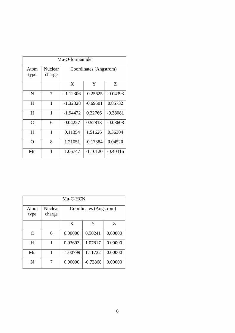
Mu-O-formamide
Atom
type
Nuclear
charge
Coordinates (Angstrom)
X Y Z
N 7 -1.12306 -0.25625 -0.04393
H 1 -1.32328 -0.69501 0.85732
H 1 -1.94472 0.22766 -0.38081
C 6 0.04227 0.52813 -0.08608
H 1 0.11354 1.51626 0.36304
O 8 1.21051 -0.17384 0.04520
Mu 1 1.06747 -1.10120 -0.40316
Mu-C-HCN
Atom
type
Nuclear
charge
Coordinates (Angstrom)
X Y Z
C 6 0.00000 0.50241 0.00000
H 1 0.93693 1.07817 0.00000
Mu 1 -1.00799 1.11732 0.00000
N 7 0.00000 -0.73868 0.00000

7
Mu-N-HCN
Atom
type
Nuclear
charge
Coordinates (Angstrom)
X Y Z
C 6 -0.00030 0.64744 0.00000
H 1 0.89589 1.28025 0.00000
N 7 -0.00030 -0.58320 0.00000
Mu 1 -0.95653 -1.12482 0.00000
Mu-C-methenamine
Atom
type
Nuclear
charge
Coordinates (Angstrom)
X Y Z
N 7 -0.80316 -0.15310 0.00000
H 1 -1.21222 0.78947 0.00000
C 6 0.62833 0.01211 0.00000
H 1 1.12743 -0.95854 0.00000
H 1 0.96848 0.58405 -0.87858
Mu 1 1.00018 0.61822 0.94259

8
Mu-N-methenamine
Atom
type
Nuclear
charge
Coordinates (Angstrom)
X Y Z
C 6 -0.72897 0.00000 0.07812
H 1 -1.24362 -0.93097 -0.11838
H 1 -1.24363 0.93097 -0.11839
N 7 0.65504 0.00000 -0.09205
H 1 1.13790 0.83602 0.20621
Mu 1 1.17885 -0.89694 0.20848

9
exo-Cp-staggered
Atom Charge Coordinates (Angstrom)
X Y Z
C 6 4.58331 1.34874 0.00087
C 6 4.28455 0.57184 -1.14566
C 6 4.28319 0.56404 1.14185
C 6 3.86885 -0.72852 -0.71811
C 6 3.86834 -0.73332 0.70525
H 1 4.90815 2.37867 0.00460
H 1 4.37397 0.89710 -2.17191
H 1 4.37095 0.88270 2.17031
H 1 3.62205 -1.55676 -1.36540
H 1 3.62040 -1.56562 1.34689
Fe 26 2.43015 0.64833 -0.00339
C 6 1.09284 2.00836 -0.72137
C 6 1.09351 2.01294 0.70742
C 6 0.71950 0.70493 -1.14651
C 6 0.72062 0.71223 1.14128
C 6 0.00000 0.00000 0.00000
H 1 1.39915 2.82811 -1.35629
H 1 1.40042 2.83661 1.33696
H 1 0.62301 0.41484 -2.18441
H 1 0.62498 0.42872 2.18108
Mu 1 -1.11732 0.16641 -0.00004
H 1 0.15567 -1.08243 0.00327

10
endo-Cp-staggered
Atom Charge Coordinates (Angstrom)
X Y Z
C 6 4.58959 1.34689 -0.00093
C 6 4.28926 0.56055 -1.14067
C 6 4.29194 0.57174 1.14694
C 6 3.87466 -0.73605 -0.70195
C 6 3.87574 -0.72916 0.72149
H 1 4.91411 2.37691 -0.00633
H 1 4.37660 0.87777 -2.16960
H 1 4.38222 0.89845 2.17265
H 1 3.62743 -1.56946 -1.34247
H 1 3.63051 -1.55672 1.37025
Fe 26 2.43573 0.64653 0.00546
C 6 1.10122 2.01238 -0.70383
C 6 1.09970 2.00581 0.72470
C 6 0.72695 0.71206 -1.13968
C 6 0.72446 0.70162 1.14773
C 6 0.00000 0.00000 0.00000
H 1 1.41047 2.83640 -1.33192
H 1 1.40765 2.82386 1.36116
H 1 0.63355 0.43088 -2.18035
H 1 0.62905 0.41062 2.18552
H 1 -1.09212 0.17558 -0.00036
Mu 1 0.14839 -1.09955 -0.00487

11
exo-Cp-eclipsed
Atom Charge Coordinates (Angstrom)
X Y Z
C 6 4.54825 -0.70758 -0.50978
C 6 4.54736 0.70860 -0.50968
C 6 3.99679 -1.14808 0.73334
C 6 3.99536 1.14831 0.73347
C 6 3.68567 -0.00011 1.50973
H 1 4.89490 -1.34612 -1.30860
H 1 4.89328 1.34772 -1.30835
H 1 3.86371 -2.17556 1.03752
H 1 3.86113 2.17549 1.03806
H 1 3.25212 -0.00020 2.49933
Fe 26 2.48866 -0.00043 -0.28915
C 6 1.37178 -0.71599 -1.83149
C 6 1.37217 0.71435 -1.83182
C 6 0.80926 -1.14610 -0.60075
C 6 0.81001 1.14541 -0.60117
C 6 0.00000 0.00000 0.00000
H 1 1.79325 -1.34773 -2.60084
H 1 1.79403 1.34533 -2.60157
H 1 0.66954 -2.18453 -0.33126
H 1 0.67083 2.18412 -0.33246
Mu 1 -1.08406 0.00044 -0.31808
H 1 0.00219 -0.00020 1.09405

12
endo-Cp-eclipsed
Atom Charge Coordinates (Angstrom)
X Y Z
C 6 4.55382 -0.70764 -0.50563
C 6 4.55468 0.70865 -0.50594
C 6 4.00353 -1.14713 0.73820
C 6 4.00478 1.14926 0.73777
C 6 3.69465 0.00128 1.51457
H 1 4.89870 -1.34701 -1.30454
H 1 4.90035 1.34704 -1.30529
H 1 3.86964 -2.17414 1.04350
H 1 3.87219 2.17686 1.04183
H 1 3.26296 0.00067 2.50501
Fe 26 2.49499 0.00159 -0.28506
C 6 1.38124 -0.71424 -1.82773
C 6 1.38021 0.71588 -1.82791
C 6 0.81626 -1.14493 -0.59762
C 6 0.81450 1.14602 -0.59798
C 6 0.00000 0.00000 0.00000
H 1 1.80631 -1.34529 -2.59572
H 1 1.80399 1.34777 -2.59596
H 1 0.67950 -2.18398 -0.32889
H 1 0.67555 2.18486 -0.32948
H 1 -1.05768 -0.00098 -0.32393
Mu 1 -0.00786 0.00067 1.11038

13
Fe-eclipsed
ATOM ATOMIC Coordintes (Angstrom)
X Y Z
C 6 0.70005 1.65236 1.34099
C 6 -0.70591 1.65216 1.33737
C 6 0.70579 -1.65227 1.33742
C 6 -0.70015 -1.65240 1.34104
C 6 1.15075 1.83060 -0.00339
C 6 -1.14985 1.83073 -0.00920
C 6 1.14971 -1.83085 -0.00917
C 6 -1.15088 -1.83046 -0.00334
C 6 0.00259 2.01276 -0.82814
C 6 -0.00275 -2.01271 -0.82811
H 1 1.33558 1.49178 2.19883
H 1 -1.34558 1.49151 2.19213
H 1 1.34546 -1.49170 2.19219
H 1 -1.33566 -1.49169 2.19887
H 1 -2.17620 1.89495 -0.33733
H 1 2.17867 1.89477 -0.32663
H 1 -2.17880 -1.89438 -0.32660
H 1 2.17607 -1.89527 -0.33728
H 1 0.00522 2.25816 -1.87873
H 1 -0.00537 -2.25805 -1.87871
Fe 26 0.00000 0.00000 0.00000
Mu 1 0.00002 0.00002 -1.52429

14
Fe-staggered
Atom Charge Coordinates (Angstrom)
X Y Z
C 6 -1.64609 0.71573 -1.18184
C 6 -0.45784 1.14392 -1.83465
C 6 0.24921 0.00078 -2.28317
C 6 -0.45613 -1.14352 -1.83543
C 6 -1.64489 -0.71775 -1.18208
H 1 -2.42255 1.35442 -0.79080
H 1 -0.15841 2.17187 -1.97759
H 1 1.20444 0.00104 -2.78565
H 1 -0.15491 -2.17089 -1.97872
H 1 -2.42050 -1.35782 -0.79166
Fe 26 0.00000 0.00000 0.00000
C 6 0.65487 0.00016 2.07423
C 6 1.17236 1.15047 1.41057
C 6 2.09538 0.70096 0.41616
C 6 2.09430 -0.70344 0.41629
C 6 1.17068 -1.15121 1.41094
H 1 0.00497 0.00104 2.93531
H 1 0.96449 2.17784 1.66811
H 1 2.64835 1.33730 -0.25853
H 1 2.64628 -1.34093 -0.25811
H 1 0.96103 -2.17815 1.66877
Mu 1 -1.15470 0.00104 0.98778