effective federal individual income tax functions - national tax journal

EFFECTIVE FEDERAL INDIVIDUAL INCOME TAX FUNCTIONS: AN EXPLORATORY EMPIRICAL ANALYSIS MIGUEL GOUVEIA* & ROBERT P. STRAUSS**

Abstract - We define and statistically estimate a nonlinear relationship between individual effective income tax rates and economic income for United States tax return data for tax years 1979-89. The relationship, which we call the effective tax function, has three parameters and was theoretically derived from the theory of equal sacrifice by Young (1988, 1990) and more generally by Berliant and Gouveia (1993). Annual graphs of the statistically estimated effective tax functions are presented and used to characterize empirically the evolution of the United States federal tax system with respect to four characteristics of the tax system: average marginal tax rates, redistributional elasticities, revenue elasticities, and horizontal equity. For each characteristic, we present a preliminary assessment of the impact of the 1986 tax reform. The major empirical finding is that the effective income tax function exhibits a trend toward less progressivity for the years studied. This gen-

*Department of Economics, University of PennsylvanIa, 3718 Locust Walk, Philadelphia, PA 19104 **Department of Economics, University of Rochester, Roches- ter, NY 14627 and the Heinz School, Carnegie-Mellon Uni- versity, Pittsburgh, PA 152 13

eral conclusion is also valid for indexes that measure the redistributive impact of the tax system (the elasticity of after-tax income with respect to before-tax income) and the revenue effects of the system (the elasticity of fiscal revenue with respect to before-tax income).

I, . . a tax law is a mapping from a vector whose elements are the income characteristics of the individual (wage income, dividends, capital gains, and all the other items in the income tax form) to tax liabilities. It is supposed to be a well defined function; no economic analysis is needed. (. . .) In fact, to use this information one wants to know the distribution of the burden by some classification of lower dimen- sionality than that used in the tax law.” in Arrow (1980, p. 265).

INTRODUCTION

Few domestic fiscal issues can be as controversial as the income tax. The de- bates between successive Administra- tions and Congress over the tax rate structure of the federal individual in-

317

come tax and the treatment of capital gains illustrate the difficulty any demo- cratic society has iri reaching and main- taining a consensus on income taxation. Political difficulties notwithstanding, summarizing the effects of changes in income tax iaw from ex post data on taxes and income is far frorn a transparent matter to the research community.

It should be noted that the relationship between taxes and income contained in the tax law, what we call the statutory %ax function, can only be seen as an initial benchmark for the empirical relationship between taxes actually paid and economic income. We shall call this latter relationship the effective tax function.

A variety of researc:h strategies are available to characterize empirically over time ithe relationship between taxes paid and economic income to capture the effects of different tax law regimes. One approach has been to utilize an index number measure of the pre- and post- ltax distributions of income using, say, ithe Gini coefficient of lncorne inequality, and to compare thle calculated values across time.’

One can examine hypothetical, i.e., ex ante changes in liabilities, at a moment in time, by recalculating taxes due and summarizing the differences between ac- tual liabilities and hypothetical or simu- lated liabilities.* This methodology is routinely used by government agencies and Iuses complex microsimulation models that typically account for only a few be- Ihavioral taxpayer respor1ses.3 The differ- lential analyses usually performed through such models use the statutory Imarginal tax rates irather than the effective marginal tax rates to quantify reve- inue or burden distiribution changes. Al- though these models may be suitable for the differential analysis required to as- :jess changes in policy by focusing on

the effects of perturbations on the “status quo,” they do not provide a total “picture” of the tax system across time. Another approach is to Ilook directly each year at average tax payments by economic income strata, or at shares of taxes paid each year by income deciles.

Most recently, Young (1988, 1990) and Berliant and Gouveia (1993) have theoretically derived specific functional rela- tions between taxes and income that are consistent with legislators implicitly fa- voring tax systems based on the theory of equal sacrifice. Under this approach, one compares the parameters of the function across time.

It shoutd be noted that the statutory and effective tax functions differ for two reasons. First, taxable income varies markedly from economic income under most Income tax laws; typically eco- nomilc income is reduced substantially by a large number of exclu~sions, deductions, and the provision of personal exemptions Further, gross taxes due differ from net taxes by various credits. Sec- ond, to the extent that ‘taxpayers alter their behavior in response to the differential treatment of certain sources of income and/or the provision of ‘tax cred- Its, there is reason to expect that the effective tax function, an ex post concept, will differ from the statutory tax function.

With a statistically estimated effective tax function, which relates effective tax rates to economic income, we can readily examine and test statistically for changes in the shape of the relationship between taxes and economic income over time. OIur purpose #below is to im- plement empirically, and thereby demon- strate the utlility of, the statistical estimation of such a specific functional form for successive c:ross sectlions of United States data for a particularly tumultuous

318

I EFFECTIVE FEDERAL INDIVIDUAL TAX FUNCTIONS

period in American tax history, 1979- 89.4

Statistically estimated effective tax functions for each year allow us to display graphically the changing nature of the federal personal income tax for the period 1979-89. Further, the estimated effective tax functions in hand allow us to answer readily a number of important questions about the United States individual income tax during this period:

(1)

(2)

(3)

(4)

Have its disincentives on economic activity increased/decreased over time? How much does it contribute to income redistribution over time? How has its fiscal revenue produc- tivity been changing? Has the overall pattern of effective tax rates become more/less widely dispersed over time, perhaps indicative of changes in horizontal equity?

We shall answer the first question by computing the average marginal tax rate. This statistic can be considered a measure of the marginal distortion intro- duced by the income tax system in a representative taxpayer’s behavior. The Statistics of Income (501) data that we employ allow us to compute directly the average marginal statutory tax rate. By using our estimates of the effective income tax function, we are also able to present estimates of the average marginal effective tax rates.

These effective averages are lower than the statutory averages, and they exhibit a downward trend from 1980 to 1986, reversed in 1987.5 Interestingly, this reversal occurs despite the fall in statutory marginal tax rates. This could be interpreted as a sign that the tax reform of 1986 was successful in eliminating some tax incentives/loopholes and was successful in broadening the income tax base. Alternatively, 1987 may be an anomaly due to capital gains adjust-

ments made by the taxpayers in 1986. However, the effects of the reform seem to have been short-lived: the results for 1988 and 1989 show a return to pre- reform levels.

The second and third questions are both related to the progressivity of the income tax. While direct measures of progressivity are not presented, we concen- trate here on the implications of progressivity for income inequality reduction and revenue responsiveness to income changes.

The second statistic is the mean elasticity6 of after-tax income with respect to before-tax or gross income. The information provided by this elasticity can be best seen as follows: if one starts with a given before-tax income distribution, the after-tax income distribution will be less “unequal” the smaller the elasticity. A proportional tax system has a unitary elasticity and a progressive tax system has an elasticity below one. The empirical results show that this elasticity is less than one, but also that it increased from 1980 to 1989, with an exception in 1987.

The third statistic we compute is the income elasticity of the revenue raised by the individual income tax. This elasticity gives the percentage increase in revenue when all individual incomes increase by one percent and has often been described as the built-in flexibility of the income tax. The empirical results show that this elasticity has been decreasing since 1979, although not in a monotonic way.

When looking at the three statistics mentioned above, one should keep in mind that they result not only from the properties of the effective tax functions but also from the characteristics of the contemporaneous income distributions. With the knowledge of the effective tax functions, it becomes possible to sepa-

319

rate the roles of the individual income tax system on one side, and of the income distribution on the other, in gen- erating the aggregate statistics we often encounter bn public policy discussions. In particular, we can easily perform (static) counterfactual analysis: had the effective tax function stayed the same, how would results change with a different distribution of Income? This should be seen not as a forecasting exercise (for which we would need also to account for behavior changes) but instead as an alternative way to characterize the tax structure.

Finally, our answer to the dispersion or horizontat equity question is based on the mean squared error (MSE) of the estimated tax iunctions. Despite several limitations that we will discuss later, we suggest that the MSE can help measure the horizontal inequity of the income tax system. We find that the horizontal equity characteristics of the federal individual income tax have been fluctuating during the period covered by our study. The immediate impact of the 1986 reform was a reduction in horizontal inequity. However, the situation worsened after 1987.

We should also note that the use of a statistically estimated effective tax function has several aclvantages over the traditional method of computing average taxes for given intervals of the income distribution (e.g., deciles). In particular, using the regression estimates, we can compute average itaxes for any income level, and it IS easy to do statistical inference and testing. We also have a simple way to estimate marginal taxes and elasticities. Additionally, a statistically estimated nonlinear effective tax function is better able to hanIdle the nonlinearities in the data This becomes important when the income intervals are large, as is typically i:he case with the top quintile or deci)e.7

The organization of the paper is a follows. Section 2 discusses the measures of income and taxes to be used in the estimation of the effective tax functions. Sectnon 3 presents the functional form used for the effective tax function and the results of its nonliniear statistical estimation. In Section 4, ve apply the estimated effective tax functions to generate estimates of effective average tax functions, redistributional effects, an index of horizontal inequity, and the calculation of revenue elasticities. Section 5 concludes with suggestions for future research.

THE MEASURES OF INCOME AND TAXES

This section discusses the data empirically investigated below and discusses the operational definitibns of the main concepts used in the p8per. To estimate the effective individual income tax functions, we use individual income and tax data routinely made avgilable in anonymous, public use samples of tax returns by the SOI division of the Internal Reve- nue Service.8 These samples contain tax return data for large (a~bout 100,000 per year) cross sections of taxpayers.

We take the tax return as the unit of analysis and include in our income definition all sourc:es of income identifiable frorr tax returns: labor income, interest, dividends, capital gains (“grossed up” before exclusions whenlever applicable), rents, royaltiies, pensiofls, sole proprietor- ship income, and farm income. Income sources not recorded for federal tax purposes are excluded.g The income concept used here is not als broad as in some previous studies, such as those using the MERGE microfille.‘” However, it has the advantage of being measured without inoise (other than the one intro- duced by the collection process) because no irnputations are used. Unlike those studies, we do not assign to a taxpaying

320


unit additional income to attempt to replicate the National Income and Prod- uct Accounts aggregates.”

On the other hand, the income concept used here is much closer to any reasonable notion of economic income than the often used adjusted gross income (AGI).” It is similar to the notion of ex- panded income used in Slemrod (1992), Joint Committee on Taxation (1993), and in many other studies of tax return data.

The definition of tax that we use in this paper corresponds to a strict notion of income tax. We adopt a liability concept (instead of a cash concept) that avoids problems with late payments, fines, etc. We also exclude from our definition sums that pertain to Social Security obli- gations, even though they may be pro- cessed by the income tax system. We use a net tax definition, in which we take account of all credits and look only at final liabilities. However, we only deal with nonnegative taxes. The earned income credit is only accounted for to the extent that it causes a reduction in tax liabilities. This is an arbitrary choice, but, since we are not studying the complete redistributive system (means tested income transfers are obviously not included in the analysis), we had to draw a line. We also limit our study to a sample with observations having income above a minimum level of $3,000. The same strategy has been followed before by papers dealing with similar data (Young, 1 990).13

SPECIFICATION AND ESTIMATION OF EFFECTIVE INCOME TAX FUNCTIONS

The Functional Form

Very little work has been done concern- ing nonlinear functional forms adequate to the statistical estimation of the effective income tax function. This means two strategies were possible: one could

look for functional forms based only on statistical goodness-of-fit criteria, or one could find a theoretical model with specific implications for the functional form of the tax function and estimate the resulting functional form. As it turned out these two strategies are not in conflict. We shall use a functional form based on modern developments of the theory of equal sacrifice, in particular Young (1990) and Berliant and Gouveia (1993), and contrast the goodness-of-fit results to those obtained from a very general, six-parameter, fifth-order polynomial regression in the same variable.

After showing, in his earlier theoretical work, that the principle of equal sacrifice can be axiomatically justified as the solution to a cost sharing problem, Young presents tax functions constructed from applying the equal sacrifice principle to isoelastic utility functions, u = -cpp, where u is the level of utility, c is a level of consumption, and p is a parameter. The principle implicitly defines the tax function that causes a sacrifice of 5 from economic income, y, as the solution to

-y-P + (y - l(y))-” = 5

from which we find the total tax function

t(y)= y - (y-” + 5)~“Y

The average tax function then is

i = 1 - [5 * yp + 1]-“P.

The tax function defined above does not take into account possible incentive effects of, say, taxation on labor supply or risk taking. It has asymptotic marginal and average tax rates of 100 percent

321

that might readily affect willingness to work or risk taking. More recent developments, Berliant and Gouvela (1993), integrate the notion of equal sacrifice with the literature on optirnal income taxation by having endogenous labor supply. As an approximation to incentive compatrble equal sacrifice tax functions, we augment the specification with one parameter, 6.

The equation we estimate statistically is

theoremI suggests that a high-order polynomial can provide a very close approximation to an underlying functional form Wooldridge (19912) also suggests exploring higher order ipolynomial regression models to cqntrast with nonlinear fulictional forms analogous to equation 1. We found that a polynomial of degree five could be statistically estimated without singularity problems, and below we contrast the goodness-of-fit results of equation 1 t9 those from

at/- = b -- b * (5. * y" + I)-"" i- 6

where y is economic income; atr IS the average tax rate; Ib, s, and p are parameters to be estimated; and E IS an add{- tive statistical disturbance.

The specification above implies that taxes are proportional to classical equal sacrifice taxes, with the factor of propor- tionality being measured by the parameter b.14

Notice that p t 1 is the elasticity of the marginal u:illty of consumption. This is also the coefficient of relative risk aver- sion, or the Inverse of the intertemporal elasticity oi substitution.

There is at least one alternative interpretation that also justifies theoretically equation I. It may be interpreted as a classical equal sacrifice tax function when there are suibstantial costs, other than the t21x payment proper, that are borne by the taxpayer. An example would be the case of compliance costs. Equation 1 holds exactly if these costs are propor?ional to tax payments.

While we can motivate equation 1 by appealing IO the theory of equal sacrifice, we al:,0 would like to contrast it with another statistically estimated functional form. The problem is to choose another on some reasonable basis to estimate. Welerstrass’ approximation

at/- == 80 t 0, * y + 0* * y t 03 4: y3

t o,, * f t l9* * f + 6

Estimation and Results

The parameters in equation 1 were estimated by weighted noDlinear least squares Jsing SAS’ Prot NLIN and NLIN’s Gauss-Newton method. We assume E is uncorrelated with the t+egressors. The weights used are the ones included in the 501 (data files and gt-e related to the stratified nature of the sample.‘” The re-. siduals were saved Andy used to compute Breush-Pagan test statistics for heteroskedasticity desc:ribed in Appendix B.

The main results obtained are sumrna- nzed In Table 1.

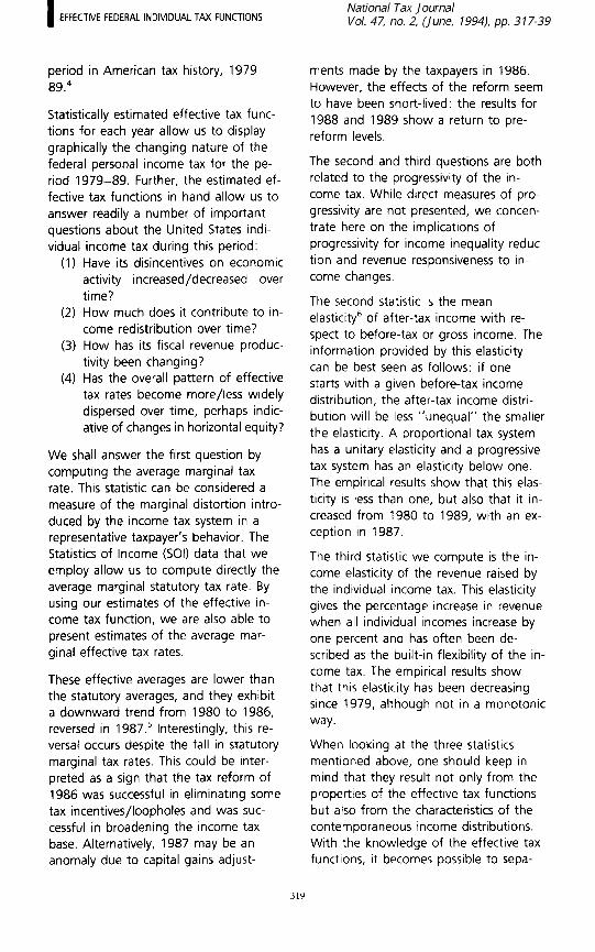
All coefficients are sigqificant at the usual fiviz perc:ent confidence level. The R2’s reported were computed from the SAS output files as one minus the ratio of weighted surn of re$idual squares di- vided by the corrected total weighted sum of c,quares. To prqvide a check on the adequacy of the fynctional form usecl, we also present the R2 of regressions wi1.h the same dqta using a fifth- order pclynomial on inicome (six parameters) in column [7] of Iable 1, R& The R2’s from our three-paiameter nonlinear regrlession are always s~ubstantially higher thar, these for the polynomials.” Later on, we will exarnine in more detail the

322


TABLE 1 STATISTICAL ESTIMATION RESULTS

Year

1979

1980

1981

1982

1983

1984

1985

1986

1987

1988

1989

;I rd1 ri 0.817 0.022 0.479

181,555 (.0041) (.OOOZ) (.0046) 0.558 0.346 0.829 0.023 0.455

149,215 (.0047) (.OOOZ) (.0044) 0.558 0.406 0.938 0.031 0.331

124,380 (.0075) (.0027) (.0027) 0.499 0.243 0.918 0.031 0.298

74,237 (.0095) (.0003) (.0032) 0.492 0.154 0.890 0.033 0.262

108,442 (.0084) (0003) (.0024) 0.445 0.142 0.899 0.029 0.262

71,766 (0118) (.0004) (.0036) 0.373 0.127 0.800 0.031 0.275

97,164 (.0084) (.0003) (.0034) 0.386 0.125 0.887 0.032 0.236

67,650 (.0134) (.0005) (.0031) 0.327 0.074 0.726 0.023 0.342

96,013 (.0072) (.0003) (.0055) 0.358 0.176 0.752 0.029 0.276

84,985 (.0081) (.0004) (.0035) 0.372 0.103 0.768 0.031 0.258

84,826 (.0114) (.OOOS) (.0041) 0.255 0.072

Standard deviations in parentheses.

evolution of the p’s and provide a possible interpretation for their decline.

In terms of interpreting the parameter estimates, we can see that the implied estimates of the intertemporal elasticities of substitution (l/l + p) fall between 0.51 and 0.58. These values are very similar to estimates from asset-pricing studies.18

As for b, the maximum effective tax rate, we see that it declined from the early to the latest years in our data. However, it is noteworthy that this rate increased from 1986 to 1987, despite the fall in the maximum statutory tax rates brought by the 1986 tax reform. This could be interpreted as a finding that the base-broadening efforts of the tax reform were successful. This issue will be discussed again in the next section.

INTERPRETATION AND APPLICATIONS

Chronological Comparisons

The estimated effective average tax functions are depicted in Figures 1

through 4. The tax functions were estimated with current income, but, for the purposes of making graphical comparisons meaningful, we adjusted for changes in the price level as measured by the Consumer Price Index, taking 1990 as the base year. The reader should also keep in mind that the results apply to the population of taxpayers with nonnegative taxes.

Visual inspection of these graphs reveals the principal finding that will be corrob- orated later in the paper with the calculation of average marginal tax rates and two average income elasticities. This finding is that the average tax rates for high incomes have been declining. This decline occurs even in years with no changes in statutory tax rates.

An exception to this trend is illustrated in Figure 1, which shows that from 1979 to 1980 there was a tax rate hike, statistically significantlg for incomes below $170,000. This was followed by a “twist” from 1980 to 1981, during

323

FIGURE 1. 1979.-81 Effective Average Taxes

1 --A--

i I 50 150 200

Income ($000)

which the tax rates decreased for higher income taxpayers but increased for others. Decreases in tax rates are statistically significant for incomes above $110,000, and increases in tax rates are statistically significant for incomes below $45,000.

There were no major changes in tax law during the 1979-80 period.20 Most likely, the principal reason for the finding reported above is that inflation pushed taxpayers up the bracket ladder, the infamous “bracket creep.”

The 1981 twist is due to the overall tax rate cut brought by the Economic Re- covery and Tax Act of 1981. This finding seems to confirm an idea advanced, among others, by Clotfelter (1984) that trying to counteract the effects of inflation on the tax system mainly by tax

cuts (as opposed to acti,ng through the adjustment of the zero-bracket or exemption limrit) tends to make the tax system less progressive.

Figure 2 traces the evolution of the effective tax function in the period between tax reforms, 198’1-85. Effective tax functions fall from 1981 to 1983, with statistically significant drops in both 1981-82 anid 1982-83. They stabilize in the period 1’983.-85, with no statistically significant changes. These results are not surprising since statutory tax rates declined during the early part of this pe- nod due to the Economic Recovery Tax Act of 1981, Also, we had a return to lower inflation levels.

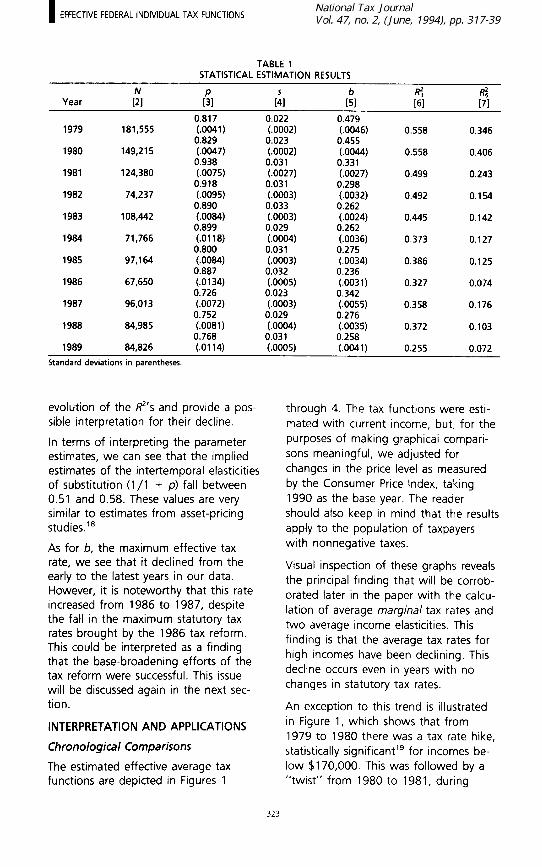
Examining Frlgure 3, we see that from 1985 to 1986, there is another fall in

324


FIGURE 2. 1981-85 Effective Average Taxes

I 50

I 100

Income ($000)

I 150

I 200

the effective tax function, no doubt a interpretation, in addition to the timing reflection of the massive realizations of effects on the realization of capital preferentially treated capital gains occur- gains, is that despite the cut in tax rates, ring in anticipation of the tax code income tax base broadening worked changes. However, the fall is only statis- quite effectively, with resulting increases tically significant for incomes above in effective rates. $145,000.

The Tax Reform Act of 1986 appears to be a second exception to the systematic trend noted above. Figure 3 documents that the effect of the Tax Reform Act of 1986 was to shift up the average effective tax function for higher income levels. In fact, tax rates fell for incomes below $75,000, although not in a statistically significant way, and increased for incomes above that threshold, with statistically significant increases for incomes above $145,000. One possible

However, the 1986 tax reform seems to have had only short-term effects in increasing effective rates for high incomes. According to Figure 4, the effective tax functions for 1988 and 1989 show a return to pre-reform levels. The 1989 effective average tax function is remarkably similar to the one for 1986, with no statistically significant differences for all income levels above $10,000.

It is worth noting that the changes shown in Figures 1 through 4 can be explained, at least partially, by the ability

325

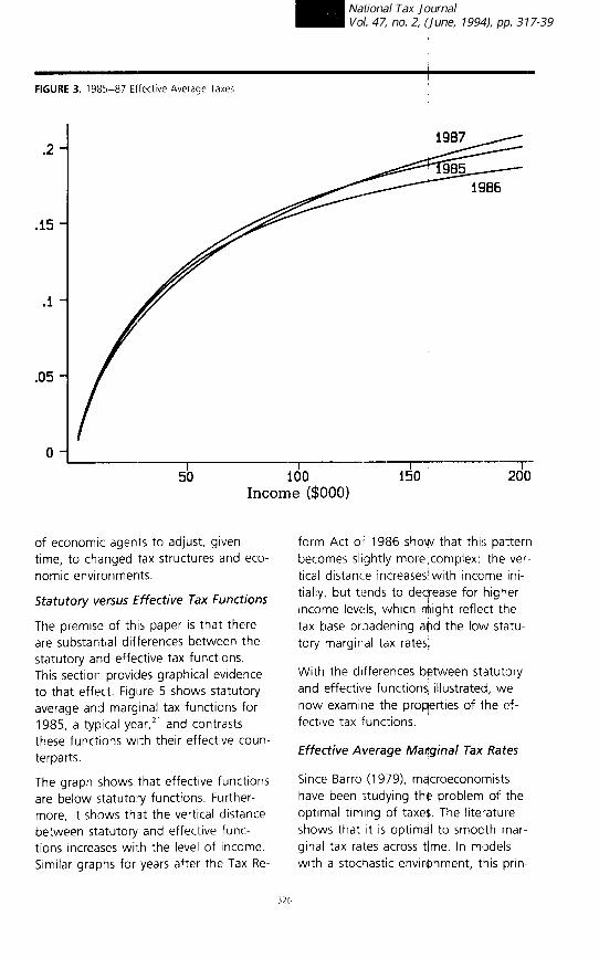
FIGURE 3. 1985-87 Effectw Average Taxes

.2 -

.15 -

.l -

.05 -

O-

------XL- Ido ----A------ 200 Income ($000)

of economic agents to adjust, given time, to changed tax structures and economic environments.

Statutory versus Effective Tax Functions

The premise of this paper is that there are substantial differences between the statutory and effective tax functions. This section provides graphical evidence to that effect. Figure 5 shows statutory average and marginal tax functions for 1985, a typical year,” and contrasts these functions with their effective coun- terparts.

The graph shows that effective functions are below statutory functions. Further- more, it shows that the vertical distance between statutory and effective functions increases with the level of income. Similar graphs for years after the Tax Re-

form Act 0. 1986 show that this pattern becomes slightly more complex: the ver.. tical distance Increases with income ini- tially, but tends to decrease for higher Income levels, which might reflect the tax base brl3adening and the low statutory marginal tax rates,

With the differences between statutory and effective .functions illustrated, we now examine the properties of the effective tax ‘unctions.

Effective Average Marginal Tax Rates

Since Barro (1979), macroeconomists have been jtudying the problem of the optimal timing of taxe$. The literature shows that it is optimal to smooth marginal tax rates across t/me. In models with a stocqastic environment, this prin-

326


FIGURE 4. 1987-89 Effective Average Taxes

.2 -

O- I 50 I 100

Income ($000)

I 150 I 200

ciple implies that marginal taxes follow a random walk.

Even without the motivation given by Barro’s theory, the average marginal tax rate seems of interest for several reasons. For economists trained in the tradi- tion of marginal reasoning, the so-called fiscal pressure (the ratio of total taxes to GNP) is not extremely informative of the degree to which the government affects the allocation of resources in an economy. Marginal tax rates seem to be a much more interesting variable to study.** The problem is that they are not found in the usual statistical sources.

In this section, we report our computations of the average marginal tax rate for the federal individual income tax, using the tax functions estimated previ-

ously. In the interpretation of our results, it is important to keep in mind that the evolution of average marginal tax rates is influenced but not perfectly controlled by government policy. Changes in demographics, industry, and occupational structures, etc. will also affect our find- ings. Our main purpose here is measurement rather than explanation, but later on we will briefly comment on the role of demographics.

The first issue that must be addressed is the determination of exactly what is the correct operational definition of the marginal tax rate. Is it the marginal tax rate computed from the effective income tax function or the statutory tax function? Seater (1982, 1985) argued in favor of the former, but Barro and Sahasakul (1983, 1986) defended the latter. Fortu-

327

FIGURE 5. 1985 Tax Functions

.6

.4

.2

0

Statutory. Marginal

I I 100 150

Income ($000)

I I w 250

nately, we are able to present computations for both types of average marginal tax rates. The statutory marginal tax is one of the variables in the SO1 data sets. Given a taxpayer’s income, our estimates of the tax function allovv us to estimate the corresponding effective marginal tax rate. The second issue that must be dealt with is aggregation. In the particular case of marginal tax rates, this means that there rnay be different averaging procedures that are desirable for different situations. To make this point more transparent, we illustrate it with two examples. The first example is labor supply. Suppose we are trying to estrmate an aggregate model of labor supply (e.g., a Lucas-Rapping model) and that we want to specify the correct net wages. What type of average of marginal tax

rates should we use? Absent prior knowledge about heterogeneity in labor- leisure preferences, a reasonable answer is that we should use s/mple averages of the rnarginal tax rates. hggregate labor supply is measured in terms of time allo- cated to work, and, in Iprinciple, all the agents in an economy have the same endowmlent of time.

For a given tax function fly) and a population of taxpayers i = 1, . . . N, average tax revenue is

[El r? = c t(y,)lN.

Similarly, we can define the average marginal tax as

328


MTSA = 2 t’(y,)/N ,= 1

where MTSA is the simple average marginal tax and t’(y) is the marginal tax rate as a function of income.

The second example is saving. On average, agents with higher incomes save more. If we include a marginal tax rate in a model explaining aggregate saving, it seems reasonable to use an income weighted average marginal tax rate. This is generally considered to be the most relevant operational definition of the concept of average marginal tax rate. Using an optimal growth model, Easterly and Rebel0 (1993) prove that this income weighted rate is the statistic summarizing the fiscal system that appears in the equation determining an economy’s growth rate. Formally, this income weighted average marginal tax is given bY

q

The effective marginal tax functions used come from the estimates of equation 1 :

P' (y) = &I - (j + y-i)(-1/4-1) *y-l-P),

where the “hats” denote statistical estimates of the parameters.

In Table 2, we present our estimates of the four types of average marginal tax rates.23 Table 2 points to a declining trend for almost all effective marginal rates considered. There are two major exceptions when the income weighted

tax rates have gone up. The first exception is the increase from 1979 to 1980, for which we have already advanced bracket creep as the explanation. The second exception is the increase in the effective income weighted rate after 1986 to 1987, no doubt an effect of the 1986 Tax Reform Act.24 The results for 1988 and 1989 point to a return to the declining trend mentioned above. Notice also that the effective un- weighted rate has been declining since 1981.

Effects on the After-Tax Income Distribution

Effective tax function estimates can be used to provide measures of the impact on the distribution of net income of the tax system. A simple measure was suggested by Musgrave and Thin (1948) and studied by Jakobssen (1976) and Pfingsten (1986), among others: the elasticity of after-tax income x = y - t(y) with respect to gross income y, also called residual income elasticity.

According to Jakobssen (1976), this elasticity evaluated at a given point provides a local measure of the distributional effects of the income tax. A tax system in which this elasticity is everywhere below one generates an after-tax income distribution that Lorenz dominates the before- tax income distribution. An elasticity smaller than one also implies a progressive tax system, i.e., one in which average tax rates increase with income. The lower the elasticity, the larger the equalizing effects on the distribution of income.

An intuitive explanation of why this elasticity measures the equalizing effect of the income tax system relies on the notion that a tax with an elasticity less than one compresses the income distribution, in the sense that all agents have incomes “closer together” after taxes are paid. A statistical illustration of the

TABLE 2 AVERAGE MARGINAL TAX RATES

Year Statutory Effective Statutory Effective

Simple Rate Simple Rate Weighted Rate Weighted Rate

1979 0.226 0.167 0.302 0.222 1980 0.236 0.17ci 0.317 0.231 1981 0.246 0.17:; 0.331 0.223 1982 0.224 0.158 0.300 0.202 1983 0.206 0.142 0.281 0.182 1984 0.195 0.134 0.274 0.177 1985 0.200 0.134 0.278 0.176 1986 0.199 0.133 0.287 0.173 1987 0.181 0.132 0.244 0.184 1988 0.177 0.130 0.238 0.177 1989 0.178 0.131 0.238 0.174

concept can also be provided The standard deviation of the logarithms of in-- come is a commonly used measure of inequality. Then, a tax system with a constant residual income elasticity of 0.9 leads to a ten percent reduction of inequality, according to the measure above, while an elasticity of 0.95 only reduces inequality by five percent.

Any aggregate measure of progressivity has the problem that it will generally hide variations In progressivity across income groups. However, it IS useful to have a single aggregate index allowing quick comparisons and a first look at the data. To meet those needs, Pfingsten (1986) proposed and axiomatlcally justi. fied the average of the individually calculated residual income elasticities as a global measure of the distributional effects of the income tax as a whole. To formalize this concept, consider a parameter 8 that multiplies all the y,‘s. The elasticity of after-tax income with respect to 8, evaluated at 8 .= 1, provides a convenient formulation of the residual income elasticity that we are looking for:

_ + 1 1 - Oy,) -___ Table 3 shows that the federal Individual Hz ,-%N(1 --fty,N income tax IS moving @ward less

TABLE f INCOME ELAS, ICITIES -___---- ---.

Elasticity of Revenue with

Residual Incomei Respect to Year Elasticity Income ---- 1979 0.928 '1.533 .' 1980 0.925 1.515 1981 0.928 '1.447 1982 0.936 1.430 1983 0.945 '1.403 1984 0.947 '1.412 1985 0.949 '1.394 1986 0.950 1.349 1987 0.949 1.416 1988 0.952 '1.357 1989 0.953 '1.349 ------ ----.

where $14,) ,jncf t’(y,) arg, respectively, the average and marginal tax rates.

1 he problem is that unliess an effective tax function is estimated and used, such measures WIII not be applicable: for each level of income, there is an interval of average tax rates we can observe In the data. Which one should we use for our computation? The iintuitive ansvver to this question is the mean. This corresponds precisely to the effective tax function estimate.

lhe second column in Table 3 presents our computations of thp average elasticity.

330


compression of after-tax incomes. The Tax Reform Act of 1986 causes an inter- ruption in that movement. However, after a minute decrease in 1987, the elasticity returns to its previous upward trend in 1988 and 1989. To get a quan- titative idea of what these estimates mean, one can do a “back of the enve- lope” calculation, using the standard deviation of the logarithms of income as a measure of inequality and the assump- tion that the elasticity is approximately constant at all income levels. This allows us to say that the income tax reduced inequality by about 7.5 percent in 1980 but only by 4.7 percent in 1989.

Revenue Elasticities

From the perspective of an administra- tion preparing a budget, the effective tax function can be seen as a production function, mapping from an input set (the distribution of incomes) to revenues. Naturally, questions about input produc- tivity arise. The simplest of such questions is to study the marginal relation between aggregate income and revenue. Waldorf (1967), Pechman (1973), and Fries, Hutton, and Lambert (1982) among others examined this relation at an aggregate level.

We are interested in computing the elasticity of fiscal revenue with respect to income. We can use the technique employed in equation 7, and define such elasticity as the elasticity of R- with respect to 8:

dt? 8 N -T= c h$, t(vJ

deR ,=, R-N

where Ett,y,) = dtiJ/dy, v,/W is the elasticity of the tax function with respect to income evaluated at each taxpayer’s income level. The aggregate elasticity is thus a weighted average of the individual elasticities, where the weights are

the tax payments. Thus, this elasticity is necessarily greater than one for progressive tax systems. This last fact implies that inflation increases fiscal revenues in real terms, a phenomenon widely discussed in more inflationary times and known as bracket creep, which, as we have seen, was probably the single most important force affecting income taxation in the early years of our sample.

The income elasticity of fiscal revenue is of obvious importance when calculating revenue forecasts. Given a tax structure, governments preparing budgets would like to know how projected changes in the price level and in real incomes affect fiscal revenue. A naive way to handle the problem is to use the statutory marginal tax rates to compute the changes in revenues associated with individual income changes. However, this method neglects the simple fact that the effective marginal tax rates are different from the statutory tax rates. After all, if the income of a taxpayer increases, it is nat- ural for that taxpayer to adopt the tax avoidance behavior previously displayed by taxpayers in a similar situation. For this reason, it makes more sense (and it is a better budgeting procedure) to use effective income tax function estimates to perform this type of analysis.25

The last column in Table 3 shows our estimates of the elasticity of fiscal revenue with respect to the income distribution, computed by using our estimates for the effective tax function. The procedure followed to calculate the elasticities was straightforward: we computed the predicted tax revenue for the initial income distribution and for a second income distribution obtained from the first by multiplying all incomes by 1 .Ol. The percentage revenue change obtained is the elasticity.

We should point out that it would not be appropriate to use the estimates of

marginal tax rates, computed earlier, because they were designed with different purposes in mind. If data availability pre- cludes the use of the method employed above, the correct elasticity must be computed using a weighted marginal tax rate in which the weights are the total tax payments of each agent, as indicated above.26

The results in Table 3 point to a declining trend in the built-in flexibility of the individual income tax. This agrees with the overall decline in progressivity that occurred in the last decade.‘” Again, there seems to be a short-lived effect of the 1986 Tax Reform Act in 1987, followed by a return to the declining trend.

Changes in the Dispersion of Effective Tax Rates in the Tax System

As noted earlier, #one can see in Table 1 a decline in the 15”‘s of the regressions. This decline cannot be explained by a progressive inadequacy of the equal sacrifice tax functions, bec:ause the same decline in R”s is also present in the case of the polynomial regressions.

Here, we suggest that the mean squared error of tax regressions can be given a standard public finance interpretation. Horizontal equity typically refers to the extent to which taxpayers with the same characteristics are taxed in the same way. In a system with perfect horizontal equity, if we specify a regression with the correct functional form and take as explanatory variables the characteristics deemed relevant for equity purposes, perfectly measured, there should be no regression residuals. All taxpayers with the same ability to pay (and same additional characteristics) would pay exactly the same taxes. The extent to which the tax system departs frorn this extreme case can be quantified by the MSE of the regression.28

In the case of our analysis, the ideal

conditions mentioned bbove are not met. Despite our efforts, we cannot claim to have perfect income measures, and the regressions p

come).“’

For these reasons, we do not consider our MSEs to be rigorous measures of the levels of horizontal inequity. How- ever, if the reader is yilling to accept the income measures s reasonable and that the distribution o P need or demographic characteristics ,of the population does not change materially every year, then fluctuations in the MSE can be viewed as Indicative of the direction of change in the horizontal equity properties of the tax system.@

Table 4 includes the LjlSE of the regressions, the mean and standard deviations of household size, and the mean and standard deviation of a variable that measures one possible “needs” characteristic of the taxpayer population: the number of exemptions (other than age or blindness) claimed on each tax re- turrl.3’

An inspection of Table 4 reveals familiar facts: mean household size in the United States has been declinling and so has the household size standard deviation. SomethIng similar happens to the average nurnber of exemptions claimed by tax return.

Here, we should notice that the largest fall in the number of exemptions oc- cured in 1987, after the 1986 reform made it necessary to provide a social security number for each exemption claimed. Remarkably, 1987 is also the only year where household heterogeneity increased, as measured by the standard deviation of hou$ehold size. Except for 1987, we then find a smooth evolution of household composition, incapa- ble of explaining the 4 hanges in the


TABLE 4 HORIZONTAL EQUITY RESULTS

Number of Exemptions Household Size

Year Mean Std. Dev. Mean Std. Dev.

1979 2.367 1.443 2.294 1.514 1980 2.353 1.435 2.237 1.496 1981 2.328 1.420 2.178 1.476 1982 2.315 1.409 2.168 1.472 1983 2.306 1.401 2.162 1.470 1984 2.229 1.332 2.100 1.449 1985 2.219 1.312 2.056 1.434 1986 2.196 1.306 2.028 1.424 1987 2.085 1.401 2.015 1.419 1988 2.066 1.385 2.004 1.416 1989 2.037 1.373 1.940 1.393

Sources: Statistical Abstracts of the United States and calculations from the SOL

MSEs of the regressions to which we now turn.

The early years in our data have, on average, lower MSEs, which may suggest that horizontal inequity has been on the rise. In fact, there are fluctuations that make this only a tentative conclusion. The results for 1987-9 are particularly surprising, because they point to growing horizontal inequity after the Tax Re- form Act of 1986. But the decline in the MSE from 1986 to 1987 shows that the direct impact of the reform was benefi- cial. This is even more surprising when the parallel increase in the standard deviation of exemptions is taken into account

In order to establish the robustness of these results, we estimated separate effective tax functions for the two main types of tax filing units: single and married filing jointly. The results can be seen in Table 5, which also includes columns with the P’s of the matching fifth-order polynomial regressions, R$

The results of this disaggregated analysis are essentially the same as those obtained for all filers. The rank correlation coefficients between the MSEs in Table 4 and the MSEs in Table 5 is 0.95 for single and 0.91 for married filing jointly.

Regression MSE

0.0019 0.0020 0.0025 0.0021 0.0020 0.0027 0.0023 0.0030 0.0027 0.0023 0.0040

As before, the earliest years in the sample have the lowest MSEs, with fluctuations thereafter, a fall in the MSEs from 1986 to 1987 and an increase from 1988 to 1989.32 All in all, these results, though by no means definitive, point to a negligible role of changes in the demographic characteristics of the taxpayer population in explaining the changes in the MSEs of the tax regressions.

The question of what are the forces underlying these changes is outside the scope of this paper (hence, the word “exploratory” in the title of the paper), but we cannot help but advance the hypothesis that these changes may be related to genuine movements in horizontal inequity caused by, among other things, nonuniform intensity in the use of tax avoidance strategies.

Conclusions and Suggestions for Future Research

In this paper, we present estimates of the effective income tax functions for the federal individual income tax for 1979 to 1989. A simple functional form, based on theories of equal sacrifice, proves to handle the data in a satisfac- tory way despite the nonlinearities intrin- sic to the relation between income and taxes.

333

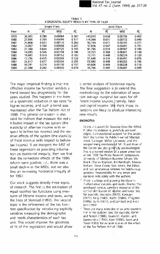
TABLE 5 HORIZONTAL EQUITY RESULTS BY TYPE QF FILER

Single Filers Joint Filers

Year N R: MSE RZ, N R: MSE R’6 1979 30,901 0.780 0.00084 0.367 143,010 0.658 0.00156 0.405 1980 27,995 0.765 0.00099 0.517 114,364 0.651 0.00172 0.449 1981 25,868 0.651 0.00175 0.264 92,194 0.611 0.00192 0.271 1982 13,067 0.740 0.00098 0.297 57,856 0.547 0.00201 0.151 1983 21,160 0.644 0.00125 0.16s 81,796 0.510 0.00187 0.195 1984 14,095 0.546 0.00158 0.188 53,725 0.398 I 0.00301 0.144 1985 19,681 0.553 0.00152 0.18;! 72,751 0.448 ' 0.00224 0.129 1986 12,756 0.435 0.00249 0.122 51,648 0.376 0.00297 0.076 1987 26,517 0.477 0.00204 0.205 63,680 0.448 0.00252 0.196 1988 19,791 0.574 0.00130 0.157 60,606 0.449 0.00228 0.119 1989 22,398 0.282 0.00450 0.078 56,766 0.390 0.00287 0.099

The major empirical finding is that the effective income tax function exhibits a trend toward less progressivity for the years studied. This happens in the form of a systematic reduction in tax rates for higher incomes, and such a trend was maintained after the Tax Reform Act of 1986. This general conclusion is also valid for indexes that measure the redistributive impact of the tax systern (the elasticity of after-tax income with respect to before-tax income) and the revenue effects of the system (the elasticity of fiscal revenue with respect to beforc- tax income). If we interpret the MSE of

these regressions as providing informa. tion on horizontal inequity, then we find that the immediate effects of the 1986 reform were positrve, i.e., there was a small decline in the MSEs, but we also find an increasing horizontal inequity after 1987.

Our work suggests directly three topics of research. The first is the estimation of equal sacrifice tax functions using measures of lifetime income and taxes, along the lines of Slemrod (1992). The second topic is the refinement of the tax function specification by introducing explicitly variables measuring the demographic and needs characteristics of each tax unit. This would improve the goodness of fit of the regressions and would allow

a better analysis of horizontal equity. The final suggestion is Jto extend this methodology to the estimation of separate average marginal {ax rates for different income sources, ~ namely, labor and capttal income. We think these ex- tensions are likely to produce interesting new results.

ENDNOTES

Financal support for Gouveia from the Alfred P. Sloan Foundation is gratefully acknowledged. Computational s pport for this project from the Center for Pub ic ‘; Fnancial Manage- ment, Carnegie Mellon University, and the programmrlng assistance lof Mr. Stuart Hiser elf the Celqter are also grat fully acknowledged. This IS a revised version f a paper presented at the 1993 Tax Policy esearch Symposium, Uiiiversity of Michigan B siness School. We thank Charles Boynton, III Randolph, Marcus Berllant, Steve Coate, I B ,b Inman, the Editor, and two anonymous referees for helpful sug- gestiors. Responsibility for any errors and opinions rests solely with the authors.

’ There IS a ilarge and gro mathematical statistics a d developed various sum ary measures of the

,,::

ing literature in public finance that

vertical distribution of income and taxes. See, for example, Atkinson ( 970), Kakwani (1977), King (1983), 1 Kie er (1984), Pfingsten (1986), Suits (1977), and Lambert and Aron- son (1993).

’ There are many examples of ex ante examina- tion of tax policies. See,, for example, Kiefer and Nelson (1986), Gramlich, l&ten, and Sammartino (199 1), Kern (1990), Scott and Triest (1993) for ex ante studies of the effect of the Tax Reform Act of 1986.

33-i


3 See National Research Council (1991, ch. 8): for a discussion of these issues.

4 For a lively account of the changes in tax policies in the 198Os, see Steuerle (1992).

’ The reversal occurs for the more important concept used: the income weighted average of the effective marginal tax rates.

6 Mean elasticities may obscure variation across income groups, but they provide a summary measure helpful in performing chronological comparisons.

’ Appendix A explores in more detail the advantages of using a fitted regression line vis- a‘-vis the raw data.

* The SOI publicly disseminates these data on magnetic tapes in a variety of ways: directly through the 501, through the National Ar- chives, and through the Office of Tax Policy Research, Graduate School of Business, Uni- versity of Michigan. Data tapes were obtained from Michigan for years 1979-86 and from the 501 division of the IRS for the years 1987 and 1988. The SO1 data for 1989 was provided by the National Bureau of Economic Re- search on a CD-ROM, which NBER prepared on behalf of the SO1 for members of the 501 Advisory Board, of which Strauss is a mem- ber.

’ This category consists of nonmarket income (production for self-consumption, services of owner-occupied housing, etc.) and excluded income (some types of cash and noncash transfer income, interest on state and local bonds, and unrealized capital gains).

lo See Pechman (1983 and 1985, pp. 1 l-14). ” The income concept used averages 57 per-

cent of GNP, 71 percent of national income, and 81 percent of personal income concept in the national income accounts, net of government transfer payments. See Berliant and Strauss (1985, 1991) for more details.

l2 AGI excludes a substantial portion of the capital gains, interest, pensions, Social Security benefits, unemployment compensation, and other income actually reported on tax returns. Furthermore, there are IRA and Keogh exclusions, exclusions for working couples, etc. All of these are included in the analysis.

l3 There is no advantage in including very low incomes in the analysis, because our estimates of the effective tax function are likely to be biased for very low incomes, given that we lack information on nonfilers. However, that omission should not be a serious problem for most of the income distribution range.

l4 With this specification, the asymptotic average and marginal tax rate is b * 100 percent.

15

16

17

18

19

20

21

22

23

24

25

26

27

28

Charles Boynton suggested it could be interpreted as the maximum politically feasible tax rate See Johnston (1984, p. 353). Standard results in sampling theory (Neyman’s allocation) suggest higher sampling rates for strata with higher variances. In that case, the optimal correction for heteroskedasticity is to run regressions weighted by the inverse of the sampling rate. We interpret the fact that this correction works as evidence that optimal stratification procedures were followed. Notice that the p’s are for average tax functions. The matching R2’s for total tax regressions are much higher, but these specifica- tions lead to heteroskedasticity problems. See, for example, Hall (1988). The nonlinear least-squares parameter estimates are asymptotically normal (see Judge et al. (1985, p. 199). That allows us to use a Taylor expansion of the regression equation to perform significance tests on the dlffer- ences of predicted average tax rates for different years, conditional on a given real income level. The significance statements refer to tests carned at 95 percent confidence and applied to incomes up to $250,000 (at 1990 prices). See Pechman (1987, p. 318). The statutory taxes apply to a married couple with two dependents filing jointly. We do not take the earned income credit into account, and we assume the couple claims the standard deduction. For example, deadweight losses depend on the square of the marginal tax rate. If the average tax rates underestimate the marginal tax rates, the problem is compounded when trying to get a measure of excess burden. All estimates in Tables 1 through 6 use sampling weights so as to replicate the overall population of taxpayers. The average tax rate decreased in 1987, because the tax reform increased exemptions substantially. Except for those that no longer pay taxes, this change had little direct effect on marginal tax rates and that effect was more than compensated by base broadening for higher incomes. The results of this exercise could be useful to check revenue forecasts produced by more sophisticated models taking into account the endogeneity of credits and deductions. On this point, see also Auerbach (1988). Elasticity values are lower than the forecasts In Pechman (1983). This measure has an obvious visual appeal.

335

See Paglin and Fogarty (1972) for an early ap- plication of this approach.

2g Additionally, there is the problem of how to account for differences in needs across taxpaying units. For example, in the case of fam- ily size, the standard procedure in most tax systems is to have a variable number of exemptions. However, the standard procedure in economic analysis for taking household stze into account is quite different, relying on the use of equivalence scales. See, for example, Slesnick (1993).

3o Note also that, since the dependent variable is an average rate, the MSE does not depend on the units of measurement for income and taxes and, in particular, on changes in the price level.

3’ Exemptions for age and blindness were sub- stituted by other tax code provlsions after the 1986 tax reform.

32 The 1989 MSE for singles is comparatively high, Further disaggregation, in itemizers and nonitemizers, shows that the MSEs for both groups remain high. We have not found a simple explanation for these results.

33 The results here used the same sarnple and definitions as those used in the estimation of the effective tax functions

34 Not shown but available from the authors.

REFERENCES

Arrow, Kenneth 1. “Microdata Simulation: Cur- rent Status, Problems, Prospects.” In Microeco- nom/c Simulation M#odels for PO/ICY Analysis, edited by R. Haveman and K. Hollenbeck. New York: Academic Press, 1980.

Atkinson, Anthony B. “On the Measurement of Inequality,” Journal of Economic Theory 2 (1970): 244-63. Auerbach, Alan 1. “Capital Gains Taxation in the United States: Realizations, Revenue and Rhetoric.” Brooking:; Papers on Economic Activity 2 (1988): 595-631. Barro, Robert. “On the Determination of Public Debt.” Journal of Political Economy 87 (1979): 940-7 1. Barro, Robert and Chaipat Sahasakul. “Mea- suring the Average Marginal Tax Rate from the Individual Income Tax.” Journal of Business 56 (1983): 419-52 Barro, Robert and Chaipat Sahasakul. “Aver- age Marginal Tax Rates from Social Security and the Individual Income Tax.” JOUrnJ/ of Business 59 (1986): 555-66.

Berliant, Marcus C. and Miguel Gouveia. “Equal Sacrifice and Incentive Compatible In-

come Tar.ation.” Journal of Public fconom/cs 51 (1993): 219.-40.

Berliant, Marcus C. and pobett P. Strauss. “The Horizontal and Vertiqal Equity Characteris- tics of thle Federal lndividu I Income Tax, 1966-. 77.” In Horizontatal Equity, “u ncertainty, and fco- nomic Well-Being: Proceedings of the 1983 NBER Conference on Income and Wealth Chi- cago, edited by M. David #nd T. Smeeding, Unl- versrty of Chicago Press, 1885. Berliant, Marcus C. and hobert P. Strauss. “Horizontal ,qnd Vertical E uity: A Theoretical Framework and Empirical $ esults for the Federal Indivldua: Income Tax 196b--87.” University of Rochester Economic Reseafch Institute Working Paper, 1991 Clotfelter, Charles. “Tax Cut Meets Bracket Creep: The Rise and Fall of Marginal Tax Rates, 1965-l 984.“ Public Finance Quarter/y 12 (1984): 131 .52. Easterly, William and Sqrgio Rebelo. “Mar- ginal Income Tax Rates aniJ Economic Growth in Developing Countries.“fuqopean Economic Re- vievv 37 (1993): 409-l 7. Fries, Albert, John P. Hu(tton and Peter J. Lambert. “The Elasticity df the U.S. Individual Income lax: Its Calculatioq, Determinants and Behavior ” Review of fcoflomics and Statistics 64 (1982): “47..55. Gramlich, Edward, Rich rd Kasten, and Frank Sammartino. “Growing I I equality in the 1980’s: The Role of Federgl Taxes and Cash

Transfers,” In Uneven rid+: Rising inequality in the 1980’s, edited by 5. Danziger and P. Gott- schalk. New York: Russell Sage, 1993. Hall, Robert. “lntertempdral Substitution In Consumption.” Journal of Political Economy 96 (19138): 339 -57. Jakobssen, U. “On the Measurement of the De- gree of Progression.” Jo&al of Public fconom- its 20 (1976): 161-68. ~ Joint Committee on Ta ation. Methodology and Issues i/i Measuring :! hanges in the Distribu- tion of 7bx Burdens. U.S. Kongress (IS-7-93), 1993. Johnston, John. Econometric Methods. New York; McGraw-Hill, 1984. Judge, Geokge, William Griffiths, Robert Hill, Helmut Lutkepohl, and . Lee. The Theory and Pra(rtice of Econometrics, : nd Ed. New York: Wiley, 1985, Kakwani, Nanak. “Meas rement of Tax Pro- gressivity: An Internation I Comparison,‘” The fconom/c Journal (1977) Q l-80. King, Mervyn A. “An Inqex of Inequalily. With Applications to Horizontal 1 Equity and Social Mcr- bilily.” Lconometrica 51 ( 983): 99-l 15.


Kern, Beth B. “The Tax Reform Act of 1986 and the Progressivity of the Individual income Tax.” Public finance Quarter/y 18 (No. 3, 1990): 259-72. Kiefer, Donald W. “Distributional Tax Progres- sivity Indexes.” National Tax /ourna/ 37 (Decem- ber, 1984): 497-513. Kiefer, Donald W. and Susan Nelson. “Distri- butional Effects of Federal Tax Reform.” In Pro- ceedings of the 79th Annual Conference, Hart- ford, CT: National Tax Association-Tax Institute of America, 1986. Lambert, Peter 1. and J. Richard Aronson. “Inequality Decomposition Analysis and the Gini Coefficient Revisited.” Economic Journal (Sep- tember, 1993): 1221-27. Musgrave, Richard A. and Tun Thin. “Income Tax Progression: 1929-1948.” Journal of Politi- cal Economy 56 (1948): 498-5 14. National Research Council. Improving Informa- tion for Social Policy Decisions, The Uses of Mi- crosimulation Modeling. Washington, D.C.: Na- tional Academy of Sciences Press, 1991. Paglin, Morton and Michael Fogarty. “Equity and the Property Tax: A New Conceptual Fo- cus.” National Tax Journal 25 (1972): 557-66. Pechman, Joseph A. “The Responsiveness of the Federal Individual Income Tax to Changes in Income.” Brookings Papers on Economic Activity 2 (1973). Pechman, Joseph A. “Anatomy of the U.S. In- dividual Income Tax.” In Comparative Tax Stud- ies: Essays in Honor of Richard Goode, edited by 5. Cnossen. Amsterdam: North-Holland, 1983. Pechman, Joseph A. Who Paid the Taxes? 1966-85. Washington, D.C.: The Brookings In-

stitution, 1985. Pechman, Joseph A. Federal Tax Policy (5th ed.). Washington, D.C.: The Brookings Institu- tion, 1987. Pfingsten, A. The Measurement of Tax Progres- sion. Berlin: Springer-Verlag, 1986. Sahasakul, Chaipat. “The U.S. Evidence on Op- timal Taxation over Time.” Journal of Monetary Economics 18 (1986): 251-75. Scott, Charles E. and Robert K. Triest. “The Relationship between Federal and State Individ- ual Income Tax Progressivity.” National Tax Jour- nal 46, 2 (June, 1993): 94-108. Seater, John. “Marginal Federal Personal and Corporate Income Taxes in the U.S., 1909- 1975.” Journal of Monetary Economics 10 (1982): 361-81.

Seater, John. “On the Construction of Marginal Federal Personal and Social Security Tax Rates in the U.S.” Journal of Monetary Economics 15 (1985): 121-35.

Slemrod, Joel. “Taxation and Inequality: A Time-Exposure Perspective.” In Tax Policy and the Economy, Vol. 6, edited by James Poterba. Cam- bridge, MA: National Bureau of Economic Re- search, 1992. Slesnick, Daniel. “Gaining Ground: Poverty in the Postwar United States.” Journal of Political Economy 707 (1993): l-38. Steuerle, Eugene. The Tax Decade. Washing- ton, D.C.: Urban institute Press, 1992. Suits, Daniel B. “Measurement of Tax Progres- sivity.” American Economic Review 67 (1977): 747-52.

Waldorf, William H. “The Responsiveness of Federal Income Taxes to Income Change.” Sur- vey of Current Business (1967): 32-45.

Young, H. Peyton. “Distributive Justice in Taxa- tion.” Journal of Economic Theory 44 (1988): 32 l-35.

Young, H. Peyton. “Equal Sacrifice and Pro- gressive Taxation.” American Economic Review 80 (1990): 253-66.

Wooldridge, Steven. “Some Alternatives to the Box-Cox Regression Model,” international Eco- nomic Review 33 (1992): 935-55.

APPENDIX A: EFFECTIVE TAX FUNCTION ANALYSIS

COMPARED TO TABULATION OF RAW INCOME

AND TAX DATA

The tradrtronal analysis of the distnbutron of tax burdens, such as the classic work of Pechman (1985), relies on the tabulation of raw Income and tax data, with observations grouped by the deciles of the income drstnbution. This Appendix explains in more detail some of the advantages of using the statrstr- tally estimated effective tax function approach In- stead of the traditional tabulation methodology. To summarize, the effective tax function approach has

the following advantages: (a) it deals better with the nonlinearities in the tax functions (total tax functions are convex and average tax functions are con-

cave), (b) it overcomes methodological problems In the estimation of effective margrnal tax rates and

elasticities, and (c) It is easy to use to perform counterfactual analysts as well as statistical inference and testing.

We now elaborate on these points The objective of the analysrs is to summarize a large amount of In- formation In as few parameters as possible without

losing the essential features of the data. Our statrsti- tally estimated effective tax functron Implies that the effective Income tax schedule can be known accu- rately by knowing the values of three parameters In addition, the MSE and the variance-covanance ma-

337

trix of the coefficients (seven additional parameters) give the information needed to perform a variety of

statistical testing and inference.

However, let us here pursue the standard methodol-

ogy and see how one could use the raw income

and tax data to calculate the statistics reported tn this paper. We ~111 use such data for 1989 as an example. Results for other years are essentially the

same.

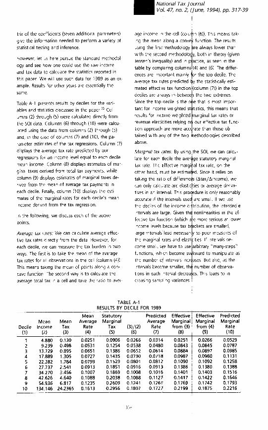
Table A-l presents results by declles for the variables and statistics dlscussed in the paper.33 Col-

umns (2) through (5) were calculated directly frorn the 501 data. Columns (6) through (IO) were calculated using the data from columns (2) through (5) and, in the case of columns (7) and (IO), the pa-

rameter estimates of tlbe tax regressions. Column (7) displays the average tax rate predicted by our

regressions for an income level equal to each decile mean Income Column (8) displays estimates of mar-

ginal taxes derived frown total tax payments, while column (9) displays estimates of marginal taxes de-

rived from the mean of average tax payments In each decile. finally, column (IO) displays the esti-

mates of the margtnal rates for each declle’s mean income derived from the tar. regresslon

In the followlng, we discuss each of the above points.

Average tax rates: We can calculate average effective tax rates directly from the data. However, for

each decile, we can measure the tax burden in two ways. The first is to take the mean of the average

tax rates for all observations In the cell (column (4)). This means taking the mean of potnts along a con-

cave function. The second way IS to calculate the average total tax in a cell and take the ratio to aver-

age income In the cell (colu$n (6)). This means taking the mean along a convei function. The results

using the first methodology Bre always lower than with the second methodolo y, both In theory (gtven Jensen’s Ineqljality) and in p actlce,

1 as seen in the

table by comparing columns (4) and (6). The differ-

ences are Important mainly for the top decile. The

average tax rates predlcted tjy the statistwcally estimated effective tax functioni(column (7)) in the top deciles are always in-betwee/-, the two extremes.

Since the top decile is the o

:

e that IS most impor-

tant for ircome weighted st tistlcs, this rneans that results for income weighted marginal tax rates or revenue elasticities relying 04 our effective tax func-

tlon approach are more accqrate than those obtained with any of the two hethodologies described

above.

MJ~~~vxI/ tax rates: By using the 501, we can calculate for each decile the averdge statutory marginal

tax rate. The effective margiiilal tax rate, on the other hard, must be estimakd. Since it relies on

taking the ratio of differences (Atax/Aincome), we can (only calculate arc elastic/ties or average deriva-

tives In an interval. This procedure is only reasonably accurate 1.f thf! intervals used are small. It we use the deciles of the income diitribution, the interdecile

Intervals are Idrge. Given thd nonlinearities in the effective tax function (which a/e more serious at lower

Income levels because tax b ckets are smaller), large intervals lead 1” necessari y to poor measures of

the marginal r’ates and elastifities. If Intervals become small, we have to use Iarbitrary “many-steps”

functions, which become a\hlkward to manipulate as the number of intervals incrdases. But also, as the

Intervals become smaller, th number of observations In each Interval decrea es. This leads to In- creasing sampling variances.

TABLE A-l RESULTS BY DECILE F0R 1989 __-___-- -----

Mean Statutorv Predicted Effective Effective Predicted Mean Mean Average Margina)

Decile Income Tax Rate Tax (1) (2) (3) (4) (5) --pm-

Average Marginal Marginal Marginal Rate from (3) from (4) Rate

(7) (8) (9) (10) ---A 1 4.880 0.130 0.0251 2 9.239 0.498 0.0531 3 13.729 0.895 0.0651 4 17.889 1.305 0.0727 5 22.282 1.784 0.0799 6 27.737 i! 541 7 3:456

0.0913 34.270 0.1007

8 42.626 4.640 0.1088 9 54.936 6.817 0.1235

10 134.146 24.2365 0.1613

0.0906 0.1254 0.1386 0.1435 0.1529 0.1851 0.1869 0.2038 0.2609 0.2956

0.0266 0.0538 0.0652 0.0730 0.0801 0.0916 0.1008 0.1088 0.1241 0.1807

-___

0.0314 0.0251 0.0266 0.0529 0.0480 0.0843 0.0845 0.0787 0.0614 0.0884 0.0897 0.0985 0.0718 0.0987 0.0980 0.1131 0.0812 0.1090 0.1092 0.1258 0.0913 0.1386 0.1380 0.1388 0.1016 0.1401 0.1403 0.1516 0.1127 0.1417 0.1422 0.1646 0.1261 0.1769 0.1742 0.1793 0.1727 0.2199 0.1875 0.2216


Another problem is that if we use data for deciles,

we do not have taxes and income at the bottom

and top of each decile allowing us to estimate the average marginal tax rate. What we have is only the

mean in each decile. One could redefine the inter-

vals over which we estimate the average marginal

rate, but that is not possible because of the top de- crle, where the upper limit would have to be infin-

ity. So, if we calculate marginal rates by taking dif-

ferences in Income and taxes for each cell and

starting at zero income and taxes, we get underestr-

mates of marginal tax rates. These results are shown

above by comparing columns (81, (9), and (IO). The underestimation problem IS then transmitted to the

calculation of the revenue and residual income elas-

ticities. With the statistically estimated effective tax

function, we can simply calculate at each income level the derivative of the function, which Implies

(assuming a good functional form ) greater accuracy

estimating marginal tax rates and elasticities.

Statistical inference: The statistically estimated effec-

tive tax function has well-known statistical proper-

ties that, for example, allow us to test for drffer-

ences In the average tax rates across years In any given Income range. This cannot be easily done with

other approaches. Wtth the tradrtronal analysis, It would be difficult to generate such results, not only due to the technology of statistrcal Inference but

also due to the more fundamental problem that differences in income distributions could not be ab-

stracted away.

APPENDIX B: HETEROSKEDASTICITY TESTS

We performed the Breush-Pagan test for heteroske-

dasticity. This heteroskedasticity test involves a linear

regression of the squared residuals on income and Income squared:

Res(atr)2 = cl + c2 y + c3 J + w

The test uses the fact that the quantity N x ti (where both N and R2 pertain to the regression

above) follows a x2 (2j under the null hypothesis of homoskedastrcrty. These auxiliary regressions34 have

an I?’ near zero in all cases, so we do not reject the null hypotheses of homoskedasticity.

effective federal individual income tax functions - national tax journal

Documents