Effective Load Carrying Capacity and Qualifying Capacity

Calculation Methodology for Wind and Solar Resources

Staff Proposal

Resource Adequacy Proceeding R.11-10-023

California Public Utilities Commission – Energy Division

January 16, 2014

Introduction

In compliance with Senate Bill (SB) 2 (1X), this Energy Division Staff Proposal (Proposal) recommends a

calculation methodology for the California Public Utilities Commission’s determination of the Effective

Load Carrying Capability (ELCC) and Qualifying Capacity (QC) of wind and solar resources. A resource’s

Qualifying Capacity (QC) is the number of Megawatts eligible to be counted towards meeting a load

serving entity’s (LSE’s) System and Local Resource Adequacy (RA) requirements, subject to deliverability

constraints.1

ELCC is a percentage that expresses how well a resource is able to meet reliability conditions and reduce

expected reliability problems or outage events (considering availability and use limitations). It is

calculated via probabilistic reliability modeling, and yields a single percentage value for a given facility or

grouping of facilities. ELCC can be thought of as a derating factor that is applied to a facility’s maximum

output (Pmax) in order to determine its QC. Because this derating factor is calculated considering both

system reliability needs and facility performance, it will reflect not just the output capabilities of a

facility but also the usefulness of this output in meeting overall electricity system reliability needs.

In accordance with the RA proceeding Scoping Memo (R.11-10-023), Energy Division (ED) staff issues this

Proposal and seeks formal comments. Party comments will inform the development of a Proposed

Decision, and will become part of the rulemaking’s record. Formal comments on this Proposal should be

emailed to the service list for the RA proceeding, R.11-10-023, on or before February 18, 2013. These

comments are to be filed and served.

It is noted that only the ELCC and QC methodology for supply-side wind and solar resources is within the

scope of this Proposal. “Solar resources” here includes both photovoltaic and solar thermal resources;

however, behind the meter resources are not considered. Flexibility and effective flexible capacity (EFC)

are also not within the scope of this document. The modeling upon which the ELCC and QC methodology

depends is described in a separate, companion staff proposal: Probabilistic Reliability Modeling Inputs

and Assumptions (Assumptions Proposal).2 The QC and EFC methodologies for energy storage and

1 The revised QC that incorporates deliverability constraints is called the Net Qualifying Capacity (NQC).

2 The most recent version of that proposal can be found at

http://www.cpuc.ca.gov/PUC/energy/Procurement/RA/ra_history.htm.

demand response resources are also addressed in a separate proposal: Qualifying Capacity and Effective

Flexible Capacity Calculation Methodologies for Energy Storage and Supply-Side Demand Response

Resources. It is not recommended that the QC and EFC methodologies for fossil-fuel resources be

modified at this time; any potential modifications are not within the scope of this Proposal.

While ELCC calculations have been conducted for conventional resource types since the 1960s and are

now also relatively well-understood for renewable resources, there can be some differences in

implementation. The extensive literature developing and documenting the ELCC concept for renewable

resources includes recent publications from the North American Electric Reliability Corporation (NERC),3

National Renewable Energy Laboratory (NREL),4 the IEEE Power and Energy Society,5 and the California

Energy Commission (CEC) Public Interest Energy Research (PIER) Program.6 Parties seeking more

detailed background on ELCC calculations and their usage in other jurisdictions are encouraged to

review these publications. This Proposal recommends one particular approach, and the primary purpose

of this Proposal is to solicit stakeholder feedback regarding the validity of this approach. However,

stakeholders with alternative proposals are invited to share these in their comments and to contact staff

regarding participation in forthcoming RA workshops.

Regardless of how the ELCC is calculated, it is ultimately a derating factor applied to the nameplate

capacity (Pmax) of a resource in order to determine its QC. Mathematically, this translates into the

following formula: QC = ELCC (%) * Pmax (MW).

The following sections outline the calculation methodology recommended by ED staff. The document

ends with a review of ELCC values for wind and solar resources calculated in other studies and

jurisdictions. Staff will also publish preliminary Energy Division modeling results in the coming month as

part of its effort to conduct transparent modeling and ELCC/QC calculations.

3 Methods to Model and Calculate Capacity Contributions of Variable Generation for Resource Adequacy Planning,

NERC, 2011. http://www.nerc.com/docs/pc/ivgtf/IVGTF1-2.pdf.

4 Summary of Time Period-Based and Other Approximation Methods for Determining the Capacity Value of Wind

and Solar in the United States, NREL, 2012. http://www.nrel.gov/docs/fy12osti/54338.pdf.

5 Capacity Value of Wind Power, NERC, 2011. http://www.nerc.com/docs/pc/ivgtf/ieee-capacity-value-task-force-

confidential%20(2).pdf

6 California Renewables Portfolio Standard Renewable Generation Integration Cost Analysis, the California Wind

Energy Collaborative, NREL, Oak Ridge National Laboratory (ORNL) and Dynamic Design Engineering, 2006.

http://www.energy.ca.gov/2006publications/CEC-500-2006-064/CEC-500-2006-064.PDF

Effective Load Carrying Capability (ELCC) Framework

ELCC reflects the contribution of a resource type towards meeting reliability needs

As previously mentioned, effective load carrying capability (ELCC) is an output of probabilistic modeling,

which assesses likely system needs and the potential for wind and solar resources to contribute to these

needs. The ELCC expresses how well the facility is able to meet reliability conditions and reduce

expected reliability problems or outage events caused by capacity shortfalls as compared to a perfect

generator (considering availability and use limitations).

ELCC can be viewed as matching the usefulness of a resource’s operating characteristics to reliability

conditions; for example, if modeling indicates that reliability needs are greatest in the afternoon, then a

resource that only operates in the morning would be derated more than an otherwise-identical resource

that only operates during the afternoon, because its contribution to reliability needs would be smaller.

Similarly, a resource with a high outage or underperformance rate at times of system stress would also

be derated more than an otherwise-identical, more reliable resource. For wind and solar resources,

monthly ELCC values are calculated to reflect seasonal variation in both generation profiles and system

needs. In order to conduct this assessment, modeling must encompass the complete electrical system,

from load forecasts to transmission constraints to generation forecasts, as shown in Figure 1.

A single ELCC will be calculated for groups of similar facilities

Proposed approach and groupings

The probabilistic reliability modeling is conducted using a program called SERVM, as described in the

companion staff proposal, Probabilistic Reliability Modeling Inputs and Assumptions (Assumptions

Proposal).7 This software allows every facility in the Western Electricity Coordinating Council (WECC) to

be modeled individually. As documented in the Assumptions Proposal, with the exception of

7 The most recent version of that proposal can be found at

http://www.cpuc.ca.gov/PUC/energy/Procurement/RA/ra_history.htm.

Figure 1. Factors considered in determining ELCC.

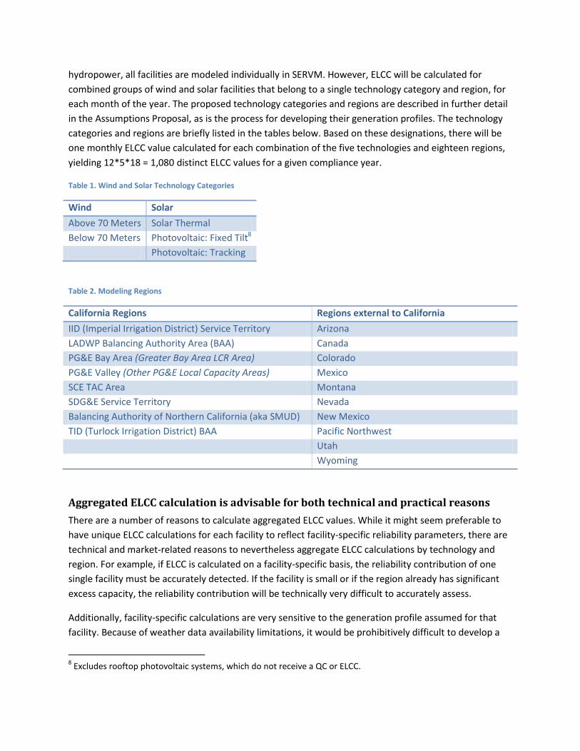
hydropower, all facilities are modeled individually in SERVM. However, ELCC will be calculated for

combined groups of wind and solar facilities that belong to a single technology category and region, for

each month of the year. The proposed technology categories and regions are described in further detail

in the Assumptions Proposal, as is the process for developing their generation profiles. The technology

categories and regions are briefly listed in the tables below. Based on these designations, there will be

one monthly ELCC value calculated for each combination of the five technologies and eighteen regions,

yielding 12*5*18 = 1,080 distinct ELCC values for a given compliance year.

Table 1. Wind and Solar Technology Categories

Wind Solar

Above 70 Meters Solar Thermal

Below 70 Meters Photovoltaic: Fixed Tilt8

Photovoltaic: Tracking

Table 2. Modeling Regions

California Regions Regions external to California

IID (Imperial Irrigation District) Service Territory Arizona

LADWP Balancing Authority Area (BAA) Canada

PG&E Bay Area (Greater Bay Area LCR Area) Colorado

PG&E Valley (Other PG&E Local Capacity Areas) Mexico

SCE TAC Area Montana

SDG&E Service Territory Nevada

Balancing Authority of Northern California (aka SMUD) New Mexico

TID (Turlock Irrigation District) BAA Pacific Northwest

Utah

Wyoming

Aggregated ELCC calculation is advisable for both technical and practical reasons

There are a number of reasons to calculate aggregated ELCC values. While it might seem preferable to

have unique ELCC calculations for each facility to reflect facility-specific reliability parameters, there are

technical and market-related reasons to nevertheless aggregate ELCC calculations by technology and

region. For example, if ELCC is calculated on a facility-specific basis, the reliability contribution of one

single facility must be accurately detected. If the facility is small or if the region already has significant

excess capacity, the reliability contribution will be technically very difficult to accurately assess.

Additionally, facility-specific calculations are very sensitive to the generation profile assumed for that

facility. Because of weather data availability limitations, it would be prohibitively difficult to develop a

8 Excludes rooftop photovoltaic systems, which do not receive a QC or ELCC.

production profile that is as accurate as would be required to yield improved results over aggregated

profiles; any inaccuracies could yield significant deviations in QC. Moreover, the process of coming to

consensus on what production profiles are appropriate for an individual facility would be much more

difficult than conducting the same process for aggregated production profiles.

The modeling and administrative burden of conducting facility-specific, monthly ELCC calculations would

also be significant. With most facility parameters modeled on a facility-specific basis (the notable

exception being generation profiles, the calculation of which is described in detail in the Assumptions

Proposal) and 1,080 distinct ELCC values already envisioned for each compliance year, staff believes that

grouping the ELCC calculations across five technologies and eighteen regions represents a reasonable

compromise between specificity and feasibility.

It is also important that QC values be relatively predictable, so that developers and LSEs can efficiently

respond to the market signal they provide. Grouping by technology category and region will enable

market participants to more easily assess what types of wind and solar projects will be most cost-

effective, while still providing a reasonably accurate indication of those resources’ contributions to

reliability.

Perhaps most importantly, however, facilities are grouped into categories due to the fact that resources

of a similar type contribute to reliability with diminishing returns, considered on an incremental basis; in

other words, one can imagine that the first solar facility that provides reliability benefit during the

middle of the day produces the highest marginal benefit, while subsequent solar facilities with the same

performance pattern produce a diminishing level of marginal benefit, as the need for capacity that time

has already been met. Wind facilities are less susceptible to the dynamic of diminishing returns due to

the higher variability of wind patterns across geographical distance, but the issue remains – subsequent

installations of similar technologies create diminishing returns.

However, in actual operations, there is no “first” facility providing reliability benefits in a given moment

– all of the facilities that are generating output are doing so simultaneously. Modeling a given resource

type in aggregate addresses the issue of marginal reliability contributions by in essence averaging the

aggregate reliability contribution across all facilities. This approach is also preferable to modeling

individual facilities while assuming that all other facilities of that type are already present, because that

approach would be equivalent to designating each and every facility modeled as the “last” facility to

come online – and thus the one with the lowest reliability contribution. Such an approach would

dramatically underestimate the total reliability contribution of the overall resource type.

Facilities will be compared to a “perfect generator”

There are three primary approaches to calculating ELCC:

1. Modeling reliability with and without a given resource type, and determining how much load

can be increased such that it cancels out the reliability improvement of including the resource.

2. Comparing the reliability impact of including the resource type to the reliability impact of

including a conventional resource with assumed operating and outage characteristics.

3. Comparing the reliability impact of including the resource type to the reliability impact of

including an idealized, “perfect generator”.

As previously mentioned, the approach recommended by staff is to compare the reliability contribution

of an actual resource type to that of a perfect generator. This is done to create a derating relative to the

maximum possible reliability contribution from a given MW of nameplate capacity, and to avoid

dependence on load and conventional generator assumptions. This approach is consistent with that

adopted in a recent NREL/GE Energy study, and a more detailed discussion of the reasoning behind this

choice can be found in that publication.9

A perfect generator is modeled as a facility with ideal operating characteristics: no transmission

constraints, immediate start-up and shut-down, infinite ramping capability, no use limitations, and no

outages. This generator has positive output only (no charging or dispatchable load). The comparison

concept is illustrated in Figure 2. The perfect operating characteristics are primarily modeled via the

standard unit inputs described in the Assumptions Proposal. However, the transmission constraints are

modeled by placing the perfect generator in its own modeling region, and by setting this region to have

no load and full deliverability to all other regions.

While it is only recommended that solar and wind resources receive QC in this manner for RA

compliance year 2015, fossil resources are also subject to a derating from the CAISO, reducing their

qualifying capacity to their “dependable” capacity. Fossil resources are also subject to the Standard

Capacity Product (SCP), which penalizes facilities that are not available for a sufficiently high percentage

9 Western Wind and Solar Integration Study, prepared for NREL by GE Energy, 2010. Note that the recommended

approach is referred to as “capacity value” in that document, while the term ELCC is used exclusively to refer to the

load-increasing approach. See Section 9, “Capacity Value Analysis” and specifically Section 9.5, “Comparison to

Other Measures”. http://www.nrel.gov/docs/fy10osti/47434.pdf.

Figure 2. ELCC calculations compare actual resource characteristics to an ideal generator

of Availability Assessment Hours;10 as a result, many fossil facilities will voluntarily reduce their QC to

account for factors such as reduced efficiency at high ambient temperatures. Moreover, all resources

are subject to CAISO deliverability calculations, which result in a net qualifying capacity (NQC). The NQC

is the value ultimately adopted by the CPUC as the capacity eligible to meet RA requirements.

ELCC calculations will consider all 8760 hours of the year

Because the modeling is probabilistic, many sample years are modeled in order to derive the expected

contribution of a given resource type. ELCC calculations consider reliability contributions during all of

these modeled hours. However, it could be possible to only consider contributions during the

Availability Assessment Hours currently utilized for assessing fossil fuel facilities. Alternatively, both

methodologies could be utilized and the higher of the two ELCCs applied to a given technology type and

region. Staff looks forward to parties’ comment as to which approach should be pursued.

Co-located storage will not be addressed at this time

In the Draft CPUC Energy Storage Use Case Analysis,11 On-Site Variable Energy Resource (VER) Storage is

defined as:

Energy storage that is located on-site of an intermittent resource such as wind and solar. These

storage deployments are used to enhance the capacity, energy, or ancillary services revenues of

that generator. Some technologies, such as batteries, may choose to operate a part of the

battery independently of the on-site generation source. That participation would be counted in

either the bulk storage system or ancillary services storage.

This storage will be modeled as a part of the WECC system in the reliability calculations, but will not be

considered to be operating in conjunction with the co-located wind or solar facility at this time. If the

storage independently meets RA eligibility criteria, then it may receive its own QC according to the rules

currently being developed for energy storage systems. If the storage does not independently meet RA

eligibility criteria, then it will not receive a QC value. In neither case will the storage facility influence the

QC of the on-site wind or solar facility. Treatment of co-located storage will be revisited for RA

compliance year 2016.

ELCC is calculated based on a monthly Loss of Load Expectation (LOLE) metric

Loss of load expectation is the amount of time during which system capacity is unable to meet system

load. For example, in a monthly LOLE calculation, if CAISO system load exceeds available generation for

10

For more information, see CAISO Tariff Section 40.9.3, Availability Assessment Hours for Standard Capacity

Product: http://www.caiso.com/Documents/ConformedTariff_Dec17_2013.pdf, page 929. For the availability

assessment hours starting in compliance year 2010, see Section 7.6:

http://bpmcm.caiso.com/Pages/BPMDetails.aspx?BPM=Reliability%20Requirements.

11 http://www.cpuc.ca.gov/NR/rdonlyres/3E556FDB-400D-4B24-84BC-

CD91E8F77CDA/0/TransmissionConnectedStorageUseCase.pdf

ten hours out of a total of 744 hours in the month, then the system LOLE for that month is equal to 10

hours ÷ 744 hours, or 0.013.

This metric enables system reliability to be compared across multiple scenarios and portfolio types. If

two model runs yield the same LOLE, then they are considered to have the same level of reliability, even

if the generation portfolio and causes of load shedding are very different. For example, if the model is

run once with 10 MW of wind in a given region (in addition to all other plants that make up the overall

generation fleet), and again with that wind replaced by 4 MW of natural gas combined cycle plants, and

both runs result in the same LOLE, then the two portfolios are considered to be equally reliable. It is

possible that the wind scenario is more likely to have load shedding during mid-day, while the natural

gas scenario is more likely to have load shedding in the early morning, but on the whole, the system

reliability is equivalent. Similar comparisons form the basis of the 1,080 ELCC calculations, as described

in the following section.

ELCC Methodology

The ELCC calculation requires modeling with a reliability calculator. As discussed above, this modeling

will incorporate the specific operating characteristics of each facility where possible (performance,

advance notice required, use limitations, Pmax and Pmin, etc.); however, the ELCC will be calculated as an

aggregate number for a given technology category, region, and month.

Conceptually, the ELCC for a given technology category, region, and month is a comparison of the

amount of generation capacity of that category and in that region to the amount of perfect generation

required to yield the same monthly LOLE, if the capacity in question is excluded from modeling. Note

that in order to create a derating factor (percentage below 100%), this relationship is inverted. This

comparison is illustrated in Figure 3.

For example, imagine there is 100 MW of fixed tilt photovoltaic solar capacity in a given region, and

modeling results show that the system LOLE for May is 0.001. If this solar capacity is removed from

modeling, system reliability would decrease and the May LOLE would increase, perhaps to 0.002. If 25

MW of perfect generation is required to bring the May LOLE back down to 0.001, then the ELCC would

be 25 MW / 100 MW = 25%. In other words, in the month of May, fixed tilt photovoltaic solar capacity in

the region in question improves system reliability 25% as much as the same nameplate capacity of

perfect generation.

ELCC Calculation

Each combination of technology category, region, and month requires a unique ELCC calculation. Let T

be the technology category in question, R be the region in question, and M be the month in question for

the calculation methodology detailed below.

1. Use a reliability calculator to model the WECC electrical system with all resources included, as

described in the Assumptions Proposal, and determine the loss of load expectation (LOLE) for

month M.

2. Model the system again, excluding all capacity of technology T in region R.

a. This will very likely increase the LOLE for month M, because there is less capacity available

to meet system needs. If it does not, then the capacity of technology T in region R does not

provide any reliability benefit in month M, at current levels. In other words, there is so little

of technology T installed in region R that its output is insufficient to prevent load-shedding

at times of system stress. In that case, the base case in step one needs to be modified to

simulate a level of penetration that is sufficient to create a measurable reliability benefit.

This can be accomplished by returning to step one and modeling additional capacity of T in

R. While this modified base case does not represent the actual system, it nevertheless

enables accurate calculation of the reliability impact of each incremental MW of technology

T in region R.

Figure 3. ELCC is based on a comparison of the actual and “perfect” capacities yielding identical LOLEs

3. Add a small amount of perfect generation12 capacity to the model, and recalculate the LOLE for

month M (continuing to exclude all capacity of T in R).

4. Repeat step three, stopping when the LOLE for month M is equal to that found in step one.

5. Define the ELCC of technology T in region R and month M to be equal to the total amount of

perfect capacity added upon completion of step four, divided by the total capacity of technology

T in region R (the sum of Pmax across all such facilities), as illustrated in Figure 4, below. Referring

back to Figure 3 above, this concept can be thought of as taking the MW capacity represented

by the “perfect generation” box on the right, and dividing it by the MW capacity represented by

the orange “technology T in region R” box on the left hand side. Because perfect generation by

definition has a greater contribution to reliability, less of it will be needed to yield the desired

LOLE. As a result, the numerator will be less than the denominator, and the ELCC will be below

100%.

Qualifying Capacity (QC) Calculation

As previously discussed, the ELCC percentage is a derating factor applied to the nameplate capacity

(Pmax) of a resource in order to determine its QC. While a monthly ELCC is calculated across all facilities

of a given technology and region in aggregate, it is applied to each individual facility to yield a facility-

specific QC, according to the following formula: QC = ELCC (%) * Pmax (MW).

In the future, it is possible that the QC or ELCC calculations could be modified to incorporate facility-

specific differences. However, that level of granularity is not under consideration for the 2015 RA

compliance year.

Review of ELCC Study Results from Other Agencies and Jurisdictions

While there are slight differences in ELCC methodologies across various studies, and while regional

differences significantly impact ELCC results (for example, regions that are windy during the day and

early evening are likely to have higher ELCCs for wind than regions where it is primarily windy at night),

it is nevertheless helpful to review existing literature and results. Several representative ELCC results are

reproduced below. As staff conducts its modeling, results will be compared with these values to ensure

reasonableness and understand the causes of any deviations from commonly accepted ELCC ranges.

12

Generation with ideal operating characteristics: immediate start-up, infinite ramping capability, no use

limitations, and no outages. Perfect generation has a Pmin of zero. It also has no transmission constraints.

Figure 4. ELCC is a ratio of the MW needed to provide identical LOLEs

California-specific ELCC Results

Both NREL and the CEC have conducted ELCC studies calculating wind and solar values that are specific

to California. Generally speaking, solar PV ELCCs range from about 60-75% at low penetrations (or

higher with natural gas backup), and decrease as penetration increases. This is because very high

penetration scenarios likely no longer face significant capacity shortfalls during times when solar PV is

generating. As penetration approaches 15%, the NREL findings shown in Figure 4, below, suggest that

the ELCC of fixed-tilt solar PV is likely to drop to roughly 44-52%, depending on orientation.

Table 3. Capacity credits calculated for the CEC PIER Program13

Resource Type

2002 ELCC 2003 ELCC 2004 ELCC

Relative

to peak

output

Relative to

nameplate

Relative

to peak

output

Relative to

nameplate

Relative

to peak

output

Relative to

nameplate

Solar PV with

auxiliary gas

generators

82% 88% 68% 83% 75% 79%

Wind:

Northern

California

33% 24% 37% 25% 44% 30%

Wind: San

Gorgonio

42% 39% 28% 24% 27% 25%

Wind:

Tehachapi

29% 26% 34% 29% 29% 25%

13

This analysis compares resources to conventional natural gas when calculating ELCC. Each year is a separate run

based on historical hourly generation data, and not a Monte Carlo simulation of many weather years. The report

can be found at http://www.energy.ca.gov/2006publications/CEC-500-2006-064/CEC-500-2006-064.PDF.

Figure 4. Solar photovoltaic (PV) ELCC values decrease with PV penetration in California: 2006 NREL study14

40%

45%

50%

55%

60%

65%

70%

75%

80%

0% 5% 10% 15%

Sola

r P

V E

LCC

Solar Penetration in California

Two-Axis Tracking

Southwest, 30° Tilt

Horizontal

South-Facing, 30° Tilt

Concentrating solar power (CSP) must be treated separately from solar PV, however, because it uses a

different technology. Its ELCC is also highly dependent on the sizing of the solar field relative to the

generation equipment (powerblock), a factor called the solar multiple (SM), with higher SMs yielding

higher ELCCs. CSP may also include significant onsite thermal energy storage, increasing dispatchability

and therefore improving a facility’s ELCC. NREL recently conducted a detailed study on methodologies

and considerations for calculating the ELCC of CSP facilities (Capacity Value of Concentrating Solar Power

Plants), and some of the results are reproduced below.15

14

Update: Effective Load-Carrying Capability of Photovoltaics in the United States, NREL, 2006.

http://www.nrel.gov/docs/fy06osti/40068.pdf.

15 Capacity Value of Concentrating Solar Power Plants, NREL, 2011. http://www.nrel.gov/docs/fy11osti/51253.pdf.

This study assumed parabolic trough technology (likely a lower bound when considering more flexible power

tower systems), and assumes CSP operators are able to forecast weather and price perfectly when optimizing plant

dispatch (creating slightly inflated values). It calculates capacity values via an ELCC calculation that compares CSP

facilities to a natural-gas-fired combustion turbine with an expected forced outage rate of 7%. Data are from 1998-

2005.

Figure 6. ELCC of CSP with thermal energy storage in Death Valley and Imperial Valley: 2011 NREL CSP study16

ELCC Results from Beyond California

For more extensive descriptions of capacity value studies and calculated ELCC values from across North

America, parties are encouraged to read the 2012 NREL report, Summary of Time Period-Based and

Other Approximation Methods for Determining the Capacity Value of Wind and Solar in the United

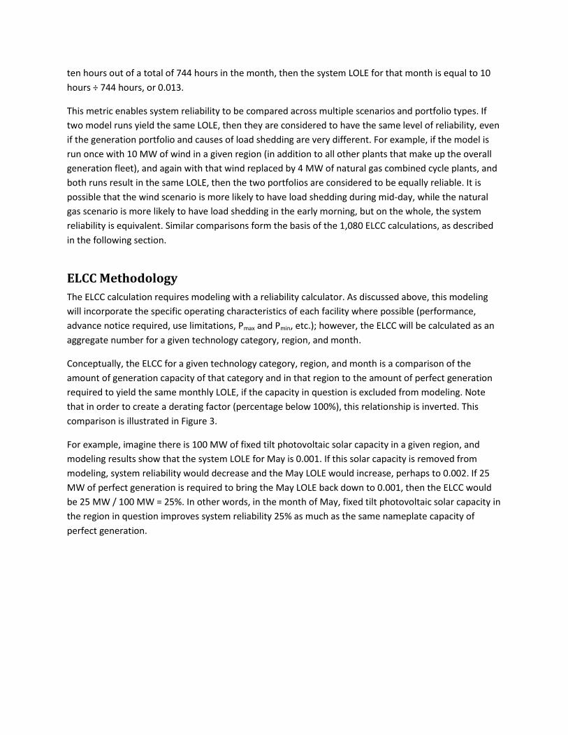
States; that report serves as the source for Table 5, below.

Table 5. Wind and solar capacity values in North America17

Region/Utility/Study ELCC Results Notes

APS (Arizona) South-facing, 45-47%

Southeast-facing, 33%

Averages based on loss of load

expectation (LOLE) simulations for

16

Capacity Value of Concentrating Solar Power Plants, NREL, 2011. http://www.nrel.gov/docs/fy11osti/51253.pdf.

These results are taken from NREL’s “energy and capacity market” scenario, because that scenario incorporates

more reliability-oriented dispatch optimization than the energy-only scenario. Data are from 1998-2005.

17 Source: Summary of Time Period-Based and Other Approximation Methods for Determining the Capacity Value of

Wind and Solar in the United States, NREL, 2012. http://www.nrel.gov/docs/fy12osti/54338.pdf.

Figure 5. Average ELCCs of CSP plants without storage, 1998-2005: 2011 NREL CSP study

Solar Multiple

ELC

C (

%)

Hours of Thermal Energy Storage

Dea

th V

alle

y EL

CC

(%

)

Hours of Thermal Energy Storage

Imp

eria

l Val

ley

ELC

C (

%)

Southwest-facing, 56%

Single-axis tracking, 70%

2003-2007.

BC Hydro 24% for on- and off-shore wind Used wind output-duration tables

based on synthesized

chronological hourly wind data for

different regions.

City of Toronto 23-37% for solar PV Garver ELCC approximation;

results depended on location,

orientation, and penetration level.

ERCOT 8.7% for wind Random data: no correlation

between wind and load.

Eastern Wind

Integration and

Transmission Study:

NREL/Enernex Corp

16.0-30.5% (with existing

transmission system) and 24.1-

32.8% (with a new transmission

overlay) for wind

Hydro-Québec 30% for wind Utilized a Monte Carlo simulation

that chronologically matched wind

and load data for a 36-year period.

Midwest ISO 12.9% in 2011 and 14.7% in

2012 for wind

New York: Solar Alliance

and the New York Solar

Energy Industry

Association

For solar PV, by penetration:

2%: 51-90%

10%: 51-74%

20%: 31-44%

PacifiCorp 8.53% for wind, but decreasing

with increasing installed

capacity

Utilized a sequential Monte Carlo

method to capture variation across

different weather years.

PSCO/Xcel (Colorado) Fixed-tilt PV: 59-63%

Single-axis tracking PV: 69-75%

Solar thermal parabolic troughs

without thermal energy storage:

68-81%

Based on 2004 and 2005 data at

three site locations.

Western Wind and Solar

Integration Study (AZ,

CO, NV, NM, and WY):

NREL/GE Energy

Wind: Between 10 and 15%, for

10-30% penetration

Solar PV: 25-30% at 1-5%

penetration

Concentrating Solar Power (CSP)

with 6 hours of thermal energy

storage: 90-95% at 1-5%

penetration.

Parties are encouraged to review

this extensive study in more detail.

See Section 9, available for

download at http://www.nrel.gov/

docs/fy10osti/47434.pdf.