Effectively Closed Sets of Measures andRandomness

Jan Reimann

January 12, 2007

Outline

Motivation

Measures and RandomnessOuter Measures on Cantor SpaceRandomness for Outer Measures

The Space of Probability MeasuresThe Weak TopologyEffective RepresentationsEffeczively Closed Sets of Measures

Hausdorff Measures and Probability MeasuresHausdorff MeasuresMass Distributions and Hausdorff MeasuresProving Frostman’s Lemma

MotivationHausdorff measures and probability measures

I Hausdorff measures are an indispensable tool in fractalgeometry: self-similar sets, rectifiability, dimension concepts.

I As measures, they are rather unpleasant to deal with: ingeneral not σ-finite, no integration theory, etc.

I Consequently, the study of sets of finite Hausdorff s-measureis very complicated.

I It is possible to “approximate” Hausdorff measures byprobability measures and make use their “good behavior”.

I Question: Can the theory of effective dimension, especiallythe connections to randomness and Kolmogorov complexity,contribute to this?

MotivationThe basic paradigm

random reals + Turing reductions = existence of measures

Measures on Cantor SpaceOuter measures from premeasures

Approximate sets from outside by open sets and weigh with ageneral measure function.

I A premeasure is a function ρ : 2<ω → R+0 ∪ {∞}.

I One can obtain an outer measure µρ from ρ by letting

µρ(X) = infC⊆2<ω

{∑σ∈C

ρ(σ) :⋃

σ∈C

Nσ ⊇ X

},

where Nσ is the basic open set induced by σ.(Set µρ(∅) = 0.)

The resulting µ = µρ is a countably subadditive, monotone setfunction, an outer measure.

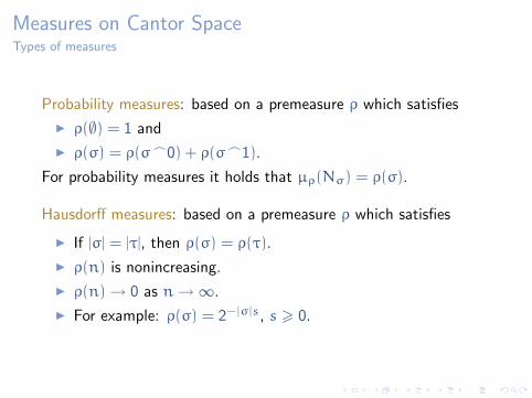
Measures on Cantor SpaceTypes of measures

Probability measures: based on a premeasure ρ which satisfies

I ρ(∅) = 1 and

I ρ(σ) = ρ(σ _0) + ρ(σ _1).

For probability measures it holds that µρ(Nσ) = ρ(σ).

Hausdorff measures: based on a premeasure ρ which satisfies

I If |σ| = |τ|, then ρ(σ) = ρ(τ).

I ρ(n) is nonincreasing.

I ρ(n) → 0 as n → ∞.

I For example: ρ(σ) = 2−|σ|s, s > 0.

Measures on Cantor SpaceNullsets

The way we constructed outer measures, µ(A) = 0 is equivalent tothe existence of a sequence (Wn)n∈ω, Wn ⊆ 2<ω, such that forall n,

A ⊆⋃

σ∈Wn

Nσ and∑

σ∈Wn

ρ(σ) 6 2−n.

Thus,

every nullset is contained in a Gδ nullset.

Randomness for Outer MeasuresEffective Gδ sets

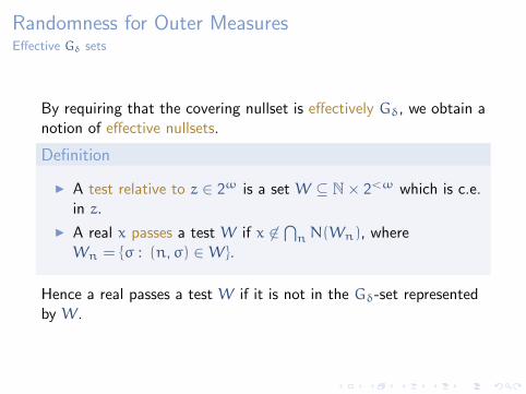
By requiring that the covering nullset is effectively Gδ, we obtain anotion of effective nullsets.

Definition

I A test relative to z ∈ 2ω is a set W ⊆ N× 2<ω which is c.e.in z.

I A real x passes a test W if x 6∈⋂

n N(Wn), whereWn = {σ : (n,σ) ∈ W}.

Hence a real passes a test W if it is not in the Gδ-set representedby W.

Randomness for Outer MeasuresMartin-Lof tests

To test for randomness, we want to ensure that W actuallydescribes a nullset.

Definition

Suppose µ is a measure on 2ω. A test W is correct for µ if for alln, ∑

σ∈Wn

µ(Nσ) 6 2−n.

Any test which is correct for µ will be called a test for µ.

Randomness for Outer MeasuresRepresentation of measures

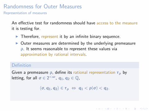
An effective test for randomness should have access to the measureit is testing for.

I Therefore, represent it by an infinite binary sequence.

I Outer measures are determined by the underlying premeasureρ. It seems reasonable to represent these values viaapproximation by rational intervals.

Definition

Given a premeasure ρ, define its rational representation rρ byletting, for all σ ∈ 2<ω, q1,q2 ∈ Q,

〈σ,q1,q2〉 ∈ rρ ⇔ q1 < ρ(σ) < q2.

Randomness for Outer MeasuresTests for Arbitrary Measures

Definition

Suppose ρ is a premeasure on 2ω and z ∈ 2ω. A real isµρ-z-random if it passes all rρ ⊕ z-tests which are correct for µρ.

Hence, a real x is random with respect to an arbitrary measure µρ

if and only if it passes all tests which are enumerable in therepresentation rρ of the underlying premeasure ρ.

Topology for Probability MeasuresThe weak∗-topology

If µρ is a probability measure, the representation rρ can beinterpreted topologically, by means of the weak∗-topology ofBanach spaces.

I Denote by P the set of all probability measures on 2ω. Forthis section, we identify measures and their underlyingpremeasures.

I The Riesz representation theorem lets us identify measureswith linear functionals on the space of continuous functionson 2ω, by means of integration.

I The weak∗-topology on P is the topology generated by themappings f 7→

∫f dµ.

Topology for Probability MeasuresA compatible metric

To generate the weak topology of P, it suffices to consider a denseset of continuous functions on 2ω.

I A countable dense set is given by the set of continuousfunctions on 2ω that take only finitely many, rational values.

I Denote this set by D(2ω) = {fn}n∈ω.

The mapping µ 7→ (∫

fnµ/‖fn‖∞)n∈ω embeds P into [−1, 1]ω.

I We can pull back the product metric on [−1, 1]ω to P toobtain a compatible metric

d(µ,ν) =

∞∑n=0

2−n−1 |∫

fndµ −∫

fnν|

‖fn‖∞ .

Topology for Probability MeasuresAn effective dense subset

With the weak topology, P becomes a compact Polish space.

A countable dense subset of P is given as follows:

I Let Q be the set of all reals of the form σ _0ω.

I Given q = (q1, . . . ,qn) ∈ Q<ω and non-negative rationalnumbers α1, . . . ,αn, let

δq =

n∑k=1

αkδqk,

where δx denotes the Dirac point measure for x.

Topology for Probability MeasuresEffective representations

We want to exploit the topological structure of P to prove resultsabout algorithmic randomness.

I One can show that sets of the form

{µ ∈ P : q1 < µ(σ) < q2}, σ ∈ 2<ω,q1,q2 ∈ Q

form a subbasis of the weak topology.

I Hence, the rational representation rµ indicates to which basicopen sets µ belongs.

I However, not every real is a rational representation of someprobability measure.

I Moreover, the set of all x ∈ 2ω such that x = rµ for someµ ∈ P is not Π0

1, so it does not effectively reflect thetopological properties of P.

Topology for Probability MeasuresEffective representations

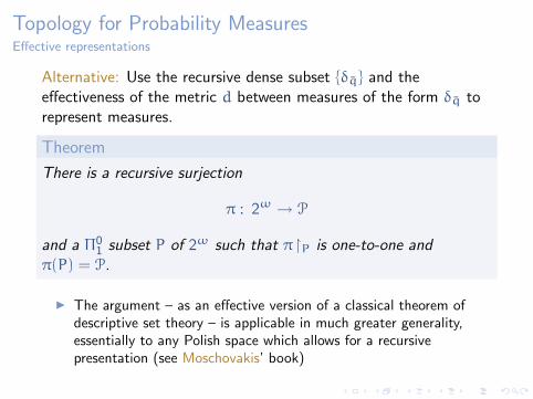
Alternative: Use the recursive dense subset {δq} and theeffectiveness of the metric d between measures of the form δq torepresent measures.

Theorem

There is a recursive surjection

π : 2ω → P

and a Π01 subset P of 2ω such that π�P is one-to-one and

π(P) = P.

I The argument – as an effective version of a classical theorem ofdescriptive set theory – is applicable in much greater generality,essentially to any Polish space which allows for a recursivepresentation (see Moschovakis’ book)

Effectively Closed Sets of MeasuresUniform tests for randomness

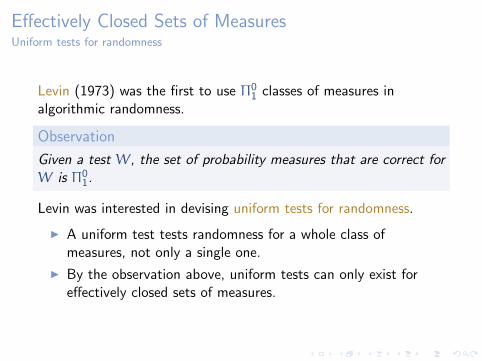
Levin (1973) was the first to use Π01 classes of measures in

algorithmic randomness.

Observation

Given a test W, the set of probability measures that are correct forW is Π0

1.

Levin was interested in devising uniform tests for randomness.

I A uniform test tests randomness for a whole class ofmeasures, not only a single one.

I By the observation above, uniform tests can only exist foreffectively closed sets of measures.

Effectively Closed Sets of MeasuresUniform tests for randomness

Theorem (Levin, 1973)

Given a Π01 class S of probability measures, there exists a test U

such that for any x that passes U there exists a measure µ ∈ S

such that x passes any µ-test.

Note that this is a kind of lowness property.

Hausdorff MeasuresOuter measures from premeasures – Method II

Let ρ(σ) = 2−|σ|s. In general, µρ is not a Borel measure.

I For example, µρ is not additive on cylinders.

Therefore, one refines the transition from a premeasure to an outermeasure.

I Given δ > 0, define the set function

Hhδ (A) = inf

{ ∞∑i=0

ρh(Nσ) : A ⊆⋃i

N(σi), 2−|σi| < δ

}.

I Let Hh(A) = limδ→0 Hhδ (A).

Hausdorff MeasuresDifficulties of Hausdorff measures

The s-dimensional Hausdorff measure Hs is a Borel measure.

I For s = 1, H1 is the same as Lebesgue measure on 2ω.

I For s < 1, all basic open sets have infinite Hs-measure. Inparticular, not all compact subsets of 2ω have finite Hs

measure.

This makes the study of non-integral Hausdorff measures rathercomplicated.

I In particular, if dimH A = s and Hs(A) = ∞.

I Recall: dimH A = inf{s : Hs(A) = 0}.

Mass DistributionsApproximating Hausdorff measure by probability measures

Idea: If a set A supports a probability measure that is “close” touniform, then its Hausdorff dimension is close to 1.

I Recall: The support of a measure µ, supp(µ), is the smallestclosed set F such that µ(2ω \ F) = 0.

I A supports a measure µ if supp(µ) ⊆ A.

Mass Distribution Principle

If A supports a probability measure µ such that for almost all σ,

µ(σ) 6 c2−|σ|s,

then Hs(A) > 1/c.

Mass Distributions and Hausdorff MeasuresFrostman’s Lemma

A fundamental result due to Frostman (1935) asserts that theconverse holds, too, as long as A is not too complex.

Theorem

If A is analytic and dimH A > s > 0, then there exists a probabilitymeasure µ such that supp(µ) ⊆ A and for some c > 0,

µ(σ) 6 c2−|σ|s

Frostman’s Lemma is an important ingredient in the proof thatevery analytic set of inifinite Hs-measure has a subset of finiteHs-measure.

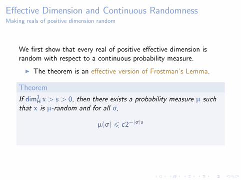
Effective Dimension and Continuous RandomnessMaking reals of positive dimension random

We first show that every real of positive effective dimension israndom with respect to a continuous probability measure.

I The theorem is an effective version of Frostman’s Lemma.

Theorem

If dim1H x > s > 0, then there exists a probability measure µ such

that x is µ-random and for all σ,

µ(σ) 6 c2−|σ|s

Effective Dimension and Continuous RandomnessTransforming Randomness

By the Kucera-Gacs Theorem, there exists a λ-random real y suchthat y >wtt x via some reduction Φ.

I We will use y and the reduction to transform randomness.

I If ν is a probability measure and f : 2ω → 2ω is continuous,then the image measure νf, defined by νf(σ) = ν(f−1[Nσ]),is also a probability measure.

I If f is effective (i.e. truth-table), then f transforms acomputable probability measure into a computable probabilitymeasure.

I Conservation of randomness: If z is ν-random and f istruth-table, then f(z) is νf-random.

Effective Dimension and Continuous RandomnessTransforming Randomness

Problem: The Kucera-Gacs result holds only for a wtt-reduction.

I Nota bene: It can be easily seen that it cannot hold fortruth-table since there are reals which are not random for anycomputable probability measure.

Partial reductions yield semimeasures.

I A (continuous) semimeasure is a function M : 2<ω → [0, 1]

such that M(∅) 6 1 and M(σ) > M(σ _0) + M(σ _1).

Effective Dimension and Continuous RandomnessCompleting semimeasures

We want to define µ(σ), σ ∈ 2<ω. We have to satisfy tworequirements:

1. The measure µ will dominate an image measure induced byΦ. This will ensure that any Martin-Lof random sequence ismapped by Φ to a µ-random sequence.

2. The measure must respect the upper bound.

To meet these requirements, we restrict the values of µ in thefollowing way:

λ(Φ−1(σ)) 6 µ(σ) 6 c2−|σ|s. (*)

This singles out suitable completions of the semimeasure inducedby Φ.

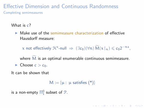
Effective Dimension and Continuous RandomnessCompleting semimeasures

What is c?

I Make use of the semimeasure characterization of effectiveHausdorff measure:

x not effectively Hs-null ⇒ (∃c0)(∀n) M(x�n) 6 c02−ns,

where M is an optimal enumerable continuous semimeasure.

I Choose c > c0.

It can be shown that

M := {µ : µ satisfies (*)}

is a non-empty Π01 subset of P.

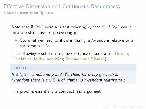
Effective Dimension and Continuous RandomnessA lowness property for Π0

1 classes

Note that if (Vn) were a µ-test covering x, then Φ−1(Vn) wouldbe a λ-test relative to µ covering y.

I So, what we need to show is that y is λ-random relative to µ

for some µ ∈ M.

The following result ensures the existence of such a µ. (Downey,Hirschfeldt, Miller, and Nies; Reimann and Slaman)

Theorem

If B ⊆ 2ω is nonempty and Π01, then, for every y which is

λ-random there is z ∈ B such that y is λ-random relative to z.

The proof is essentially a compactness argument.

Obtaining the Mass DistributionCompact subsets

Frostman’s Lemma yields a mass distribution such thatsupp(µ) ⊆ A.

I The base case is that A is closed.

I The proof for Borel sets uses clever approximations inmeasure.

If A is Π01Π01Π01, then it is Π0

1(z) relative to some z.

I Relativize the argument and add the Π01 conditions for A to

(∗) determining the set of suitable measures M.

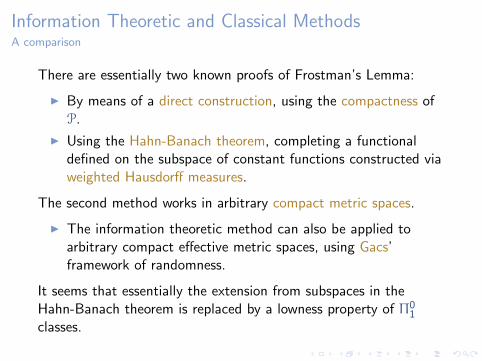
Information Theoretic and Classical MethodsA comparison

There are essentially two known proofs of Frostman’s Lemma:

I By means of a direct construction, using the compactness ofP.

I Using the Hahn-Banach theorem, completing a functionaldefined on the subspace of constant functions constructed viaweighted Hausdorff measures.

The second method works in arbitrary compact metric spaces.

I The information theoretic method can also be applied toarbitrary compact effective metric spaces, using Gacs’framework of randomness.

It seems that essentially the extension from subspaces in theHahn-Banach theorem is replaced by a lowness property of Π0

1

classes.