Effects of Fiscal Shocks in a Globalized World

Alan J. Auerbach University of California, Berkeley

Yuriy Gorodnichenko

University of California, Berkeley

Paper presented at the 15th Jacques Polak Annual Research Conference Hosted by the International Monetary Fund Washington, DC─November 13–14, 2014 The views expressed in this paper are those of the author(s) only, and the presence

of them, or of links to them, on the IMF website does not imply that the IMF, its Executive Board, or its management endorses or shares the views expressed in the paper.

1155TTHH JJAACCQQUUEESS PPOOLLAAKK AANNNNUUAALL RREESSEEAARRCCHH CCOONNFFEERREENNCCEE NNOOVVEEMMBBEERR 1133––1144,, 22001144

1  

This draft: October 29, 2014

 

 

EFFECTS OF FISCAL SHOCKS IN A GLOBALIZED WORLD

Alan J. Auerbach and Yuriy Gorodnichenko University of California, Berkeley and NBER

Abstract: While theoretical models consistently predict that government spending shocks should lead to appreciation of the domestic currency, empirical studies have been stubbornly finding depreciation. Using daily data on U.S. defense spending (announced and actual payments), we document that the dollar immediately and strongly appreciates after announcements about future government spending. In contrast, actual payments lead to no discernable effect on the exchange rate. We examine responses of other variables at the daily frequency and explore how the responses of the exchange rate to fiscal shocks varies over the business cycle as well as at the zero lower bound and in normal times.

JEL codes: E62, F41

Key words: fiscal multiplier, fiscal spillover, exchange rate, high-frequency analysis.

Acknowledgment: We are grateful to Seunghwan Lim, Walker Ray, and Mauricio Ulate for excellent research assistance. We thank Olivier Coibion, Pierre-Olivier Gourinchas, and Johannes Wieland for comments, and Andrew Austin and David Newman for guidance regarding the defense appropriations process. Gorodnichenko thanks the NSF for financial support. Auerbach thanks the Burch Center for Tax Policy and Public Finance for financial support.

2  

I. Introduction

What are the effects of fiscal policy on aggregate economic activity in a globalized world? This

is a key question in current policy and academic debates. The central challenge in this debate is

how to identify fiscal shocks in the data. Previous research has used narrative or structural time

series (SVAR) methods to isolate unanticipated, exogenous innovations to government spending

or revenue. While these approaches have many desirable properties, they typically have been

applied at quarterly or even annual frequencies. These low frequencies can limit the plausibility

of identifying assumptions (e.g., minimum delay restriction for government spending) and

reduce statistical power (e.g., narrative shocks can account for only a few historical changes in

fiscal variables). We address this challenge by using daily data on U.S. government spending.

Using daily variation does limit the scope of our investigation, for we are unable to

measure the effects of shocks on slow moving aggregate variables, like real gross domestic

product (GDP), for which comparable high-frequency data are unavailable. However, high-

frequency analysis greatly enhances our ability to assess reactions of forward-looking variables

such as exchange rates, asset prices, yields, spreads, commodity prices, etc. In previous research,

analyses of how these variables react to government spending or revenue shocks were very

limited because it was hard to rule out reverse causality using low-frequency data. In contrast,

one can be fairly certain that, on a given day, shocks to actual or contracted payments of the U.S.

government are not affected by economic news and hence causation is likely to flow from fiscal

variables to forward-looking variables.

Since the U.S. economy is a dominant force in the world economy, domestic U.S. fiscal

shocks are likely to have tangible effects on the rest of the world. However, the workings of

these effects have been relatively understudied for several reasons. First, the magnitude of fiscal

spillovers is likely to depend heavily on how exchange rates respond to fiscal shocks. However,

as we discussed above, exchange rates are forward-looking variables and therefore it has been

hard to establish causality. Second, typical time series analyses relied on relatively short time

series and thus the scope of variables one could analyze was limited. In contrast, we have

thousands of observations and consequently can examine how fiscal shocks propagate to the rest

of the world through changes in exchange rates vis-à-vis changes in commodity prices or

liquidity spreads. Third, asset prices are likely to move at the time when news about changes in

3  

government spending arrives rather than when the changes actually occur. With low frequency

data, it is difficult to obtain precise timing of news and therefore one is likely to obtain

attenuated responses to changes in government spending because low frequency analysis mixes

the impact reaction to the news with the dynamics after the news. In contrast, using a daily

frequency enables us to time shocks with high precision. Finally, at the daily frequency we can

investigate cyclical variation of the response of exchange rates or other variables to various types

of fiscal shocks. Previous research was greatly constrained in this context because we have only

a handful of low frequency observations when economies are in recession or at the zero lower

bound (ZLB).

We construct two daily series of government spending. The first series is payments to

defense contractors reported in the daily statements of the U.S. Treasury. The second series is the

announced volume of contracts awarded daily by the U.S. Department of Defense. Since one

series measures actual outlays while the other provides a measure of future government

spending, using these two series helps us to underscore the key role of fiscal foresight for timing

shocks to government spending as well as responses to these shocks. While it is possible to

construct more government spending variables at the daily frequency, we focus on military

spending to minimize the possibility of reserve causality and other forms of endogeneity. We

validate our daily military spending series by comparing them to standard government spending

data available at lower frequencies and by relating them to major military developments.

While interpretation of spending shocks at this high frequency may be complex—we

discuss that these shocks may include “level” (how much to spend), “timing” (when to spend),

and “identity” (who receives government funding) components—we document that certain

shocks to government spending have a non-negligible “level” component, which is the

component typically studied with data at quarterly or annual frequencies. Specifically, we show

that announcements about future military spending move the index of stock prices for firms in

the defense industry.

To keep our analysis focused, we concentrate on how the exchange rate reacts to

government spending shocks because these responses have crucial information for both

policymakers and researchers. For example, these responses can inform policymakers about

objects central for design of fiscal policies, such as the size of fiscal multiplier, the degree of

4  

fiscal spillovers, and the potential benefit of coordinating fiscal policies. These responses can

also help researchers to discriminate among competing models of business cycles and to assess

the relative importance of various frictions usually employed to match moments of the data.

Our key finding is that unanticipated shocks to announced military spending, rather than

actual outlays on military programs, lead to an immediate and tangible appreciation of the U.S.

dollar. This finding is broadly consistent with a variety of workhorse models in international

economics and it suggests that fiscal shocks can have considerable spillovers into foreign

economies. At the same time, this finding contrasts sharply with the results reported in previous

studies. Specifically, the earlier work routinely documented that the domestic currency

depreciates in response to government spending shocks, which is hard to square with the

predictions of classic and modern open-economy models. We argue that this difference in results

is likely to arise from the mis-timing of shocks in previous papers and their use of actual

spending rather than news about spending. In short, we find that using daily series can resolve a

long-standing puzzle in international economics.

To investigate the workings of fiscal spillovers further, we examine reactions of some

key macroeconomic variables (commodity prices, stock market returns, liquidity and risk premia,

etc.) available at the daily frequency. We find little support for military spending shocks

influencing global markets via liquidity or uncertainty effects. Although our estimates have

considerable sampling error, the picture painted by the responses is broadly consistent with the

predictions of the mainstream models where government spending shocks operate through the

demand channel.

This paper contributes to several strands of previous work. First, we build on the vast

literature—started by Meese and Rogoff (1983)—trying, for the most part unsuccessfully, to

relate exchange rate movements and domestic fundamentals such as the stance of fiscal and

monetary policies, the state of the business cycle, and the current account deficit. We show that

the relationship could be more apparent at high frequencies where identification and timing of

shocks to fundamentals and responses to such shocks are more clear-cut. Second, we add to the

body of work studying the effects of fiscal shocks on exchange rate movements (e.g., Monacelli

and Perotti 2010, Ilzetzki et al. 2013, Ravn et al. 2012). This literature consistently has found the

puzzling result that government spending shocks lead to depreciation of the domestic currency.

5  

We argue that the puzzle can be resolved with enhanced identification of government spending

shocks. Third, we contribute to the literature on microstructure determination of the exchange

rate (see Lyons 2006 and Vitale 2007 for a survey). Specifically, we document that government

spending shocks could be an additional determinant of exchange rate fluctuations at high

frequencies. Fourth, we contribute to the rapidly growing strand of the literature focused on

variation in the responses of macroeconomic variables to shocks in different states of the

economy (recession vs. expansion, ZLB vs. non-ZLB). Specifically, we exploit high frequency

variation in fiscal and outcome variables rather than using variation in quarterly or lower

frequencies as in our previous work (e.g., Auerbach and Gorodnichenko 2012a, 2012b, 2013).

Finally, we contribute to the ongoing debate about using actual vs. announced government

spending to identify innovations to fiscal policy (e.g., Ramey 2011, Blanchard and Perotti 2002).

Our results suggest that, in the context of studying responses of asset prices at high frequencies,

one should use announcements about future government spending rather than actual outlays.

We structure the rest of the paper as follows. In the next section, we describe the sources

of daily data on government spending on defense (announcements and actual outlays). In this

section, we also relate the constructed series to alternative sources of information about

government spending to validate our series. Section III presents our econometric framework to

study effects of fiscal shocks. Section IV discusses interpretation of shocks. Section V

documents responses of the exchange rate and other macroeconomic variables to spending

shocks. We also investigate how these responses vary over time and across states of the economy

(e.g., recession vs. expansion; binding zero lower bound on nominal interest rates vs. normal

times). Section VI presents concluding remarks.

II. Data

We use two sources of daily data on U.S. government spending. The first source is the Daily

Statements of the U.S. Treasury. The second source is the daily postings of the Department of

Defense (hereafter DoD) about awarded contracts. In this section, we describe these sources and

discuss pros and cons of each for measuring fiscal shocks.

6  

A. DailyU.S.TreasuryStatements

Since 1993, the U.S. Treasury has published daily reports on the federal government’s actual

receipts and spending. These statements include detailed information by types of receipts and

spending. For example, we know how much money is transferred to defense contractors, to

businesses and individuals as tax rebates, to the unemployed, and to banks (e.g., TARP).

While daily statements offer rich information about outlays of the government, we focus

on payments to defense contractors for several reasons. First, as discussed in Ramey and Shapiro

(1998) and elsewhere, defense spending is less likely than other types of spending to be

determined by current economic conditions. Consistent with this logic, we do not observe any

tangible cyclical variation in the payments on defense contracts. For example, there is barely any

change in the payments over the course of the Great Recession.

Second, payments on defense contracts are much less predictable than other types of

payments at high frequencies. For example, tax rebates have a large seasonal component and

unemployment insurance payments appear to be timed to occur on certain days of the month.

Because we are interested in unanticipated shocks to government spending, using payments on

defense contracts provides a cleaner source of variation.

Third, the Daily Treasury Statements provide limited information on many components

of spending in the early part of the sample, while payments on defense contracts have been

consistently reported in the statements. Thus, we have a long time series for this spending

component. This aspect of the data is important because it allows us to estimate state-dependent

responses of macroeconomic variables to fiscal shocks.

Fourth, defense contracts tend to have a large domestic component. For example,

Schwartz and Ginsberg (2013) estimate that the percentage of DoD contract obligations

performed outside the United States ranged between 6 and 12 percent over the last 15 years or

so. Such concentration on domestic spending helps us rule out large direct spillover (or

“leakage”) effects. That is, one is more likely to obtain a demand spending multiplier with

military contract spending than with other components of government spending that are

associated with a higher fraction of purchases of foreign goods and services.

7  

Finally, defense spending is a major source of variation in government spending and

there is enormous variation in daily payments on defense contracts (Panel A, Figure 1): they vary

from $11 million to $4 billion. The payments aggregated to the monthly frequency are

considerably smoother (Panel B, Figure 1), but even this aggregated series exhibits sizable

volatility. The standard deviation of monthly changes in seasonally adjusted monthly payments

is $1.7 billion, with the range going from a reduction of $4.0 billion to an increase of $5.0

billion. Given that the mean monthly payment to defense contractors is about $20.8 billion,

these magnitudes translate into large percent changes.

To assess the quality of the payments data, we aggregate payments to the quarterly

frequency and compare the resulting series with the corresponding data in the National Income

and Product Accounts (NIPA). We construct the NIPA counterpart of the payments as purchases

of intermediate goods and services (net of own-account investment1 and sales to other sectors)

plus gross investment, which is reported in the BEA’s NIPA Table 3.11.5. Some of the

discrepancy between the series can arise due to differences in timing of purchases (accrual vs.

cash transactions) and the treatment of government enterprise expenditures. Although the

definitions of variables are not aligned perfectly, the payment and NIPA spending series track

each other closely and the levels of the variables are very similar, especially after 2000 (Panel C,

Figure 1). Thus, one can interpret the payment series as a daily proxy for the conventional

measures of military spending available at the quarterly frequency.

B. DepartmentofDefensecontracts

Since 1994, nearly every weekday at 5 pm, the DoD has announced (on

http://www.defense.gov/contracts/) its new contract awards greater than $6.5 million.2 A typical

announcement specifies the duration of the contract, awarded amount, the name of the winner,

location of contract execution, and additional details about the nature of the contract (e.g., fixed

price, “do not exceed”, “cost plus”, etc.). Each contract is assigned a unique code and is

                                                            1 Own-account investment is measured in current dollars by compensation of general government employees and related expenditures for goods and services and is classified as investment in structures, software, and research and development.

2 The threshold for contracts announced on the DoD website varied over time. For the most part of our sample, the threshold was five million dollars.

8  

summarized by a paragraph in an announcement. The contracts tend to be of multi-year duration.

This is an example of a contract awarded on July 28, 2014:

SAIC, McLean, Virginia, was awarded an $89,526,485 cost-plus-incentive fee, incrementally- funded contract with options, for management and technical support for high performance computing services, capabilities, infrastructure, and technologies. Work will be performed at Wright-Patterson Air Force Base, Ohio; Aberdeen Proving Ground, Maryland; Stennis Space Center, Mississippi; Vicksburg, Mississippi; Kihei, Hawaii; Lorton, Virginia; and McLean, Virginia, with an estimated completion date of July 28, 2019. Bids were solicited via the Internet with four received. Research, development, testing and evaluation fiscal 2013 ($18,230,430) and fiscal 2014 ($5,770,000) funds are being obligated at the time of the award. U.S. Army Corps of Engineers, Huntsville, Alabama, is the contracting activity (W912DY-14-F-0103).

In addition to announcing new contracts, the DoD also makes announcements about

modifications to existing contracts. The modifications can be linked to the initial DoD

commitments using the unique contract code, and so one can construct a measure of the

incremental changes in defense contracts. For example, on April 17, 2012, the DoD initially

awarded $78 million to Electric Boat Corp., a Connecticut subsidiary of General Dynamics, for

“long-lead-time material associated with the fiscal 2014 Virginia class submarine (SSN 792).”

Using the unique contract code (N00024-12-C-2115), we can see that Electric Boat Corp. was

later awarded an additional $307 million on December 28, 2012 for “… additional long-lead-

time material associated with the fiscal 2014 Virginia-class submarine SSN 792 and the initiation

of long-lead-time material for the fiscal 2015 Virginia-class submarines SSN 793 and SSN 794”

and then another $520 million dollars on February 4, 2014 for “… additional long lead time

material associated with the two fiscal 2015 Virginia-class submarines (SSN 794 and SSN 795)

and the two fiscal 2016 Virginia-class submarines (SSN 796 and SSN 797).” On April 28, 2014,

the DoD awarded Electric Boat Corp. with a $17.6 billion contract for construction of 10

Virginia-class submarines from fiscal 2014 to 2018. The evolution of modifications on this

contract is fairly typical among contracts. In all likelihood, additional tranches are likely to be

widely anticipated before the DoD announcements. To avoid mixing anticipated and

unanticipated awards, we use only announcements of new contracts, that is, contracts that appear

for the first time on the DoD website.

9  

One drawback of using these data is that the DoD does not provide them in a format

suitable for statistical analysis. To convert this information into usable form, we have

downloaded web pages with announcements from the DoD archive

(http://www.defense.gov/contracts/archive.aspx) and parsed data from the web pages. To verify

the quality of the information, we use several algorithms of parsing information from the text of

announcements, have at least two people check the consistency of collected data, and randomly

check the validity of information extracted from a sample of web pages by independent research

assistants. Overall, the quality of the data appears to be high.

While the announcements are not immediately translated into actual disbursements, using

announcements offers one key potential advantage. Standard theory predicts that unconstrained,

forward-looking agents should react at the time of the news rather than when actual spending

occurs. The announcements can thus provide a better timing for spending shocks, as measured by

the present value of contract awards.

Similar to daily spending on defense contracts reported by the U.S. Treasury, daily totals

of announced contracts show huge variation (Panel A, Figure 2). The awarded amounts vary

from $3 million to almost $25 billion with a standard deviation of $1.2 billion and a mean of

$450 million. The daily totals of awarded contracts are weakly (0.08) correlated with daily

spending on defense contracts.

In contrast to daily payments, daily contract awards do not appear much smoother when

aggregated to monthly frequency (Panel B, Figure 2). The time series of monthly totals of

awarded contracts is characterized by low serial correlation and spikes without any discernible

seasonal pattern. Furthermore, these spikes in monthly totals can be related to major military

developments. For example, we observe a surge in awarded contracts immediately after the 9/11

terrorist attack, the start of the second Iraq war in 2003, the Russo-Georgian war in 2008, and the

start of Operation New Dawn (a major counter-insurgency operation in Iraq). In contrast, we

observe no significant movements in actual payments on defense contracts.

C. Seasonalvariationandotherpredictablecomponents

While daily Treasury or DoD data provide considerable variation, their use presents a challenge.

Specifically, economic theory predicts unanticipated movements in actual and promised

10  

spending should have stronger effects than anticipated ones. However, the daily data series can

have predictable movements, for example because of institutional constraints such as budget

cycles in military contract awards or spending disbursements. In particular, the daily data exhibit

predictable movements on certain days of the week, days/weeks of the month, and months of the

year, so one may observe systematic cycles at a variety of frequencies.

Unfortunately, there is no benchmark method for purging seasonal components from

daily data. Popular approaches such as the X-12 algorithm are not available at a daily frequency.

Using an extended set of dummy variables to capture seasonal effects could be unproductive

because it would require many parameters to be estimated and run the risk of overfitting. To

address this challenge, we use a novel framework developed in De Livera, Hyndman, and Snyder

(2011). This framework allows for trends and multiple seasonal components modeled as a

parsimonious series of trigonometric functions. After extensive specification searches, we

include four cycles with periods that correspond to weekly, fortnightly, monthly, and yearly

durations. In our analysis, we use military spending data deseasonalized and detrended using this

approach. Appendix Table 1 presents descriptive statistics for the constructed government

spending series.

III. Econometricframework

In our baseline specification, we follow our earlier work (Auerbach and Gorodnichenko 2012a,

2013) and estimate the effect of government spending using direct projections as in Jorda (2005).

Specifically, we construct impulse responses by running a series of regressions:

∑ Δ ∑ Δ

, 0, … , (1)

where Δ is the first difference operator and the impulse response for an outcome variable is

given by . As we discuss in Auerbach and Gorodnichenko (2012a), this approach has a

number of advantages. For example, in contrast to low-order vector autoregressions (VARs), it

11  

does not constrain the shape of the impulse response function (IRF).3 This property of direct

projection may be important in the context of volatile daily series with complex serial correlation

structure. Furthermore, this approach allows straightforward estimation of state-dependent

responses. Finally, note that when we construct the response of to a change in , the

contemporaneous variation of is purified from movements predictable by lags of and .4

This specification also corresponds to the standard VAR approach (e.g., Blanchard and

Perotti 2002) where government spending is ordered first in the Cholesky decomposition. This

ordering reflects the identifying assumption that a measure of government spending does not

respond contemporaneously to innovations in . Given that we work with at daily frequency,

this assumption is likely to be satisfied.

We extend the direct-projections approach to allow the responses to vary by the state of

the economy. For example for the case where regimes correspond to recessions and expansions,

we estimate specifications of the following type:

∑ Δ ∑ Δ

∑ Δ ∑ Δ

, 0,… , (2)

where and are indicator or probability variables measuring

the state of the economy. The impulse responses for the recession and expansion regimes are

given by and respectively. As we discuss in our earlier work, the direct-

projections approach to estimating state-dependent effects has a number of advantages over

estimating such effects in a standard VAR framework, which we did in Auerbach and

Gorodnichenko (2012b). For example, it automatically incorporates the effect of government

                                                            3 In contrast to vector autoregressions, the error term in specification (1) and other similar specifications is potentially serially correlated for 1 and therefore one has to use Newey-West or similar estimators to calculate standard errors correctly.

4 In Auerbach and Gorodnichenko (2012a,b, 2013), we use professional forecasts to further purify government spending series of predictable movements. Such forecasts unfortunately are not available at a daily frequency. We use twenty lags in all specifications; that is, 20.

12  

spending shocks on the state itself. Furthermore, the approach can be extended to estimation

based on more sophisticated classifications of regimes, such as recession with a binding zero

lower bound (ZLB) on short-term nominal interest rates:

,

,

, 1

, 1

∑ , Δ

∑ , Δ

∑ , Δ 1

∑ , Δ 1

, 0,… , (3)

where is a dummy variable equal to one when the economy is at the ZLB and zero

otherwise. If one is interested in impulse responses of variable to a shock in variable in

recession with a binding ZLB, the impulse response is given by , .

IV. Interpretationofinnovationsingovernmentspending

Conventional macroeconomic analyses of how government spending affects the economy

routinely use innovations to government spending as shocks. At relatively low frequencies (e.g.,

quarterly or annual), this treatment of innovations may be a reasonable approach as the

frequency at which innovations are measured roughly corresponds to the frequency of

government spending decisions. The interpretation of changes in government spending is more

complex at higher frequencies.

For example, the day-to-day variation in amounts of government spending could have

little bearing on total spending over a longer period such as a quarter or a year, perhaps capturing

13  

allocation of resources over time (i.e., news about timing of spending, or “timing news”) rather

than decisions about the level of resources committed for spending (i.e., news about levels of

spending, or “level news”). Economic theory predicts that timing news should be considerably

less powerful than level news. However, previous research (e.g., Parker et al. 2013) has found

that even news about timing can affect economic activity. If variation in daily spending is

dominated by timing news, one may expect that our estimates are likely to be a lower bound for

the responses to news about levels.

In the context of DoD announcements, there could be additional uncertainty about the

identity of firms that receive a contract but little or no uncertainty about the magnitude of the

contract (i.e., “identity news”). For example, the public may know that the DoD plans to award a

$10 billion contract to build a new fleet of bombers and the only uncertainty from the perspective

of the public is the identity of the contract winner, e.g., Boeing or Lockheed. In this case,

specific DoD contract awards may resolve no uncertainty at the aggregate level. If DoD

announcements are dominated by such identity news, one may find weak, if any, reaction of

macroeconomic variables to DoD announcements.

The plausibility that DoD announcement might provide “level news” is increased by the

flexibility of the government spending process with respect to defense. Like other government

spending programs, defense spending proceeds through a process beginning with the submission

of the President’s budget and continuing through the Congressional appropriations process,

which creates budget authority for committing the funds that are allocated by the contracts in our

DoD announcement data. However, the funds allocated in any particular contract announcement

do not necessarily come from current-year authorizations. First, through the procedure of

“multiyear procurement,”5 the DoD can award contracts for which future-year expenditures will

be funded through future-year budget authority, rather than current-year authority. Such

procurement requires Congressional approval and may involve penalties if subsequent funding is

not provided, and so may provide news about the level of expected future appropriations.

Second, as the July 28, 2014 announcement from our sample given above indicates, budget

authority may be carried over from one fiscal year to the next. Unobligated budget authority can

                                                            5 For details, see the discussion in O’Rourke and Schwartz (2014).

14  

be carried over for one or more fiscal years if the appropriations measure specified a “no-year”

or multi-year period of availability6, which is common in DoD accounts. Thus, the present value

of spending from a particular year’s budget is affected by when funds in that budget are actually

committed.

To assess the importance of level news in the daily payments and daily contract

announcements data, we use specification (1) with the stock price index of firms in the defense

industry as the dependent variable. If the only source of variation in DoD announcements is

identity news, then stock prices of individual corporations may react to the news but one should

not observe a reaction in the index since a win for Boeing is a loss for Lockheed. If the only

source of variation in payments or contract announcements is timing news, then the index should

not react to actual payments or announcements because that information should already be

incorporated in the stock prices. If the index reacts to daily variation in payments or

announcements, one can have more confidence that level news is an important source of

variation in these series. Indeed, Fisher and Peters (2010) document that movements in the index

of stock prices of major defense contractors have a significant predictive power for future

military spending.

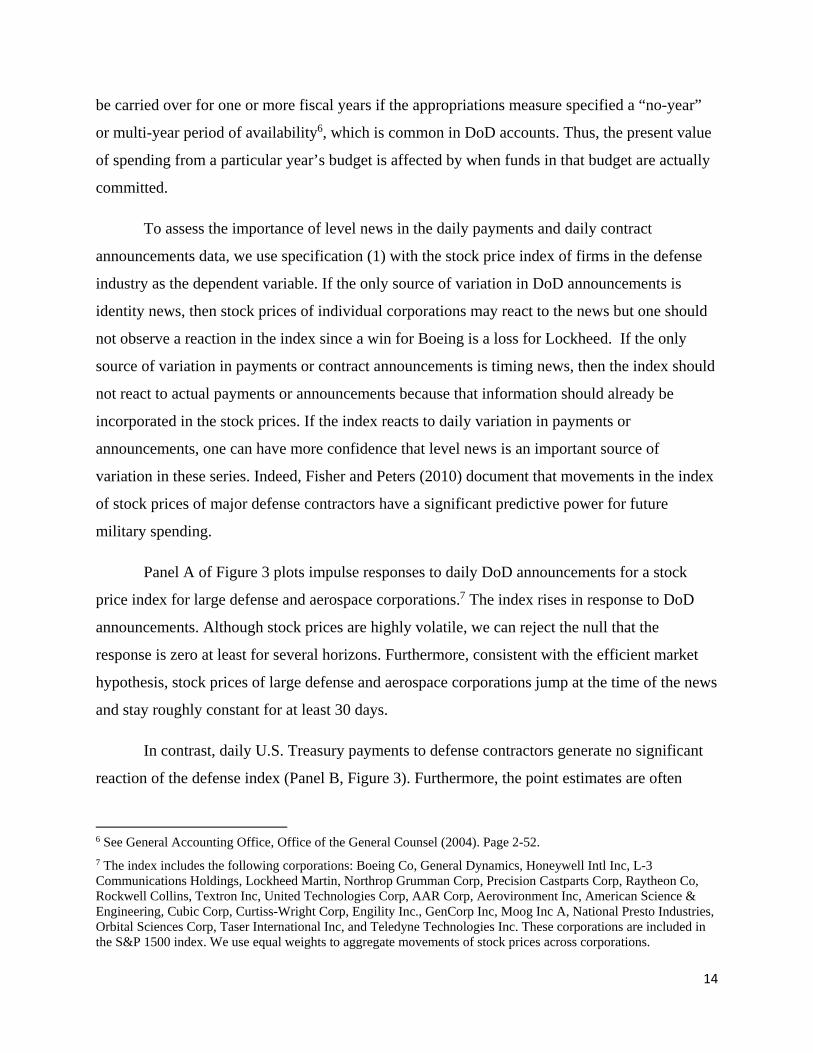
Panel A of Figure 3 plots impulse responses to daily DoD announcements for a stock

price index for large defense and aerospace corporations.7 The index rises in response to DoD

announcements. Although stock prices are highly volatile, we can reject the null that the

response is zero at least for several horizons. Furthermore, consistent with the efficient market

hypothesis, stock prices of large defense and aerospace corporations jump at the time of the news

and stay roughly constant for at least 30 days.

In contrast, daily U.S. Treasury payments to defense contractors generate no significant

reaction of the defense index (Panel B, Figure 3). Furthermore, the point estimates are often

                                                            6 See General Accounting Office, Office of the General Counsel (2004). Page 2-52.

7 The index includes the following corporations: Boeing Co, General Dynamics, Honeywell Intl Inc, L-3 Communications Holdings, Lockheed Martin, Northrop Grumman Corp, Precision Castparts Corp, Raytheon Co, Rockwell Collins, Textron Inc, United Technologies Corp, AAR Corp, Aerovironment Inc, American Science & Engineering, Cubic Corp, Curtiss-Wright Corp, Engility Inc., GenCorp Inc, Moog Inc A, National Presto Industries, Orbital Sciences Corp, Taser International Inc, and Teledyne Technologies Inc. These corporations are included in the S&P 1500 index. We use equal weights to aggregate movements of stock prices across corporations.

15  

negative so that overall effects are small not only statistically but also economically. These

impulse responses are consistent with the view that timing shocks dominate level shocks in daily

payments. In this case, one may expect weaker reactions of macroeconomic variables to shocks

in daily payments than to shocks in contract announcements.

V. Results

In an ideal setting, one would like to study responses of many macroeconomic variables at high

frequencies to understand the effects and transmission mechanisms of government spending

shocks. Unfortunately, most macroeconomic variables relevant for our analysis (e.g., imports and

exports) are available only at a monthly or quarterly frequency, and even if available might react

too slowly for one to observe an immediate response in daily data. As a result, our analysis

focuses on asset prices available at a daily frequency. While we study the effects of government

spending on various asset prices, we emphasize the dynamics of the exchange rate response

because they represent a key channel for many proposed transmission mechanisms.

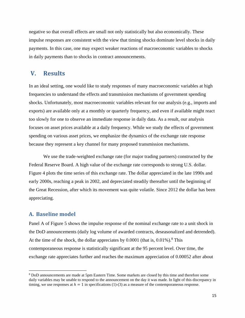
We use the trade-weighted exchange rate (for major trading partners) constructed by the

Federal Reserve Board. A high value of the exchange rate corresponds to strong U.S. dollar.

Figure 4 plots the time series of this exchange rate. The dollar appreciated in the late 1990s and

early 2000s, reaching a peak in 2002, and depreciated steadily thereafter until the beginning of

the Great Recession, after which its movement was quite volatile. Since 2012 the dollar has been

appreciating.

A. Baselinemodel

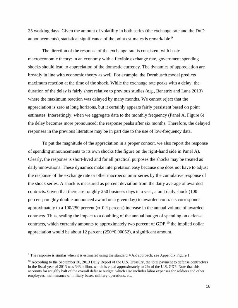
Panel A of Figure 5 shows the impulse response of the nominal exchange rate to a unit shock in

the DoD announcements (daily log volume of awarded contracts, deseasonalized and detrended).

At the time of the shock, the dollar appreciates by 0.0001 (that is, 0.01%).8 This

contemporaneous response is statistically significant at the 95 percent level. Over time, the

exchange rate appreciates further and reaches the maximum appreciation of 0.00052 after about

                                                            8 DoD announcements are made at 5pm Eastern Time. Some markets are closed by this time and therefore some daily variables may be unable to respond to the announcement on the day it was made. In light of this discrepancy in timing, we use responses at 1 in specifications (1)-(3) as a measure of the contemporaneous response.

16  

25 working days. Given the amount of volatility in both series (the exchange rate and the DoD

announcements), statistical significance of the point estimates is remarkable.9

The direction of the response of the exchange rate is consistent with basic

macroeconomic theory: in an economy with a flexible exchange rate, government spending

shocks should lead to appreciation of the domestic currency. The dynamics of appreciation are

broadly in line with economic theory as well. For example, the Dornbusch model predicts

maximum reaction at the time of the shock. While the exchange rate peaks with a delay, the

duration of the delay is fairly short relative to previous studies (e.g., Benetrix and Lane 2013)

where the maximum reaction was delayed by many months. We cannot reject that the

appreciation is zero at long horizons, but it certainly appears fairly persistent based on point

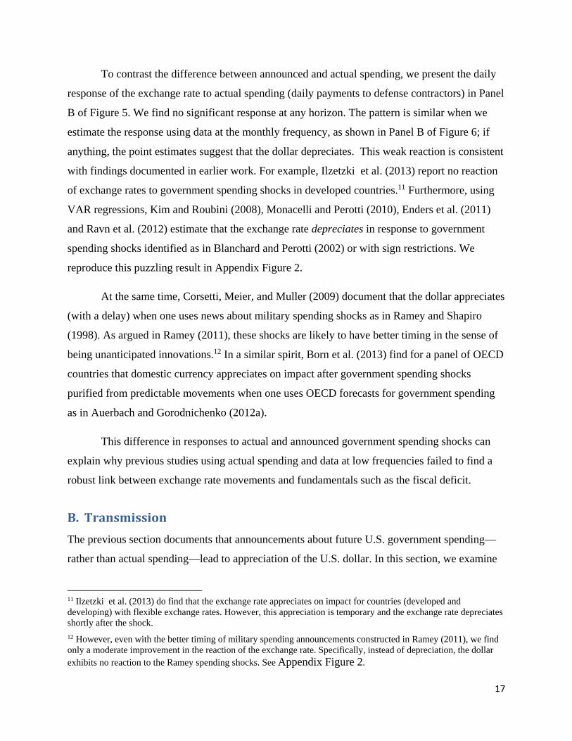
estimates. Interestingly, when we aggregate data to the monthly frequency (Panel A, Figure 6)

the delay becomes more pronounced: the response peaks after six months. Therefore, the delayed

responses in the previous literature may be in part due to the use of low-frequency data.

To put the magnitude of the appreciation in a proper context, we also report the response

of spending announcements to its own shocks (the figure on the right-hand side in Panel A).

Clearly, the response is short-lived and for all practical purposes the shocks may be treated as

daily innovations. These dynamics make interpretation easy because one does not have to adjust

the response of the exchange rate or other macroeconomic series by the cumulative response of

the shock series. A shock is measured as percent deviation from the daily average of awarded

contracts. Given that there are roughly 250 business days in a year, a unit daily shock (100

percent; roughly double announced award on a given day) to awarded contracts corresponds

approximately to a 100/250 percent ( 0.4 percent) increase in the annual volume of awarded

contracts. Thus, scaling the impact to a doubling of the annual budget of spending on defense

contracts, which currently amounts to approximately two percent of GDP,10 the implied dollar

appreciation would be about 12 percent (250*0.00052), a significant amount.

                                                            9 The response is similar when it is estimated using the standard VAR approach; see Appendix Figure 1.

10 According to the September 30, 2013 Daily Report of the U.S. Treasury, the total payment to defense contractors in the fiscal year of 2013 was 343 billion, which is equal approximately to 2% of the U.S. GDP. Note that this accounts for roughly half of the overall defense budget, which also includes labor expenses for soldiers and other employees, maintenance of military bases, military operations, etc.

17  

To contrast the difference between announced and actual spending, we present the daily

response of the exchange rate to actual spending (daily payments to defense contractors) in Panel

B of Figure 5. We find no significant response at any horizon. The pattern is similar when we

estimate the response using data at the monthly frequency, as shown in Panel B of Figure 6; if

anything, the point estimates suggest that the dollar depreciates. This weak reaction is consistent

with findings documented in earlier work. For example, Ilzetzki et al. (2013) report no reaction

of exchange rates to government spending shocks in developed countries.11 Furthermore, using

VAR regressions, Kim and Roubini (2008), Monacelli and Perotti (2010), Enders et al. (2011)

and Ravn et al. (2012) estimate that the exchange rate depreciates in response to government

spending shocks identified as in Blanchard and Perotti (2002) or with sign restrictions. We

reproduce this puzzling result in Appendix Figure 2.

At the same time, Corsetti, Meier, and Muller (2009) document that the dollar appreciates

(with a delay) when one uses news about military spending shocks as in Ramey and Shapiro

(1998). As argued in Ramey (2011), these shocks are likely to have better timing in the sense of

being unanticipated innovations.12 In a similar spirit, Born et al. (2013) find for a panel of OECD

countries that domestic currency appreciates on impact after government spending shocks

purified from predictable movements when one uses OECD forecasts for government spending

as in Auerbach and Gorodnichenko (2012a).

This difference in responses to actual and announced government spending shocks can

explain why previous studies using actual spending and data at low frequencies failed to find a

robust link between exchange rate movements and fundamentals such as the fiscal deficit.

B. Transmission

The previous section documents that announcements about future U.S. government spending—

rather than actual spending—lead to appreciation of the U.S. dollar. In this section, we examine

                                                            11 Ilzetzki et al. (2013) do find that the exchange rate appreciates on impact for countries (developed and developing) with flexible exchange rates. However, this appreciation is temporary and the exchange rate depreciates shortly after the shock.

12 However, even with the better timing of military spending announcements constructed in Ramey (2011), we find only a moderate improvement in the reaction of the exchange rate. Specifically, instead of depreciation, the dollar exhibits no reaction to the Ramey spending shocks. See Appendix Figure 2.

18  

responses of additional macroeconomic variables to have a more complete picture of how

spending shocks are transmitted.

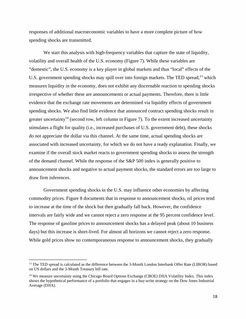
We start this analysis with high-frequency variables that capture the state of liquidity,

volatility and overall health of the U.S. economy (Figure 7). While these variables are

“domestic”, the U.S. economy is a key player in global markets and thus “local” effects of the

U.S. government spending shocks may spill over into foreign markets. The TED spread,13 which

measures liquidity in the economy, does not exhibit any discernable reaction to spending shocks

irrespective of whether these are announcements or actual payments. Therefore, there is little

evidence that the exchange rate movements are determined via liquidity effects of government

spending shocks. We also find little evidence that announced contract spending shocks result in

greater uncertainty14 (second row, left column in Figure 7). To the extent increased uncertainty

stimulates a flight for quality (i.e., increased purchases of U.S. government debt), these shocks

do not appreciate the dollar via this channel. At the same time, actual spending shocks are

associated with increased uncertainty, for which we do not have a ready explanation. Finally, we

examine if the overall stock market reacts to government spending shocks to assess the strength

of the demand channel. While the response of the S&P 500 index is generally positive to

announcement shocks and negative to actual payment shocks, the standard errors are too large to

draw firm inferences.

Government spending shocks in the U.S. may influence other economies by affecting

commodity prices. Figure 8 documents that in response to announcement shocks, oil prices tend

to increase at the time of the shock but then gradually fall back. However, the confidence

intervals are fairly wide and we cannot reject a zero response at the 95 percent confidence level.

The response of gasoline prices to announcement shocks has a delayed peak (about 10 business

days) but this increase is short-lived. For almost all horizons we cannot reject a zero response.

While gold prices show no contemporaneous response to announcement shocks, they gradually

                                                            13 The TED spread is calculated as the difference between the 3-Month London Interbank Offer Rate (LIBOR) based on US dollars and the 3-Month Treasury bill rate.

14 We measure uncertainty using the Chicago Board Options Exchange (CBOE) DJIA Volatility Index. This index shows the hypothetical performance of a portfolio that engages in a buy-write strategy on the Dow Jones Industrial Average (DJIA).

19  

fall and this decline is statistically significant after about 20 business days. Responses to

payment shocks are similar but the contemporaneous reactions to these shocks are attenuated.

Many theoretical models impose a tight link between movements in exchange rates and

interest rates. Typically, appreciation of the U.S. dollar is associated with higher U.S. real

interest rates. To preserve space, we report (Figure 9) only contemporaneous responses ( 1 in

specification (1)) of interest rates and inflation expectations at different maturities so that one can

observe the behavior of the yield curve. Announcement shocks tend to raise short-term (less than

a year) interest rates for U.S. government debt and for interbank loans (LIBOR). The response is

not statistically significant which, apart from sampling uncertainty, may also signal the power of

the Fed to control short-term interest rates. The point estimates for longer rates are close to zero.

In contrast, announcement shocks appear to shift up the whole “yield curve” for inflation

expectations measured from the prices of inflation swaps at different maturities. Unfortunately,

we have measures of inflation expectations only for horizons greater than a year while the

movements in the nominal interest rates are most discernable at much shorter horizons. Thus, we

cannot establish if changes in inflation expectations at these short horizons are sufficiently large

to offset changes in nominal rates. For longer horizons, the responses to announcement shocks

are imprecisely estimated. While our results are statistically inconclusive about the importance of

the real interest rate response, the point estimates of the responses are broadly in line with the

predictions of workhorse models. In contrast, the picture is mixed for responses to payment

shocks (in the right panel of Figure 9). Inflation expectations tend to decrease and nominal rates

for U.S. government debt tend to fall while the nominal rates in the interbank market tend to rise.

It’s hard to reconcile these responses in a standard framework.

Finally, we examine how stock market indices for foreign markets react to U.S.

government spending shocks. We focus on large exchanges with long time series. Specifically,

we study responses of the NIKKEI 225 (Japan), the FTSE 100 (the U.K.) and the TSX (Canada).

Announcement shocks tend to raise these indices although, again, the confidence bands are wide.

We find a statistically significant, positive response only for the FTSE 100 and the TSX shortly

after the shock. In contrast, payment shocks appear to lead to declines in foreign stock market

indices.

20  

Overall, these results suggest spending shocks appear to increase the level of demand in

the global economy. Oil/gasoline prices increase, while the price of gold—a commodity often

used to hedge against recessions—decreases. Domestic interest rates and inflation expectations

rise. Foreign stock markets boom. Alternative explanations based on liquidity and volatility risks

seem to have no clear support. However, sampling uncertainty in the estimated responses is large

and, obviously, such interpretation is tentative at best.

C. Robustness

Given that the period we study (1994-2014) is characterized by dramatic volatility in the

economy and in asset prices (e.g., the Great Recession), we explore in this section whether our

results are driven by particular events or subsamples. As a first pass, we estimate impulse

responses for the pre-Great Recession period, ending in December, 2007. We find that the

patterns estimated on the full sample are similar to those estimated on the pre-crisis period (Panel

A, Figure 11). The response of the exchange rate to a DoD announcement is very similar for

short horizons to those in Figure 5 although there is no upward trend as horizons lengthen. At

the same time, the dollar depreciates (rather than stays at roughly zero) in response to increased

payments to defense contractors.

A binding zero lower bound (ZLB) was a key aspect of the Great Recession; even now,

more than five years since the recession trough, short-term interest rates are at ultra-low levels in

the United States and many other developed countries. Wieland (2012) shows that the response

of the exchange rate to a government spending shock at a binding ZLB can be different from the

response in normal times (i.e., outside the ZLB). Specifically, a government spending shock can,

in theory, lead to depreciation (rather than appreciation) of the exchange rate when the economy

operates at the zero lower bound. Intuitively, in normal times when government spending shocks

increase demand and hence generate inflation, the central bank raises the real interest rate to cool

down the economy. This increase in the real interest rate yields appreciation of the domestic

currency to keep asset markets cleared. In contrast, when the ZLB is binding, the central bank

cannot raise nominal interest rates and therefore inflation generated by increased government

spending translates into a fall in real interest rates. Such reaction of real interest rates at the ZLB

leads to depreciation of the domestic currency. As a result, the fiscal multiplier in an open

economy can be larger than in a closed economy when the ZLB is binding.

21  

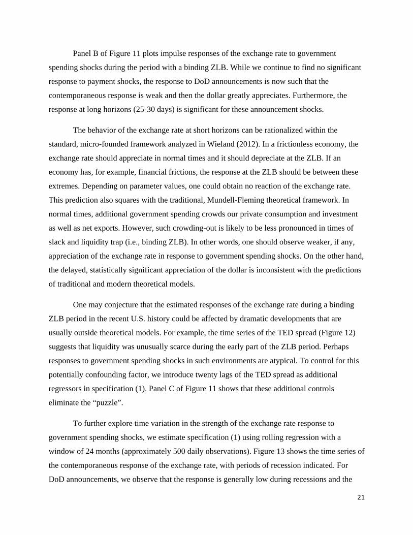
Panel B of Figure 11 plots impulse responses of the exchange rate to government

spending shocks during the period with a binding ZLB. While we continue to find no significant

response to payment shocks, the response to DoD announcements is now such that the

contemporaneous response is weak and then the dollar greatly appreciates. Furthermore, the

response at long horizons (25-30 days) is significant for these announcement shocks.

The behavior of the exchange rate at short horizons can be rationalized within the

standard, micro-founded framework analyzed in Wieland (2012). In a frictionless economy, the

exchange rate should appreciate in normal times and it should depreciate at the ZLB. If an

economy has, for example, financial frictions, the response at the ZLB should be between these

extremes. Depending on parameter values, one could obtain no reaction of the exchange rate.

This prediction also squares with the traditional, Mundell-Fleming theoretical framework. In

normal times, additional government spending crowds our private consumption and investment

as well as net exports. However, such crowding-out is likely to be less pronounced in times of

slack and liquidity trap (i.e., binding ZLB). In other words, one should observe weaker, if any,

appreciation of the exchange rate in response to government spending shocks. On the other hand,

the delayed, statistically significant appreciation of the dollar is inconsistent with the predictions

of traditional and modern theoretical models.

One may conjecture that the estimated responses of the exchange rate during a binding

ZLB period in the recent U.S. history could be affected by dramatic developments that are

usually outside theoretical models. For example, the time series of the TED spread (Figure 12)

suggests that liquidity was unusually scarce during the early part of the ZLB period. Perhaps

responses to government spending shocks in such environments are atypical. To control for this

potentially confounding factor, we introduce twenty lags of the TED spread as additional

regressors in specification (1). Panel C of Figure 11 shows that these additional controls

eliminate the “puzzle”.

To further explore time variation in the strength of the exchange rate response to

government spending shocks, we estimate specification (1) using rolling regression with a

window of 24 months (approximately 500 daily observations). Figure 13 shows the time series of

the contemporaneous response of the exchange rate, with periods of recession indicated. For

DoD announcements, we observe that the response is generally low during recessions and the

22  

strength of the response appears to have declined over time. That is, the contemporaneous

response is larger and statistically significant in the early part of the sample but becomes close to

zero economically and statistically towards the end of our sample, which is consistent with

results reported in Figure 12. Note that we estimate the strongest response in the mid- to late-

1990s, which was the period of a strong expansion of the U.S. economy. Interestingly, the

response to payment shocks (daily statements of the U.S. Treasury) shows the opposite cyclical

variation: the response is larger in recessions than in expansions, although generally not

significant statistically.

D. Microstructureeffects

Previous studies of exchange rate movements at high frequencies emphasize that macroeconomic

news could be powerful determinants of such movements.15 One may be concerned that our

findings are driven by a correlation between such news and innovations to government spending.

To isolate the effect of government spending shocks from other macroeconomic news at high

frequencies, we construct additional controls for macroeconomic news.

Specifically, we use two measures of innovations to monetary policy. The first measure is

the difference between the fed funds rate target announced by the Fed and the expected value of

the rate captured by the futures on the fed funds rate. As in Gorodnichenko and Weber (2013),

we calculate this difference in a tight (30-minute) window around FOMC announcements. The

second measure is the movement in the 5-year Treasury note at the time of the Fed’s

announcements about quantitative easing. Chorodow-Reich (2014, Table 1) reports these

movements in tight windows around the announcements. We use two measures because the first

one is not available at the ZLB while the second was not used by the Fed before the ZLB became

binding.

For other macroeconomic news, we follow Andersen et al. (2003) and calculate the

surprise component in macroeconomic releases as the difference between the released figures

(“realization”) and expectations of money market managers. We construct macroeconomic

surprises for the following variables: GDP, capacity utilization, consumer confidence, CPI core

                                                            15 See Vitale (2007) for a survey.

23  

inflation rate, employment cost index, initial unemployment claims, ISM manufacturing

composite index, index of leading indicators, new home sales, non-farm payrolls, PPI core

inflation rate, retail sales, retail sales excluding motor vehicles, and unemployment.

We use these measures (current values and lags) as additional controls in specification

(1). Figure 14 shows responses of the exchange rate to government spending shocks for different

combinations of the additional controls. By and large, we observe little difference in the

estimated impulse responses relative to what we obtain in the baseline specification, which does

not control for other macroeconomic innovations. This negligible difference in the responses

does not mean that the additional controls have no predictive power for the exchange rate

movements. We find (Appendix Figure 3) that these sources of news do move the exchange rate

significantly. As a result, one can interpret the stability of the responses to government spending

shocks as suggesting little correlation between government spending shocks and the additional

controls.

E. State‐dependentresponses

Results of Section V.C document variation in the responses of the exchange rate to government

spending shocks. In this section, we examine if this variation can be related to the state of

business cycle. We estimate specification (2) with two regimes: recession and expansion as

identified by the National Bureau of Economic Research (NBER). Figure 15 plots the impulse

responses of the nominal exchange rate to DoD announcements (Panel A) and U.S. Treasury

payments to defense contractors (Panel B) for these two regimes. The figure also reports

responses of government spending to its own shocks.

Similar to the previous results, we do not observe any persistence in our measures of

government spending. The response of the exchange rate to announcement shocks in expansion

is also similar to the response we estimate on the full sample in the linear model: the dollar

appreciates on impact and stays appreciated. In contrast, the dollar depreciates to a payment

shock (not statistically significant). Given large standard errors we cannot reject equality of these

responses from the response we obtain in the linear model that pools data across regimes. The

responses to spending shocks in recession, however, are radically different from those in

24  

expansion. The contemporaneous response is weak but, over time, the dollar strongly

appreciates. This pattern applies to announcement and spending shocks.

As we discussed above, the gradual appreciation of the exchange rate is hard to reconcile

in the standard theoretical framework. To assess whether these puzzling dynamics are driven by

a binding ZLB, we estimate specification (3) which provides responses in four regimes:

recession without a binding ZLB (March 2001—November 2001, December 2007—November

2008); recession with a binding ZLB (December 2008—June 2009); expansion with a binding

ZLB (July 2009—present); expansion without a binding ZLB (October 1994—February 2001,

December 2001—November 2007). We also highlighted before the importance of using the TED

spread for understanding dynamics of the variables during the Great Recession. Hence, we report

estimated responses when lags of the TED spread are excluded (Panel A in Figure 16 and Figure

17 for announcement and payment shocks respectively) and when they are included as controls

(Panel B in the figures).

Consider responses to the announcement shocks (right-hand side of Figure 16) when the

ZLB is not binding. We find that in expansion the dollar appreciates and stays strong. The

contemporaneous response in recession is weaker than in expansion but then we observe a

gradual appreciation. Although the magnitude of the appreciation is larger than the magnitude of

the appreciation in expansion, the standard errors are large and we cannot reject equality of

responses. In addition, we cannot reject the null of zero response in recession. Whether we

control for the TED spread or not makes little difference for the estimates when the ZLB is not

binding.

When the ZLB is binding (left-hand side of Figure 16), the response in expansion is small

and not statistically different from zero. We observe this weak response with and without lags of

the TED spread as controls in specification (3). In contrast, the dollar gradually and strongly

appreciates in recession in the baseline specification. These puzzling dynamics vanish when we

control for the lags of the TED spread. In this case, the response is volatile but it is much smaller

in magnitude than in the case without lags of the TED spread. Furthermore, we cannot reject the

null hypothesis that the response is zero once these controls are introduced. This finding is

consistent with Wieland (2012) documenting that the reaction of the exchange rate to inflation

surprises is close to zero.

25  

When we compare “expansion” responses inside and outside the ZLB after controlling

for the TED spread (Panel B, Appendix Figure 4), we observe that the point estimate of the

response is lower when the ZLB binds than when it doesn’t. The pattern is similar for the

“recession” responses. While we cannot reject the null that the responses are the same across

ZLB and non-ZLB periods, the weaker response of the exchange rate when ZLB is binding is

qualitatively consistent with the modern theoretical models predicting a possibility of such

depreciation (see Wieland 2012).

The responses to payment shocks (Figure 17) are puzzling. For example, the dollar

depreciates (appreciates) when economy is in expansion (recession) and ZLB is not binding.

Controlling for lags of the TED spread attenuates these puzzling dynamics, but even these

additional controls cannot resolve the problem completely.

While we find only a weak statistical support for variation in the response of the

exchange rate to fiscal shocks across regimes (recession vs. expansion; ZLB vs. non-ZLB), one

should not infer that the responses are universally stable. Indeed, Woodford (2011) and others

argue that the difference in the responses across regimes depends on the extent to which shocks

spill from one regime into another. Our strongest results are for announcement shocks, but these

shocks indicate spending over multiple years. Since a typical recession lasts for only a few

quarters, it is possible that the differences across regimes are attenuated.

VI. Concludingremarks

How government spending shocks propagate in interconnected economies is a key question with

a number of positive and normative implications. Yet, despite a great deal of attention to this

question, understanding of the strength and channels of the propagation has been elusive. A main

challenge has been the identification unanticipated shocks to government spending when fiscal

foresight is potentially a dominant feature of the data and government spending can respond

endogenously to the state of the economy. The challenge is particularly acute when

investigations involve movements in asset prices, which respond to information very rapidly.

To address this challenge, we construct two daily series of an important component of

U.S. government spending, actual defense outlays and announcements about future defense

26  

spending. At this high frequency, it is unlikely that spending reacts to developments in the

economy and hence one can rule out reverse causality. Shocks to defense spending are much less

cyclical than other components of government spending, which further reduces the possibility of

endogeneity.

We show that, in contrast to actual outlays, announcements about future spending

robustly lead to a significant and immediate appreciation of the U.S. dollar, which suggests

potentially considerable fiscal spillovers. This finding differs sharply from the results reported in

previous studies that find a depreciation of the currency in response to domestic government

spending shocks, which may be interpreted as leading to “beggar-thy-neighbor” effects. We

argue that this discrepancy is likely to arise for two reasons. First, using daily data rather than

monthly, quarterly or annual data allows us to have a much finer precision in the timing of

shocks and responses. Second, previous studies typically use actual outlays while forward-

looking variables such as the exchange rate are likely to move at the time of the announcement.

In addition to documenting this central result, we also try to shed more light on the

propagation mechanisms by studying responses of other variables. While sampling uncertainty in

our estimates is quite high, the patterns of the responses are broadly consistent with the

predictions of classic and modern open-economy models emphasizing the demand channel of

government spending shocks. Finally, we examine how the response of the exchange rate to

defense spending shocks varies with the state of the economy (recession vs. expansion, binding

zero lower bound vs. normal times). Although we observe interesting variation in the responses,

again sampling uncertainty is too large to reach firm conclusions.

Previous analyses documenting depreciation of the exchange rate after domestic

government spending shocks stimulated development of new models to rationalize such

depreciations, which were puzzling for the workhorse open-economy models. Our results

suggest that, perhaps, further progress should be concentrated on improving identification of

government spending shocks to establish solid foundations for subsequent theoretical work. We

highlight potential benefits of using high-frequency data to study effects of fiscal shocks. We

focus on defense spending but information for other types of spending is available for analyses.

For example, daily statements of U.S. Treasury have information for dozens on spending

components. While our results here suggest relatively weak responses to payments rather than

27  

announcements, previous research suggests that other components of government spending, such

as tax rebates and transfer payments, might have a more noticeable impact. We hope that future

work will exploit this wealth of information.

References

Andersen, Torben, Tim Bollerslev, Francis Diebold, and Clara Vega, 2003. “Micro Effects of Macro Announcements: Real-Time Price Discovery in Foreign Exchange,” American Economic Review 93, 38-62.

Auerbach, Alan J., and Yuriy Gorodnichenko, 2012a. "Fiscal Multipliers in Recession and Expansion," in Fiscal Policy after the Financial Crisis, pages 63-98, National Bureau of Economic Research, Inc.

Auerbach, Alan J., and Yuriy Gorodnichenko, 2012b. "Measuring the Output Responses to Fiscal Policy," American Economic Journal: Economic Policy 4(2), 1-27.

Auerbach, Alan J., and Yuriy Gorodnichenko, 2013. "Output Spillovers from Fiscal Policy," American Economic Review, 103(3), 141-46.

Benetrix, Agustin. S., and Philip R. Lane, 2013. "Fiscal Shocks and the Real Exchange Rate," International Journal of Central Banking 9(3), 6-37.

Blanchard, Olivier, and Roberto Perotti, 2002. “An Empirical Characterization of the Dynamic Effects of Changes in Government Spending and Taxes on Output,” Quarterly Journal of Economics 117(4), 1329-1368.

Born, Benjamin, Falko Juessen, and Gernot J. Müller, 2013. "Exchange rate regimes and fiscal multipliers," Journal of Economic Dynamics and Control 37(2), 446-465.

Chodorow-Reich, Gabriel, 2014. “Effects of Unconventional Monetary Policy on Financial Institutions,” forthcoming in Brookings Papers on Economic Activity.

Corsetti , Giancarlo, André Meier, and Gernot J. Müller, 2009. "Fiscal Stimulus with Spending Reversals," IMF Working Papers 09/106, International Monetary Fund.

De Livera, Alysha M., Rob J. Hyndman, and Ralph D. Snyder, 2011. “Forecasting Time Series With Complex Seasonal Patterns Using Exponential Smoothing,” Journal of the American Statistical Association 106(496), 1513-1527.

Enders, Zeno, Gernot J. Müller, and Almuth Scholl , 2011. "How do fiscal and technology shocks affect real exchange rates? New evidence for the United States," Journal of International Economics 83(1), 53-69.

Fisher, Jonas D.M., and Ryan Peters, 2010. “Using Stock Returns to Identify Government Spending Shocks,” Economic Journal 120(544), 414-436.

General Accounting Office, Office of the General Counsel, 2004. Principles of Federal Appropriations Law, 3rd Edition, Volume 1.

Gorodnichenko, Yuriy, and Michael Weber, 2013. “Are Sticky Prices Costly? Evidence From The Stock Market,” NBER Working Paper No. 18860.

28  

Ilzetzki Ethan, Enrique G. Mendoza, and Carlos A. Vegh, 2013. “How Big (Small?) are Fiscal Multipliers?” Journal of Monetary Economics 60(2), 239-254.

Jorda, Oscar, 2005. “Estimation and Inference of Impulse Responses by Local Projections,” American Economic Review 95(1), 161-182.

Kim, Soyoung, and Nouriel Roubini, 2008. "Twin deficit or twin divergence? Fiscal policy, current account, and real exchange rate in the U.S," Journal of International Economics 74(2), 362-383.

Lyons, Richard, 2006. The Microstructure Approach to Exchange Rates. MIT Press. Meese, Richard, and Kenneth Rogoff, 1983. “Empirical Exchange Rate Models of the Seventies:

Do They Fit Out of the Sample?” Journal of International Economics 13, 3-24. Monacelli, Tommaso, and Roberto Perotti, 2010. "Fiscal Policy, the Real Exchange Rate and

Traded Goods," Economic Journal 120(544), 437-461. O’Rourke, Ronald, and Moshe Schwartz, 2014. Multiyear Procurement (MYP) and Block Buy

Contracting in Defense Acquisition: Background and Issues for Congress. Congressional Research Service Report R41909, July 30.

Parker, Jonathan A., Nicholas S. Souleles, David S. Johnson, and Robert McClelland, 2013. "Consumer Spending and the Economic Stimulus Payments of 2008," American Economic Review 103(6), 2530-2553.

Ramey, Valerie, and Matthew D. Shapiro, 1998. “Costly Capital Reallocation and the Effects of Government Spending,” Carnegie-Rochester Conference Series on Public Policy.

Ramey, Valerie, 2011. “Identifying Government Spending Shocks: It's All In The Timing,” Quarterly Journal of Economics 126(1), 1-50.

Ravn, Morten O., Stephanie Schmitt-Grohé, and Martín Uribe, 2012. "Consumption, government spending, and the real exchange rate," Journal of Monetary Economics 59(3), 215-234.

Schwartz, Moshe, and Wendy Ginsberg, 2013. Department of Defense Trends in Overseas Contract Obligations. Congressional Research Service Report R41820, March 1.

Vitale, Paolo, 2007. “A Guided Tour of The Market Microstructure Approach to Exchange Rate Determination,” Journal of Economic Surveys 21, 903-934.

Wieland, Johannes, 2012. Fiscal Multipliers at the Zero Lower Bound: International Theory and Evidence. UCSD manuscript.

Woodford, Michael, 2011. "Simple Analytics of the Government Expenditure Multiplier," American Economic Journal: Macroeconomics vol. 3(1), 1-35.

29  

Figure 1. Daily measures of government spending.

Panel A. Daily Cash Withdrawals from Fed. Res. Acct. for Defense Vendor Payments.

Panel B. Monthly totals

Panel C. Quarterly totals

Sources: Daily Statements of the U.S. Treasury; Department of Defense, http://www.defense.gov/contracts/archive.aspx. Monthly and quarterly totals are seasonally adjusted.

010

0020

0030

0040

00D

efe

nse

Ven

dor

Pa

ymen

ts,

Mil

$

01jan1995 01jan2000 01jan2005 01jan2010 01jan2015

010

000

2000

030

000

4000

0M

il $

01jan1995 01jan2000 01jan2005 01jan2010 01jan2015

2040

6080

100

120

Bill

ion

$

01jan1995 01jan2000 01jan2005 01jan2010 01jan2015

Defense Vendor Payments, quarterly totalNIPA Defense: Intermed. goods&serv. purchased + Gross Invest.

30  

Figure 2. New contracts awarded by the Department of Defense, millions of dollars.

Panel A. Daily totals

Panel B. Monthly totals

Source: Department of Defense, http://www.defense.gov/contracts/archive.aspx.

050

0010

000

1500

020

000

2500

0C

ont

ract

s aw

ard

ed b

y D

oD

, da

ily to

tal,

Mil

$

01jan1995 01jan2000 01jan2005 01jan2010 01jan2015

9/11

Iraq II

Russo-Georgian

war

OperationNewDawn

010

000

2000

030

000

4000

050

000

Mil

$

01jan1995 01jan2000 01jan2005 01jan2010 01jan2015

New contracts awarded by DoD, monthly totalDefense Vendor Payments, monthly total

31  

Figure 3. Response of index of stock prices of defense corporations to a government spending shock

Panel A. Responses to DoD announcements

Panel B. Responses to a shock in daily payments to defense contractors (U.S. Treasury daily statements)

Notes: Each panel plots impulse responses estimated using specification (1). The dependent variable is the change in the value of price index for stock of defense corporations. The horizon (horizontal axis) is measured in days.

-.00

050

.00

05.0

01

0 10 20 30horizon

IRF 95% confidence interval

Defense and Aerospace index

-.00

4-.

002

0.0

02

.00

4

0 10 20 30horizon

IRF 95% confidence interval

Defense and Aerospace index

32  

Figure 4. Trade Weighted U.S. Dollar Index: Major Currencies

Source: Board of Governors of the Federal Reserve System, H.10 Foreign Exchange Rates.

7080

9010

011

0T

rad

e W

eig

hted

U.S

. Dol

lar

Ind

ex: M

ajo

r C

urre

ncie

s

01jan1995 01jan2000 01jan2005 01jan2010 01jan2015

33  

Figure 5. Impulse responses to a government spending shock, daily data.

Panel A. Department of Defense announcements

Panel B. Daily payments to defense contractors

Notes: Figures show impulse response functions for the Trade Weighted U.S. Dollar Index (Major Currencies) and government spending to a unit shock to government spending. Impulse responses are estimated using specification (1). The horizon (horizontal axis) is measured in days.

0.0

005

.00

1ex

chan

ge r

ate

res

pon

se

0 10 20 30horizon

IRF 95% confidence interval

0.2

.4.6

.81

gove

rnm

ent s

pen

din

g re

spon

se

0 10 20 30horizon

IRF 95% confidence interval

-.00

4-.

002

0.0

02

.00

4ex

chan

ge r

ate

res

pon

se

0 10 20 30horizon

IRF 95% confidence interval

0.5

1go

vern

men

t sp

endi

ng

resp

onse

0 10 20 30horizon

IRF 95% confidence interval

34  

Figure 6. Impulse response to a government spending shock, monthly data.

Panel A. Department of Defense announcements 

Panel B. Daily payments to defense contractors

Notes: Figures show impulse response functions for the Trade Weighted U.S. Dollar Index (Major Currencies) and government spending to a unit shock to government spending. Impulse responses are estimated using specification (1). Daily data are aggregate to monthly frequency. The horizon (horizontal axis) is measured in months.

-.00

10

.00

1.0

02

exch

ange

ra

te r

esp

onse

0 1 2 3 4 5 6 7 8 9 10 11 12horizon (month)

IRF 95% confidence interval

-.5

0.5

1go

vern

men

t sp

endi

ng

resp

onse

0 1 2 3 4 5 6 7 8 9 10 11 12horizon

IRF 95% confidence interval

-.00

001-

5.0

0e-0

60

5.0

0e-0

6.0

000

1.0

000

15ex

chan

ge r

ate

res

pon

se

0 1 2 3 4 5 6 7 8 9 10 11 12horizon (months)

IRF 95% confidence interval

-.5

0.5

1go

vern

men

t sp

endi

ng

resp

onse

0 1 2 3 4 5 6 7 8 9 10 11 12horizon (months)

IRF 95% confidence interval

35  

Figure 7. Responses of additional macroeconomic variables to a government spending shock.

DoD announcements Daily payments

Notes: Impulse responses are estimated using specification (1). All series are taken from FRED© database. FRED codes are reported in parentheses: TED spread (TEDRATE), CBOE DJIA Volatility Index (VXDCLS), S&P500 Stock Price Index (SP500). The horizon (horizontal axis) is measured in days.

-.01

-.00

50

.00

5

0 10 20 30horizon

IRF 95% confidence interval

TED Spread

-.04

-.02

0.0

2.0

4.0

6

0 10 20 30horizon

IRF 95% confidence interval

TED Spread

-.2

-.1

0.1

.2

0 10 20 30horizon

IRF 95% confidence interval

CBOE DJIA Volatility Index

-.5

0.5

11.

5

0 10 20 30horizon

IRF 95% confidence interval

CBOE DJIA Volatility Index

-.00

2-.

001

0.0

01

.00

2

0 10 20 30horizon

IRF 95% confidence interval

S&P 500 Stock Price Index

-.01

-.00

50

.00

5

0 10 20 30horizon

IRF 95% confidence interval

S&P 500 Stock Price Index

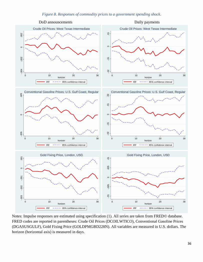
36  

Figure 8. Responses of commodity prices to a government spending shock.

DoD announcements Daily payments

Notes: Impulse responses are estimated using specification (1). All series are taken from FRED© database. FRED codes are reported in parentheses: Crude Oil Prices (DCOILWTICO), Conventional Gasoline Prices (DGASUSGULF), Gold Fixing Price (GOLDPMGBD228N). All variables are measured in U.S. dollars. The horizon (horizontal axis) is measured in days.

-.00

4-.

002

0.0

02

0 10 20 30horizon

IRF 95% confidence interval

Crude Oil Prices: West Texas Intermediate

-.02

-.01

0.0

1

0 10 20 30horizon

IRF 95% confidence interval

Crude Oil Prices: West Texas Intermediate

-.00

50

.00

5

0 10 20 30horizon

IRF 95% confidence interval

Conventional Gasoline Prices: U.S. Gulf Coast, Regular

-.02

-.01

0.0

1.0

2

0 10 20 30horizon

IRF 95% confidence interval

Conventional Gasoline Prices: U.S. Gulf Coast, Regular

-.00

3-.

002

-.00

10

.00

1

0 10 20 30horizon

IRF 95% confidence interval

Gold Fixing Price, London, USD

-.01

-.00

50

.00

5.0

1

0 10 20 30horizon

IRF 95% confidence interval

Gold Fixing Price, London, USD

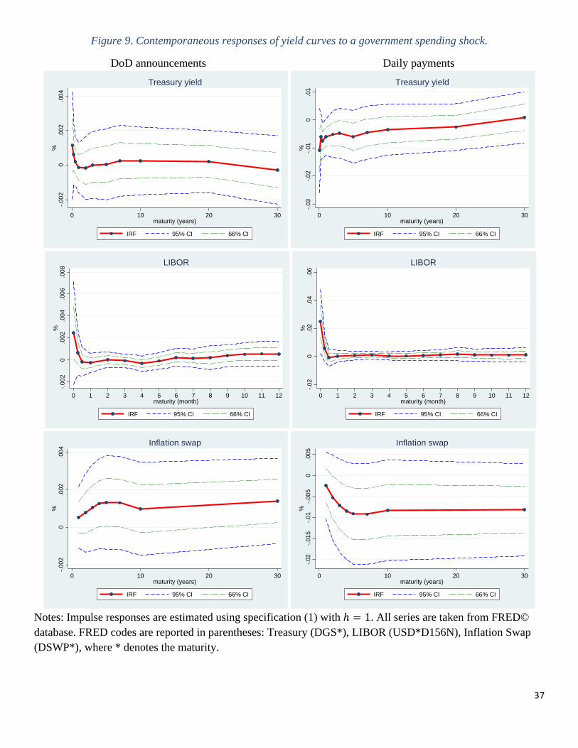
37  

Figure 9. Contemporaneous responses of yield curves to a government spending shock.

DoD announcements Daily payments

Notes: Impulse responses are estimated using specification (1) with 1. All series are taken from FRED© database. FRED codes are reported in parentheses: Treasury (DGS*), LIBOR (USD*D156N), Inflation Swap (DSWP*), where * denotes the maturity.

-.00

20

.00

2.0

04

%

0 10 20 30maturity (years)

IRF 95% CI 66% CI

Treasury yield

-.03

-.02

-.01

0.0

1%

0 10 20 30maturity (years)

IRF 95% CI 66% CI

Treasury yield

-.00

20

.00

2.0

04

.00

6.0

08

%

0 1 2 3 4 5 6 7 8 9 10 11 12maturity (month)

IRF 95% CI 66% CI

LIBOR

-.02

0.0

2.0

4.0

6%

0 1 2 3 4 5 6 7 8 9 10 11 12maturity (month)

IRF 95% CI 66% CI

LIBOR

-.00

20

.00

2.0

04

%

0 10 20 30maturity (years)

IRF 95% CI 66% CI

Inflation swap

-.02

-.01

5-.

01-.

005

0.0

05

%

0 10 20 30maturity (years)

IRF 95% CI 66% CI

Inflation swap

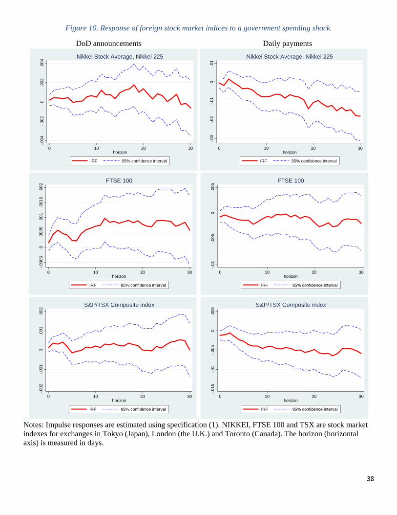
38  

Figure 10. Response of foreign stock market indices to a government spending shock.

DoD announcements Daily payments

Notes: Impulse responses are estimated using specification (1). NIKKEI, FTSE 100 and TSX are stock market indexes for exchanges in Tokyo (Japan), London (the U.K.) and Toronto (Canada). The horizon (horizontal axis) is measured in days.

-.00

4-.

002

0.0

02

.00

4

0 10 20 30horizon

IRF 95% confidence interval

Nikkei Stock Average, Nikkei 225

-.03

-.02

-.01

0.0

1

0 10 20 30horizon

IRF 95% confidence interval

Nikkei Stock Average, Nikkei 225

-.00

050

.00

05.0

01

.00

15.0

02

0 10 20 30horizon

IRF 95% confidence interval

FTSE 100

-.01

-.00

50

.00

5

0 10 20 30horizon

IRF 95% confidence interval

FTSE 100

-.00

2-.

001

0.0

01

.00

2

0 10 20 30horizon

IRF 95% confidence interval

S&P/TSX Composite index

-.01

5-.

01-.

005

0.0

05

0 10 20 30horizon

IRF 95% confidence interval

S&P/TSX Composite index

39  

Figure 11. Stability of the responses to a government spending shock. Panel A. Pre-Great Recession period

Panel B. Period with the binding zero lower bound on the nominal interest rates

Panel C. Period with the binding zero lower bound on the nominal interest rates, control for TED spread.

Notes: Impulse responses are estimated using specification (1). Specification in Panel C also include 20 lags of the TED spread. The horizon (horizontal axis) is measured in days.

-.00

050

.00

05.0

01

exch

ange

ra

te r

esp

onse

0 10 20 30horizon

IRF 95% confidence interval

DoD announcements

-.00

4-.

002

0.0

02

exch

ange

ra

te r

esp

onse

0 10 20 30horizon

IRF 95% confidence interval

Payments to defense contractors

-.00

050

.00

05.0

01

.00

15.0

02

exch

ange

ra

te r

esp

onse

0 10 20 30horizon

IRF 95% confidence interval

DoD announcements

-.00

50

.00

5ex

chan

ge r

ate

res

pon

se

0 10 20 30horizon

IRF 95% confidence interval

Payments to defense contractors

-.00

10

.00

1.0

02

exch

ange

ra

te r

esp

onse

0 10 20 30horizon

IRF 95% confidence interval

DoD announcements

-.00

50

.00

5.0

1ex

chan

ge r

ate

res

pon

se

0 10 20 30horizon

IRF 95% confidence interval

Payments to defense contractors

40  

Figure 12. TED Spread.

Notes: TED spread is calculated as the spread between 3-Month LIBOR based on US dollars and 3-Month Treasury bill.

0.0

01.

00

2.0

03.

00

4.0

05.

00

TE

D S

pre

ad, %

01jan1995 01jan2000 01jan2005 01jan2010 01jan2015

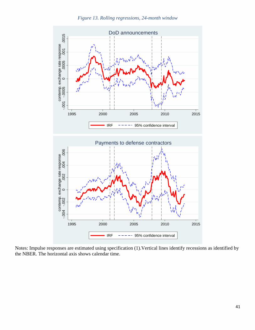
41  

Figure 13. Rolling regressions, 24-month window

Notes: Impulse responses are estimated using specification (1).Vertical lines identify recessions as identified by the NBER. The horizontal axis shows calendar time.

-.00

1-.

0005

0.0

005

.00

1.0

015

con

tem

p. e

xch

ange

rat

e re

spon

se

1995 2000 2005 2010 2015

IRF 95% confidence interval

DoD announcements

-.00

4-.

002

0.0

02

.00

4.0

06

con

tem

p. e

xch

ange

rat

e re

spon

se

1995 2000 2005 2010 2015

IRF 95% confidence interval

Payments to defense contractors

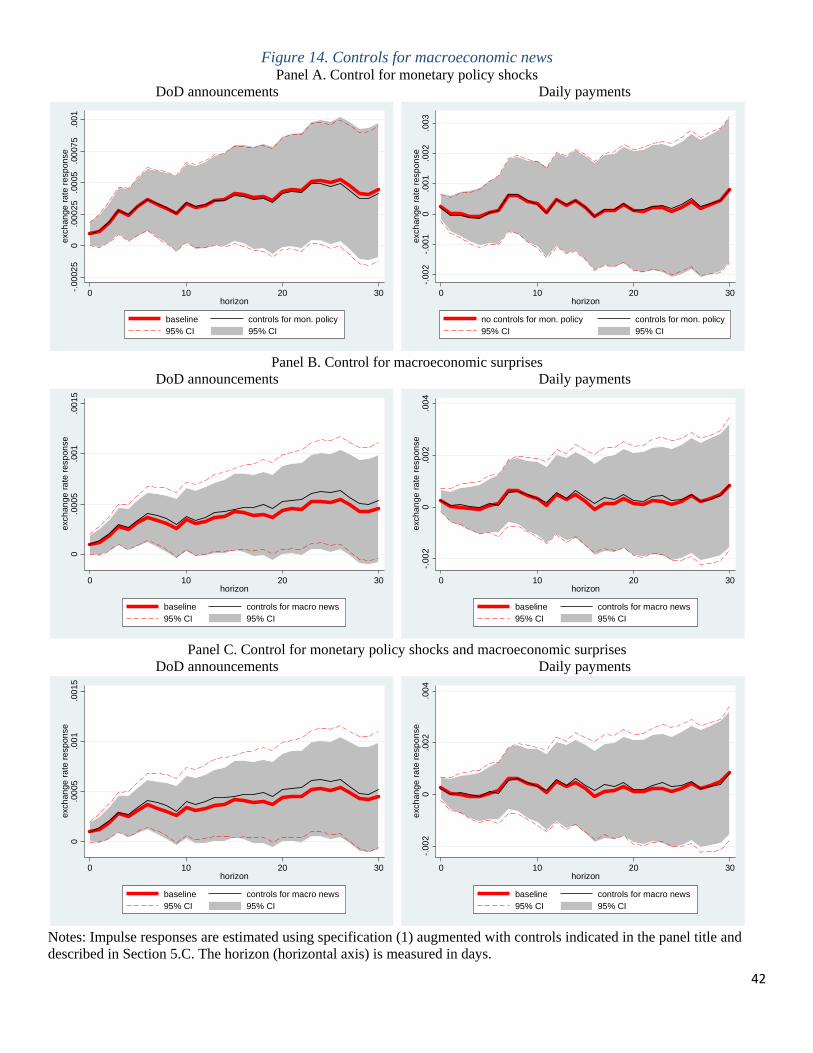
42  

Figure 14. Controls for macroeconomic news Panel A. Control for monetary policy shocks

DoD announcements Daily payments

Panel B. Control for macroeconomic surprises

DoD announcements Daily payments

Panel C. Control for monetary policy shocks and macroeconomic surprises

DoD announcements Daily payments

Notes: Impulse responses are estimated using specification (1) augmented with controls indicated in the panel title and described in Section 5.C. The horizon (horizontal axis) is measured in days.

-.00

025

0.0

002

5.0

005

.00

075

.00

1ex

chan

ge r

ate

res

pon

se

0 10 20 30horizon

baseline controls for mon. policy95% CI 95% CI

-.00

2-.

001

0.0

01

.00

2.0

03

exch

ange

ra

te r

esp

onse

0 10 20 30horizon

no controls for mon. policy controls for mon. policy95% CI 95% CI

0.0

005

.00

1.0

015

exch

ange

ra

te r

esp

onse

0 10 20 30horizon

baseline controls for macro news95% CI 95% CI

-.00

20

.00

2.0

04

exch

ange

ra

te r

esp

onse

0 10 20 30horizon

baseline controls for macro news95% CI 95% CI

0.0

005

.00

1.0

015

exch

ange

ra

te r

esp

onse

0 10 20 30horizon

baseline controls for macro news95% CI 95% CI

-.00

20

.00

2.0

04

exch

ange

ra

te r

esp

onse

0 10 20 30horizon

baseline controls for macro news95% CI 95% CI

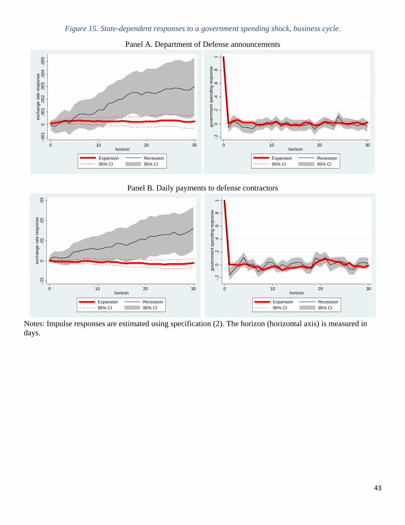
43  

Figure 15. State-dependent responses to a government spending shock, business cycle.

Panel A. Department of Defense announcements

Panel B. Daily payments to defense contractors

Notes: Impulse responses are estimated using specification (2). The horizon (horizontal axis) is measured in days.

-.00

10

.00

1.0

02

.00

3.0

04

.00

5ex

chan

ge r

ate

res

pon

se

0 10 20 30horizon

Expansion Recession95% CI 95% CI

-.2

0.2

.4.6

.81

gove

rnm

ent s

pen

din

g re

spon

se

0 10 20 30horizon

Expansion Recession95% CI 95% CI

-.01

0.0

1.0

2.0

3ex

chan

ge r

ate

res

pon

se

0 10 20 30horizon

Expansion Recession95% CI 95% CI

-.2

0.2

.4.6

.81

gove

rnm

ent s

pen

din

g re

spon

se

0 10 20 30horizon

Expansion Recession95% CI 95% CI

44  

Figure 16. State-dependent responses of the exchange rate to a government spending shock, business cycle and ZLB. Department of Defense announcements.

Panel A. Baseline

Panel B. Control for TED rate

Notes: Impulse responses are estimated using specification (3). The horizon (horizontal axis) is measured in days.

-.00

20

.00

2.0

04

.00

6.0

08

.01

exch

ange

ra

te r

esp

onse

0 10 20 30horizon

Expansion Recession95% CI 95% CI

Binding ZLB

-.00

2-.

001

0.0

01

.00

2.0

03

exch

ange

ra

te r

esp

onse

0 10 20 30horizon

Expansion Recession95% CI 95% CI

Non-binding ZLB

-.00

8-.0

06

-.00

4-.

002

0.0

02

.00

4.0

06

exch

ange

ra

te r

esp

onse

0 10 20 30horizon

Expansion Recession95% CI 95% CI

Binding ZLB-.

002

-.00

10

.00

1.0

02

.00

3.0

04

exch

ange

ra

te r

esp

onse

0 10 20 30horizon

Expansion Recession95% CI 95% CI

Non-binding ZLB

45  

Figure 17. State-dependent responses of the exchange rate to a government spending shock, business cycle and ZLB. Daily payments to defense contractors

Panel A. Baseline

Panel B. Control for TED rate

Notes: Impulse responses are estimated using specification (3). The horizon (horizontal axis) is measured in days.

-.02

-.01

0.0

1.0

2.0

3.0

4.0

5ex

chan

ge r

ate

res

pon

se

0 10 20 30horizon

Expansion Recession95% CI 95% CI

Binding ZLB

-.00

50

.00

5.0

1.0

15

.02

.02

5.0

3ex

chan

ge r

ate

res

pon

se

0 10 20 30horizon

Expansion Recession95% CI 95% CI

Non-binding ZLB

-.04

-.03

-.02

-.01

0.0

1.0

2.0

3.0

4.0

5ex

chan

ge r

ate

res

pon

se

0 10 20 30horizon

Expansion Recession95% CI 95% CI

Binding ZLB

-.00

50

.00

5.0

1.0

15

.02

.02

5.0

3ex

chan

ge r

ate

res

pon

se

0 10 20 30horizon

Expansion Recession95% CI 95% CI

Non-binding ZLB

46  

APPENDIX

47  

Appendix Figure 1. Impulse response of the exchange rate to a government spending shock, daily data, VAR.

Panel A. Department of Defense announcements. 

Panel B. Daily payments to defense contractors, U.S. Treasury.

Notes: The step (horizontal axis) is measured in days.

0

.0005

.001

0 10 20 30

irf0, TDC, dln_DTWEXM

95% CI cumulative orthogonalized irf

step

Graphs by irfname, impulse variable, and response variable

-.0005

0

.0005

.001

0 10 20 30

irf0, TDC, dln_DTWEXM

95% CI cumulative orthogonalized irf

step

Graphs by irfname, impulse variable, and response variable

48  

Appendix Figure 2. Response of the exchange rate to a government spending shock

Notes: Blanchard-Perotti identification amounts to putting government spending first in the Chosleki ordering. Ramey identification is based on the narrative approach applied to military spending. Ramey shocks are measured in percent of GDP. Impulse responses in both panels are calculated using direct projections. The list of controls include four lags of growth rate of real GDP, inflation rate (GDP deflator), government spending (corresponding series), and the exchange rate (see note to Figure 4). The horizon (horizontal axis) is measured in quarters.

-6-4

-20

2

0 1 2 3 4 5 6 7 8 9 10 11 12horizon (quarters)

IRF 95% confidence interval

Identification: Blanchard-Perotti

-2-1

01

23

0 1 2 3 4 5 6 7 8 9 10 11 12horizon

IRF 95% confidence interval

Identification: Ramey

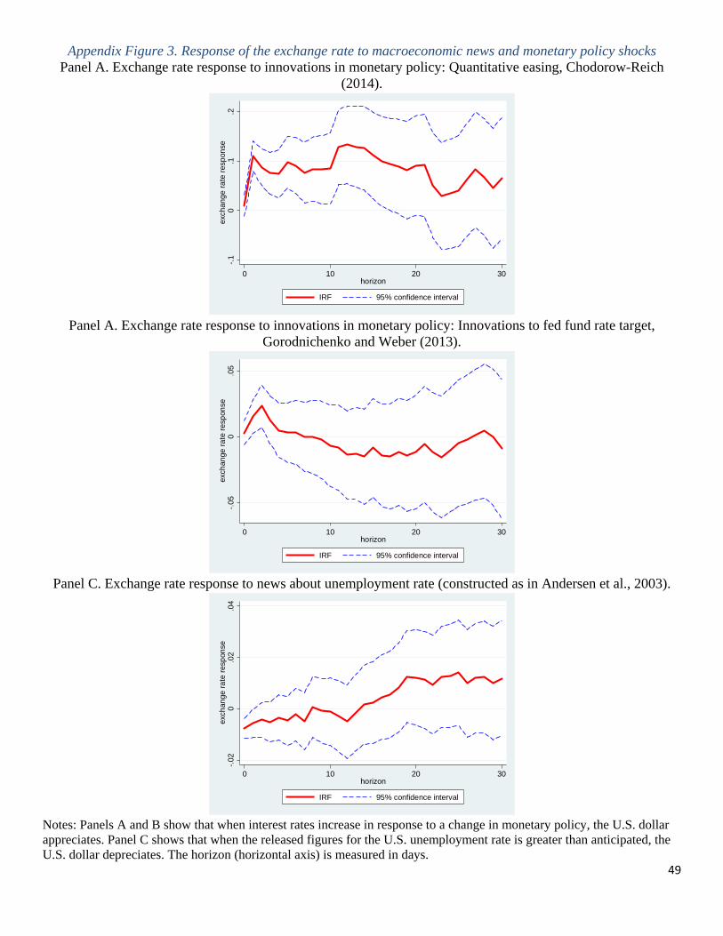
49  

Appendix Figure 3. Response of the exchange rate to macroeconomic news and monetary policy shocks Panel A. Exchange rate response to innovations in monetary policy: Quantitative easing, Chodorow-Reich

(2014).

Panel A. Exchange rate response to innovations in monetary policy: Innovations to fed fund rate target,

Gorodnichenko and Weber (2013).

Panel C. Exchange rate response to news about unemployment rate (constructed as in Andersen et al., 2003).

Notes: Panels A and B show that when interest rates increase in response to a change in monetary policy, the U.S. dollar appreciates. Panel C shows that when the released figures for the U.S. unemployment rate is greater than anticipated, the U.S. dollar depreciates. The horizon (horizontal axis) is measured in days.

-.1

0.1

.2ex

chan

ge r

ate

res

pon

se

0 10 20 30horizon

IRF 95% confidence interval

-.05

0.0

5ex

chan

ge r

ate

res

pon

se

0 10 20 30horizon

IRF 95% confidence interval

-.02

0.0

2.0

4ex

chan

ge r

ate

res

pon

se

0 10 20 30horizon

IRF 95% confidence interval

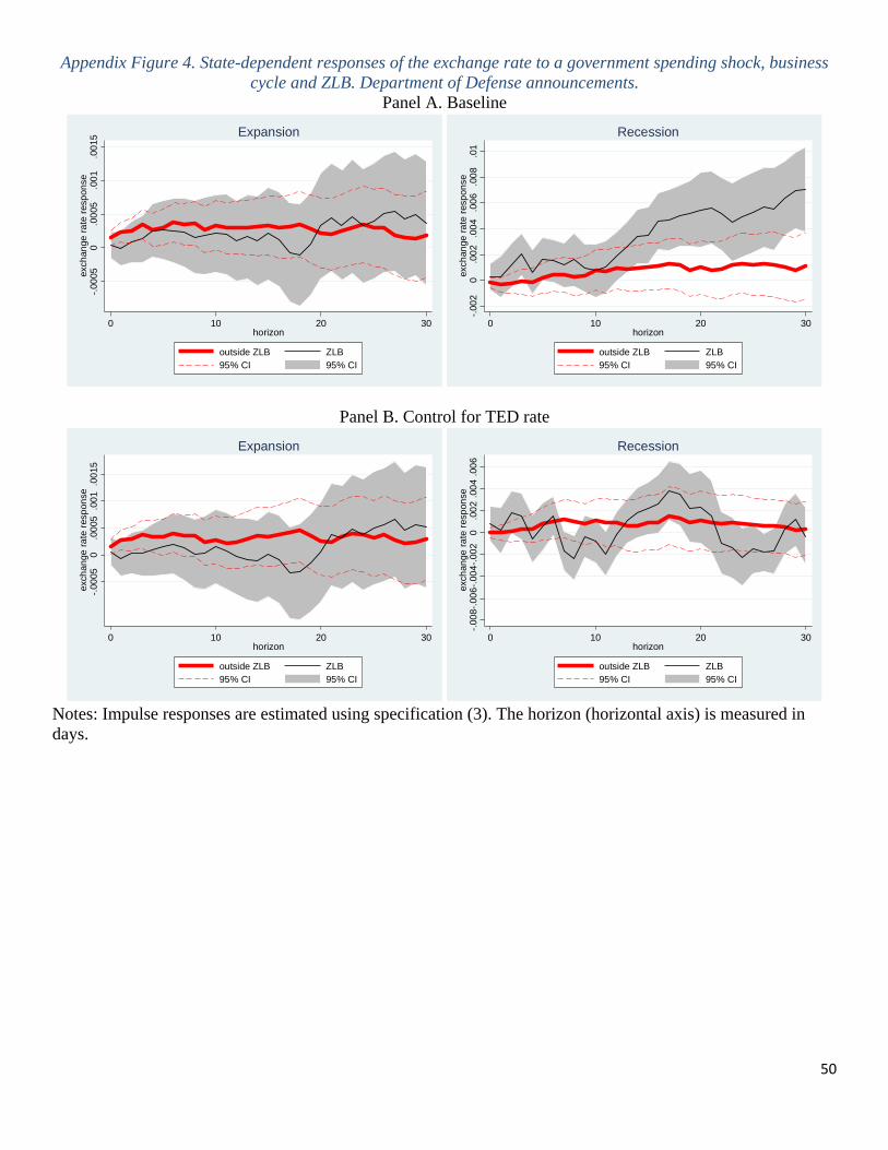
50  

Appendix Figure 4. State-dependent responses of the exchange rate to a government spending shock, business cycle and ZLB. Department of Defense announcements.

Panel A. Baseline

Panel B. Control for TED rate

Notes: Impulse responses are estimated using specification (3). The horizon (horizontal axis) is measured in days.

-.00

050

.00

05.0

01

.00

15ex

chan

ge r

ate

res

pon

se

0 10 20 30horizon

outside ZLB ZLB95% CI 95% CI

Expansion

-.00

20

.00

2.0

04

.00

6.0

08

.01

exch

ange

ra

te r

esp

onse

0 10 20 30horizon

outside ZLB ZLB95% CI 95% CI

Recession

-.00

050

.00

05.0

01

.00

15ex

chan

ge r

ate

res

pon

se

0 10 20 30horizon

outside ZLB ZLB95% CI 95% CI

Expansion

-.00

8-.0

06

-.00

4-.

002

0.0

02

.00

4.0

06

exch

ange

ra

te r

esp

onse

0 10 20 30horizon

outside ZLB ZLB95% CI 95% CI

Recession

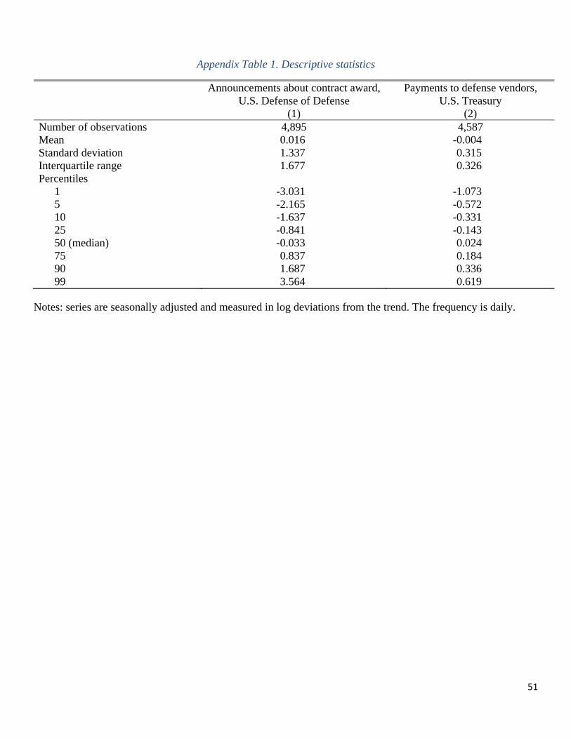
51  

Appendix Table 1. Descriptive statistics

Announcements about contract award, U.S. Defense of Defense

Payments to defense vendors, U.S. Treasury

(1) (2) Number of observations 4,895 4,587 Mean 0.016 -0.004 Standard deviation 1.337 0.315 Interquartile range 1.677 0.326 Percentiles

1 -3.031 -1.073 5 -2.165 -0.572 10 -1.637 -0.331 25 -0.841 -0.143 50 (median) -0.033 0.024 75 0.837 0.184 90 1.687 0.336 99 3.564 0.619

Notes: series are seasonally adjusted and measured in log deviations from the trend. The frequency is daily.