Langmuir 20005, in press

EFFECTS OF PULSED LOW FREQUENCY ELECTROMAGNETIC FIELDS ON WATER CHARACTERIZED BY LIGHT SCATTERING TECHNIQUES:

ROLE OF BUBBLES

Philippe Vallée1*, Jacques Lafait1, Laurent Legrand2, Pascale Mentré3, Marie-Odile

Monod4, Yolène Thomas5

1 Laboratoire d’ Optique des Solides (UMR CNRS 7601)

Université Pierre et Marie Curie,

Campus Boucicaut

140, rue de Lourmel, 75015 Paris, France

2 Groupe de Physique des Solides (UMR CNRS 7588)

Universités Pierre et Marie Curie (Paris 6) et Denis Diderot (Paris 7)

Campus Boucicaut

140, rue de Lourmel, 75015 Paris, France

3 UMR 8646 - MNHN

53 rue Buffon, 75005 PARIS, France

4 CEMAGREF

24, avenue des Landais - BP 50085

63172 AUBIERE Cedex, France

5 Institut Andre Lwoff IFR89

7, rue Guy Moquet-BP8

94801 Villejuif Cedex, France

*Corresponding author: phvallee@los.jussieu.fr

1

Abstract

Well-characterized purified water was exposed for 6 h to pulsed low-frequency weak

electromagnetic fields. After various time periods, nondegassed and degassed water samples

were analyzed by static light scattering. Just after electromagnetic exposure (day 0), a reduction

of over 20% in the maximum light scattering intensity at 488 nm wavelength in both

nondegassed and degassed samples was observed. By contrast, on day 12 the difference was

observed only in nondegassed water samples. The latter effect was attributed to the different

geometries of the containers combined with the basic origin of the whole phenomenon due to gas

bubbles present in water. By the use of dynamic light scattering, the bubble mean diameter was

estimated to be around 300 nm.

Our results suggest that the electromagnetic exposure acts on gas nanobubbles present in water

and emphasizes the role of the gas/liquid interface. The possibility that exposure to

electromagnetic fields disturbs the ionic double-layer that contributes to bubble stabilization in

water is discussed.

Keywords: Water, atmospheric environment, electromagnetic fields, light scattering, bubbles,

gas/water interface.

2

Introduction

During the past decade, there has been considerable investigation of the effects of static

magnetic and electromagnetic fields (EMF) on water or on the behavior of aqueous solutions and

suspensions1-4. The physicochemical properties of water (oxidation-reduction potential, pH, etc.)

may be altered by the magnetic and electromagnetic fields4,5. These changes depend on the field

intensity and/or frequency6,7. Despite intensive research, the mechanisms by which such

electromagnetic fields act on water are still a controversial issue. Indeed, it has been difficult to

obtain good experimental reproducibility, mainly due to variation in water composition and/or

environmental conditions. Among the different hypotheses put forward regarding the targets of

EMF, the colloid/water interface appears to be the most probable. For instance, Chibowski et al.8

studied the effects of EMF in the radio frequency range (44 MHz) on pH, conductivity and ζ

potentials of colloidal particles of different oxides. They observed noticeable oscillations in the ζ

potential for hours after treatment. Colic and Morse9, working with radio frequency EMF on

colloids in water, proposed that the electromagnetic exposure effect results from a perturbation

of gas/liquid interface and noted that degassing removes all of the observed effects (ζ potential,

turbidity, etc). These changes persist for hours and even days10. Fesenko et al.5, treating triply

distilled deionized water with microwaves, suggested that the EMF might act on gas dissolved in

water. Eberlein11,12 proposed a quantum vacuum radiation explanation of the effect based on the

influence of an oscillating EMF on the gas/water interface.

Previous studies from our laboratory13 and others14 show that species arising from

container/content interactions affect the physicochemical properties of water. We developed and

present in this paper new experimental procedures to investigate the effect of pulsed low-

frequency EMF on water. In particular, special attention has been paid to (1) water purification

and physicochemical characterization and (2) environmental conditions (atmospheric,

3

electromagnetic, and acoustic). Moreover, glassware was made of pure fused optical silica in

order to minimize the release of compounds from the containers. Experiments were also carried

out to explore the influence of gas bubbles on the EMF effect by using static and dynamic light

scattering. Finally, we discuss different mechanisms for the action of the electromagnetic fields,

in particular via a mechanical action on the ionic charges present around gas bubbles.

1. Experimental Section

1.1 Materials

Water

Water used in the experiments described below was freshly prepared from Paris tap water

(pressure 6 bar) after two purification steps using: (1) an inverse osmosis apparatus (Millipore,

Rios III) that eliminates molecules between 0.2 and 1 nm as well as 97% of ionic substances and

(2) a final purification apparatus (Millipore, SimplicityTM) equipped with an ultrafilter

(Millipore, Pyrogard D, size cutoff of 13,000 Da) which eliminates the remaining organic

compounds ≥ 5-10 nm. At the end of the procedure, the purified water was apyrogenic according

to the manufacturer and the resistivity was measured to be 18.2 MΩ.cm at 25 °C.

Glassware

All glassware was made of pure fused optical silica (Heraeus, Suprasil) in order to minimize

container/content interaction13,14. Optical cells (Hellma, Qs111, of volume: 3.5 mL and cross

section: 1 cm2), were closed with a pure fused silica cap. Glassware was thoroughly washed with

spectroscopy grade ethanol (Merck Uvasol, purity 0.999) to remove any surface active material

and then put in a clean oven at 80°C for 15 min. Just before use, the optical cells were rinsed

with purified water. A special glassware apparatus made of two compartments, a round beaker

connected to an optical cell, was used to degas water.

4

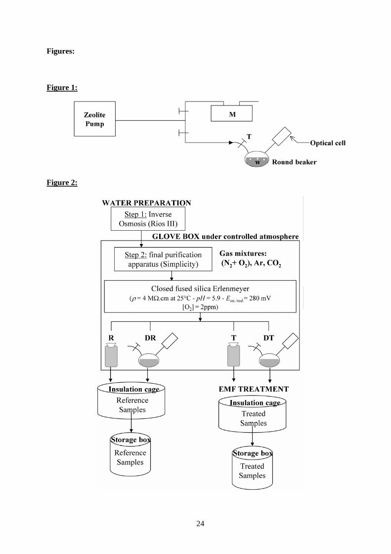
Glovebox

To ensure a controlled atmosphere, samples were prepared inside a glovebox (Jacomex,

Altuglass model B003). To reconstitute atmospheric air, argon (N56, Air Liquide), carbon

dioxide (N48, Air Liquide), oxygen, and nitrogen (Air N57 Pol, Air Liquide) were filtered

through a 0.2 µm filter (Osmonics, Teflon Calyx Capsule) and then introduced into the

glovebox. To avoid contamination from outside, a pressure 3 mbar above ambient was

maintained. Relative humidity (60 ± 2%) and carbon dioxide (310 ± 20 ppm) were measured

using a Vaisala GM70 hand-held meter (Vaisala, calibrated probe, humidity: HMP75 and carbon

dioxide: GMP70).

Insulation cages and storage boxes

To control environmental conditions during the exposure to electromagnetic fields, samples were

kept in thermally, acoustically, and magnetically shielded containers (diameter 700 mm, 500 mm

high). Thermal and acoustic insulation were achieved by using multilayers of various polymers

(Illbruck Company, EPDM, density: 8kg/m3, 20 mm thick; melamine resin, density: 11kg/m3, 20

mm thick and bitumen mass, density 10kg/m3, 3 mm thick). For magnetic insulation we used a

double layer of mu-metal (Meca-Magnetic, two foils of “Mumetal”, each 1mm thick). According

to the manufacturer, the ambient magnetic field intensity (0.1 mT root mean square (rms), ac, 50

Hz) is reduced by a factor of 850 (≈ 58 dB). A Faraday cage of copper foil (2 mm thick) was

used for electrical insulation.

In addition, two cylindrical storage boxes made of mu-metal (diameter 80 mm, 105 mm high, 2

mm thick) were built to shield the closed samples. Each storage cylinder was finally put into a

Thermos® box.

5

1.2 Water treatments

Electromagnetic exposure

Optical cells containing purified water were placed in one of the two insulation cages and

exposed for 6 h to pulsed (duration 30 s) electromagnetic fields generated by a solenoid coil

(diameter 50 mm, 80 mm high, copper wire, 4367 turns/m, self-inductance L = 3 mH, ohmic

resistance 3 Ω). The electric signal applied to the coil, provided by a programmable function

generator (Agilent 33120A), was composed of three successive sinusoidal pulse trains in the

frequency range from 10 to 500 Hz. Optical cells were placed in a vertical position in the center

of the coil supplied by a 250 mA (rms) current. The calculated rms magnetic field density at the

center of the coil is ≈ 1 mT and, according to Faraday’s law, the maximum induced electric field

is 4.1 mV/m. Reference (untreated) optical cells were placed in the other insulation cage under

the same conditions except they were not exposed to the electromagnetic fields. After the

electromagnetic exposure, optical cells (reference (R) and treated (T)) were transferred and kept

in separate storage boxes. The temperature has been measured during the electromagnetic

exposure, by using a chromel/alumel thermocouple (∆T was less than 0.01 °C).

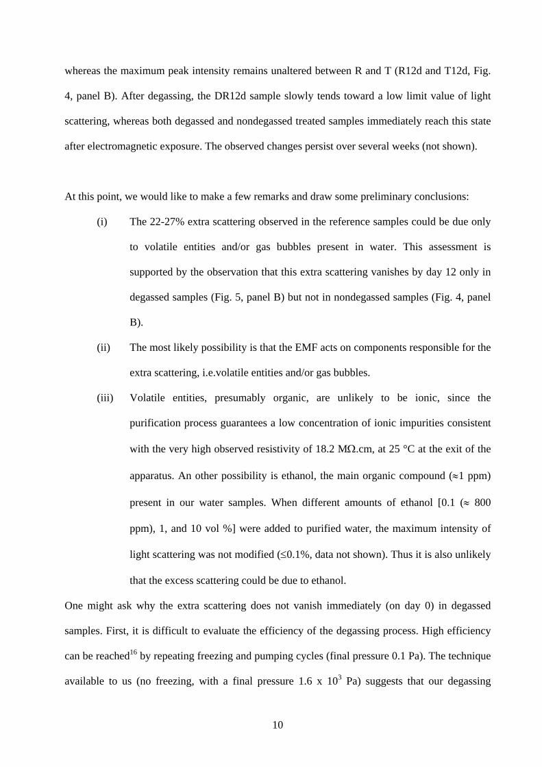
Degassing process (Fig. 1)

A zeolite pump was used to degas purified water (20 min, at a pressure of 1.6x103 Pa, as

measured by a Comark, manometer model C9555). Degassing was done prior to exposure to

electromagnetic fields in the dedicated glassware (1/7 of the total volume filled with water) as

described above. After pumping, degassed water was transferred from one compartment of the

glassware (Suprasil round beaker) to the connected optical cell compartment. Degassed reference

water (DR) and degassed treated water (DT) samples are thus ready for optical measurements.

Note that, in nondegassed samples, the optical cells were filled to the top with water and sealed

with the cap.

6

1.3 Measurements

Physicochemical water analysis

All the measurements using a multiparametric system (Fisher Scientific, Consort C835

multimeter) were always done in the glovebox, in the same order: conductivity/temperature,

oxygen content, pH, and oxidation-reduction potential (ORP). Multi-meter data were logged on a

computer. For conductivity measurements the apparatus was equipped with a specific electrode

of cell constant K = 0.1 cm-1 for low ionic concentration solutions with automatic temperature

correction (Pt1000) and calibrated with two ionic strength solutions (Hanna Instruments, 84 and

1413 µS cm-1 at 25 °C). pH measurements were done using a combined electrode (Metrohm, LL-

Aquatrode) adapted for pure water. The electrode was calibrated using a test kit buffer (Scott-

Geräte). For ORP measurements we used a combined electrode with platinum ring (Fisher

Scientific, N90417), and for oxygen measurements, we used a combined electrode for

oxygen/temperature (Fisher Scientific, N98338). The ORP probe was calibrated using a redox

solution of 470 mV (Scott-Geräte, Pt-Ag/AgCl at 25 °C), and the oxygen probe was calibrated

for 100% oxygen present in air. The total organic compounds (TOC) concentration was

measured by an A10 monitor (Anatel, Millipore). The accuracy was 15% in the range 2-1000

ppb. To minimize the fluctuations of TOC residual content (≈ 0.05 ppm), a small organic

compound, here ethanol, was added (≈ 0.95 ppm) during water preparation.

Ambient fields

Static magnetic field measurements were performed inside the insulation cages with a

low field axial probe (Bartington Instruments Ltd., model Mag B), positioned at 60° relative to

the horizontal, connected to a Mag-01H apparatus (Bartington Instruments Ltd). Fluctuating

magnetic fields were measured along three axes over a frequency range of 5 Hz to 400 kHz with

the probe of an Esm-100 meter (Maschek) placed close to the exposure area. In the absence of

7

signal, the values in the coil were: static magnetic field 9.9 µT, fluctuating magnetic field (in the

range 5 Hz to 400 kHz) 16 nT, and fluctuating residual electric field (mostly 50 Hz, isotropic)

6.3 V/m. It should be noted that the applied pulsed magnetic field (≈1 mT) was far above the

magnetic fields, both fluctuating (16 nT) and static (less 10 µT). The maximum induced electric

field produced by the applied electromagnetic field, 4.1 mV/m, was very small as compared to

the environmental electric field (a few volts per meter).

Procedure and physicochemical characterization of samples

For good homogeneity among different samples, water coming from the SimplicityTM

apparatus was stored for 25 min in a closed Erlenmeyer 250 mL flask (see Figure 2). Then, water

was quickly poured into the optical cells which were filled to the top. Optical cells were closed

with a silica ground cap and sealed with Parafilm. During this storage period, an aliquot sample

was analyzed: resistivity: 4.0 MΩ.cm at 25 °C, TOC content: ≈ 1 ppm (mainly ethanol), pH: 5.9,

redox potential: 280 mV, and oxygen content: 2 ppm.

Static light scattering analysis

Static light scattering was measured at 90° to the incident beam under monochromatic

illumination. The light source was an argon laser (Coherent, Innova 300), with a wavelength λ =

488 nm, a continuous wave power of 100 mW, vertically polarized, with spot diameter 5 mm,

and incident on the middle of the cell. The signal was collected at 90° to the incident beam by an

optical fiber located 15 mm from the cell and analyzed using a Jobin-Yvon HR460 double

monochromator spectrometer equipped with a multichannel CCD detector (Spectraview-2D,

2000 pixels). The resolution was 4 nm/pixels with a 300 µm slit. The wavelength explored range

was between 435 and 835 nm. The incident power at the sample was measured before and after

each scan and for each sample. The acquisition time was 2 s with 60 accumulated scans. All data

were recorded at room temperature (21.0 ± 0.5 °C).

8

Dynamic light scattering analysis

Dynamic light scattering can be used to determine the size of particles via their motion in

a liquid. In the case of dilute solutions of monodisperse particles, with a small size as compared

to the wavelength (Rayleigh scattering), for the intensity I(t) the autocorrelation function G(τ) =

)()( τ+tItI takes a simple form15. The τ dependent part of G(τ) is exp (- 2Dq2τ) where D is

the apparent diffusion coefficient of the particles in the liquid and q is the wave vector.

Here ⎟⎠⎞

⎜⎝⎛=

2sin

4 θλ

πnq solvent , (1)

where nsolvent is the refractive index of the solvent, λ is the wavelength of the incident beam, and

θ is the angle at which the intensity is measured.

From the intensity autocorrelation function measured at different angles θ, i.e., for different q

values, one can determine the apparent diffusion coefficient D. In the absence of interactions

between scatterers, the Stokes-Einstein equation relates the diffusion coefficient to the

hydrodynamic radius (RH)15:

DπηTkR

solvent

BH 6

= , (2)

where ηsolvent is the viscosity of the solvent, T is the temperature and kB is the Boltzmann

constant.

In the case of spherical particles the hydrodynamic radius can be assumed to be the geometric

radius of the moving particles. This technique is usually successfully applied to the

determination of the size of colloidal particles. We extend its use to study bubbles in water. We

used the apparatus commercialized by Brookhaven Instrument Corporation (Model Bi-9000AT

digital correlator, BI200SM goniometer), illuminated by a krypton laser (Spectra Physics,

Stabilite 2017, λ=647 nm, power 300 mW, vertically polarized). The laser beam was focused

(beam waist 200 µm) on the center of the optical cells. The optical cell was placed in the center

9

of a cylindrical vat filled with an index matching liquid, namely anhydrous

decahydronaphthalene (Sigma, n = 1.474). The scattered light was collected in three directions at

60°, 90° and 120° from the incident beam, by a PM detector with a diaphragm of 400 µm

diameter. The sampling time τ of the correlator was set from 25 µs to 7 x 106 µs. For each angle,

the acquisition time was 15 min. All measurements were recorded at room temperature (24.5 ±

0.5°C).

2. Results and discussion

Nondegassed and degassed water samples were exposed for 6 h to pulsed low-frequency

electromagnetic fields. Static light scattering measurements were performed on day 0 and on day

12 after treatment. At all other times, each sample was stored in a separate insulation box. The

very good stability of measurement conditions within the same experiment and the comparison

of couples (reference and treated samples), permits the direct comparison of their spectra without

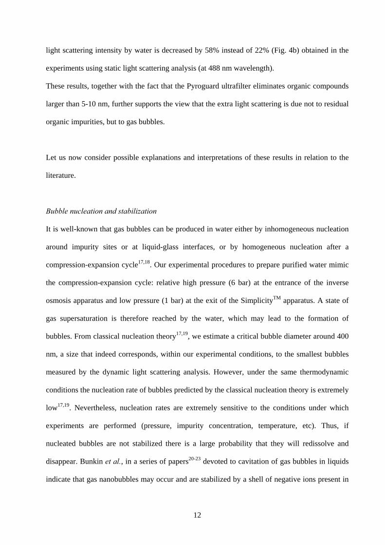
any normalization. We have observed in Raman scattering experiments (not presented in this

study) that Raman spectra were affected neither by electromagnetic exposure, nor by degassing,

in either intensity or band position. This is illustrated in Fig. 3, where the maximum intensity of

the Raman peak observed at 585 nm in the measurements of couples remains constant. Typical

results (among five different samples prepared on different dates) for static light scattering

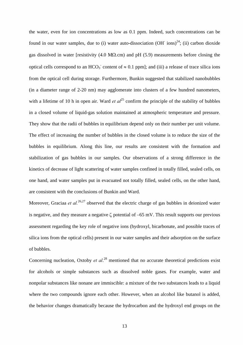
experiments before and after exposure to electromagnetic fields are presented in Figs. 4 and 5.

After electromagnetic exposure, a decrease of 27% (standard deviation 5%) on day 0 (Fig. 4,

panel A) and of 22% (standard deviation 5%) on day 12 (Fig. 5, panel A) in the maximum light

scattering intensity was observed in both nondegassed (R and T) and degassed samples (DR and

DT), respectively. The difference between the maximum scattering peak intensity of DR and DT,

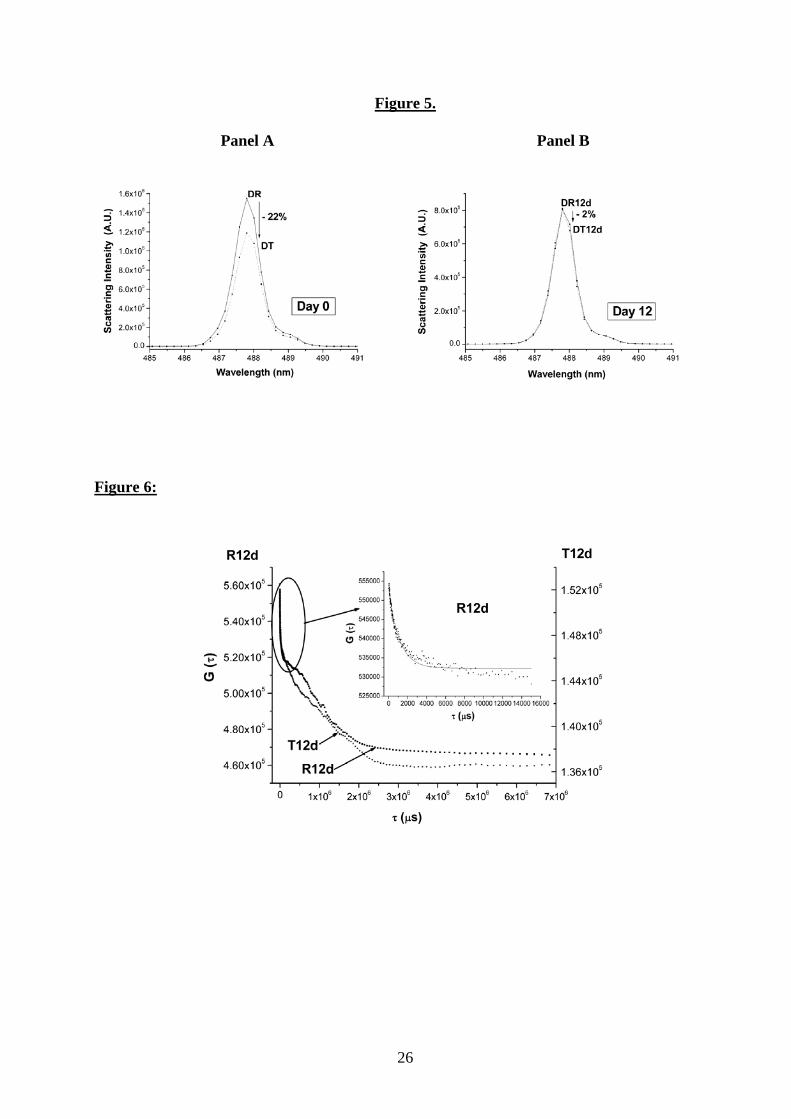
measured just after treatment, vanishes 12 days later (DR12d and DT12d, Fig. 5, panel B),

10

whereas the maximum peak intensity remains unaltered between R and T (R12d and T12d, Fig.

4, panel B). After degassing, the DR12d sample slowly tends toward a low limit value of light

scattering, whereas both degassed and nondegassed treated samples immediately reach this state

after electromagnetic exposure. The observed changes persist over several weeks (not shown).

At this point, we would like to make a few remarks and draw some preliminary conclusions:

(i) The 22-27% extra scattering observed in the reference samples could be due only

to volatile entities and/or gas bubbles present in water. This assessment is

supported by the observation that this extra scattering vanishes by day 12 only in

degassed samples (Fig. 5, panel B) but not in nondegassed samples (Fig. 4, panel

B).

(ii) The most likely possibility is that the EMF acts on components responsible for the

extra scattering, i.e.volatile entities and/or gas bubbles.

(iii) Volatile entities, presumably organic, are unlikely to be ionic, since the

purification process guarantees a low concentration of ionic impurities consistent

with the very high observed resistivity of 18.2 MΩ.cm, at 25 °C at the exit of the

apparatus. An other possibility is ethanol, the main organic compound (≈1 ppm)

present in our water samples. When different amounts of ethanol [0.1 (≈ 800

ppm), 1, and 10 vol %] were added to purified water, the maximum intensity of

light scattering was not modified (≤0.1%, data not shown). Thus it is also unlikely

that the excess scattering could be due to ethanol.

One might ask why the extra scattering does not vanish immediately (on day 0) in degassed

samples. First, it is difficult to evaluate the efficiency of the degassing process. High efficiency

can be reached16 by repeating freezing and pumping cycles (final pressure 0.1 Pa). The technique

available to us (no freezing, with a final pressure 1.6 x 103 Pa) suggests that our degassing

11

efficiency is relatively low. This could explain both the persistence of extra scattering in

degassed samples (Fig. 5, panel A) and the agreement in light scattering intensities of

nondegassed and degassed reference samples for day 0 (Fig. 4 and 5, panel A). Second, the

geometry of glassware used for degassed samples (see above and Figure 1) allows water to

slowly degas by pulling the remaining gases into the space above the liquid and thus reach a new

equilibrium state in the presence of a low-pressure atmosphere. This process can be inhibited or

delayed in nondegassed cells that were totally filled.

To further explore the possible role of gas bubbles, water samples treated (T12d) or not (R12d)

were analyzed using dynamic light scattering, which gives quantitative information on the size of

the scatterers through the measurement of the time evolution of the intensity autocorrelation

function G(τ) (see part Dynamic light scattering analysis). The intensity autocorrelation function

of sample R12d measured at 120° (Fig. 6) presents a two-step temporal decay, characteristic of

the existence of two size distributions with very different mean sizes. In this particular case,

analysis of the signal G(τ) at the lowest delay times τ explored, leads to a determination of the

mean decay time for the smaller sized particles. This time is close to 1.3 ms (see Figure 6, inset).

In our experiment this value corresponds to a mean diameter for the scatterers of around 300 nm.

Note that simultaneous analysis of both distributions is difficult to perform mainly because of the

width (presumably due to polydispersity) and also because possible interactions between

scatterers are not easily taken into account in the model. The other main point is that, after

electromagnetic exposure, a partial vanishing of the small size particle distribution was observed

(curve T12d, cf. Fig. 6). Interestingly, the device we used for dynamic light scattering also

permits measurement of the average static light scattering at wavelength 647 nm. Moreover, it

permits elimination of the contribution of large scatterers occasionally crossing the illumination

beam. Under this condition, the effect of exposure to electromagnetic fields in the maximum

12

light scattering intensity by water is decreased by 58% instead of 22% (Fig. 4b) obtained in the

experiments using static light scattering analysis (at 488 nm wavelength).

These results, together with the fact that the Pyroguard ultrafilter eliminates organic compounds

larger than 5-10 nm, further supports the view that the extra light scattering is due not to residual

organic impurities, but to gas bubbles.

Let us now consider possible explanations and interpretations of these results in relation to the

literature.

Bubble nucleation and stabilization

It is well-known that gas bubbles can be produced in water either by inhomogeneous nucleation

around impurity sites or at liquid-glass interfaces, or by homogeneous nucleation after a

compression-expansion cycle17,18. Our experimental procedures to prepare purified water mimic

the compression-expansion cycle: relative high pressure (6 bar) at the entrance of the inverse

osmosis apparatus and low pressure (1 bar) at the exit of the SimplicityTM apparatus. A state of

gas supersaturation is therefore reached by the water, which may lead to the formation of

bubbles. From classical nucleation theory17,19, we estimate a critical bubble diameter around 400

nm, a size that indeed corresponds, within our experimental conditions, to the smallest bubbles

measured by the dynamic light scattering analysis. However, under the same thermodynamic

conditions the nucleation rate of bubbles predicted by the classical nucleation theory is extremely

low17,19. Nevertheless, nucleation rates are extremely sensitive to the conditions under which

experiments are performed (pressure, impurity concentration, temperature, etc). Thus, if

nucleated bubbles are not stabilized there is a large probability that they will redissolve and

disappear. Bunkin et al., in a series of papers20-23 devoted to cavitation of gas bubbles in liquids

indicate that gas nanobubbles may occur and are stabilized by a shell of negative ions present in

13

the water, even for ion concentrations as low as 0.1 ppm. Indeed, such concentrations can be

found in our water samples, due to (i) water auto-dissociation (OH- ions)24; (ii) carbon dioxide

gas dissolved in water [resistivity (4.0 MΩ.cm) and pH (5.9) measurements before closing the

optical cells correspond to an HCO3- content of ≈ 0.1 ppm]; and (iii) a release of trace silica ions

from the optical cell during storage. Furthermore, Bunkin suggested that stabilized nanobubbles

(in a diameter range of 2-20 nm) may agglomerate into clusters of a few hundred nanometers,

with a lifetime of 10 h in open air. Ward et al25 confirm the principle of the stability of bubbles

in a closed volume of liquid-gas solution maintained at atmospheric temperature and pressure.

They show that the radii of bubbles in equilibrium depend only on their number per unit volume.

The effect of increasing the number of bubbles in the closed volume is to reduce the size of the

bubbles in equilibrium. Along this line, our results are consistent with the formation and

stabilization of gas bubbles in our samples. Our observations of a strong difference in the

kinetics of decrease of light scattering of water samples confined in totally filled, sealed cells, on

one hand, and water samples put in evacuated not totally filled, sealed cells, on the other hand,

are consistent with the conclusions of Bunkin and Ward.

Moreover, Graciaa et al.26,27 observed that the electric charge of gas bubbles in deionized water

is negative, and they measure a negative ζ potential of –65 mV. This result supports our previous

assessment regarding the key role of negative ions (hydroxyl, bicarbonate, and possible traces of

silica ions from the optical cells) present in our water samples and their adsorption on the surface

of bubbles.

Concerning nucleation, Oxtoby et al.28 mentioned that no accurate theoretical predictions exist

for alcohols or simple substances such as dissolved noble gases. For example, water and

nonpolar substances like nonane are immiscible: a mixture of the two substances leads to a liquid

where the two compounds ignore each other. However, when an alcohol like butanol is added,

the behavior changes dramatically because the hydrocarbon and the hydroxyl end groups on the

14

alcohol molecules allow them to interact effectively with both hydrophobic and hydrophilic

liquids. The typical characteristic of such amphiphilic molecules is that they insert themselves in

nonpolar/hydrophilic compound interfaces and can therefore decrease the surface tension28. In

our experiments, one can assume a similar ternary nucleation (gas + water + amphiphilic

molecule), where the role of the amphiphilic molecule would be played by ethanol and most of

the constituents of bubbles (N2, O2, Ar) are hydrophobic. Moreover, one can assume that ethanol

can also play a role in bubble stabilization by the slight decrease of the surface tension at the

bubble/liquid interface (γb/w ≈ 71 mN m-1 at 20 °C), in particular via the ionization of hydrated

OH groups.

Along this line, Usui and Healy,29 investigating the ζ potential at the air-aqueous solution

interface of insoluble monolayers of long chain alcohols, conclude that the long chains insert at

the air-water interface and that the hydrophilic OH groups are directed toward the water, while

hydrocarbon groups are directed toward air. They attribute the measured negative ζ potential to

the dissociation of protons from water molecules that hydrate the OH groups of the alcohols

present at the air-water interface29. Despite a shorter hydrocarbon chain, ethanol present in our

samples could behave in a similar manner and thus be negatively charged. This negative charge

of ethanol preferentially adsorbs on bubbles and may contribute to the stabilization of bubbles in

our water samples.

Let us now envision different mechanisms for the action of electromagnetic fields on the gas

bubble/water interface.

Possible action of EMF

Some conclusions by Colic and Morse10,30,31, working with oscillating electromagnetic fields at

radio frequencies on aqueous solutions, should be recalled: (i) EMF can influence a gas-liquid

15

interface; (ii) degassing removes all of the observed effects of EMF; (iii) EMF produces effects

stable for hours. Despite different experimental conditions such as frequency (MegeHertz versus

Hertz to kiloHertz), and colloidal particles instead of gas bubbles, most of their conclusions are

consistent with our observations. This analogy is supported by the fact that bubbles in water

behave like a colloidal solution. Indeed, colloidal solutes, like bubbles, are particles on which

ions are adsorbed. Around the adsorbed ions a shell of counterions (i.e., a diffuse layer) is also

present. As described and discussed above, the adsorption of ions by gas bubbles and the

formation of a shell of counterions participate in the stabilization of bubbles. Electromagnetic

fields may have an important action on these ions. This effect has been already observed

indirectly by several authors studying the ζ potential10,30,32,33: For instance, Higashitani et al.32

observed the effect of low static magnetic fields on nonmagnetic colloids of polystyrene particles

in electrolyte solutions that they interpret as a modification of the ionic adsorbed layer.

Let us now speculate about the mechanism of EMF action on the ionic concentration responsible

for the stability of the bubbles.

In our study, one can infer the key role of HCO3- ions (coming from CO2 gas dissolved in our

water), and indirectly of OH- ions. From the value (5.9) of the pH of our samples, and the

following equation:

CO2(solution) + 2H2O HCO3- + H3O+ , (3)

one can calculate the HCO3- concentration with pKa of [CO2(solution)]/[HCO3

-] of 6.4); we find

[HCO3-] = 0.077 ppm under our conditions, i.e. two orders of magnitude larger than [OH-].

At carbon dioxide partial pressure comparable to ours, Liu et al.34 showed that the conversion of

CO2 (equation 3) mainly occurs in the diffusion boundary (Gouy-Chapman) layer, adjacent to

the surface of the colloids. This conversion depends on the thickness of the Gouy-Chapman

layer.

16

Interestingly, Beruto et al.35 applying low-frequency electromagnetic fields with characteristics

closed to ours (250 µT, square wave at 75 Hz) on aqueous electrolyte solutions, demonstrate that

they have the same effect as degassing on the pH and surface tension of their solutions.

Let us now envisage in more details the effect of degassing on the ionic concentration.

In our case, the degassing of the CO2(solution) from the interface is an irreversible process:

CO2(solution) CO2(gas) (4)

which involves, according to equation (3), a decrease of HCO3- in the solution. This tends to

neutralize the interfacial area. Thus, in our experiments pulsed low frequency EMF may act on

the bubble/water interface, leading to the destabilization of bubbles, mostly by disturbing the

ionic balance between the shell of adsorbed negative ions and counterions.

Several authors36,37 invoke the Lorentz force as the force acting in this destabilization.

Gamayunov36 showed that the Lorentz force causes a local deformation of the electric double

layer of particles or air bubbles of various sizes, moving with a carrier liquid in a static magnetic

field (around 75 mT). This deformation temporarily lowers the ionic electrostatic repulsion

barrier and results in the coalescence of gas bubbles. Furthermore, Lipus et al37 also explain the

destabilizing effect of treatment with a static magnetic field (range 0.05 – 1T) on the dispersion

of particles or bubbles in water via the neutralization of the surfaces of the dispersed phase. They

attribute the origin of the surface neutralization to the Lorentz force inducing a shift of

counterions from the Gouy-Chapman into the Stern layer.

Finally, others authors invoke the magnetic properties of water molecules to explain the action of

EMF on the bubble/water interface38,39. Beyond the classical property of the water molecule as a

magnetic dipole, several authors6,40,41 envisioned the possible role of the two nuclear spin

isomers: ortho- and para- water in the trapping on interfaces.

17

These different models are not mutually exclusive. Yet, at present, we favor the idea that the

EMF mainly acts via the ionic double layer present at the gas bubble/water interface. Additional

studies will be needed to clarify these issues.

4. Conclusions

Several points emerge from this study:

(i) A thorough process of water sample preparation and characterization has been developed

to investigate the effect of pulsed low frequency electromagnetic fields on pure water.

Environmental conditions as well as water and gas purity were also severely controlled.

(ii) Static light scattering analysis, together with the degassing of water sample, allowed us

to point out the action of electromagnetic fields on gas bubbles present in our water

samples. Exposure to electromagnetic fields resulted in a reduction in the maximum

elastic scattering intensity and a vanishing (or decrease) of gas bubbles.

(iii) Dynamic light scattering analysis allowed us to estimate the diameter of bubbles to be

around 300 nm.

Together, these results suggest that the pulsed low frequency electromagnetic treatment acts on

the gas/liquid interface, mainly by disturbing the ionic double layer that stabilizes nanobubbles

in water.

They also open interesting perspectives in biology. Indeed, biological systems are organized into

nanocompartments within the size range of gas bubbles we observe. Within the framework of

our results, one can infer that interface effects related to the specific distributions of ions in water

at the boundary of these compartments may play a key role in biological processes42,43.

18

Acknowledgements

This work is part of a Ph.D. thesis prepared by Ph. Vallée and was supported by a grant from the

Odier Fondation.

The assistance of R. Nectoux, Ph. Camps, and G. Vuye in the design and realization of the

electromagnetic device is highly appreciated. We thank B. Démarets, S. Chenot, and M.

Lempereur for technical assistance. We are indebted to C. Naud and C. Barthou for help in light

scattering measurements and procedures. We are especially grateful to R. Strasser, B. Cabane, B.

Guillot, G. Liger-Belair, and M. Odier for helpful advice and fruitful discussions. We also thank

David Wood for editing the manuscript.

19

References

(1) Coey, J. M. D.; Cass, S. J. Magn. Magn. Mater. 2000, 209, 71-74.

(2) Busch, K. W.; Busch, M. A. Desalination 1997, 109, 131-148.

(3) Gabrielli, C.; Jaouhari, R.; Maurin, G.; Keddam, M. Water Res. 2001, 35, 3249-

3259.

(4) Yamashita, M.; Duffield, C.; Tiller, W. A. Langmuir 2003, 19, 6851-6856.

(5) Fesenko, E. E.; Gluvstein, A. Y. FEBS Lett. 1995, 367, 53-55.

(6) Ozeki, S.; Wakai, C.; Ono, S. J. Phys. Chem. 1991, 95, 10557-10559.

(7) Oshitani, J.; Uehara, R.; Higashitani, K. J. Colloid Interface Sci. 1999, 209, 374-

379.

(8) Chibowski, E.; Holysz, L. Colloids Surf. 1995, 101, 99-101.

(9) Colic, M.; Morse, D. Colloids Surf. 1999, 154, 167-174.

(10) Colic, M.; Morse, D. Langmuir 1998, 14, 783-787.

(11) Eberlein, C. Phys. Rev. Lett. 1986, 76, 3842–3845.

(12) Eberlein, C. Phys. Rev. A 1996, 53, 2772-2787.

(13) Vallée, P.; Lafait, J.; Ghomi, M.; Jouanne, M.; Morhange, J. F. J. Mol. Struct.

2003, 651-653, 371-379.

(14) Elia, V.; Niccoli, M. J. Therm. Anal. Calorim. 2004, 75, 815-836.

(15) Teraoka, I. Polymer solutions: an introduction to physical properties; John Wiley

& Sons Inc.: New York, 2002; Chapter 3.

(16) Pashley, R. M. J. Phys. Chem. B 2003, 107, 1714-1720.

(17) Liger-Belair, G. Ann. Phys. 2002, 27, 1-106.

(18) Liger-Belair, G.; Vignes-Adler, M.; Voisin, C.; Robillard, B.; Jeandet, P.

Langmuir 2002, 18, 1294-1301.

20

(19) Epstein, P. S.; Plesset, M. S. J. Chem. Phys. 1950, 18, 1505-1509.

(20) Bunkin, N. F.; Bunkin, F. V. Sov. Phys. JETP 1992, 74, 271-8.

(21) Bunkin, N. F.; Lobeyev, A. V. Phys. Lett., A 1997, 229, 327-33.

(22) Bunkin, N. F.; Lobeev, A. V. Jetp Lett. 1995, 62, 685-688.

(23) Bunkin, N. F.; Kochergin, A. V.; Lobeyev, A. V.; Ninham, B. W.; Vinogradova,

O. I. Colloids surf. 1996, 110, 207-212.

(24) Geissler, P. L.; Dellago, C.; Chandler, D.; Hutter, J.; Parrinello, M. Science 2001,

291, 2121-2124.

(25) Ward, C. A.; Tikuisis, P.; Venter, R. D. J. Appl. Phys. 1982, 53, 6076-6084.

(26) Graciaa, A.; Morel, G.; Saulner, P.; Lachaise, J.; Schechter, R. S. J. Colloid

Interface Sci. 1995, 172, 131-136.

(27) Schechter, R. S.; Graciaa, A.; Lachaise, J. J. Colloid Interface Sci. 1998, 204,

398-399.

(28) Oxtoby, D. W. Acc. Chem. Res. 1998, 31, 91-97.

(29) Usui, S.; Healy, T. W. J. Colloid Interface Sci. 2001, 240, 127-132.

(30) Colic, M.; Morse, D. J. Colloid Interface Sci. 1998, 200, 265-272.

(31) Colic, M.; Morse, D. Phys. Rev. Lett. 1998, 80, 2465-2468.

(32) Higashitani, K.; Iseri, H.; Okuhara, K.; Kage, A.; Hatade, S. J. Colloid Interface

Sci. 1995, 172, 383-388.

(33) Chibowski, E.; Holysz, L.; Wojcik, W. Colloids Surf. 1994, 92, 79-85.

(34) Liu, Z.; Dreybrodt, W. Geochim. Cosmochim. Acta 1997, 61, 2879-2889.

(35) Beruto, D. T.; Botter, R.; Perfumo, F.; Scaglione, S. Bioelectromagnetics 2003,

24, 251-261.

(36) Gamayunov, N. I. Colloid J. 1994, 56, 234-241.

(37) Lipus, L. C.; Krope, J.; Crepinsek, L. J. Colloid Interface Sci. 2001, 236, 60-66.

21

(38) Eisenberg, D.; Kauzmann, W. The structure and properties of water; Oxford

University Press: London, 1969; Chapter 1.

(39) Ozeki, S.; Miyamoto, J.; Ono, S.; Wakai, C.; Watanabe, T. J. Phys. Chem. 1996,

100, 4205-4212.

(40) Ozeki, S.; Miyamoto, J.; Watanabe, T. Langmuir 1996, 12, 2115-2117.

(41) Tikhonov, V. I.; Volkov, A. A. Science 2002, 296, 2363.

(42) Wiggins, P. M. Physica A 2002, 314, 485-491.

(43) Mentre, P. Cell. Mol. Biol. 2001, 47, 709-15.

22

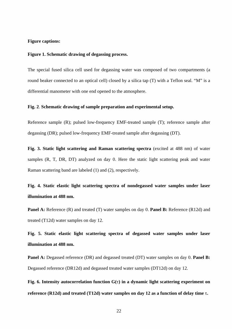
Figure captions:

Figure 1. Schematic drawing of degassing process.

The special fused silica cell used for degassing water was composed of two compartments (a

round beaker connected to an optical cell) closed by a silica tap (T) with a Teflon seal. “M” is a

differential manometer with one end opened to the atmosphere.

Fig. 2. Schematic drawing of sample preparation and experimental setup.

Reference sample (R); pulsed low-frequency EMF-treated sample (T); reference sample after

degassing (DR); pulsed low-frequency EMF-treated sample after degassing (DT).

Fig. 3. Static light scattering and Raman scattering spectra (excited at 488 nm) of water

samples (R, T, DR, DT) analyzed on day 0. Here the static light scattering peak and water

Raman scattering band are labeled (1) and (2), respectively.

Fig. 4. Static elastic light scattering spectra of nondegassed water samples under laser

illumination at 488 nm.

Panel A: Reference (R) and treated (T) water samples on day 0. Panel B: Reference (R12d) and

treated (T12d) water samples on day 12.

Fig. 5. Static elastic light scattering spectra of degassed water samples under laser

illumination at 488 nm.

Panel A: Degassed reference (DR) and degassed treated (DT) water samples on day 0. Panel B:

Degassed reference (DR12d) and degassed treated water samples (DT12d) on day 12.

Fig. 6. Intensity autocorrelation function G(τ) in a dynamic light scattering experiment on

reference (R12d) and treated (T12d) water samples on day 12 as a function of delay time τ.

23

Inset: Low τ values (25 - 15000 µs) showing the short delay time of R12d. Exponential fit of

G(τ), solid line.

24

Figures:

Figure 1:

Figure 2:

25

Figure 3:

Figure 4.

Panel A Panel B

26

Figure 5.

Panel A Panel B

Figure 6: