Effects of Random FluctuationNoise on FM and FDM/FM Reception

Item Type text; Proceedings

Authors Wachsman, R. H.; Baghdady, E. J.

Publisher International Foundation for Telemetering

Journal International Telemetering Conference Proceedings

Rights Copyright © International Foundation for Telemetering

Download date 13/06/2018 03:30:52

Link to Item http://hdl.handle.net/10150/606333

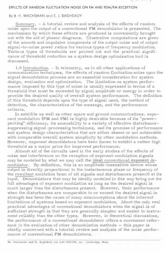
EFFECTS OF RANDOM FLυCTUATION NOISE ON FM AND FDM/FM RECEPTlON

By R. H. WACHSMAN and E. J. BAGHDADY

Summary. -A tutorial review and analysis of the effects of random noise upon the output of a conventional FM demodulator is presented. The mechanism by which these effects are produced is conveniently brought out with the aid of phasor diagrams. Illustrative computations are given of the smooth and impulsive components of the output noise and of output signal-to-noise power ratios for various types of frequency modulation. Various types of thresholds are pointed out and the practical signifi­cance of threshold reduction as a system desig_n optimization tool is discussed.

1 .01ntroduction. - In telemetry， as in all other applications of communication techniques， the effects of random fluctuation noise upon the signal demodulation process are an essential consideration for system design， evaluation and optimization. The limitation on system perfor­mance imposed by this type of noise is usually expressed in terms of a threshold that must be exceeded by signal amplitude or energy in order to provide the desired quality of overall system performance. The definition of this threshold depends upon the type of signal used， the method of detection， the characteristics of the message， and the performance criteria.

In satellite as well as other space and ground communications， expo­nent modulation (FM and PM) is highly desirable because of its "power­packing" efficiency， its amenability to a variety of effective disturbance-suppressing signal-processing techniques， 剖ld its promise of performance and system design characteristics that are either absent or not achievable with comparable overall system simplicity by other modulation methods. However， exponent demodulators have been known to exhibit a rather high threshold as a major price for improved performance.

Almost all of the circuits used in the early studies of the effects of noise and interference on the reception of exponent-modulation signals may be modeled by what we may call the.!deal conventional exponent de­modulato!'. By definition， this is an amplitude -insensitive device whose output is directly proportional to the instantaneous phase or frequency of the resultant excitation (sum of all signals and disturbances present) at its input. Demodulators that may be ideally modeled in this way bring out the full advantages of exponent modulation as long as the desired signal is much larger than the disturbances present. However， their performance when the disturbances are comparable to or exceed the desired signal in strength has been the cause of many misconceptions about the inherent limitations of systems based on exponent modulation. About the only real practical advantages of conventional demodulators when the signal is of sufficient strength is that they are generally simpler and easier to instru­ment reliably than the other types. However， in theoretical discussions， the performance of a conventional demodulator offers a convenient refer­ence in the evaluation of other demodulation methods - this paper is chiefly concerned with a tutorial review and analysis of the noise perfor­mance of conventional FM demodulators.

Mr. Wachsman and Dr. Baghdady are with ADCOM， Inc.， Cambridge， Mass.

An abstract of the effects of random noise upon the output of a con­ventional FM demodulator is presented in Section 2.0. The mechanism by which these effects are produced is conveniently brought out with the aid of phasor diagrams in Section 3.0. The smooth and impulsive components of the output noise are then treated separately in Sections 4.0 and 5.0. Illustrative computations of output signal-to-noise power ratios are pre­sented in Section 6.0 for various types of frequency modulation. The concept of "threshold" is finally explored in Section 7.0 and the practical significance of threshold reduction as a system design optimization tool is discussed.

2.0 Summary of Effects of Thermal Noise on FM Detection. - The effects of thermal-type (or smooth) noise on FM reception can be summarized as follows:

At very high S/N主坐坐呈(ratios of carrier power to total noise power) at the input to a conventional (limiter-discriminator) FM demodu­lator. the output consists of an essentially undistorted replica of the wave­form that describes the instantaneous frequency fluctuations of the input signal component. plus旦旦components of noise. The first component of noise is smooth. but non-stationary. gaussian noise (if the input noise is gaussian) with a power spectral density that varies with frequency. ω. in accordance with

qG

、.，ω .可Ed'，.、P

AI

H 、.，PI

-2.4

ω .、..

"

ω --d

，s﹒、gi

.‘主γ

••

h

Ti

qd

ω where white front-end thermal noise is assumed. and

H品.，(jω) = Overall combined RF and IF frequency response •• characteristic of the receiver (linear) stages

preceding the FM demodulator; ωif = Center frequency of Hif(jω) in rad/ sec; and

H ^ _ (jω) = The frequency response characteristic of the 且p combined lowpass filter action of the FM discriminator lowpass circuit and the baseband filter that follows the discriminator.

The second component of noise is impulsive in character and occurs with such low probability that it is usually ignored in analog communications. The probability of occurrence of this noise 泊. however. often not small enough to be ignored in digital communicati<�ns (such as PCM/FM) where averãge error-prObabilities of less than 10- 2 are a performa�ce requirement.

As the input S/N ratio is reduced. important effects set in when the input S/N ratio falls below about 10 dB. First. the output ratio of signal power to smooth noise power begins to show non-neg且gible departure from 且盟主!' dependence upon the input ratio of carrier power to total noise power. Thus. the approximation of the smooth component of output noise by gaussian statistics begins to break down rapidly. Second. the proba­bility of occurrence of the impulses rises to the point where the number of impulses occurring per unit time is sufficient for this component of noise to dominate eventually. Third. the increased number of impulses and their overwhelming tendency to point toward zero output level results in a progressively increasing depression of the output signal component by multiplying it in effect by the reduction factor 1 - e﹒ρ. where ρ= (S/N)if' Fourth. significant components of nonlinear interaction between message

waveform and noise begin to appear; and， fifth， signi紅cant distortion of the message waveform sets in.

Of all of the components of noise and distortion present in the FM baseband， impu1sive noise is the most distinguishable and becomes un­disputably the most serious at values of input S/N ratio below about 10 dB. Fortunately， because of its distinguishability， the impulse noise compo-nent can be significantly reduced in the output of a conventional Fl\且dis-criminator for all input S/N ratios down to about 7 dB. Below that， the "impu1sesll on the average occur so frequent1y， and with such increased durations， that they effectively mask significant portions of the desired message waveform.

3.0 Analytical Model and Description of FM Capture Effect With Random Fluctuation Noise. - A simple analysis can be given to

lend theoretical support for the type of performance just described. This analysis also parallels the usual type of argument employed to describe the capture effect in conventional envelope and exponent demodulators when two sinusoidal-type signals are present in the input. But， first， we set up the basic mathematical expressions that we shal1 employ throughout this paper.

3.1 Mathematical Mode1. - A general exponent-modulation signal can be described by

eexp(t) = Es sin[ωct+吵(t)] (1)

where ωc is the carrier frequency， Es is a constant， and Iþ(t) is directly proportional to the message time function g(t) for phase modu1ation and t。the time integral of g(t) for frequency modulation. It is convenient to represent the total noise present within the receiver IF passband by

n. Jt) = n (t) sin ωt + n (t) cosω t (2) 11. c. C q C V(t) sin[ωct + �(t)] (3)

where the envelope V(t)， phase �(t)， and amplitudes nc(t) and nq(t) are time functions that vary slowly (relative to cosωct) for a narrowband noise process (i. e.， a noise process whose spectrum occupies a bandwidth that constitutes a small fraction of any frequency contained in this spectrum). For a narrowband gaussian noise process of zero mean， whose spectral density function is symmetrical about ωc rad/sec， V(t) is Rayleigh dis-tributed， �(t) is uniformly distributed over 0 � � � 2霄， and nc (t) and na (t) are indepcndent gaussian processes having zero means and identical spectral density functions.

The resultant of signal and noise at the output of the IF amplifier is eif(t) = Es sin {ωct+吵(t)] + V(t) sin [ωct+￠(t}] (4)

If the signal and noise components in this sum are represented by phasors， the properties of the sum can be interpreted with the aid of phase diagrams as illustrated in Figure 1 . Figure l(a) illustrates the situation in which the total noise remains weaker than the signal (i. e.， V(t) < Es) over a time interval in which the tip of the noise phasor traces a complete rota-tion about the tip of the signal phasor. Fig叫e 1 (b) illustrates the

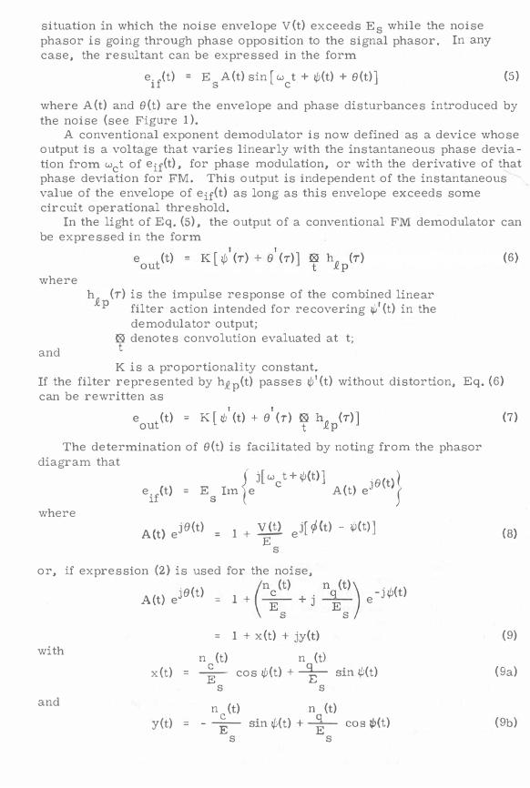
situation in which the noise envelope V(t) exceeds Es while the noise phasor is going through phase opposition to the signal phasor. In any case， the resultant can be expressed in the form

eif{t)=ESA(t)sin[ωct+吵(t)+ e(t)] (5)

where A(t) and e(t) are the envelope and phase disturbances introduced by the noise (see Fi巳rre 1 ).

A conventional exponent demodulator is now defined as a device whose output is a voltage that varies linearly with the instantaneous phase devia­tion from ωct of eif(t)， for phase modulation， or with the derivative of that phase deviation for Fl\ιThis output is independent of the instantaneous value of the envelope of eif(t) as long as this envelope exceeds some circuit operational threshold.

In the light of Eq. (5)， the output of a conventional FM demodulator can be expressed in the form

(t) = K [吵 (r) +θ (r)l t?! h n _(r) (6) 。ut ' -， -- L 'r ' " - ， ' 'J 1" 且pwhere

hn_ (r) is the impulse response of the combined linear t p filter action intended for recoveringν(t) in the demodulator output;

� denotes convolution evaluated at t; t and K is a proportionality constant.

If the filter represented by h.ep(t) passes吵I(t) without distortion， Eq. (6) can be rewritten as

e t(t)z k[沙(t) +θ (r) � ho • .. (r)] r --.e p (7)

The determination of e(t) is facilitated by noting from the phasor diagram that

、lstf‘-J、.，4L

'，.、nσ

-、EJe

、‘.，&L

(

A 可EEEEJ)

&Eiu

'，.、心U'+

&L C

ω FE.E.-』.、ZEU

e /ij1』1.、

m

γA S E

2

、圖，4L

(

PTE­-可Eae

where

州) ejθ(t) = 1 + 乎 ej[似t) -的)]s

or， if expression (2) is used for the noise， /n. (t) n (t)\

的) eJθ(t) = 1 + ( u;"一 + j U�" ) e -jlþ(t) \ E J E I \ S S /

= 1 + x(t) + jy(t) n (t) n (t) 主- cos吵(t) +令一 訕。(t)

s s

(8)

(9) with

x(t) (9a)

and y(t)

n (t) n (t) - 毛一 訕。(t)+ 告一 悶的)

s s (9b)

Thus θ(t)

where

1m .en {以t) eje的

= Im{.en[l + z(t)]} (10)

z(t) V(t) ej [�(t) -吵(t)] E (10a) S

= x(t) + jy(t) (10b) 3.2 FM Capture with Random Noise. - 1n the situation illustrated in

Figure l(a)， the tip of the noise phasor makes a complete excursion around the tip of the signal phasor without encircling the origin， O. This signifies that the instantaneous phase of the resultant undergoes no net change relative to the instantaneous phase抖。of the signal during the excursion illustrated in Figure l(a). Consequently the average frequency of the resultant of signal plus noise over the time interval required for the complete excursion in Figure 1 (a) is equal to the average (over the same time interval) of the instantaneous frequency吵(t) of the signal.

However， in Figure 1 (b)， as the instantaneous phase of the noise relative to the signal goes through a complete change of 27T radians， the instantaneous phase of the resultant undergoes the same change of 27T radians relative to the signal. Consequently， the average frequency of the resultant over the time interval required for the excursion in Figure 1 (b) is equal to the average (over the same time interval) of the instantaneous frequency of the noise. The important thing in Figure 1 (b) is not that E 門 < V(t) during part of the time interval of the complete excursion， but r品her the occurrence of the event E s < V(t) overlapped with the event �(t) -吵(t) =π土石， where ( is some small angle. If these two events do not occur together to allow the encirclement of the origin of the signal phasor， 0， the average frequency of the resultant over the complete excursion would remain exactly equal to the average of 心I(t) over the same interval.

Two extreme situations are of special interest. 1n the first， the signal is much stronger than the noise， and one can assert that Es >> V(t) almost all of the time. 1n this case， the instantaneous phase of eif(t) is closely approximated by

V(t) ωst+￠(t)，王一sin[Ø(t) - �(t)] (11) S

This shows that when the signal is much stronger than the noise， the instantaneous phase of the resultant of signal plus noise is effectively equal to the instantaneous phase of the signal with an added random phase perturbation whose peak value almost never exceeds a small fraction of a radian.

1n the second situation， the noise is much stronger than the signal， and here the instantaneous phase of eif(t) is c10sely approximated by

E ωst+心(t)+而言 叫仰) -州]

T.his shows that when Es << V(t) almost all of the time， the modulation 怡• (t) is effectively masked by the noise on the average.

(12)

A capture phenomenon thus enables the signal to suppress the noise when the signal is well above the noise. and it enables the noise to sup­press the signal when the noise is stronger. The character of the demodu­lator output is drastically changed in going from the extreme described by Eq. (11) to the extreme described by Eq. (12). As in the case of CW inter­ference. the demodulator output goes through a capture transition when the signal and the noise are of "comparable strengths." 1n this capture tran­sition region. the character of the output changes rapidly from a condition in which the desired message is dominant to one in which the noise is dominant.

A quantitative estimate of what is meant by "comparable strengths" for two such radica11y different types of signal as a sinusoid of constant amplitude and a random-f1uctuation noise process is handicapped by the fact that for the model noise processes usually assumed in theoretical studies. the noise envelope V(t) does not have a well-defined "equivalent peak value." Nevertheless. the theoretical models usually allow V(t) to range between 0 and ∞only with a probabi1ity density function that fa11s off rather rapidly toward zero after V exceeds a few times the rms value of the noise. One may thus arbitrari1y define some level that would. in the long run. not be exceeded by V more than a small percentage of the time. the exact value of this percentage depending upon what is judged tolerable for a particular application.

As an important illustration. we note that on the basis of numerous experimenta1 observations. noise of the type generated in receiver front ends has been judged variously to have an equivalent pe品value of between 3 and 4 times the rms va1ue of the noise. 缸. in search of theoretical corroboration. we model the noise by a narrowband gaussian process. we find that the probability that the noise envelope" y exceeds c times the rms value，Nrmy of the noise is given by rd/2. Thus ， for narmwband gaussian noise. V may be expected to exceed 3Nrms 1.111 percent of the time. and 4Nrms 0.034 percent of the time. If we arbitrarily specify the equivalent peak va1ue as the value which V(t) may exceed for less than 0.1 percent of the time. such a va1ue turns out to be approximately 3.7 Nrms' At this threshold.的INhf = 6.85. or about 8.4 dB. The factor that multiplies Nrms to yield the equiva1ent peak value is usually ca11ed "the peak factor" of the noise. Experimental "guesses" of the peak factor of front-end noise seem to cluster around a value of 3.7.

n

For a 叫rrowband gaussian noise process of mean squared value N;ms' the probability that the noise envelope value at any instant of time (t1• say) exceeds the signal amplitude. Es' is given by

where p (Vt1

>ES) = e-ρ

2 .___2 ρ = (S/N)if = ES /2tqrIIIS

(13)

(14)

This probability is strict1y nonzero for any finite value of ρ. Similarly. the event that the instantaneous phase difference �t - øt goes through the interval - � � I �+ -怡1 < 宵 + �t_ ....t_ I 1 '1

has a nonzero probability represented by P[π- f:三|￠t1

-hI|< 宵+ f:] ，

and given by the area between the horizontal axis and the probability density function

p.../(x) � P.I.(X)， ￠ 己 吵of

呵i4L

的V44

4，iv

，而Y

between宵- ( and宵+ f:: ，if P��X� and Pø.(X'>. ��e :�e �r?babi�ty

. de��ity f�nc-

tions of �t and靴， and �t and lbt are statistically independent. The value of f: depends upon the average value of the instantaneous frequency difference， I�' (t) _lþt (t) 1， during an excursion interval， being higher for greater values of the instantaneous frequency difference. Therefore， even for high values of ρ， there is a nonzero probability given by

e-ρP[霄，ES|￠t -h|<宵+f:] (14)

that an encirclement of the origin of the signal phasor will be experienced by the tip of the resultant of signal plus noise. But for high (S/N)丘， the angle ( must usually be a small fraction of 21T and the excess of Vt over Es can very rarely be large. Consequently， when an encirclement of 0 in Fi忍.lre 1 occurs for a large (SjN)if ， it must mostly occur in a very short time relative to a complete-excursion interval (see Figures 2 and 3). Such encirclements will be manifested by nearly abrupt phase jumps of up to 21T， which in turn correspond to impulsive instantaneous -frequency distur-bances of area up to 21T each. Instantaneous frequency ttspikestt will also result when the tip of the noise phasor sweeps slightly to the right of 0， without encircling O. Such spikes will enclose an area of up toπ(see Figures 2 and 3). An abrupt phase jump of magnitude宵will also result from zero crossings of the resultant amplitude A(t)， although these occurrences are rare.

The tt spikedtt FM disturbances just described have very characteristic behavior. The fact that the average frequency of the resultant over a complete excursion of the tip of the noise phasor must equal the average instantaneous frequency of the noise during that interval when an encircle­ment of 0 in Figure 1 occurs suggests that the frequency ttspikestt must generally point toward the average frequency of the noise， name旬，ωfAlso， since the noise phasor will turn faster relative to the signal phasor wh�n the :Iaveragett value of the instantaneous frequency difference I�‘(t) -φ. (t) I becomes higher， the probability of an encirclement while V(t) > ES is greater when the instantaneous frequency deviation of the sig­nal is near its peaks. Finally， as (SjN )if is reduced to lower and lower values， the larger excesses of V(t) over ES should become more and more probable. Consequently， the encirclements of 0 should generally cause slower phase transitions and hence less spiked frequency disturbances at the lower values of (S/N)if﹒ The increasing dwell time near the average frequency， ωc， of the noise over more and more consecutive excursion intervals at low values of (S/N)if causes increasingly significant distortion in the detected signal modulation.

The impulsive component of the FM baseband noise can be effectively reduced. The suppression techniques are worthy of brief consideration here. First. the two well-known techniques of saturation clipping and complete circuit interruption for the duration of an impu1se -- which are of signific缸lt value in combatting RF impu1sive bursts prior to demodula­tion -- are ru1ed out in the FM baseband for the following reasons:

(a) The FM baseband impulses are usually oriented toward zero voltage. and hence conventional saturation clipping is out of the question whereas circuit disruption may actually increase the severity of the "hole" introduced by the impu1se by increasing its depth and widening it.

(b) The most probable impu1ses are limited in their intensity to an area of +21T or -21T. which is comparable to or smaller than the deviation ratios of interest in most FM systems. Therefore the difference in levels between signal and impu1ses is insufficient for effective application of conventional saturation clipping or of interruption techniques.

The interesting approaches to combatting Fl\在baseband impu1ses can be termed the impulse-to-doublet conversion technique and the i旦旦且豆豆­actuated holding or clipping technique.

In the impu1se-to-doublet conversion techniqu�， each impu1se when it occurs is automa位cally converted to a doublet by a nonlinear circuit. Mathematical勻， a doublet is given by the derivative of the impulse. Therefore， since the spectral density of the impulse is f1at (a constant) over all frequencies down_ to and including 0 Hz， the power spectral density of a doublet varies with ω2 and is therefo;e zero atω= 0 and rises para­bolically as I w I is increased. This means that for a baseband signal whose spectrum extends from near zero to a few kHz， the conversion from impu1se to doublet would actually reduce the spectral density of the noise significant1y in the manner that FM demodulation actually reduces the spectral density of any input noise in going from IF to baseband.

If the desired signal，吵I (t)， 的the output of the FM discriminator is changing only slowly during the duration of the impulsive disturbance， the impulsive disturbance can be rejected by holding the output signal at the level of its instantaneous value at time immediately prior to the occur-rence of the impulse. In this w呵， continuous transmission of the base-band waveform妙1 (t) + 131 (t) is maintained呈王三三且during the times of the impulsive disturbances. At these times an impulse-actuated "hold" circuit holds the output constant.

4.0 Analysis of Smooth Noise Component. - The discussion in the preceding section highlighted the fact that the noise in the FM discrimi­nator output consists of

a Ilsmooth" compοnent -- i. e.. a component that delivers its power at a uniform rate characteristic of continuous random-f1uctuation phenomena -­and a呈型坐立component that occurs in "punches" that grow on the average more and more impulsive

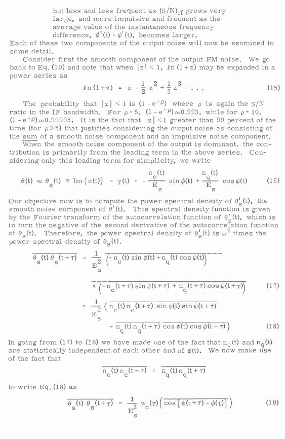
but less and less frequent as (SjN)if grows very large， and more impulsive and frequent as the average value of the instantaneous frequency difference， �'(t) -吵'(t)， becomes larger.

Each of these two components of the output noise will now be examined in some detail.

Consider first the smooth component of the output FM noise. We go back to Eq. (10) and note that when Izl < 1， _Qn (l+z) may be expanded in a

s

a CM

e .、Ar

e CM

r

e

w

o

p 1 2 1 3 _Qn (l +乞 )= z -.;;. z-+.;;.z - -2 -

3 (15)

The probability that 1 z 1 < 1 ìs (l -e-ρ) where ρis again the SjN ratio in the IF bandwidth. For ρ=5， (l-e-ρ)勾0.993， while for ρ= 10， (1 -e -P)起0.99995. It is the fact that 1 z 1 < 1 greater than 99 percent of the time (for ρ> 5) that justifies considering the output noise as consisting of the sum of a smooth noise component and an impulsive noise component.

When the smooth noise component of the output is dominant， the con­tribution is primarily from the leading term in the above series. Con-sidering only this leading term for simplicity， we write

n (t) n (t) θ(t)向θ_(t) 三 1m { z (t)} = y(t) = - � sin心(t) +� cos吵(t) (16) s '-' .---l-'-') J ' - ' E ---- .，.. ， - ， E s s

Our objective now is to compute the power spectral density of e�(t)， the smooth noise component of e' (t). This spectral density function- is given by the Fourier transform of the autocorrelation function of 札(t)， which is in turn the negative of the second derivative of the autocorre]ation function of es(t). Therefore， the power spectral density of e�(t) is w4 times the power spectral density of θs (t).

。(t)θ-(t -+ T-) = � ""7( --n-_-:-( t"'-) -si-n吵(t)+ n. (t) cos 仰)\s s E� \ c q / S

x (-n _ (t + T) sin φ(t + T) + n (t + T) cos 心(t+ T)\ (17) \ c q J = 主 { n.Jt) n，Jt + i)石布了三川(t+ T)

E - --

S + n (t) n (t + T) cos圳t) cos圳t+T)} (18)

q q ，

In going from (17) to (18) we have made use of the fact that nc(t) and nq(t) are statistically independent of each other and of 吵(t). We now make u- se of the fact that

n (t) n (t + T) = n (t) n (t + T) q q to write Eq. (18) as

θ只

ωθS(t+T) = �2 Wn(T)( 州州+T)吋(t)] ) (19)

U - E一S

where AOO w (T) = n (t) n (t+T) = n (t) n (t+T) = ( 2W(f+fJcoS(WT) df (20) n c c q q 已 C

The autocorrelation function of es(t)， and hence the power spectral density of es(T) ， depends on the statistics of the modulation through the multiplicative term

(c 叫 Iþ (t + T) - 吵圳仰州州(仇ω叫tο圳}川lin Eq. (19). For large index FM where the bandwidth required to accom­modate the modulated carrier is much larger than the bandwidth of the modulating signal 吵'(t)， the effect of the term

(c叫“t+ T) - 吵(t) ] ) on the autocorrelation function of θs (t) is small， since in this case九(T) is 口luch narrower than

(c叫心(t + T) - 吵仰州州(“的叫t)叫)門]which is equal to one for t出he small values of T t出ha叫t wnμ(T吋) is n∞ot neg斟li培gi出 bl勾y small. Since it is for large -index FM that the FM modulation method produces significant SNR improvement (above threshold) over other common forms of modulation， such as the several types of AM modulation， we shall only consider this case. Consequently，

θ (t) e (t+T) 記 -L w (7)s S _ 6 n - E - --S

and the spectral density of θ (t) is approximately s 1 2 ws(f) 笠 二三 ω 2W(f+ fc)

� s (single -sided)

5.0 Analysis of the Impulsive Noise Component of the Output. - As

(21 )

(22)

mentioned previously， impulses at the output of the FM discriminator are caused by encirclements of the origin， 0， in Figure 1 by the tip of the noise phasor turning about the tip of the signal phasor. Further illustra­tion is provided in Figure 4. In this figure two paths of the tip of the normalized signal-plus -noise vector which result in an "impulse" in e' (t) 的the output of the discriminator are shown. In path 1， e(t) increases by approximately 271"， whereas in path 2θ(t) decreases by approximately 2π. Because these paths pass c10se tοthe origin， θ(t) increases (or decreases) in an almost step-like manner. The result is a sharp narrow pulse in e' (t) which we refer to as an "impulse. 11 The phase step produced by path 1 is positive -going， which yields a frequency "impulsell of positive area approximately 271". The area under the frequency impulse corresponding to path 2 is -271".

We assume for purposes of computing the probability of occurrence of an impulse， that an impulse occurs every time thatθ(t) increases or decreases出rough an odd multiple of仇 Fol1owing Rice's formulation， we o bserve that the event 1 1θ(t) increasing through 71" between time t and t + dt" corresponds tοthe situation at time t in which the noise components x(t)

and y(t)， and their time derivatives， x' (t) and y' (t) lie simultaneously within the fol1owing ranges

-∞<xt<-li-∞<xt<∞;O〈Yt<-Yt dtJ-∞〈Yt<O (23)

1n defining this compound event， the requirement -∞<xt < -1 ensures that the signal axis is crossed on the negative �ide so that the origin is indeed cncirc1ed. The second requirement -∞<xi<∞ ref1ects the fact that it does not matter whether x(t) is increasing or

.decreasing when the signal

axis is crossed. The requirement that -∞<.Yt < 0 ensures that O(t) is increasing， whi1e the requiremen� � <yt < -yi dt e�sur�s伽t the signal axis is crossed within the time interval from t tõ t + dt. Thus， the probabi1ity of the compound event defined in Eq. (23) is

^

f-l x f∞ � J γ dt . ，.V ， ， .L dXt I<X) dx� I -

Y t u�dYt I dy� p(xt， x�， Yt' Y

�) (24) tJ _.t -L • -JtJ -Jt t""t" . t'Jt'Jt

-… _.-.r.. ，. _…

whcr可p(呵，呵，Yt'Yt) is the joint probability density function of xt'門，丸，and Yt. We shall indicate how to evaluate (24) and relate it to N�， the average v宇lue of the number of positive impulses per unit time for a given value of吭﹒ N-， the average v，alue of the number of negative impulses per upit time for a given value of吭， may be obtained from N+ by changing ψt t�..-ø� w�e�ever it a?_pear� iri \he ex♀r?SSion for Tq+-

We begin by expanding p( 呵，呵，吭，yt) in a Taylor series in Yt about yt = 0， and integrating over yt in (24). We obtain

1 一̂ t ，.r\ I t c dxt p to first order in the infinitesimal quantity dt. Next， we observe that

(a) thc probability of the occurrence of a positive-going impu1se during the time interval from t to t + dt， E q. (25)， is proportional to dt; (b) the probability of occurrence of such an impu1se in the interval from t to t + dt is much less than the probability of its non-occurrence; and (c) the probability of more than one such impulse occurring during the time interval from t to t + dt is essentially zero.

(25)

Under these conditions， the number of times that such an impulse occurs over a finite interval of time obeys poisson statistics. Specifically， if probabi1ity of the occurrence of one such impulse in the time interval from t to t + dt is denoted入+缸， the average number of such impulses per unit time， N+， is equal to入+﹒ Therefore， the quantity evaluated in Eq. (25) is precisely N+dt.

Since

九t

/Es，nqt/Es' 〈

t角s，and i

tA

are statistically independent gaussian random variables， their joint probability density function is

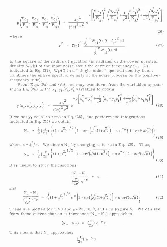
位主主可E ' E ' E ' E I s s s S I

、EEa--••

aaad

肉，仇凶

11、t』II''

，

但M S

l-2r

+

門，4.

iif-

-

他叫-nr臼1-r

+

nk凶11121，/

比-s

nf-E

J/Il--、2\抖/他問 SFEE--EE.E.-‘

e

ZJU

2-r

nv-內，心

4一

叫

自

nd(26)

where 內，心、'，何向JU'，E、一一-qL

r

fWifω(f - fc)2 df

fWIf的df

(27)

is the square of the radius of gyration (in radians) of the power spectral density Wif(f) of the input noise about the carrier frequency fc﹒As indicated in Eq. (27)， Wif(f) is a "single-sided" spectral density (i. e.， combines the entire spectral density of the noise process on the positive­frequency side).

From Eqs. (9a) and (9b)， we may transform from the variables appear­叫in Eq. (26) to伽Xt， y戶�， y� variables to obtain

r 2 2 1 I 1 . 1\2 1 I 1 1 可21. 2 -p l x;+ Yt+--Z(xt 寸的.) + 一三(yt+Xtl/!t ) I

p(Xt，X�'Yt'y�) = 一千古 e t r r I(28)

(2叫rIf we set yt equal to zero in Eq. (28)， and perform the integrations indicated in Eq. (25) we obtain

N+=i{磊) � (1 +叫/2 [1 _叮f(布可有)] - u e -p [ 1 - erf叫)] } 、

， (29) where u=心/r. We obtain N _ by changing u to -u in Eq. (29). Thus，

N_ =計划(1+u2)1/

2il m叫阿] +u e-ρ[ 1 +肘f(4)])

(30)It is useful to study the functions

+一ρ

N一 .e

Nm-FUFm

= u (31)

and +-P

N一­-e

+一)

N-一兮

LHU2)1/

2eρ[1 - erf(�(l+u2) )] +u erf(叫 (32)

These are plotted for u> 0 and ρ= 25， 16， 9， and 4 in Figure 5. We can see from these curves that as u increases (N_ +N+) approaches

的“- N+) = (工) e-ρu c，'ff

This means that N _ approaches

(之) e-Pu c，'ff

and N+ approaches zero as u increases (u > 0). (The roles of N+ and N_ are interchanged when u<O.) The polarities of the impulses are pre­dominantly opposite to the polarity of the modulation. This net unbalance in the number of positive and negative-going impulses as a function of the modulation，叫， results in a modulation depression effect in which the average or expectation of吵， + e' (averaged over the noise) is {1 - e-ρ)功，However， since (1 - e圍內is approximately 0.993 for ρ= 5， this modulation depression effect is negligible for the range of input signal-to-noise power ratio，ρ， for which our model of the discriminator output noise is valid.

From the assumption that the impulses obey Poisson statistics and have areas of土2霄， the power spectral density of the impulse component of the noise at the output of the discriminator at zero frequency may be shown to be (single-sided)

一+

-N

一+

-N

q品π

QU

nU

VE-­W (33)

where the average is over the modulation. rf the impulses were truly ideal (of infinite缸nplitude and zero duration) the power spectral density Wr{f) would extend out to infinite frequency. However， since the impulses are not ideal， the power density spectrum of the impulse component of the noise at the output of the discriminator will fall off at higher frequencies. At lower frequencies， and， in particular， over the bandwidth of the modu­lation， WT{f) is assumed to be constant as a function of frequency and equal to Wr{O). - We indicate how the average over the modulation in (N_ +N+) may be computed for several types of modulation signals in the next section.

6.0 Some Examples of SNR Computations for Various Modulating 旦旦且呈. - We shall consider three types of modulating signals: (1) a sinusoidal modulating signal; (2) a gaussian distributed modulating signal; and (3) a modulating signal consisting of n sinusoidal

tones which may in turn be FM (or PM) modulated. For simplicity of computation we assume a rectangular IF spectrum of

bandwidth Bif = 2恥 ，where ω is the highest frequency in Iþ' (t). and k is a constant cEOsen tFensure thEthe IF bandwidth is sufficiently wide to pass the FM-modulated carrier without significant distοrtion. rn selecting k we mak e use of Carson's bandwidth rule that

Bif = 2 k.ωm = 2{t..ω+ωm}radians/sec (34)

where t.ω is the maximum frequency deviation. For such an IF spectrum，the power density spectrum W(f+fc) is (for

ω<kωm)

W川 = 石)/(主) = :三t)/ (平) (35)

so that 1 2 一2

W (f)空一τω 2W{f +f ) = 一 w一

E 2 - - .. ， - . -c ρ kωm S

2 7r ω (36) ρωm偕 + 1)

The noise power from ω= 0 toω=ωm resulting from the smooth noise component of the output is

2 fωm ___ ，.，dω 1 ， 1 ω

= I 心 W (f)一 = (一)一 一一一4 2何 2ρ 3 /但+ 1 \ W I 、 紅l '

1) Sinusoida1 modu1ating signa1: Here心'(t) is

(37)

吵 (t) = t:.ω cosω t = mω cosω t (38) 口1 口1

where m = t:.ω/ωm is known as the modu1ation index. rn this case Eq. (37) becomes

N S

2 1 1 ωm

(2ρ) 3 (m + 1) (39)

The radius of gyration， r， of the rectan恩ùar spectrum is kω (m + 1)ω m 口1r = Jτ J吉

so that u lS t max l/!max Aω m，J3 u

口1ax r r m+1

(40)

(41 )

To compute (N_ +N+) we first note that for u greater than about 0.4 (for ρ>4) (see Fi巳lre 5)

N+但O and 札記.$- e-ρ 4已 7r

(42a)

For u $ 0.4，

N 目。 and N 戶~二生-e-ρ� 27r (42b)

Since I u I is greater than 0.4 approximately 85 percent of the time for the case of a sinusoida1 modu1ating signa1 with umax何./3' (m is assumed 1arge)， and since most of the impu1ses occur near the peaks of松I(t) (near u = umax>' we sha11 use the above approximations for all u in computing (N _ +N+). We obtain

京市72(4)平 (43)

Therefore Wr(f) is

Wr(f) = 8π2頁_+N+) = 8mωm e ρ (44)

The noise power from these impu1ses from ω= 0 toω=ωm is

以}_N T = WT(f) ，.;之1 "1'. / 2π ρ

e

2m

ω

m

4一π (45)

The total output noise power from ω = 0 toω =ωm is 2 ωm r. 24 . ， -。可N_ = N_ + N T = /<'1_\');:'. ，\ f1 + -:.� m(m +1) ρe 1'1 I (2ρ) 3 (m + 1) L . .

1r U� \�.. • • I l' V J (46)

1 2 2 The output siglumtomnoise power ratio is therefore {with SO =互mωm)

s 。-

NO3ρm2(m+1)

24 . ， -0 (1 +7m{m+1) ρe 1') (47)

lS This is plotted for m = 5 and ρ> 5(7b) in Figure 6. A1so p10tted in Figure 6

24 . ， -0 7IIl(IIl +1)ρe l' for m = 5 and ρ> 5.

2) Gaussian modulating signa1: Here 吵(t) is from a乞ero mean gaussian process and has a maximum frequency ofω radians/sec. We choose the

自1�.-�.__.- I

variance of ￠『(t) so that the output signal power is the same as for the case of the sinusoidal modu1ating signa1.

o

ed

--q函、'，&BLV

，s﹒、爪的? 2 σ . 吵 ， (48)

We assume that the peak factor (ratio of peak power to average power) of the gaussian modulation is 10 dB. so that the maximum frequency devia­tion is J昂σ怡，. The constant k is therefore

k = (../5 m + 1) (49) The radius of gyration. r. is

kω 口1r =

Jτ and u is 口lax

心maxu = 口lax r

的m+1) ωm (50) 信J言

2至alb' r = J3估計) (51)

(N _ +N+)

We compute (N_+N+) by averaging (N_+N+) statistically.

where p(lþ) d心 is given by

f∞(N -+N+) p(4) d妙，

-0。

(52)

. 2 ，_ 2 ， 1 -妙' "/2σ山f

p(吵) d吵 = τ手于一e 'f' 代/，c，1rυ .v 一 .. 吵，

2 ， 2 and where a=σø' /r" and u =怡，/r.

l-5

(53)

百六而 = {i}e-ρ f∞ 1 e-U2/叫u erf(uJp) 1-' \2甘 心J27ra '- I

+吋(“1+叭川川+糾川J吋u♂凸叫IPλ斤伊2訂叩)戶1/2 eP [卜1卜川…且→叫叫e盯叮叫rFor la叮rg酹e ρ we may make use of the asympt切ot位ic expansion

川1叫1 - erf(石古)]=豆豆 11拉克+. . .1

(54)

(55)

If we retain only the leading term in Eq. (55) and integrate the first half of Eq. (56) by parts we obtain

前1站立已) e-ρ泣起丘y /2 = iJ5m+1) (2旦) e -P(立全丘 1/21'"' '2付 1 宵ρ / J言 2宵 \宵ρ/

2 . 2 _ 2.. .=-For m = 5. 2a = 2σ� ， /r"'= 3m"'/(J5 m+1)=0.504. Therefore Wr(f) is

(56)

W1(f) = 8宵2 (N_ +N+) = 但 ($ m + 1) W___ e - P 俱2主吋/2(57) J3 ，.v - --- - ， -m - \刊!

The noise power from these impulses from ω= 0 toω=ωm is

，..，..， ') _ ') _，，/1 + ')"，，，\1/2 N_ = W_(f)至二= ;:. (J5 m + 1)ω - e 1-'(.二一二三叫 ，1 i �7r J3 m \ 7rρ/

The total output noise power from ω= 0 toω=ωm is

2 N 叫 + N_ = ωm l 1+4J言(j5m+ 1)2ρJI江三至.ey/2 1

1 (2ρ) 3(Jτm + 1 L '" A'V V \'V V ."". J.. ' " 1 1-''''' \ 宵ρ / J 1 2 2 The output sigldato-noise power ratio is therefore (SO=互mωm)

(主) = 1 + 4 .5 1.;ρ

Nm+1)L Nol - 1 + 4J言 (j5 m+ 1)2 ρe哨 位瑩的1/2

亨 、7rρr

(58)

(59)

(60)

This �s plotted for m = 5 and ρ� 5 (7 dB) in Figure 7. The additional term 6/5m乙in the denominator of (8o/No) in Figure 7 is the first-order correction obtained by evaluatiñg

in Eq. (19). "\月!e also plot (c叫心T) -的(t)1

4J言(j5m+ 1)2 ρe-ρι益 的1/2 for m=5 and ρ>5 \ 7rρ / in Figure 7.

3) Multi tone case: Here吵(t) consists of the sum of n sinusoidal tones which may in turn be FM (or PM) modulated.

n 砂(t) = ) /::，.ω n cos(ω' n t +札(t).Q=1 晶 晶 晶 (61 )

With n � 4， and the /::，.ωk equal (or approximately equa日 ， 吵 (t) is approxi­mately gaussian amplitude distributed with variance σ去， given by

一一一一一- n �

'...2 1 \' 2 1 2 2 σ.1， ' = 心(t)- = 一 ) /::，.ω = 一φ L.， 且 2γ 且=1 (62) Here ωm is the highest modulating frequency in松(t)， and m is defined by Eq. (62).

Making use of the results of the previous case， the total output noise power density spectrum over the bandwidth of the modulation is

2 I _/w \2 / _ \ ， /<>1 W (f) 222 ω 11 +土的m+1)2(、rpe-ρ江三叫1/21 (63) (2ρ)的m+ 1 )ω: 1 λ {τρ e

lπρ Î I th The signal power at the output of the且 tone recovery filter whose noise

bandwidth is B且radians/sec is 1 . . .2 = 一(/::，.ω )- (64) 且 2 且

Assuming that the spectrum W。(f) is essentially constant and equal to W，...(fo ) over the tone filter noise bandwidth B o ， the signal-to-noise power ra1io� at the output of the kth tone filter is �

/W \2/1ω\ //::，.ω.\' (或

Iρ川問問{一) 、

1\勻/ \.o_e / \ Wm/

N I rφ 呵。 I _/W \- / . _ \l /2 I X b + !. (，)5 m + 1) 2(又)ρJ{i孕的1-1l 吋 V \ -k / \ .. r- / I

(65)

- .. . . .. ___ :. .. . th This signal-to-noise ratio may be used as the input SNR to the _e _u tone FM discriminator (or PM demodulator) in order to determine its output SNR. For Bo <<ω the statistics of the noise into the _eth tone Fl\在dis-X --Wm， criminator (or PM demodulator) may be assumed gaussian and the output SNR of the _eth tone FM discriminator may be computed in the manner indicated in this paper.

7.0 Types and Significance of Noise Threshold. - The concept of a "threshold" implies

(a) a recognition of the existence of more than one adjoining mode of behavior， grade of performance or state of affairs， and (b) that a point can be defined marking， with specified approximation， the completion of a transition from one set of conditions to another.

Thus， a quantitative analysis of the noise threshold of a demodulator requires a precise definition of the conditions ushered by the "threshold. 1 1

A few such conditions will now be considered， and the corresponding thresholds estimated. This discussion should illustrate the degree of arbitrariness that may generally surround the definition of a threshold， and the dependence of the definition upon the special interests of the 11 definer. 1 1

7.1 Threshold of Improvement Over Linear Modulation. - This threshold is of interest because it marks the level of IF S/N ratio above which the baseband S/N ratio of the exponent-modulation receiver would exceed the baseba吋 S/N ratio of a linear -modulation system， under comparable conditions of IF signal and noise， with wideband exponent­modulation operation. At this threshold， we speak of the signal and the noise as being of "comparable" strengths or of "equivalent" amplitudes.

A quantitative estimate of about 8 dB was given in Section 3.2 for this threshold.

7.2 Threshold of Linear Output vs. Input S/N . - This threshold is of special interest in the analysis of the noise performance of conventional exponent demodulators because:

(a) in Fl\丘， this is the threshold of achieving the "full" improvement attributable tοwideband operation; (b) above this threshold the demodulator treats the sum of signal and noise in an essentially "linear" manner except for the occasional impulse that may occur in the output， which in a sense corresponds to occasional impulse-noise-like behavior of the thermal noise in the IF passband; and (c) the assumption of operation above this threshold provides great analytical convenience in the analysis of frequency-compressive feedback and phase-locked loop demodulators.

It can be shown that practical estimates for this threshold are: 的jN )if = 7 dB for phase demodulators

= 10 dB for conventional FM demodulator. These estimates are based on a 10 percent departure from linear behavior.

One frequently encounters published theoretical and experimental curves in which demodulator output SjN power ratio is plotted as a func­tion of input SjN ratio for values of the latter down to well below the threshold of linear dependence. Such data must be treated with the greatest caution because the normal interpretations of the significance of the output signal-to-noise power ratio over the linear portion of the curve may break down completely below the threshold of linearity. Specifically， in FM demodulation， it is important to realize that when the ìmpulsive component of the output noìse does ìndeed become sìgnificant (ì. e. ， the probabìlìty of havìng an ìmpulse ìs not too low)， the whole matter of how to treat the various output noìse components in relation to the desired baseband signal must be reconsidered. Specifically， the sìgnìficance of "total noìse power" as obtained by adding the average powers of the various noise components is defìnitely questionable . The impulsive component of the noise affects the usefulness of the output signal in a manner that is quite distinct from that of the other noise

components. N watts of average impulsive power cannot be equated to (or otherwise treated in the same manner as) N watts of average power of random fluctuation noise or N watts of average power of nonlinear distοr­tion components. Therefore the meaning of an S/N ratio in which the average noise power is taken as the su口1 of the average powers in the impu1sive and other components of output noise is doubtful， and it definitely does not reflect the same performance quality or characteris-tics as 叩 equal value of S/N ratio when only random fluctuation noise. or only impu1sive noise. is present.

The various disturbances in the noise capture transition region and below affect the baseband signal in characteristically distinct ways. and therefore their powers cannot be considered of equivalent significance and additive with equal weightin��.

7.3 Threshold of "Acceptable Performance''. - In many applications still another threshold is usually specified which may， in general. fall anywhere relative to the other thresholds， but is often chosen well above these thresholds in the region of high S/N performance. For convenience such a threshold may be termed the threshold of acceptable performance. Such a threshold is usually dictated by a specification of a maximum tοlerable error probability or the lowest tolerable quality of received audio or video information.

In this connection， it is interesting to point out that the main advantage usually sought in wideband FM is that. for most current communications， it is perhaps the simplest system (involving special signal design) for lowering the threshold for achieving a desired high quality of performance. But， as we noted earlier， the conventional (or Armstrong-type) FM tech­nique. provides the reduction in the " high-performance" threshold to a degree that is severely limited by a corresponding rise in the " threshold of full improvement. " The high S/N performance improves with increased frequency deviation until the associated increase in required receiver IF bandwidth raises the threshold of fu11 improvement to the level of the high-performance threshold. Techniques for holding the threshold of full improvement essentially fixed at the same time that the high S/N perfor­mance is raised， and tech叫ques for achieving better high S/N performance with a lower attendant threshold of fUll improvement are feasible and highly desirable.

7 .4 Bearing of Threshold Reduction on Telemetry System Desigr1. -The concept of threshold reduction is usually understood to mean an extension of the region in which output S/N is related linear句 to input S/N below the point at which this type of relationship breaks down for a con-ventional FM demodu1ator. Otherwise， the high S/N performance is not affected. One might therefore inquire what good this type of performance extension is when the threshold of acceptable performance falls well above the nonlinear parts of the output-input S/N characteristic. The answer is that this threshold reduction capability may be used in combination with an increase in the frequency deviation at the transmitter in order tο reflect some of this improvement dìrectly into the high S/N performance with or without some saving of transmitter power. For example. with the aid of a threshold reduction technique. we may trade increased signal bandwidth for a reduction in transmitter power without affecting the threshold of acceptable performance (which is assumed to fall at or above the

threshold of full improvement). When reducing transmitter power， one must， of course， guard against increasing the system sensitivity to dis-turbances other than additive random-fluctuation noise. Alternately， with the aid of a threshold reduction technique， we may trade increased signal bandwidth for improvement of the high SjN performance keeping fixed the transmitter power and receiver threshold of linear output-input SjN characteristic. The extent to which such achievements may be realized depends， however， upon the threshold-reduction technique employed at the receiver.

Reference 1 - Rice， S. 0. ， "Noise in FM Receivers， " in Time Series

企些垃是呈， M. Rosenblatt， Editor， John Wiley and Sons， Inc. ， New York， N. Y. ， 1963， Chapter 25， pp. 395 - 422.

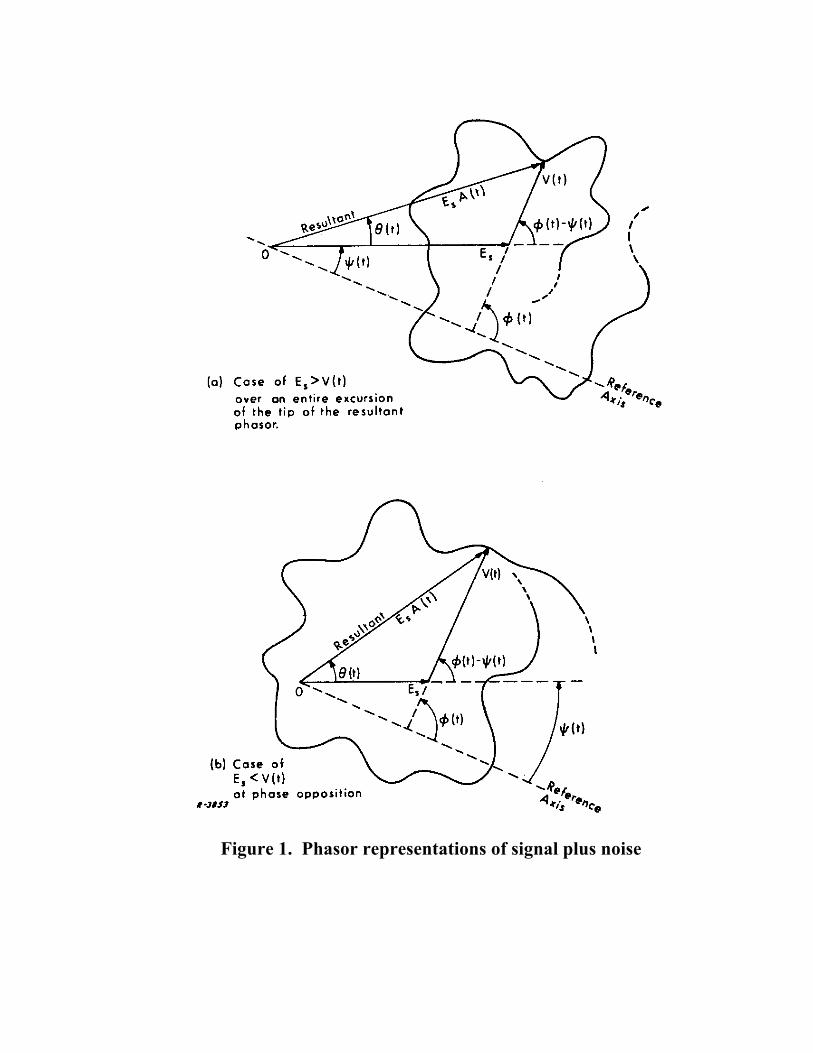
Figure 1. Phasor representations of signal plus noise

Figure 2.

Figure 3. Waveforms of 2(t) and 2'(t) for Paths 1 and 2 of Fig. 2.

Figure 4. Normalized Signal Plus Noise Vector Diagram IllustratingHow Impulses Are Produced

Figure 5.

Figure 6. (So/ No) for a sinusoidal modulating signal with modulationindex = 5.

Figure 7. (So/No) for a Gaussian modulating signal