UNIVERSIDADE DE LISBOA

FACULDADE DE CIÊNCIAS

DEPARTAMENTO DE BIOLOGIA ANIMAL

Effects of seasonality on the responses of Neotropical bats to

local- and landscape-scale attributes in a fragmented landscape

Mestrado em Biologia da Conservação

2015

Dissertação orientada por:

Dr. Christoph Friedrich Johannes Meyer

José Ricardo Teixeira Rocha

Diogo Filipe Angelo Ferreira

2

3

Agradecimentos

Esta investigação foi financiada pela Fundação para a Ciência e a Tecnologia (FCT) através do projeto “Temporal

dynamics of the impacts of forest fragmentation on Neotropical bat assemblages”.

Ao Christoph Meyer, por ter ser sido um orientador espetacular e ter estado lá sempre que eu tinha alguma dúvida

ou problema. E a cima de tudo por ter confiado em mim e ter-me dado a oportunidade de ir à Amazónia.

Ao Ricardo Rocha, por me ter ajudado não só na elaboração desta tese mas por ter feito um papel magnífico

enquanto meu orientador. Mas acima de tudo por ter sido um grande companheiro de campo e de trabalho, e ter

tornado a estadia na Amazónia ainda mais magnífica.

Ao Adrià López-Baucells, por todo o apoio e ajuda que me deu ao longo deste ano, que foi muito mais do que eu

alguma vez esperaria. E como é lógico, por todos os momentos e discussões que tornaram as recordações da

Amazónia ainda mais espetaculares.

Ao pessoal, por me ajudarem a superar todas as frustrações que ocorreram ao longo desta etapa e estarem lá sempre

presentes para ir beber uma jola. Vocês são awesome. Em especial à Marta Nabais, que para além de ter estado lá

sempre, foi uma ajuda enorme na redação desta tese e um exemplo ao longo destes anos.

Aos meus pais, porque sem eles nada disto seria possível e não sei o que seria de mim sem a ajuda deles. Espero

que todos os sacríficos que fizeram tenham valido a pena, e independentemente do que conseguir na minha vida,

estarei sempre grato e serão sempre o meu maior exemplo de vida.

“If I have seen further, it is by standing on the shoulders of giants”

Isaac Newton

4

5

Index

Resumo ......................................................................................................................................................................7

Abstract .................................................................................................................................................................. 10

Introduction ........................................................................................................................................................... 11

Methods .................................................................................................................................................................. 15

Study Area ........................................................................................................................................................... 15

Experimental design ............................................................................................................................................ 15

Bat sampling ........................................................................................................................................................ 17

Environmental characteristics ............................................................................................................................. 17

Local-scale variables ....................................................................................................................................... 17

Landscape structure ........................................................................................................................................ 18

Data Analysis ...................................................................................................................................................... 18

Influence of season and habitat type on bat abundance patterns .................................................................... 18

Relative importance of local and landscape-scale predictors of bat abundance ............................................ 19

Results ..................................................................................................................................................................... 20

Influence of season and habitat type on bat abundance patterns ......................................................................... 20

Relative importance of local and landscape-scale predictors of bat abundance .................................................. 21

Discussion ............................................................................................................................................................... 26

Influence of season and habitat type on bat abundance patterns ......................................................................... 26

Effects of seasonality on bat abundance responses to local and landscape-scale predictors ............................... 27

Frugivore ensemble ......................................................................................................................................... 28

Animalivore ensemble ..................................................................................................................................... 29

Conclusions ............................................................................................................................................................ 31

References .............................................................................................................................................................. 32

Supplementary Materials ..................................................................................................................................... 38

6

7

Resumo

Nos trópicos, o acréscimo da desflorestação está a originar paisagens compostas por fragmentos de pequenas

dimensões de floresta natural (floresta primária) circundada por uma matriz de habitat modificado. A sazonalidade

nos trópicos é marcada por diferenças na precipitação, sendo que estas diferenças entre a estação seca e húmida

podem levar a alterações na produtividade primária, no crescimento e nos padrões de frutificação e floração de

algumas plantas tropicais. Estas mudanças na produção primária podem provocar oscilações na disponibilidade de

recursos, afetando a presença e a abundância não apenas de espécies frugívoras e nectarívoras, mas também de

espécies insectívoras. Quando a sazonalidade atua conjuntamente com a fragmentação, os impactos da última sobre

a biodiversidade podem ser agravados. Isto acontece porque as flutuações naturais na disponibilidade de recursos

podem ser alteradas tanto por diferenças nas condições microclimáticas nas bordas dos fragmentos como pela matriz

de habitat modificada ação humana. Adicionalmente, a fragmentação pode ainda impedir migrações sazonais e

diminuir o acesso a recursos essenciais, impedindo o acesso a recursos (alimento e abrigo) necessários durante e.g.

as épocas de reprodução. Os morcegos são considerados um grupo de grande interesse para o estudo dos impactos

da fragmentação nos Neotrópicos, este facto deve-se à sua grande abundância, riqueza específica, diversidade

ecológica, mobilidade e importância como bioindicadores. O voo dota os morcegos de uma maior capacidade de

deslocação em paisagens fragmentadas do que outros grupos faunísticos menos móveis. No entanto, devido a

diferenças nas características biológicas e ecológicas entre espécies, as respostas a estas perturbações são muito

variáveis. Estas diferenças interespecíficas, i.e. nos hábitos alimentares, são afetadas pela sazonalidade,

influenciando a forma como diferentes espécies respondem às características de composição e configuração da

paisagem e à estrutura da vegetação ao nível local. Apesar de muitos estudos já terem averiguado os impactos da

fragmentação ao nível da população e da comunidade nos Neotrópicos, poucos foram realizados ao longo de grandes

períodos, e consequentemente as variações sazonais nas respostas dos morcegos foram raramente consideradas.

Neste estudo avaliámos como diferentes espécies de morcegos respondem à sazonalidade numa paisagem

caracterizada por fragmentos de diferentes tamanhos e circundados por uma matriz de floresta secundária em

diferentes estágios sucessionais. Recorrendo a dados de dois anos de capturas, averiguámos como é que padrões

gerais da abundância de diferentes espécies de morcegos variam entre a estação seca e húmida nos fragmentos, na

matriz de floresta secundária e em áreas de floresta contínua. Para além disto, analisámos a influência da estrutura

da vegetação (métrica de escala local), e das métricas da composição e configuração da paisagem (para cinco escalas

espaciais) na abundância de oito espécies de morcegos. Testámos também se a importância das métricas variava

entre as estações.

O estudo foi realizado no Projeto Dinâmica Biológica de Fragmentos Florestais (PDBFF), Amazónia Central,

Brasil. Os morcegos foram capturados durante dois anos em oito fragmentos e nove áreas de controlo. Em cada

categoria de habitat foram amostrado o interior, a borda e a matriz. As métricas da paisagem foram obtidas para a

8

área do PDBFF, tendo sido utilizados buffers de cinco tamanhos diferentes (250, 500, 750, 1000, 1500m de raio)

em cada um dos 39 locais de amostragem. Para cada uma dos buffers foram calculadas quatro métricas de

composição: cobertura da floresta primária, coberturas da floresta secundária – estágio inicial (6 < idade) estágio

intermédio (6 ≥ idade < 16) e estágio avançado (idade ≥ 16). Adicionalmente, foram calculadas também quatro

métricas de configuração: densidade de bordas, densidade de fragmentos, distancia ao vizinho mais próximo e

índice médio de forma. Modelos lineares generalizados mistos foram usados para testar as diferenças na abundância

de cada espécie entre as estações (seca e húmida) e entre os tipos de habitat (interior, borda e matriz). Por último,

para determinar a importância de cada métrica em cada estação usámos uma Partição Hierárquica.

Os padrões da abundância variaram com a espécie e o tipo de habitat, e foram observadas diferenças entre as

estações em todos os tipos de habitat. As relações entre a abundância das espécies com a estrutura da vegetação

local e com as métricas da paisagem foram dependentes da estação e da escala. As métricas da composição foram,

no geral, mais influentes na estação seca, enquanto a estrutura da vegetação local e as métricas da configuração

foram por sua vez mais influentes na estação húmida. A maneira como as diferentes espécies responderam a estas

métricas variou entre as espécies frugívoras e as espécies animalívoras. Na estação seca, os morcegos frugívoros

responderam mais às métricas da composição enquanto na estação húmida a escala local e as métricas da

configuração foram mais marcantes. Os morcegos animalívoros demonstraram padrões similares entre as duas

estações, respondendo ao mesmo grupo de métricas na estação seca e húmida. Devido a resultados bastante

específicos para cada escala e para cada espécie, padrões gerais em relação às métricas mais importantes em cada

escala espacial foram difíceis de identificar. No entanto, as métricas de composição e configuração foram selecionas

em todas as escalas espaciais para as duas ensembles sem padrões discerníveis, mas a estrutura da vegetação mostrou

padrões mais consistentes entre as escalas espaciais para as espécies frugívoras. No geral, a floresta secundária

estava associada positivamente com a abundância dos frugívoros enquanto para as espécies animalívoras esta estava

associada negativamente, sendo que este padrão se destacou sobretudo na floresta secundária de estágio sucessional

avançado.

As taxas de captura variaram entre as estações, sendo que algumas espécies demonstraram padrões sazonais

evidentes. Estas diferenças de abundância ocorreram sobretudo nos habitats modificados (fragmentos, bordas e

matriz), e estão provavelmente relacionadas com diferenças fenológicas nos períodos de floração e frutificação na

matriz de floresta secundária. A associação positiva com a floresta secundária e a variabilidade nas respostas à

fragmentação dos morcegos frugívoros parece suportar esta hipótese. Os morcegos animalivorous demonstraram

padrões similares entre a estação seca e húmida, indicando que para esta ensemble, a sazonalidade e

consequentemente a variabilidade na disponibilidade dos recursos pode não ser tão importante quanto para os

morcegos frugívoros.

9

É ainda importante desenvolver estudos de forma a poder perceber como cada espécie explora o habitat e como a

respetiva dieta é afetada pela fragmentação e pela sazonalidade, especialmente quando efeitos sinergéticos entre a

fragmentação e sazonalidade podem desencadear efeitos ao nível das interações planta-morcego, diretamente

através da dispersão de sementes e polinização e indiretamente através do controlo de artrópodes herbívoros. Em

paisagens fragmentadas, os morcegos beneficiarão de ações que visem promover a regeneração da floresta

secundária, de forma a minimizar o contraste entre fragmentos e a matriz. No entanto, a preservação das florestas

primárias e contínuas deve ser priorizada, de modo a garantir condições de habitat adequadas não só para as espécies

frugívoras mas também para as espécies animalívoras. Por último, a sazonalidade deve também ser consideradas

nas ações de conservação para garantir que os morcegos possuam os recursos necessários durante a época não

reprodutiva e reprodutiva, sendo a segunda, a época que exige uma maior necessidade de recursos alimentares por

parte deste grupo taxonómico.

Palavras-chave: morcegos, fragmentação, sazonalidade, estrutura da paisagem, estrutura da vegetação local.

10

Abstract

Changes in plant production can cause oscillations in resource availability, affecting the presence and abundance

not only of frugivorous and nectarivorous bats, but of insectivorous bats. When seasonality is associate with

fragmentation, it can exacerbate the impacts of the latter. We evaluate how different bat species respond to

seasonality in a fragmented landscape characterized by different-sized fragments of primary forest surrounded by a

matrix comprised of secondary forest in different successional stages. Based on two years of capture data, we

assessed how general patterns of different bat species abundance changed between the wet and dry seasons in forest

fragments, secondary forest sites, and continuous forest controls. Measurements of landscape characteristics were

obtained for BDFFP landscape and posteriorly general linear mixed-effects models to examine the relative effects

of local vegetation characteristics and landscape-scale metrics in shaping bat abundance patterns. Relationships

between species abundances and local vegetation structure and landscape characteristics were both season-specific

and scale-dependent. The way that species responded to these metrics varied between frugivorous and

animalivorous species. In the dry season, frugivores responded more to compositional metrics whereas during the

wet season local and configurational metrics were more important. Animalivorous species showed similar patterns

in both seasons, responding to the same group metrics in the wet and dry season. These suggest that for animalivores,

seasonality and consequently the variability in resource availability may not play such an important role as it does

for frugivores. Differences in responses occurred probably due the differences in the chronology of flowering and

fruiting events between primary forests and secondary forest matrix, which affected the dietary habitats of bats in

fragmented landscape. Management actions should promote the secondary forest regrowth and consequently

minimize the fragment and matrix contrast in order to maintain and improve habitat quality for bats, although

measures should prioritize primary forests conservation to preserve both frugivores and animalivores. Finally,

seasonality should be considered in management actions to guarantee that bats have the necessary resources during

non-breeding and breeding seasons.

Key-words: bats, fragmentation, seasonality, landscape structure, local vegetation structure.

11

Introduction

Tropical forests are the most diverse biome on the planet, harbouring more than 60% of all known plant and animal

species (Bradshaw et al. 2008). This is even though they only represent about 7% of the Earth’s terrestrial surface

(Bradshaw et al. 2008). Despite the significant importance of these ecosystems, they have been subjected to strong

anthropogenic pressures in the past decades, threatening the long-term stability of tropical forest biota (Bradshaw

et al. 2008; Laurance et al. 2014). The rapid loss of primary forests and the consequent habitat fragmentation are

among the greatest threats to topical biodiversity (Gibson et al. 2011; Laurance et al. 2011).

In the Amazon, increasing deforestation for cattle ranching, agriculture and logging (Asner et al. 2005; Fearnside

2001; Laurance et al. 2011; Laurance et al. 2014), is leading to the formation of landscapes composed by small

fragments of natural forest surrounded by a matrix of modified habitat (Laurance et al. 2011). Numerous studies

over the last years have shown the strong and negative impacts of forest fragmentation on animal populations in the

Amazon basin (e.g. Benchimol & Peres 2015; Figueira et al. 2015; Laurance et al. 2011) and elsewhere across the

tropics (e.g. Benchimol & Peres 2013; Bregman et al. 2014; Ewers & Didham 2006; Meyer et al. in press). The

negative impacts of fragmentation are not only associated with the consequences of deforestation per se, but also,

directly or indirectly, with a series of other disturbances. The isolation of wildlife populations due to a decrease in

connectivity between patches of suitable habitat (Quesada et al. 2004; Struebig et al. 2008) can cause the disruption

of natural movement and gene flow (Laurance et al. 2004). Generalist or exotic species that are better adapted to

fragmentation and disturbance (Goosem 1997) can occupy the niches of more specialized species, replacing them

across the landscape. Fragmentation can also cause alterations in abiotic conditions (e.g. strong winds and higher

temperatures) at the border of fragments (Ewers & Banks-Leite 2013; Laurance et al. 2002), causing edge effects

(e.g. lower relative humidity and tree mortality) that can extend up to 2 km into continuous forest (Watson et al.

2004). In addition, the increase in accessibility to humans can lead to increases in hunting and exploitation of

tropical fauna, exacerbating the consequences of fragmentation (Dirzo et al. 2014; Peres 2001). These factors

combined lead to tropical forest remnants that only contain a small portion of the original biodiversity and

communities that often differ markedly in terms of species abundance, richness and evenness from those of areas

of continuous forests (Ewers & Didham 2006; Ferraz et al. 2003).

Throughout the tropics, high rates of deforestation have drastically increased the number of old-growth tropical

forest (primary forest) patches surrounded by an anthropogenically modified matrix, such as second-growth forests,

agricultural fields, plantation forests and pastures (Melo et al. 2013). These modified matrices can act as a hostile

environment and as a selective filter, influencing the connectivity between remnant forest patches (Gascon et al.

1999). However, it has been shown that anthropogenically modified landscapes are not completely inhospitable

habitats and depending on the type of matrix and on the ecological traits of species, they can be crucial for the

survival of numerous animal species (Cisneros et al. 2015; Kupfer et al. 2006; Mendenhall et al. 2014; Watson et

12

al. 2004). Globally, tropical secondary forests represent one-sixth of all primary forest that was cut during the 1990s

(Wright 2005) and an estimated 20% of all the deforested area in the Brazilian Amazon has regenerated to some

type of secondary forest (SF) (Bentos et al. 2013). The structural similarities between SF and primary forest

(Ferreira & Prance 1999), which determine the importance of SF in terms of resources for foraging, nesting and

protection for an array of animal taxa, makes it important to take into account how SF affect the community

dynamics in fragmented landscapes. The structure and composition of SF is dependent on its age, i.e. successional

stage. In terms of floristic composition a SF will only resemble old-growth forests after decades or even centuries

(Guariguata & Ostertag 2001), and plant species turnover will be different depending on land-use history (Bentos

et al. 2013). Therefore, it is necessary to not only analyse species responses to SF as a whole, but also to assess how

they vary according to its structural and compositional characteristics, successional stage, and landscape context.

Bats (Chiroptera) are the second most diverse group of mammals with over 1300 recognized species (Fenton &

Simmons 2015), only exceeded by rodents (Kalko 1998). They reach their highest richness in the Neotropics (Kalko

1998; Patterson et al. 2003), where they are known to provide key ecosystem services (Kunz et al. 2011). The

Phyllostomidae is one of the richest and most diverse mammalian families in this region, of broad dietary scope

that ranges from fruits, pollen, leaves, insects and small vertebrates, to blood (Kalko 1998). Through seed dispersal,

pollination, regulation of small vertebrate and invertebrate populations and translocation of nutrients and energy

bats play an important role in the maintenance of tropical ecosystems (Kunz et al. 2011; Lobova et al. 2009; Maas

et al. 2015). Their high abundance, taxonomic diversity and community complexity associated with their sensitivity

to a variety of environmental change impacts (García‐Morales et al. 2013; Rebelo et al. 2010), makes them highly

relevant as indicators of ecosystem changes (Barlow et al. 2015; Jones et al. 2009).

Globally, many populations of bats are affected by the high rates of deforestation and habitat degradation (Meyer

et al. in press), factors that contribute to almost 25% of all bat species being considered threatened (Schipper et al.

2008). Due to their high abundance, richness, ecological diversity, mobility and their importance as bioindicators

bats are considered an ideal indicator group to study the impacts of fragmentation in the Neotropics (Klingbeil &

Willig 2010; Meyer & Kalko 2008a). With the potential to move over large fragmented landscapes, bats could

overcome the ecological barriers imposed by fragmentation (Faria 2006). However, due to differences in species-

specific biological traits (physiological requirements, morphological adaptations and life histories) and ecological

traits (environmental preferences and associated behaviours) responses to habitat disturbances are very variable

(Meyer & Kalko 2008a). García-García et al. (2014) showed that bat species with a small home range or that rely

on a specific habitat for foraging (e.g. primary forests) show limited movements in fragmented landscapes and that

more generalist species are tolerant to disturbance and benefit from habitat fragmentation. Over the years several

studies have documented the variability of these responses of Neotropical bats (reviewed in Meyer et al. in press),

showing the importance of understanding how fragmentation affects bat populations, ensembles, and assemblages.

13

In the tropics, seasonality is marked not by a difference in temperature but by a difference in precipitation

(MacArthur 1972). Differences in precipitation between the wet and dry season can affect primary productivity,

growth, as well as leafing and flowering patterns of many tropical plant species (Bentos et al. 2008; Haugaasen &

Peres 2005). Changes in plant production can cause oscillations in resource availability, affecting the presence and

abundance not only of frugivorous and nectarivorous species (Castro & Espinosa 2015; Pereira et al. 2010), but also

of insectivorous species (Beja et al. 2010; Hamer et al. 2005). In fragmented landscapes, natural fluctuations in

resource availability can be altered as a result of different microclimatic conditions at forest edges (Ewers & Banks-

Leite 2013; Laurance et al. 2002) and the surrounding human-modified matrix (Chazdon et al. 2009), leading to

seasonal shifts in diet composition of animal species. Furthermore, fragmentation can disrupt seasonal movements

and hinder the access to key resources (Kattan et al. 1994). Seasonality can therefore change the way animals use

the habitat in fragmented landscapes. For instance, during seasons of low food availability more bird species use

also small fragments in order to expand their foraging areas or use them as stepping stones to disperse to areas of

higher food availability (Maldonado-Coelho & Marini 2004). Hence, seasonality can exacerbate the impacts of

fragmentation, especially for species that are not able to overcome the ecological barriers of the matrix to exploit

available resources in other areas.

Neotropical bats comprise different guilds and their activity patterns and reproductive cycles are influenced by

seasonality (Bobrowiec et al. 2014; Durant et al. 2013; Ortêncio-Filho et al. 2014). The responses of bats to

seasonality in fragmented landscapes are poorly understood (Cisneros et al. 2015; Klingbeil & Willig 2010), but it

is known that the composition of local bat assemblages varies between seasons and years (Mello 2009). Cisneros et

al (2015) studied the effects of seasonality on phyllostomid bat metacommunity structure in humanized landscapes

of the Caribbean lowlands of Costa Rica. Klingbeil and Willig (2010), currently the only study addressing the

effects of season on the responses of Amazonian bats to landscape structure, focused on population-, ensemble- and

community-level responses. The authors demonstrated divergent responses of phyllostomid bats to landscape

structure between seasons, whereby some species responded to landscape composition (e.g. forest cover and matrix

type) in one season and to landscape configuration (e.g. edge density and patch density) in the other season.

Although many studies across the Neotropics have assessed the impacts of fragmentation on bats at the population-

and assemblage level (Meyer et al. in press), few were conducted over longer periods and consequently seasonal

variations in species responses were rarely considered. Multi-seasonal studies are needed in order to understand

how bat populations respond to seasonal variations in resource abundance and availability across fragmented

landscapes characterized by differences in configuration and composition.

Many studies have shown that fragmentation responses at the assemblage level are often hard to detect, but that

there are often marked responses at the population level (Meyer et al. in press). Responses at the population level

are highly species- and ensemble-specific (Klingbeil & Willig 2009), highlighting the need for studies to focus on

14

the level of individual species. Seasonality plays an important role regarding the diversity and availability of food

resources, not only in natural but also in fragmented landscapes (Cisneros et al. 2015; Klingbeil & Willig 2010),

yet only Klingbeil and Willig (2010) investigated how bat populations respond to seasonal resource fluctuations in

a fragmented landscape. Although local vegetation structure can be a better predictor of the activity of forest-

dwelling bats than landscape-level attributes (Erickson & West 2003), neither Cisneros et al. (2015) nor Klingbeil

& Willig (2010) jointly considered local- and landscape-scale variables in their analyses. Responses to

fragmentation at the landscape-level are likely modulated by local-scale vegetation structure and influenced by

season-specific variation in biotic and abiotic conditions, highlighting the importance of such integrated approaches

to studying fragmentation effects.

In this study, we evaluated population-level responses of bats to seasonality in a fragmented landscape characterized

by different-sized fragments of primary forest surrounded by a matrix comprised of secondary forest in different

successional stages. Based on two years of capture data, we assessed how general patterns of bat abundance changed

between the wet and dry seasons in forest fragments, secondary forest sites, and continuous forest controls. In

addition, we analysed the influence of vegetation structure (local-scale variable) and, for five spatial scales, metrics

of landscape composition and configuration on the abundance of eight bat species and tested whether the relative

importance of local, compositional or configurational characteristics changed between dry and wet seasons. Due to

the mobility of bats we anticipated that responses would be dependent on the local vegetation structure, especially

when food resources are higher, and on the landscape struture. As per Klingbeil and Willig (2010) we expected bat

responses to landscape structure to be season- and species-specific, and that different ensembles (animalivores and

frugivores) would respond differently to seasonality. Specifically, we anticipated that frugivorous species would

respond more to compositional metrics in the dry season and to configurational metrics in the wet season, and that

animalivorous species would exhibit the opposite pattern. These patterns would reflect the availability and

distribution of food resources across the landscape and the differential ability of species to exploit the resources in

the secondary forest matrix. Finally, we predicted that abundances of frugivores in secondary forest would be higher

than those of animalivores, and that abundances in advanced secondary regrowth forest would be similar to those

in primary forest, due to the increase in similarity in vegetation structure and composition between them.

15

Methods

Study Area

This study was carried out at the Biological Dynamics of Forest Fragments Project (BDFFP). The BDFFP is the

longest-running experimental study of forest fragmentation (Laurance et al. 2011; Lovejoy et al. 1986). The study

area, encompassing 1000 km2 (2°25´S-59°50’W) (Lovejoy & Bierregaard 1990), is located about 80km north of

Manaus, Central Amazon, Brazil. The region is characterized by upland forest (Terra firme), an unflooded

Amazonian rainforest with nutrient-poor sandy soils or clay-rich ferrasols (Brown Jr & Prance 1987; Laurance et

al. 2002). Elevation ranges from 50 to 100m (Lovejoy et al. 1986). The forest canopy often exceeds 30-37m in

height, with emergent trees reaching 55m (Gascon et al. 1999; Laurance et al. 2002). The area is characterized by

a very high tree diversity that may exceed 280 species per ha and by a relatively open understory dominated by

stemless palms (Gascon et al. 1999; Laurance et al. 2004; Laurance et al. 2002; Mesquita et al. 2001). The climate

of the region is classified as Am in the system of Köppen (Mesquita et al. 2001), with a mean temperature of 26.7ºC

(Haugaasen & Peres 2005). There are two well-defined seasons: a dry season from July to November when

precipitation occasionally drops below 100 mm/month and a wet season from November to June when precipitation

can exceed 300 mm/month (INPA 2014; Laurance et al. 2011). Flowering and fruiting peaks occur in the dry season

and in the beginning of the wet season, respectively (Haugaasen & Peres 2005).

Between 1980 and 1984, eleven fragments were experimentally isolated in undisturbed continuous forest: five 1-ha

fragments, four 10-ha fragments and two 100-ha fragments. The fragments were initially surrounded by a matrix of

cattle pasture. However, due to the ceasing of land use, a matrix of secondary forest has been developing since then.

The matrix now consists of secondary forest in different successional stages (Carreiras et al. 2014), dominated by

Vismia spp., in areas that were cleared and burned, and by Cecropia spp, in areas that were cleared without fire

(Mesquita et al. 2001). The latter represents the natural regeneration path of the region (Williamson et al. 2012).

The fragments have been re-isolated over time during various occasions, prior to this study most recently between

1999 and 2001 (Laurance et al. 2011), in order to maintain isolation.

Experimental design

The bat fauna was sampled at seventeen sampling sites: eight primary forest fragments – three of 1ha, three of 10ha

and two of 100ha (Dimona, Porto Alegre and Colosso reserves) - and nine control sites spread over three areas of

continuous primary forest (Cabo Frio, Florestal and Km-41 reserves) (Figure 1). Each fragment was sampled in the

interior, edge and adjacent matrix (Figure 2). Interior sites were located on average 245 ± 208 m (mean ± SD) away

from the fragment edge. Adjacent matrix sites were sampled 100m from each fragment border. In the control plots,

a similar experimental design was used (Figure 2), with nine interior sites (three in each reserve), three edge sites

16

and three adjacent matrix sites. Distances between interior and edge sites in continuous forest were 1118 ± 488

(mean ± SD). Hence, a total of 39 sites were sampled (17 interior sites, 11 edge sites and 11 matrix sites).

Figure 1. Map of the Biological Dynamics of Forest Fragments Project (BDFFP) study area in the central Amazon.

Black areas represent the fragments and areas of continuous forest. Light green areas represent the surrounding

matrix, i.e. the secondary forest, and dark green the continuous forest, i.e. the primary forest. See Figure S1 for the

distribution of the different successional stages of secondary forest.

Figure 2. Schematic representation of the sampling design.

17

Bat sampling

Bats were captured using ground-level mist nets during the dry season (July to November) of 2011 and 2012, and

the wet season (February to June) of 2012 and 2013. Each interior site was surveyed eight times, four times in each

season. The number of visits to border and matrix sites ranged from 3-6 in the wet season and 2-3 in the dry season.

For each survey, 14 mist-nets (12 x 2.5 m, 16 mm mesh) were used in continuous forest and fragment interiors, and

seven mist-nets at the edge and adjacent matrix sites. Nets were left open during 6 h from dusk to midnight and

were revised at intervals of ~20 min. The same site was never surveyed during two consecutive nights, to avoid net-

shyness related capture bias (Marques et al. 2013). Adult bats (excluding pregnant females) were marked with

numbered ball-chain necklaces (Pteronotus parnellii and frugivores) or transponders (gleaning animalivores) in

order to quantify the rate of recaptures. Species identification followed Lim and Engstrom (2001) and Charles-

Dominique et al. (2001), and taxonomy follows Gardner (2008). The analyses were limited to phyllostomids and

Pteronotus parnellii, due to under-representation of other families and species with this type of sampling method

(Kalko 1998).

Environmental characteristics

Local-scale variables

For each of the 39 sites we quantified vegetation characteristics within three 100m2 (5 x 20m) plots established 5 m

from each side of the mist net transects (see Farneda et al. 2015). Within each plot, we measured the diameter at

breast height (DBH) of all trees with DBH ≥10cm, determined the number of woody stems (DBH <10cm), trees

(DBH ≥10cm), palms, lianas and pioneer trees, and estimated the canopy cover (%) based on the average of four

spherical densiometer readings. The height of the five closest trees and the vertical foliage density (VFD) were

visually estimated. VFD was calculated as the sum of the values obtained by the estimation at seven height intervals

(0-1m, 1-2m, 2-4m, 4-8m, 8-16m, 16-24m, 24-32m) using 6 categorical classes (0 = no foliage, 1 = very sparse 0-

20%, 2 = sparse 20-40%, 3 = medium 40-60%, 4 = dense 60-80%, 5 = very dense 80-100%). At each sampling site,

values were calculated as the average across replicated plots (Table S1).

All vegetation variables were log(x + 1) transformed to reduce skewness. To reduce the dimensionality of the data,

we performed a Principal Components Analysis (PCA). Prior to the analysis, a z-score standardization was done,

i.e. variables were standardized to a mean of zero and a standard deviation of one. The first axis represented 42.02%

of the total variance and was positively associated with DBH, canopy height, canopy cover, number of palms and

trees, and VFD and negatively associated with number of woody stems, lianas, and Vismia and Cecropia trees

(Table S2). The scores of the first axis (PCA 1) were used as predictor variable summarizing vegetation structure

(Figure S2).

18

Landscape structure

Measurements of landscape characteristics were obtained from a detailed digital map of the BDFFP landscape based

on 2011 Landsat Thematic Mapper. The map was classified into four land cover types, representing continuous

primary forest as well as the different successional stages of the secondary forest matrix (initial: ≤5 years,

intermediate: 6-15 years, advanced: ≥16 years) (see Carreiras et al. 2014) (Figure S1). To assess scale-dependency

in bat responses to fragmentation, we used buffers of five different sizes (250, 500, 750, 1000, 1500m radii) centred

on each of the 39 sampling sites. These focal scales were selected in order to encompass the expected home ranges

of different-size bat species (Meyer & Kalko 2008b). As done elsewhere (Cisneros et al. 2014; Cisneros et al. 2015;

Klingbeil & Willig 2009, 2010), landscape structure was characterized by compositional and configurational

landscape metrics, the former representing the proportions of the different habitat types in the landscape and the

latter the spatial arrangement of habitat patches and connectivity between them (McGarigal & McComb 1995). For

each of the five focal scales, we calculated four compositional metrics: primary forest cover (PFC), secondary forest

cover – initial stage (SFC1), intermediate stage (SFC2) and advanced stage (SFC3). In addition, we calculated four

configurational metrics: edge density (ED), patch density (PD), mean nearest neighbour distance (MNND), and

mean shape index (MSI). Landscape metrics were selected based on the information from previous fragmentation

studies on bats (Cisneros et al. 2014; Cisneros et al. 2015; Klingbeil & Willig 2009, 2010; Meyer & Kalko 2008b;

Rocha et al. submitted). All metrics were calculated using the R package “SDMtools” (VanDerWal et al. 2011)

except MNND, which was calculated using the software QGIS. This metric corresponds to the mean of the shortest

straight-lines distance between the focal patch (sampling site) and each of its nearest neighbour of the same class

(McGarigal 2014). Therefore, when a sampling site for a given buffer had only one patch of primary forest we used

the mean nearest neighbour distance of the next size buffer with at least two patches of primary forest.

Data Analysis

Influence of season and habitat type on bat abundance patterns

General linear mixed-effects models (GLMMs) were used to assess differences in the abundance of each species

between seasons (dry and wet) and habitat types (interior, edge and matrix). All models were fitted with the “lme4”

package in R (Bates 2010). The abundance of a given species was used as dependent variable (Poisson distribution,

log-link function) and season and habitat type as predictors, implemented as an interaction effect. Models

incorporated a random term accounting for the nested sampling design (site within location) and an offset with a

site’s total capture effort (i.e., log(number of mist-net hours); 1 mist-net hour [mnh] equals one 12-m net open for

1h). For each species, significance of the predictors was assessed with likelihood-ratio tests, and significant results

were analysed further via multiple comparison tests with Tukey contrasts (adjusted P-values reported) using the R

19

package “multcomp” (Hothorn et al. 2007). Models were only developed for species with more than 30 captures,

hence a total of fifteen species were analysed.

Relative importance of local and landscape-scale predictors of bat abundance

To examine the relative effects of local vegetation characteristics and landscape-scale metrics in shaping bat

abundance patterns we again used Poisson GLMMs. Separate sets of models were performed for each focal scale

and for each season. In all models, abundance of a given species was used as dependent variable and local and

landscape metrics as predictors. As above, site nested within location was included as a random effect, and

log(effort) was included as an offset. We used variance inflation factors (VIF) to test for multicollinearity among

predictors (Dormann et al. 2013). We assumed that variables with VIF ≥ 6 were moderately redundant/collinear

and should be excluded from analysis (Benchimol & Peres 2015). However, we had to dismiss this analysis because

each scale had different variables with VIF < 6, which would not allow us to compare the results between scales.

Results based on pairwise Pearson correlations were similar to the VIF analysis. Hence, we chose to proceed with

the GLMMs using all the predictor variables to have comparable results between scales. Also, each variable

represents specific ecological mechanisms that potentially influence bat abundance and discarding one of them

could lead to biased estimates of the relative importance for the remaining predictors (Smith et al. 2009). To ensure

robustness of the results, species were only modelled when more than 30 individuals were captured in each season,

thus resulting in models for eight species. We ran all predictor subsets models with the “AICcmodavg” package

(Mazerolle & Mazerolle 2015) and selected the best-fit models using Akaike’s information criterion corrected for

small sample sizes (AICc). Models were retained as best-fit models when ∆AICc ≤ 2, i.e. when the difference from

the best model was (Δi) ≤ 2 (Burnham & Anderson 2002). Model averaging was used to obtain the parameter

estimates of the predictors when more than one model had (Δi) ≤ 2. Finally, to determine the relative importance of

each explanatory variable we performed a hierarchical partitioning (HP) analysis using the “hier.part” package

(Nally & Walsh 2004), modified to incorporate a model offset – log(effort). HP is a regression technique that

minimizes the influence of multi-collinearity among variables by considering all possible linear models and

determining the independent contribution of each explanatory variable to the response variable (Chevan &

Sutherland 1991; Mac Nally 2000). All analyses were conducted in R v3.1.3 software (R Development Core Team

2013).

To assess how consistently predictor variables were selected between seasons, we calculated a model consistency

index, which measured the agreement of the variables and directions of effects among seasons (Gutzwiller &

Barrow Jr 2001). High inter-seasonal variation in species-landscape relations represent a low model consistency

and vice-versa. Following Bonthoux et al. (2013), model consistency was calculated as the number of common

variables with the same direction of effect between the dry season and the wet season, divided by the total number

of landscape variables contained in the best-fit models.

20

Results

Based on a total sampling effort of 18650 mnh, 10726 mnh in the wet season and 7923 mnh in the dry season, we

captured 3827 phyllostomids and 272 P. parnellii. Of those, 1799 phyllostomids representing 39 species and 5

subfamilies, as well as 114 P. parnellii were captured in the dry season, whereas 2028 phyllostomids from 41

species and 5 subfamilies, and 158 P. parnelli were caught in the wet season. Only six species were not captured in

both seasons (Table S3): Carollia castanea and Micronycteris schmidtorum - only captured during the dry season

- and Glyphonycteris sylvestris, Lampronycteris brachyotis, Phyllostomus hastatus and Vampyressa pusilla - only

captured during the wet season. Fifty-six individuals, 25 in the dry season and 31 in the wet season, were recaptured

at the same site in the same season and were not considered in the analysis.

Influence of season and habitat type on bat abundance patterns

Abundance patterns were variable between species and habitat types (Figure 3). Of the fifteen species analysed,

eleven species (Artibeus cinereus, Artibeus concolor, Artibeus lituratus, Artibeus obscurus, Carollia brevicauda,

Carollia perspicillata, Phyllostomus elongatus, Pteronotus parnellii, Rhinophylla pumilio, Trachops cirrhosus and

Tonatia saurophila) had a significant effect for the Season x Habitat type interaction (Table S4). When the effect

of season and habitat type was analysed separately, nine species (A. cinereus, A. concolor, A. lituratus, A. obscurus,

C. brevicauda, C. perspicillata, P. elongatus, T. cirrhosus and T. saurophila) showed a significant effect for season

and eight species (A. concolor, A. lituratus, C. brevicauda, C. perspicillata, Lophostoma silvicolum, R. pumilio, T.

cirrhosus and T. saurophila) for habitat type (Table S4). Lophostoma silvicolum was the only species that responded

only to habitat type, whereas all the other species were also influenced by season. However, when multiple pairwise

comparisons were conducted to assess the seasonal differences in capture rates across the different habitat types

only five of these species (A. concolor, A. obscurus, A. lituratus, C. perspicillata and P. parnellii) showed

significant effects (Figure 3; Table S5). Seasonal differences in abundances were evident across all habitat types.

The abundance of C. perspicillata was significantly higher in the dry season for all the three modified habitat types

(fragment, edge and matrix sites). A. concolor and A. obscurus showed abundance differences only for edge and

matrix sites, with higher capture rates in the dry season for both habitat types. A. lituratus and P. parnellii had

higher capture rates in the dry season for matrix and fragment sites, respectively. Although the results were not

significant based on the post hoc tests, four species had relatively different capture rates between seasons (Figure

3). Specifically, Mimon crenulatum and Phyllostomus elongatus had greater captures rates in the dry season than in

the wet season in continuous forest, while Tonatia saurophila showed higher capture rates in the wet season.

Artibeus cinereus showed similar patterns to A. concolor and A. obscurus but the effects were non-significant, likely

due to the low number of captures in each habitat type.

21

Figure 3. Comparison of mean (± SE) capture rate (bats/mnh) between seasons across different habitat types in the

BDFFP landscape. Significant seasonal differences in capture rates based on multiple pairwise comparisons are

indicated as: *** P < 0.001, ** P < 0.01 and * P < 0.05.

Relative importance of local and landscape-scale predictors of bat abundance

Relationships between species abundances and local vegetation structure and landscape characteristics were both

season-specific and scale-dependent (Figure 5; Table S6).

Compositional metrics were overall more important in the dry season, whereas local-scale and configurational

metrics played a more important role in the wet season. The way that species responded to these metrics varied

between frugivorous and animalivorous species. Frugivores showed a stronger association with compositional

metrics in the dry season, with the exception of R. pumilio which showed a strong association with configurational

metrics. In the wet season, responses were very variable, with some species responding more to local vegetation

structure (A. obscurus and C. brevicauda) and others responding more to configurational and compositional metrics

(C. perspicillata and R. pumilio). Animalivorous species showed similar patterns in both seasons, having a strong

22

association with compositional metrics (M. crenulatum and P. parnellii) and configurational metrics (L. silvicolum)

in both seasons. The only exception to this was T. cirrhosus which responded more to configurational metrics in

the wet season, whereas in the dry season it showed relationships with local, compositional and configurational

metrics.

A metric-specific analysis revealed that within compositional and configurational metrics patterns were very

variable, with frugivorous species representing the group with larger variation in model consistency between

seasons. Model consistency values averaged 38.4% (SD=23.8) for all eight species, 42% (SD=35.5) for the

frugivores and 34.9% (SD=5) for animalivores. However, values ranged widely from 0% (no common landscape

components and direction of effects between seasons – A. obscurus) to 71% (more than half of the landscape

components and direction of effects in common between seasons – Carollia spp.) (Figure 4; Table S8).

Frugivorous species responded always negatively to PFC and positively to SFC3, whereas animalivores tended to

respond positively to PFC and negatively to SFC3 (Table S6). M. crenulatum was the exception, showing a positive

association with both metrics in the wet season and a strong positive association with SFC2 in the same season. In

relation to configurational landscape metrics, frugivorous species responded, in general, positively to ED and

MNND, while animalivorous species responded negatively to both metrics, with the exception once again of M.

crenulatum which was positively associated with both metrics in the wet season. The abundance of two frugivores

(A. obscurus and C. brevicauda) was more commonly associated with landscape metrics in the dry season, while in

the wet season it shifted to a stronger association with local vegetation structure. A. obscurus was associated with

all compositional metrics in the dry season while C. brevicauda was associated with two compositional metrics

(PFC and SFC3) and with all configurational metrics, but only at the largest and the smallest spatial scales. C.

perspicillata showed similar patterns between seasons, being positively associated with ED at the smallest scale

and negatively associated with PFC at intermediate scales (500, 750 and 1000m). However, in the dry season it was

also negatively associated with PFC at the largest scale (1500m) and positively associated with SFC3 at intermediate

scales, while in the wet season there was only a positive association with SFC3 at the largest scales (1000 and

1500m). R. pumilio was associated with configurational characteristics (especially with ED, PD and MNND) in the

dry season, but in the wet season was more commonly associated with compositional characteristics, presenting a

strong positive association with ED and a strong negative association with PFC. As for animalivorous species, L.

silvicolum was more commonly associated with configurational characteristics in the dry season, responding

negatively to PD and MNND. In the wet season, patterns were similar, although compositional characteristics were

also important for the smallest and largest scales. In the case of M. crenulatum, abundance was strongly associated

with compositional characteristics in both seasons. In the dry season it responded more to PFC and to SFC3, and in

the wet season responded more to SF2. T. cirrhosus showed a strong and positive association with vegetation

characteristics and with MSI in the dry season and a stronger and negative association with configurational

characteristics (ED and MNND) in the wet season. Lastly, abundance of P. parnellii was more commonly associated

23

with compositional characteristics for the smallest and intermediate scales (250, 500 and 750m) in the dry season

and for intermediate to larger scales (≥ 500m) in the wet season. Configurational characteristics (ED, PD, MNND

and MSI) were of greater importance at the smallest scale in the wet season, while in the dry season only the

configurational characteristic MNND was associated at intermediate (500m) and large scales (≥ 100m).

Due to highly scale-specific results, general patterns as to which metric was most important at each spatial scale

were hard to identify (Figure 5). Compositional and configurational landscape metrics were selected at all scales

for both ensemble without any clearly discernible patterns, whereas local-scale vegetation structure showed a more

consistent selection across all scales for frugivorous species. However, when focusing only on the variables with

the greatest independent effect some interesting patterns emerged (Table S6). SFC1 and ED were associated with

abundance more often at the smallest scales (250 and 500m) in both seasons. SFC3 commonly had a stronger effect

at the smallest scale (250m) in the wet season, whereas in the dry season it was mostly associated with the larger

spatial scales. SFC2 explained more variance in the wet season and was associated with abundance at all scales.

PFC and LVS were associated with abundance at all scales and in both seasons. However, in the dry season, PFC

was never strongly associated with abundance at the smallest scale and LVS at the largest scale (1500m). MNND

showed similar patterns in both seasons and was related with abundance at intermediate to large spatial scales (≥

500m). PD and MSI were only rarely associated with abundance, not showing any clear patterns.

Figure 4. Box-and-whisker-plot showing the percentage of model consistency between seasons for bat-landscape

relationships for eight species of bats (A. obs - Artibeus obscurus; C. per - Carollia perspicillata; C. abre - Carollia

brevicauda; L. sil - Lophostoma silvicolum; M. cre - Mimon crenulatum; R. pum - Rhinophylla pumilio T. cir -

Trachops cirrhosus; P. par - Pteronotus parnellii).

24

25

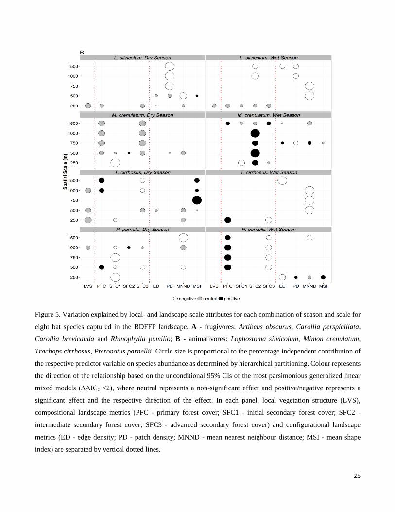
Figure 5. Variation explained by local- and landscape-scale attributes for each combination of season and scale for

eight bat species captured in the BDFFP landscape. A - frugivores: Artibeus obscurus, Carollia perspicillata,

Carollia brevicauda and Rhinophylla pumilio; B - animalivores: Lophostoma silvicolum, Mimon crenulatum,

Trachops cirrhosus, Pteronotus parnellii. Circle size is proportional to the percentage independent contribution of

the respective predictor variable on species abundance as determined by hierarchical partitioning. Colour represents

the direction of the relationship based on the unconditional 95% CIs of the most parsimonious generalized linear

mixed models (∆AICc <2), where neutral represents a non-significant effect and positive/negative represents a

significant effect and the respective direction of the effect. In each panel, local vegetation structure (LVS),

compositional landscape metrics (PFC - primary forest cover; SFC1 - initial secondary forest cover; SFC2 -

intermediate secondary forest cover; SFC3 - advanced secondary forest cover) and configurational landscape

metrics (ED - edge density; PD - patch density; MNND - mean nearest neighbour distance; MSI - mean shape

index) are separated by vertical dotted lines.

26

Discussion

We predicted that species would respond differently to landscape structure in each season and that these responses

would be scale- and species-specific. These assumptions were made based on the diverse biological and ecological

traits of bats and in view of the differences in food availability and distribution between wet and dry seasons, which

are affected by landscape characteristics. Responses were scale-dependent, species-specific, and seasonal, and were

affected by vegetation structure, and compositional and configurational metrics to varying degrees. Landscape-scale

were more important than local-scale in modulating the responses of bats, although the latter was associated with

two frugivores in the wet season. Nevertheless, our results did not support all of our predictions. Frugivores showed

a more distinctively seasonal pattern than animalivores, responding in the dry season more to compositional metrics

and more to local and configurational metrics in the wet season. Animalivorous species showed similar patterns in

both seasons, responding to the same group of metrics in the wet and dry season. Overall, secondary forest cover

was positively associated with the abundance of frugivores while negatively associated with the abundance of

animalivores, with responses being more marked for advanced secondary forest.

Influence of season and habitat type on bat abundance patterns

Capture rates were variable between seasons, with some species showing a clear seasonal pattern. Differences in

abundance occurred mostly in modified habitats (fragments, edge and matrix), probably due the different

chronology of flowering and fruiting events in the secondary forest matrix. In continuous terra firme forest, the

type of forest present at the BDFFP, fruiting pulses usually occur in the early wet season (Haugaasen & Peres 2005)

and consequently declines in frugivore abundances in primary forest are expected during the dry season (Ortêncio-

Filho et al. 2014). The reduction in food availability can lead to a shift of frugivores from primary to secondary

forest, where fruit availability can be less seasonal (Barlow et al. 2007b). Bentos et al. (2008) showed that at the

BDFFP some Cecropia spp. and Vismia spp., which are the dominant pioneer trees in the secondary forest matrix,

have their flowering and fruiting peaks during the dry season. Due to greater food availability, secondary forest

may be a more suitable habitat for some small generalist frugivores (de la Peña-Cuéllar et al. 2012; DeWalt et al.

2003; Faria 2006), which could lead to a change in their preferred foraging habitat during the dry season. It was

already shown in other areas that monkeys and birds shift their foraging habitat to regrowth forests when resources

in mature forests become scarce (Bowen et al. 2007). Despite this, none of the frugivorous bats showed an increase

in captures rates in continuous forest or in the fragments during the wet season, when food availability is higher.

An increase in fruit availability in other forest types (e.g. várzea forest) in comparison with terra firme forests

(Haugaasen & Peres 2005; Pereira et al. 2010) could explain the absence of this pattern. Bobrowiec et al. (2014)

showed that a drop in the abundance of Carollia spp in terra firme and a simultaneous increase in abundance of

the same species in várzea could indicate seasonal movements between these different forest types. Several studies

27

on birds also have documented a dominant effect of food availability on habitat selection (Burke & Nol 1998; Naoe

et al. 2011; Studds & Marra 2005). Therefore, such inter-habitat movements to other areas in the landscape could

mask the supposed increase in bat abundances in continuous forest during the wet season.

Seven of the eight frugivores analysed showed seasonal patterns whereas only three of six animalivores showed

differences between seasons. Compared with temperate species, many tropical insects tend to have long activity

periods with less marked seasonal pulses and with more constant abundances throughout the year, especially in

areas lacking a pronounced dry season (Hamer et al. 2005; Wolda 1988). However, some studies indicate that insect

availability is higher during the rainy season in the Neotropics (Beja et al. 2010; Ortêncio-Filho et al. 2014). This

fact can explain why some animalivores, although not significantly so, had high abundances in continuous forest

during the wet season (Tonatia saurophila) and other species had during the dry season (Mimon crenulatum and

Phyllostomus elongatus). Detailed studies on the dietary composition of Neotropical insectivorous bats are

necessary in order to know which insect families/species are present in each bat species’ diet and how they are

related to seasonal changes in abundance and availability of arthropods. Similarly, the lack of studies at BDFFP on

the insect and fruit abundance, as well on the diet of animalivorous and frugivorous bats, only allowed speculative

interpretations because differences in availability of food resources and bats diets can occur between regions.

Contrary to the other species, C. perspicillata and P. parnellii had higher abundances in fragments in the dry season.

Fragments in our study only comprised areas with a maximum of 100ha, i.e. much less than the known home range

of Carollia spp. Carollia species can have a home range above 1000ha (Bernard & Fenton 2003) and due to their

generalist diet and habitat affinities (Bobrowiec et al. 2014; Ortêncio-Filho et al. 2014) can easily use resources

from the secondary forest. P. parnellii is an aerial insectivore capable of foraging in narrow-space areas (Denzinger

& Schnitzler 2013). Morphological adaptations to flight in dense understory vegetation (de Oliveira et al. 2015;

Denzinger & Schnitzler 2013), may allow both C. perspicillata and P. parnellii to take advantage of secondary

forest areas for foraging and use primary forests as roosting sites.

Effects of seasonality on bat abundance responses to local and landscape-scale predictors

Seasonality affected the responses of bats to local and landscape metrics, with both groups of metrics playing an

important role in explaining how fragmentation affects bat abundances. As suggested by the results of model

consistency, which ranged from 0% to 71% and averaged 38.4%, responses varied substantially between seasons.

The relative importance of different predictor variables and the magnitude of their effect were dependent on the

season and species, in agreement with the findings of Klingbeil and Willig (2010) and Cisneros et al. (2015).

Similarly, Vergara and Marquet (2007) showed that the magnitude of the effects of landscape metrics in a bird

species were dependent on season. Even though fragment-matrix contrast at the BDFFP is low and distances

between fragments and continuous forest are relatively small, species were influenced by different environmental

filters that differ between seasons and benefit bat species depending on their biological and ecological traits

28

(Farneda et al. 2015). Both ensembles, frugivores and animalivores, responded differently to local, compositional

and configurational metrics and no clear patterns regarding responses at different spatial scales emerged. In a

parallel study conducted at the BDFFP, which used the same data, yet focused on responses at the assemblage-level,

Rocha et al. (submitted) showed that the direction of effect for species richness and total abundance was scale-

dependent, with e.g. species richness and total abundance being positively correlated with edge density at the

smallest spatial scales and negatively correlated at larger scales.

The low captures rates of most species during our study only allowed analysis to focus on the most abundant species

and consequently on more generalist species. Therefore, most of the rare and specialist bat species that depend

exclusively on primary forest were not included and should be considered in future studies involving seasonality.

Frugivore ensemble

In the dry season, frugivores responded more to compositional metrics whereas during the wet season local and

configurational metrics were more important. R. pumilio was an exception as it showed the opposite pattern.

Secondary forest can have greater fruit availability than primary forest during the dry season (Bentos et al. 2008;

Haugaasen & Peres 2005; Ortêncio-Filho et al. 2014), influencing the responses of frugivores that rely on these

resources. All frugivores were positively associated with advanced secondary forest cover (SFC3, age ≥ 16 years)

and negatively associated with primary forest cover (PFC), supporting the assumption that some generalist

frugivores prefer regrowth forests as foraging habitat in fragmented landscapes (Klingbeil & Willig 2009, 2010;

Montaño-Centellas et al. 2015).

For R. pumilio, overall, all configurational metrics were important during the dry season, with abundance being

positively associated with edge density at small scales. This suggests that although it can exploit resources in

secondary forest, the spatial organization of primary forest patches and distance between them play an important

role. These could be related to the small home range of this species, which ranges from 2.5ha to 16.9ha (Henry &

Kalko 2007) and to the fact that small scale edges can provide more foraging opportunities and improve connectivity

between roosting and foraging areas for this species (Kalda et al. 2015; Rocha et al. submitted). In the wet season,

R. pumilio responded more to compositional metrics. Female bats lactate at the onset and during the rainy season

(Estrada & Coates-Estrada 2001; Henry & Kalko 2007), increasing their food intake during this period (Henry &

Kalko 2007). Hence, during this period bats will be more dependent on food availability and distribution, responding

more to compositional metrics.

Carollia perspicillata was the only species that responded more to landscape composition (negatively to PFC and

positively to SFC3) than to the other group metrics in both the wet and dry season. In a study conducted in a

fragmented landscape characterized by continuous forest surrounded by matrix of agriculture, development and

logging areas, in unflooded (terra firme) Amazonian rainforest, Klingbeil and Willig (2010) found a consistent

29

negative response to primary forest (indicating a preference for secondary forest), regardless of season, for this

species. In our study, it represented more than 50% of all bat captures (Table S3), demonstrating its success in

exploiting the resources of secondary forest throughout the year. Fruit preferences can influence the foraging

behavior of species, and therefore can affect how they respond to landscape structure. C. perspicillata incorporates

great proportions of Vismia and Cecropia (the dominant tree genera in the BDFFP secondary forest matrix) in its

diet (Fleming 2004; Thies & Kalko 2004), explaining why its abundance was positively influenced by the amount

of secondary forest present in the landscape.

In the wet season, responses were more species-specific. A. obscurus and C. brevicauda responded more to local

vegetation structure than to landscape metrics in this season. Due to the high fruit availability during wet season

bats don’t need to travel long distances for foraging and consequently may be more dependent on the local-scale.

Local vegetation structure was negatively associated with the number of Vismia and Cecropia trees (Table S2),

which may explain why both species were negatively associated to local vegetation structure. This relation indicate

that these tree genera may also play an important role in the wet season. Cisneros et al. (2015) found that the

landscape metrics only influenced the metacommunity structure of the frugivore ensemble in the dry season and

suggested that environmental characteristics at the local scale could be more important in the wet season. Our

findings for both A. obscurus and C. brevicauda align with these assumption, and demonstrated that local vegetation

structure may play a more important role in the wet season for these two species.

In the wet season pregnant and lactating females bats can reduce their flight durations between foraging and roosting

sites in order to compensate for the metabolic cost of producing milk or the increased weight of carrying a fetus

(Charles-Dominique 1991; Klingbeil & Willig 2010). Moreover, males of some bats species (e.g. A. jamaicensis,

C. perspicillata) invest time and energy defending roosts and harems during the breeding season (Kunz & Hood

2000), which could result in smaller home ranges due to the higher energetic demands (Klingbeil & Willig 2010).

Therefore, the spatial scale at which bats respond may be smaller and more dependent on local vegetation structure

in the wet season. The spatial variability of food resources during the wet season in BDFFP landscape is more

heterogeneous and richer than in the dry season (see above) affecting the diet of frugivorous species. The diet of

some frugivorous species changes throughout the year as the food availability of different plant species varies across

the landscape (Da Silva et al. 2008). More studies are needed in order to understand how these complex relationships

between forest types affects the frugivore ensemble.

Animalivore ensemble

In contrast to frugivores, animalivores showed a more similar pattern between wet and dry season. Three of the

animalivorous species responded to the same group of metrics in both seasons, L. silvicolum to configuration and

P. parnellii and M. crenulatum to composition, suggesting that for animalivores, seasonality and consequently the

variability in resource availability may not play such an important role as it does for frugivores. This contrasts with

30

the findings of Klingbeil and Willig (2010), who found that abundance responses of animalivores to landscape

structure differed between seasons, responding to landscape configuration in the dry season and to landscape

composition in the wet season. However, their study was conducted in a more heterogeneous landscape, in which

primary forest was surrounded by agricultural, logging and development areas, whereas the primary forest

fragments at the BDFFP are surrounded by a more homogeneous matrix of secondary forest. Tews et al. (2004)

found a positive correlation between habitat heterogeneity/diversity and insect species diversity. Hence, the BDFFP

landscape could harbour a lower arthropod diversity and abundance than the matrix in Klingbeil and Willig (2010)

study, and consequently show a less seasonal variation in prey availability. In our study, only T. cirrhosus showed

seasonal variation in abundance, responding more to configurational metrics than composition in the wet season.

In the Neotropics, abundance of frugivores generally increases in fragmented or disturbed areas, whereas gleaning

animalivores tend to decline (Meyer et al. in press). Although late successional secondary forest can have structural

similarities to primary forest (Ferreira & Prance 1999), it can take decades or even centuries to resemble old-growth

forests (Guariguata and Ostertag, 2001). In our study landscape, most of the secondary forest in the matrix is less

than 30 years old (Carreiras et al. 2014) and consequently structurally less complex than adjacent continuous forest,

constituting less suitable habitat for most gleaning animalivores due to insufficient roosting and prey resources

(Meyer & Kalko 2008a). Therefore, most species will not be able to exploit the seasonal resource peaks that can

occur in secondary forest and will be more dependent on primary forests. With the exception of M. crenulatum, all

animalivorous species showed a negative association with secondary forest cover, edge density and mean nearest

neighbour distance in both seasons. Usually, higher density of edges and distances between patches lead to a

reduction in the quality of the landscape for species that have small home ranges and depend on primary forest. M.

crenulatum responded mostly to landscape composition and showed a positive relation with secondary forest cover,

especially with that of intermediate stages (SFC2, 6-15 years). Secondary forests of this age are structurally and

compositionally very different from primary forest (Guariguata & Ostertag 2001) and do not offer suitable habitat

conditions for most gleaners. However, our data indicate that M. crenulatum may be using secondary forest as

foraging area or as flyways between food patches, and should be considered a generalist species in terms of habitat

use. More information is nevertheless needed in order to understand if this species can really use sub-optimal

habitats or if this is an artefact of our data caused by the low capture rates of this species and the overall low

representation of intermediate-stage secondary forest in the landscape (less than 15% of all secondary forest).

As mentioned, T. cirrhosus responded more to configurational metrics in the wet season. Responses to

configurational metrics occur usually during the season when food availability is lower, because bats need to visit

habitat of lower quality (e.g. edges) and will be more dependent on the spatial arrangement and configuration of

forest patches (Klingbeil & Willig 2010). Trachops cirrhosus is a gleaning animalivore that feeds mainly on small

vertebrates, especially frogs, and insects (Kalko et al. 1999; Rodrigues et al. 2014). In the Central Amazon, the wet

season is the period of highest frog abundance and juvenile recruitment (Menin et al. 2008; Watling & Donnelly

31

2002). Despite this, T. cirrhosus showed a greater dependence on configurational metrics in the wet season,

suggesting that although frogs are consumed by the species at the BDFFP (Rocha et al. in press; Rocha et al. 2012),

this prey group may not be as important for T. cirrhosus in this area. Alternatively, fragmentation could be affecting

the phenology of its prey, leading to changes in the dietary habits of T. cirrhosus. Changes in dietary habitats in

fragmented landscapes due to reduced availability of high-value food resources have been documented for other

taxa such monkeys (Chaves et al. 2011). However, studies are needed in order to understand if fragmentation is

really affecting the dietary habits of T. cirrhosus.

Conclusions

Most bat species analysed in this study showed seasonal changes in abundance. Furthermore, seasonality affected

the responses of bats to local and landscape characteristics. Local-scale metrics were not as important as landscape-

scale metrics, however, for some species vegetation structure modulated the ecological responses to fragmentation

during the wet season. Differences in responses between seasons were likely a result of differential resource

availability and abundance that was intensified by fragmentation. The magnitude of seasonal changes in resource

availability can be affected by fragmentation, causing shifts in foraging strategy, and consequently the scale at

which species respond to landscape characteristics, that are probably not necessary in unfragmented landscapes

(Klingbeil & Willig 2010). Hence, it is necessary to understand how each species exploits the habitat and how its

dietary habits are jointly affected by fragmentation and seasonality, especially since synergistic effects between

fragmentation and seasonality may trigger cascading effects in plant-bat interactions, both directly via seed dispersal

and pollination or indirectly via the control of herbivorous arthropods. For example, Naoe et al. (2011) found that

seeds of tree species that fruit during the bird breeding season in fragmented areas were dispersed with less

efficiency that in continuous forest areas.

In our study area, where the contrast between fragments and matrix is low, most of the species were able to use the

secondary forest matrix to some degree. The conservation value of secondary forests in a future for which it is

predicted that up to 40% of the Amazon forest will be lost by 2050 (Soares-Filho et al. 2006) is tremendous, and

therefore knowledge about the ability of species to exploit the resources (food and roost) in secondary forest is

fundamental to improve the extinction risk assessment for bat species (Bird et al. 2012). Also, secondary forest can

be used as corridors to mitigate the impacts of deforestation, and allow the subsistence of frugivorous and

animalivorous bat populations (Bobrowiec & Gribel 2010). Our results indicate that advanced successional stages

of secondary forest constitute suitable habitats for frugivores but are not suitable for most gleaning animalivorous

bats. Therefore, management actions should promote secondary forest regrowth and consequently minimize

fragment - matrix contrast in order to maintain and improve habitat quality for bats. However, continuous primary

forests are areas of unique value and are essential to the preservation of tropical biodiversity (Barlow et al. 2007a;

Gibson et al. 2011), and so measures that prioritize the conservation of primary forest should prevail in conservation.

32

Finally, seasonality should be considered in management actions to guarantee that bats have the necessary resources

during non-breeding and breeding seasons.

References

Asner, G. P., D. E. Knapp, E. N. Broadbent, P. J. Oliveira, M. Keller, and J. N. Silva. 2005. Selective logging in

the Brazilian Amazon. Science 310:480-482.

Barlow, J., T. A. Gardner, I. S. Araujo, T. C. Ávila-Pires, A. B. Bonaldo, J. E. Costa, M. C. Esposito, L. V. Ferreira,

J. Hawes, M. I. M. Hernandez, M. S. Hoogmoed, R. N. Leite, N. F. Lo-Man-Hung, J. R. Malcolm, M. B.

Martins, L. A. M. Mestre, R. Miranda-Santos, A. L. Nunes-Gutjahr, W. L. Overal, L. Parry, S. L. Peters,

M. A. Ribeiro-Junior, M. N. F. da Silva, C. da Silva Motta, and C. A. Peres. 2007a. Quantifying the

biodiversity value of tropical primary, secondary, and plantation forests. Proceedings of the National

Academy of Sciences 104:18555-18560.

Barlow, J., L. A. M. Mestre, T. A. Gardner, and C. A. Peres. 2007b. The value of primary, secondary and plantation

forests for Amazonian birds. Biological Conservation 136:212-231.

Barlow, K., P. Briggs, K. Haysom, A. Hutson, N. Lechiara, P. Racey, A. Walsh, and S. Langton. 2015. Citizen

science reveals trends in bat populations: The National Bat Monitoring Programme in Great Britain.

Biological Conservation 182:14-26.

Bates, D. M. 2010. lme4: Mixed-effects modeling with R. URL http://lme4. r-forge. r-project. org/book.

Beja, P., C. Santos, J. Santana, M. Pereira, J. T. Marques, H. Queiroz, and J. Palmeirim. 2010. Seasonal patterns of

spatial variation in understory bird assemblages across a mosaic of flooded and unflooded Amazonian

forests. Biodiversity and Conservation 19:129-152.

Benchimol, M., and C. A. Peres. 2013. Anthropogenic modulators of species–area relationships in Neotropical

primates: a continental‐scale analysis of fragmented forest landscapes. Diversity and distributions 19:1339-

1352.

Benchimol, M., and C. A. Peres. 2015. Edge‐mediated compositional and functional decay of tree assemblages in

Amazonian forest islands after 26 years of isolation. Journal of Ecology.

Bentos, T. V., R. C. G. Mesquita, and G. B. Williamson. 2008. Reproductive phenology of Central Amazon pioneer

trees. . Trop. Conserv. Sci. 1: 186–203.

Bentos, T. V., H. E. M. Nascimento, and G. B. Williamson. 2013. Tree seedling recruitment in Amazon secondary

forest: Importance of topography and gap micro-site conditions. Forest Ecology and Management 287:140-

146.

Bernard, E., and M. B. Fenton. 2003. Bat Mobility and Roosts in a Fragmented Landscape in Central Amazonia,

Brazil. Biotropica 35:262-277.

Bird, J. P., G. M. Buchanan, A. C. Lees, R. P. Clay, P. F. Develey, I. Yépez, and S. H. Butchart. 2012. Integrating

spatially explicit habitat projections into extinction risk assessments: a reassessment of Amazonian avifauna

incorporating projected deforestation. Diversity and Distributions 18:273-281.

Bobrowiec, P. E. D., and R. Gribel. 2010. Effects of different secondary vegetation types on bat community

composition in Central Amazonia, Brazil. Animal Conservation 13:204-216.

Bobrowiec, P. E. D., L. d. S. Rosa, J. Gazarini, and T. Haugaasen. 2014. Phyllostomid bat assemblage structure in

Amazonian flooded and unflooded forests. Biotropica 46:312-321.

Bonthoux, S., J.-Y. Barnagaud, M. Goulard, and G. Balent. 2013. Contrasting spatial and temporal responses of

bird communities to landscape changes. Oecologia 172:563-574.

Bowen, M. E., C. A. McAlpine, A. P. N. House, and G. C. Smith. 2007. Regrowth forests on abandoned agricultural

land: A review of their habitat values for recovering forest fauna. Biological Conservation 140:273-296.

Bradshaw, C. J., N. S. Sodhi, and B. W. Brook. 2008. Tropical turmoil: a biodiversity tragedy in progress. Frontiers

in Ecology and the Environment 7:79-87.

Bregman, T. P., C. H. Sekercioglu, and J. A. Tobias. 2014. Global patterns and predictors of bird species responses

to forest fragmentation: implications for ecosystem function and conservation. Biological Conservation

169:372-383.

33

Brown Jr, K., and G. Prance. 1987. Soils and vegetation.

Burke, D. M., and E. Nol. 1998. Influence of food abundance, nest-site habitat, and forest fragmentation on breeding

ovenbirds. The Auk:96-104.

Burnham, K. P., and D. R. Anderson 2002. Model selection and multimodel inference: a practical information-

theoretic approach. Springer Science & Business Media.

Carreiras, J. M. B., J. Jones, R. M. Lucas, and C. Gabriel. 2014. Land Use and Land Cover Change Dynamics across

the Brazilian Amazon: Insights from Extensive Time-Series Analysis of Remote Sensing Data. PLoS ONE

9:e104144.

Castro, A., and C. Espinosa. 2015. Seasonal diversity of butterflies and its relationship with woody-plant resources

availability in an Ecuadorian tropical dry forest. Tropical Conservation Science 8.

Charles-Dominique, P. 1991. Feeding strategy and activity budget of the frugivorous bat Carollia perspicillata

(Chiroptera: Phyllostomidae) in French Guiana. Journal of Tropical Ecology 7:243-256.

Charles-Dominique, P., A. Brosset, and S. Jouard 2001. Les chauves-souris de Guyane. Muséum national d'histoire

naturelle, Laboratoire d'écologie générale.

Chaves, Ó. M., K. E. Stoner, and V. Arroyo-Rodríguez. 2011. Seasonal Differences in Activity Patterns of

Geoffroyi´ s Spider Monkeys (Ateles geoffroyi) Living in Continuous and Fragmented Forests in Southern

Mexico. International Journal of Primatology 32:960-973.

Chazdon, R. L., C. A. Peres, D. Dent, D. Sheil, A. E. Lugo, D. Lamb, N. E. Stork, and S. E. Miller. 2009. The

potential for species conservation in tropical secondary forests. Conservation Biology 23:1406-1417.

Chevan, A., and M. Sutherland. 1991. Hierarchical Partitioning. The American Statistician 45:90-96.

Cisneros, L. M., M. E. Fagan, and M. R. Willig. 2014. Effects of human‐modified landscapes on taxonomic,

functional and phylogenetic dimensions of bat biodiversity. Diversity and Distributions 21:523-533.

Cisneros, L. M., M. E. Fagan, and M. R. Willig. 2015. Season-specific and guild-specific effects of anthropogenic

landscape modification on metacommunity structure of tropical bats. Journal of Animal Ecology 84:373-

385.

Da Silva, A. G., O. Gaona, and R. A. Medellín. 2008. Diet and trophic structure in a community of fruit-eating bats

in Lacandon Forest, Mexico. Journal of Mammalogy 89:43-49.

de la Peña-Cuéllar, E., K. Stoner, L. Avila-Cabadilla, M. Martínez-Ramos, and A. Estrada. 2012. Phyllostomid bat

assemblages in different successional stages of tropical rain forest in Chiapas, Mexico. Biodiversity and

Conservation 21:1381-1397.

de Oliveira, L. Q., R. Marciente, W. E. Magnusson, and P. E. D. Bobrowiec. 2015. Activity of the insectivorous bat

Pteronotus parnellii relative to insect resources and vegetation structure. Journal of Mammalogy:gyv108.

Denzinger, A., and H.-U. Schnitzler. 2013. Bat guilds, a concept to classify the highly diverse foraging and

echolocation behaviors of microchiropteran bats. Frontiers in physiology 4.

DeWalt, S. J., S. K. Maliakal, and J. S. Denslow. 2003. Changes in vegetation structure and composition along a

tropical forest chronosequence: implications for wildlife. Forest Ecology and Management 182:139-151.

Dirzo, R., H. S. Young, M. Galetti, G. Ceballos, N. J. B. Isaac, and B. Collen. 2014. Defaunation in the

Anthropocene. Science 345:401-406.

Dormann, C. F., J. Elith, S. Bacher, C. Buchmann, G. Carl, G. Carré, J. R. G. Marquéz, B. Gruber, B. Lafourcade,

and P. J. Leitão. 2013. Collinearity: a review of methods to deal with it and a simulation study evaluating

their performance. Ecography 36:27-46.

Durant, K. A., R. W. Hall, L. M. Cisneros, R. M. Hyland, and M. R. Willig. 2013. Reproductive phenologies of

phyllostomid bats in Costa Rica. Journal of Mammalogy 94:1438-1448.

Erickson, J. L., and S. D. West. 2003. Associations of bats with local structure and landscape features of forested

stands in western Oregon and Washington. Biological Conservation 109:95-102.

Estrada, A., and R. Coates-Estrada. 2001. Species composition and reproductive phenology of bats in a tropical

landscape at Los Tuxtlas, Mexico. Journal of Tropical Ecology 17:627-646.

Ewers, R. M., and C. Banks-Leite. 2013. Fragmentation impairs the microclimate buffering effect of tropical forests.

PLOS one 8:e58093.

Ewers, R. M., and R. K. Didham. 2006. Confounding factors in the detection of species responses to habitat

fragmentation. Biological Reviews 81:117-142.

34

Faria, D. 2006. Phyllostomid bats of a fragmented landscape in the north-eastern Atlantic forest, Brazil. Journal of

Tropical Ecology 22:531-542.

Farneda, F. Z., R. Rocha, A. López-Baucells, M. Groenenberg, I. Silva, J. M. Palmeirim, P. E. D. Bobrowiec, and

C. F. J. Meyer. 2015. Trait-related responses to habitat fragmentation in Amazonian bats. Journal of Applied

Ecology 52:1381-1391.

Fearnside, P. M. 2001. Soybean cultivation as a threat to the environment in Brazil. Environmental Conservation

28:23-38.

Fenton, M. B., and N. B. Simmons 2015. Bats: a world of science and mystery. University of Chicago Press.

Ferraz, G., G. J. Russell, P. C. Stouffer, R. O. Bierregaard, S. L. Pimm, and T. E. Lovejoy. 2003. Rates of species

loss from Amazonian forest fragments. Proceedings of the National Academy of Sciences 100:14069-

14073.

Ferreira, L. V., and G. T. Prance. 1999. Ecosystem recovery in terra firme forests after cutting and burning: a

comparison on species richness, floristic composition and forest structure in the Jaú National Park,

Amazonia. Botanical Journal of the Linnean Society 130:97-110.

Figueira, L., J. L. Tella, U. M. Camargo, and G. Ferraz. 2015. Autonomous sound monitoring shows higher use of

Amazon old growth than secondary forest by parrots. Biological Conservation 184:27-35.

Fleming, T. H. 2004. Dispersal ecology of neotropical Piper shrubs and treelets. Pages 58-77. Piper: a model genus

for studies of phytochemistry, ecology, and evolution. Springer.

García-García, J. L., A. Santos-Moreno, and C. Kraker-Castañeda. 2014. Ecological traits of phyllostomid bats

associated with sensitivity to tropical forest fragmentation in Los Chimalapas, Mexico. Tropical

Conservation Science 7 457-474.

García‐Morales, R., E. I. Badano, and C. E. Moreno. 2013. Response of Neotropical bat assemblages to human land

use. Conservation Biology 27:1096-1106.

Gardner, A. L. 2008. Mammals of South America, volume 1: marsupials, xenarthrans, shrews, and bats. University

of Chicago Press.

Gascon, C., T. E. Lovejoy, R. O. Bierregaard Jr, J. R. Malcolm, P. C. Stouffer, H. L. Vasconcelos, W. F. Laurance,

B. Zimmerman, M. Tocher, and S. Borges. 1999. Matrix habitat and species richness in tropical forest

remnants. Biological Conservation 91:223-229.

Gibson, L., T. M. Lee, L. P. Koh, B. W. Brook, T. A. Gardner, J. Barlow, C. A. Peres, C. J. Bradshaw, W. F.

Laurance, and T. E. Lovejoy. 2011. Primary forests are irreplaceable for sustaining tropical biodiversity.

Nature 478:378-381.

Goosem, M. 1997. Internal fragmentation: the effects of roads, highways, and powerline clearings on movements

and mortality of rainforest vertebrates. Tropical forest remnants: ecology, management, and conservation

of fragmented communities. University of Chicago Press, Chicago:241-255.

Guariguata, M. R., and R. Ostertag. 2001. Neotropical secondary forest succession: changes in structural and

functional characteristics. Forest ecology and management 148:185-206.

Gutzwiller, K. J., and W. C. Barrow Jr. 2001. Bird-landscape relations in the Chihuahuan Desert: coping with

uncertainties about predictive models. Ecological Applications 11:1517-1532.

Hamer, K. C., J. K. Hill, N. Mustaffa, S. Benedick, T. N. Sherratt, V. K. Chey, and M. Maryati. 2005. Temporal

variation in abundance and diversity of butterflies in Bornean rain forests: opposite impacts of logging

recorded in different seasons. Journal of Tropical Ecology 21:417-425.

Haugaasen, T., and C. A. Peres. 2005. Tree Phenology in Adjacent Amazonian Flooded and Unflooded Forests1.

Biotropica 37:620-630.

Henry, M., and E. K. Kalko. 2007. Foraging strategy and breeding constraints of Rhinophylla pumilio

(Phyllostomidae) in the Amazon lowlands. Journal of Mammalogy 88:81-93.

Hothorn, T., F. Bretz, and M. T. Hothorn. 2007. The multcomp package.

INPA. 2014. National Institute of Amazonian Research: Precipitation data (2011-2013).

Jones, G., D. S. Jacobs, T. H. Kunz, M. R. Willig, and P. A. Racey. 2009. Carpe noctem: the importance of bats as

bioindicators. Endangered Species Research 8:93-115.

Kalda, R., O. Kalda, K. Lõhmus, and J. Liira. 2015. Multi-scale ecology of woodland bat the role of species pool,

landscape complexity and stand structure. Biodiversity and Conservation 24:337-353.

35

Kalko, E. 1998. Organisation and diversity of tropical bat communities through space and time. Zoology 101:281-

297.

Kalko, E. K. V., D. Friemel, C. O. Handley, and H.-U. Schnitzler. 1999. Roosting and Foraging Behavior of Two

Neotropical Gleaning Bats, Tonatia silvicola and Trachops cirrhosus (Phyllostomidae). Biotropica 31:344-

353.

Kattan, G. H., H. Alvarez‐López, and M. Giraldo. 1994. Forest fragmentation and bird extinctions: San Antonio

eighty years later. Conservation Biology 8:138-146.

Klingbeil, B. T., and M. R. Willig. 2009. Guild-specific responses of bats to landscape composition and

configuration in fragmented Amazonian rainforest. Journal of Applied Ecology 46:203-213.

Klingbeil, B. T., and M. R. Willig. 2010. Seasonal differences in population-, ensemble- and community-level

responses of bats to landscape structure in Amazonia. Oikos 119:1654-1664.

Kunz, T. H., E. Braun de Torrez, D. Bauer, T. Lobova, and T. H. Fleming. 2011. Ecosystem services provided by

bats. Annals of the New York Academy of Sciences 1223:1-38.

Kunz, T. H., and W. R. Hood. 2000. Parental care and postnatal growth in the Chiroptera. Reproductive biology of

bats:415-468.

Kupfer, J. A., G. P. Malanson, and S. B. Franklin. 2006. Not seeing the ocean for the islands: the mediating influence

of matrix‐based processes on forest fragmentation effects. Global ecology and biogeography 15:8-20.

Laurance, S. G. W., P. C. Stouffer, and W. F. Laurance. 2004. Effects of Road Clearings on Movement Patterns of

Understory Rainforest Birds in Central Amazonia. Efectos de los Claros de Caminos sobre Patrones de

Movimiento de Aves de Sotobosque en la Amazonía Central. Conservation Biology 18:1099-1109.

Laurance, W. F., J. L. C. Camargo, R. C. C. Luizão, S. G. Laurance, S. L. Pimm, E. M. Bruna, P. C. Stouffer, G.

Bruce Williamson, J. Benítez-Malvido, H. L. Vasconcelos, K. S. Van Houtan, C. E. Zartman, S. A. Boyle,

R. K. Didham, A. Andrade, and T. E. Lovejoy. 2011. The fate of Amazonian forest fragments: A 32-year

investigation. Biological Conservation 144:56-67.

Laurance, W. F., T. E. Lovejoy, H. L. Vasconcelos, E. M. Bruna, R. K. Didham, P. C. Stouffer, C. Gascon, R. O.

Bierregaard, S. G. Laurance, and E. Sampaio. 2002. Ecosystem Decay of Amazonian Forest Fragments: a

22-Year Investigation. Descomposición del Ecosistema en Fragmentos de Bosque Amazónico, Una

Investigación de 22 Años. Conservation Biology 16:605-618.

Laurance, W. F., J. Sayer, and K. G. Cassman. 2014. Agricultural expansion and its impacts on tropical nature.

Trends in ecology & evolution 29:107-116.

Lim, B. K., and M. D. Engstrom. 2001. Species diversity of bats (Mammalia: Chiroptera) in Iwokrama Forest,

Guyana, and the Guianan subregion: implications for conservation. Biodiversity & Conservation 10:613-

657.

Lobova, T. A., C. K. Geiselman, and S. A. Mori 2009. Seed dispersal by bats in the Neotropics. New York Botanical

Garden.

Lovejoy, T. E., R. Bierregaard Jr, A. Rylands, J. Malcolm, C. Quintela, L. Harper, K. Brown Jr, A. Powell, G.

Powell, and H. Schubart. 1986. Edge and other effects of isolation on Amazon forest fragments.

Lovejoy, T. E., and R. Bierregaard. 1990. Central Amazonian forests and the minimum critical size of ecosystems

project. Four neotropical rainforests:60-71.

Maas, B., D. S. Karp, S. Bumrungsri, K. Darras, D. Gonthier, J. C. C. Huang, C. A. Lindell, J. J. Maine, L. Mestre,

and N. L. Michel. 2015. Bird and bat predation services in tropical forests and agroforestry landscapes.

Biological Reviews.

Mac Nally, R. 2000. Regression and model-building in conservation biology, biogeography and ecology: the

distinction between–and reconciliation of–‘predictive’and ‘explanatory’models. Biodiversity &

Conservation 9:655-671.

MacArthur, R. H. 1972. Geographical ecology: patterns in the distribution of species. Princeton University Press.

Maldonado-Coelho, M., and M. A. Marini. 2004. Mixed-species bird flocks from Brazilian Atlantic forest: the

effects of forest fragmentation and seasonality on their size, richness and stability. Biological Conservation

116:19-26.

36

Marques, J. T., M. J. Ramos Pereira, T. A. Marques, C. D. Santos, J. Santana, P. Beja, and J. M. Palmeirim. 2013.

Optimizing Sampling Design to Deal with Mist-Net Avoidance in Amazonian Birds and Bats. PLoS ONE

8:e74505.

Mazerolle, M. J., and M. M. J. Mazerolle. 2015. Package ‘AICcmodavg’.

McGarigal, K. 2014. FRAGSTATS HELP.

McGarigal, K., and W. C. McComb. 1995. Relationships between landscape structure and breeding birds in the

Oregon Coast Range. Ecological monographs 65:235-260.

Mello, M. A. R. 2009. Temporal variation in the organization of a Neotropical assemblage of leaf-nosed bats

(Chiroptera: Phyllostomidae). Acta Oecologica 35:280-286.

Melo, F. P., V. Arroyo-Rodríguez, L. Fahrig, M. Martínez-Ramos, and M. Tabarelli. 2013. On the hope for

biodiversity-friendly tropical landscapes. Trends in ecology & evolution 28:462-468.

Mendenhall, C. D., D. S. Karp, C. F. J. Meyer, E. A. Hadly, and G. C. Daily. 2014. Predicting biodiversity change

and averting collapse in agricultural landscapes. Nature 509:213-217.

Menin, M., F. Waldez, and A. P. Lima. 2008. Temporal variation in the abundance and number of species of frogs

in 10,000 ha of a forest in Central Amazonia, Brazil. South American Journal of Herpetology 3:68-81.

Mesquita, R. C., K. Ickes, G. Ganade, and G. B. Williamson. 2001. Alternative successional pathways in the

Amazon Basin. Journal of Ecology 89:528-537.

Meyer, C. F. J., and E. K. V. Kalko. 2008a. Assemblage-level responses of phyllostomid bats to tropical forest

fragmentation: land-bridge islands as a model system. Journal of Biogeography 35:1711-1726.

Meyer, C. F. J., and E. K. V. Kalko. 2008b. Bat assemblages on Neotropical land-bridge islands: nested subsets and

null model analyses of species co-occurrence patterns. Diversity and Distributions 14:644-654.

Meyer, C. F. J., M. Struebig, and M. R. Willig. in press. Responses of tropical bats to habitat fragmentation, logging,

and deforestation in C. C. Voigt, and T. Kingston, editors. Bats in the Anthropocene: Conservation of bats

in a changing world. Springer.

Montaño-Centellas, F., M. I. Moya, L. F. Aguirre, R. Galeón, O. Palabral, R. Hurtado, I. Galarza, and J. Tordoya.

2015. Community and species-level responses of phyllostomid bats to a disturbance gradient in the tropical

Andes. Acta Oecologica 62:10-17.

Nally, R., and C. Walsh. 2004. Hierarchical Partitioning Public-domain Software. Biodiversity & Conservation

13:659-660.

Naoe, S., S. Sakai, A. Sawa, and T. Masaki. 2011. Seasonal difference in the effects of fragmentation on seed

dispersal by birds in Japanese temperate forests. Ecological research 26:301-309.

Ortêncio-Filho, H., T. E. Lacher, and L. C. Rodrigues. 2014. Seasonal patterns in community composition of bats

in forest fragments of the Alto Rio Paraná, southern Brazil. Studies on Neotropical Fauna and Environment

49:169-179.

Patterson, B. D., M. R. Willig, and R. D. Stevens. 2003. Trophic strategies, niche partitioning, and patterns of

ecological organization. Bat ecology 9:536-557.

Pereira, M. J., J. T. Marques, and J. M. Palmeirim. 2010. Ecological Responses of Frugivorous Bats to Seasonal

Fluctuation in Fruit Availability in Amazonian Forests. Biotropica 42:680-687.

Peres, C. A. 2001. Synergistic effects of subsistence hunting and habitat fragmentation on Amazonian forest

vertebrates. Conservation Biology 15:1490-1505.

Quesada, M., K. E. Stoner, J. A. Lobo, Y. Herrerias‐Diego, C. Palacios‐Guevara, M. A. Munguía‐Rosas, O. Salazar,

A. Karla, and V. Rosas‐Guerrero. 2004. Effects of Forest Fragmentation on Pollinator Activity and

Consequences for Plant Reproductive Success and Mating Patterns in Bat‐pollinated Bombacaceous

Trees1. Biotropica 36:131-138.

R Development Core Team. 2013. R: a Language and Environment for Statistical Computing. R Foundation for

Statistical Computing, Vienna, Austria.

Rebelo, H., P. Tarroso, and G. Jones. 2010. Predicted impact of climate change on European bats in relation to their

biogeographic patterns. Global Change Biology 16:561-576.

Rocha, R., M. Gordo, and A. López-Baucells. in press. Completing the menu: addition of Sinax ruber and

Dendropsophus minutus (Anura: Hylidae) to the diet of Trachops cirrhosus (Chiroptera: Phyllostomidae)

in Central Amazon. North-Western Journal of Zoology.

37

Rocha, R., A. López-Baucells, F. Z. Farneda, M. Groenenberg, P. E. D. Bobrowiec, M. Cabeza, J. M. Palmeirim,

and C. F. J. Meyer. submitted. Consequences of a large-scale fragmentation experiment for Neotropical

bats: disentangling the relative importance of local and landscape-scale effects.

Rocha, R., I. Silva, A. Marajó dos Reis, and G. M. Rosa. 2012. Another frog on the menu: predation of Trachops

cirrhosus (Chiroptera: Phyllostomidae) upon Osteocephalus oophagus (Anura: Hylidae). Chiroptera

Neotropical 18:1136-1138.

Rodrigues, F. H., M. L. Reis, and V. S. Braz. 2014. Food habits of the frog-eating bat, Trachops cirrhosus, in

Atlantic Forest of Northeastern Brazil. Chiroptera Neotropical 10:180-182.

Schipper, J., J. S. Chanson, F. Chiozza, N. A. Cox, M. Hoffmann, V. Katariya, J. Lamoreux, A. S. Rodrigues, S. N.

Stuart, and H. J. Temple. 2008. The status of the world's land and marine mammals: diversity, threat, and

knowledge. Science 322:225-230.

Smith, A. C., N. Koper, C. M. Francis, and L. Fahrig. 2009. Confronting collinearity: comparing methods for

disentangling the effects of habitat loss and fragmentation. Landscape Ecology 24:1271-1285.

Soares-Filho, B. S., D. C. Nepstad, L. M. Curran, G. C. Cerqueira, R. A. Garcia, C. A. Ramos, E. Voll, A.

McDonald, P. Lefebvre, and P. Schlesinger. 2006. Modelling conservation in the Amazon basin. Nature

440:520-523.

Struebig, M. J., T. Kingston, A. Zubaid, A. Mohd-Adnan, and S. J. Rossiter. 2008. Conservation value of forest

fragments to Palaeotropical bats. Biological Conservation 141:2112-2126.

Studds, C. E., and P. P. Marra. 2005. Nonbreeding habitat occupancy and population processes: an upgrade

experiment with a migratory bird. Ecology 86:2380-2385.

Tews, J., U. Brose, V. Grimm, K. Tielbörger, M. Wichmann, M. Schwager, and F. Jeltsch. 2004. Animal species

diversity driven by habitat heterogeneity/diversity: the importance of keystone structures. Journal of

biogeography 31:79-92.

Thies, W., and E. K. Kalko. 2004. Phenology of neotropical pepper plants (Piperaceae) and their association with

their main dispersers, two short‐tailed fruit bats, Carollia perspicillata and C. castanea (Phyllostomidae).

Oikos 104:362-376.

VanDerWal, J., L. Falconi, S. Januchowski, L. Shoo, C. Storlie, and M. J. VanDerWal. 2011. Package ‘SDMTools’.

Vergara, P. M., and P. A. Marquet. 2007. On the seasonal effect of landscape structure on a bird species: the thorn-

tailed rayadito in a relict forest in northern Chile. Landscape ecology 22:1059-1071.

Watling, J. I., and M. A. Donnelly. 2002. Seasonal patterns of reproduction and abundance of leaf litter frogs in a

Central American rainforest. Journal of Zoology 258:269-276.

Watson, J. E., R. J. Whittaker, and T. P. Dawson. 2004. Habitat structure and proximity to forest edge affect the

abundance and distribution of forest-dependent birds in tropical coastal forests of southeastern Madagascar.

Biological Conservation 120:311-327.

Williamson, G., J. Longworth, T. Bentos, and R. Mesquita. 2012. Rates of change in tree communities along

alternative successional pathways in the Central Amazon. Plant Ecology and Diversity.

Wolda, H. 1988. Insect Seasonality: Why? Annual Review of Ecology and Systematics 19:1-18.

Wright, S. J. 2005. Tropical forests in a changing environment. Trends in Ecology & Evolution 20:553-560.

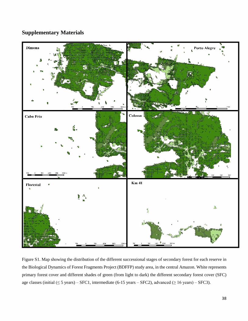
38

Supplementary Materials

Figure S1. Map showing the distribution of the different successional stages of secondary forest for each reserve in

the Biological Dynamics of Forest Fragments Project (BDFFP) study area, in the central Amazon. White represents

primary forest cover and different shades of green (from light to dark) the different secondary forest cover (SFC)

age classes (initial (≤ 5 years) – SFC1, intermediate (6-15 years – SFC2), advanced (≥ 16 years) – SFC3).

39

Table S1. Summary of local vegetation structure variables. CC = percent canopy cover, CH = canopy height (m), DBH = average (cm) of the DBH measures

of trees ≥ 10 cm, L = number of lianas, P = number of palms, S = number of woody stems (DBH < 10 cm), T = number of trees (DBH ≥ 10 cm), VC =

number of Vismia and Cecropia trees, VFD = vertical foliage density. Results are presented as mean ± 1SD. Taken from Rocha et al. (submitted).

Habitat category CC CH DBH L P S T VC VFD

Continuous forest interior 85.4 ± 5.2 12.4 ± 3.2 24.8 ± 1.3 1.2 ± 0.4 14.4 ± 5.1 101.1 ± 27.8 10.9 ± 2.7 0.2 ± 0.4 519.4 ± 112.8

Continuous forest edge 78.6 ± 5.3 7.8 ± 1.8 17.7 ± 1.5 1.7 ± 1.2 5.7 ± 3.2 70.3 ± 10.7 11.3 ± 2.1 1.7 ± 0.6 455.3 ± 134.3

Continuous forest matrix 79.1 ± 0.3 8.6 ± 2.8 16.3 ± 1.5 1.7 ± 0.6 4.7 ± 2.1 83.7 ± 43 9.3 ± 1.2 2.3 ± 1.5 460.3 ± 164.1

100 ha fragment interior 83.6 ± 0.9 11.3 ± 1.6 23 ± 1.4 1 10.5 ± 6.4 92 ± 29.7 8 0 722.5 ± 98.3

100 ha fragment edge 74.2 ± 5.5 8.7 ± 0.6 17.5 ± 0.7 2.5 ± 0.7 4.5 ± 2.1 109.5 ± 13.4 11 ± 1.4 3 575 ± 89.1

100 ha fragment matrix 71.6 ± 2 7.1 ± 0.5 17 ± 1.4 2.5 ± 2.1 2 ± 2.8 105 ± 28.3 7.5 ± 0.7 2 463 ± 1.4

10 ha fragment interior 87.4 ± 1 9.7 ± 1.2 23 ± 3 2.3 ± 1.2 7 ± 1 96 ± 15.6 7.7 ± 0.6 0.7 ± 0.6 639 ± 53.7

10 ha fragment edge 79.6 ± 2.5 6.7 ± 0.6 20.7 ± 6.4 3 ± 1 4.7 ± 2.1 123.3 ± 54.2 8.7 ± 1.5 9.3 ± 10.2 438 ± 67.9

10 ha fragment matrix 76.5 ± 1.3 6.6 ± 1.5 14.3 ± 1.5 1.7 ± 2.1 2.7 ± 2.1 117.7 ± 32.1 8.3 ± 4.9 12.3 ± 9.3 362.7 ± 29.5

1 ha fragment interior 84.6 ± 2 7.6 ± 0.7 23.3 ± 3.8 2 ± 1 11 ± 5 88 ± 42.5 7.7 ± 0.6 0 547.7 ± 89.4

1 ha fragment edge 79.1 ± 10.2 7.1 ± 0.8 18 ± 3.6 2.3 ± 1.5 5 ± 4 130 ± 34.7 10 ± 2.6 2.3 ± 2.1 519 ± 24

1 ha fragment matrix 75.1 ± 6.7 7.3 ± 1.7 18.3 ± 2.3 3.3 ± 0.6 5 ± 3.6 95.3 ± 25.8 7.3 ± 2.3 4.3 ± 3.2 468.3 ± 137

40

Figure S2. Principal component analysis examining the covariation between local vegetation structure variables. CC = canopy cover, CH = canopy height

(m), DBH = average of the DBH measures of trees ≥10 cm, L = number of lianas, P = number of palms, S = number of woody stems (DBH <10 cm), T =

number of trees (DBH >10), VC = number of Vismia and Cecropia trees, VFD = vertical foliage density.

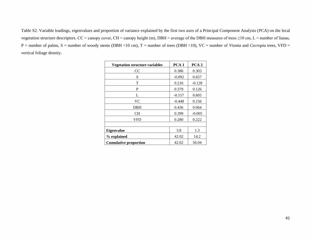
41

Table S2. Variable loadings, eigenvalues and proportion of variance explained by the first two axes of a Principal Component Analysis (PCA) on the local

vegetation structure descriptors. CC = canopy cover, CH = canopy height (m), DBH = average of the DBH measures of trees ≥10 cm, L = number of lianas,

P = number of palms, S = number of woody stems (DBH <10 cm), T = number of trees (DBH >10), VC = number of Vismia and Cecropia trees, VFD =

vertical foliage density.

Vegetation structure variables PCA 1 PCA 2

CC 0.386 0.303

S -0.092 0.657

T 0.216 -0.128

P 0.379 0.126

L -0.157 0.605

VC -0.448 0.156

DBH 0.436 0.064

CH 0.399 -0.005

VFD 0.280 0.222

Eigenvalue 3.8 1.3

% explained 42.02 14.2

Cumulative proportion 42.02 56.04

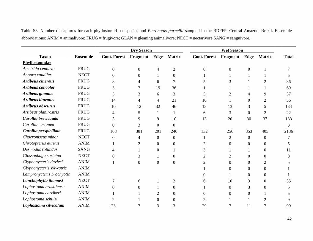
42

Table S3. Number of captures for each phyllostomid bat species and Pteronotus parnellii sampled in the BDFFP, Central Amazon, Brazil. Ensemble

abbreviations: ANIM = animalivore; FRUG = frugivore; GLAN = gleaning animalivore; NECT = nectarivore SANG = sanguivore.

Dry Season Wet Season

Taxon Ensemble Cont. Forest Fragment Edge Matrix Cont. Forest Fragment Edge Matrix Total

Phyllostomidae

Ametrida centurio FRUG 0 0 4 2 0 0 0 1 7

Anoura caudifer NECT 0 0 1 0 1 1 1 1 5

Artibeus cinereus FRUG 8 4 6 7 5 3 1 2 36

Artibeus concolor FRUG 3 7 19 36 1 1 1 1 69

Artibeus gnomus FRUG 5 3 6 3 5 2 4 9 37

Artibeus lituratus FRUG 14 4 4 21 10 1 0 2 56

Artibeus obscurus FRUG 10 12 32 46 13 13 3 5 134

Artibeus planirostris FRUG 4 5 1 1 6 3 0 2 22

Carollia brevicauda FRUG 5 9 9 10 13 20 30 37 133

Carollia castanea FRUG 0 3 0 0 3

Carollia perspicillata FRUG 168 381 201 240 132 256 353 405 2136

Choeroniscus minor NECT 0 4 0 0 1 2 0 0 7

Chrotopterus auritus ANIM 1 2 0 0 2 0 0 0 5

Desmodus rotundus SANG 4 1 0 1 3 1 1 0 11

Glossophaga soricina NECT 0 3 1 0 2 2 0 0 8

Glyphonycteris daviesi ANIM 1 0 0 0 2 0 0 2 5

Glyphonycteris sylvestris ANIM 1 0 0 0 1

Lampronycteris brachyotis ANIM 0 1 0 0 1

Lonchophylla thomasi NECT 7 6 1 2 6 10 3 0 35

Lophostoma brasiliense ANIM 0 0 1 0 1 0 3 0 5

Lophostoma carrikeri ANIM 1 1 2 0 0 0 0 1 5

Lophostoma schulzi ANIM 2 1 0 0 2 1 1 2 9

Lophostoma silvicolum ANIM 23 7 3 3 29 7 11 7 90

43

Mesophylla macconnelli FRUG 12 2 1 1 4 3 1 0 24

Micronycteris hirsuta ANIM 0 1 0 0 0 0 0 1 2

Micronycteris megalotis ANIM 1 1 0 1 0 0 1 0 4

Micronycteris microtis ANIM 2 1 0 1 3 2 2 4 15

Micronycteris schmidtorum ANIM 0 1 0 0 1

Mimon crenulatum ANIM 20 6 7 7 6 10 20 16 92

Phylloderma stenops ANIM 1 3 0 1 6 0 3 2 16

Phyllostomus discolor NECT 2 3 1 0 1 0 2 1 10

Phyllostomus elongatus ANIM 16 4 1 0 5 3 3 1 33

Phyllostomus hastatus ANIM 1 1 1 0 3

Platyrrhinus helleri FRUG 0 0 2 0 0 0 0 1 3

Rhinophylla pumilio FRUG 63 108 34 37 54 72 90 86 544

Sturnira tildae FRUG 1 1 1 7 0 0 4 12 26

Tonatia saurophila ANIM 9 10 2 1 23 15 4 3 67

Trachops cirrhosus ANIM 27 7 4 2 44 23 4 14 125

Trinycteris nicefori ANIM 2 0 0 0 2 2 2 2 10

Uroderma bilobatum FRUG 0 1 2 0 0 0 0 2 5

Vampyressa pusilla FRUG 0 0 1 0 1

Vampyriscus bidens FRUG 3 3 0 1 7 2 1 2 19

Vampyriscus brocki FRUG 0 1 0 0 0 1 1 0 3

Mormoopidae

Pteronotus parnellii ANIM 47 40 11 16 71 13 36 38 272

Total Captures 462 646 357 447 462 471 588 662 4095

44

Table S4. Results of the Likelihood ratio test for the abundance of each species between seasons (dry and wet) and habitat types (interior, edge and

matrix). Significant (adjusted P < 0.05) results are highlighted in bold.

Interaction (Season x Habitat Type) Season Habitat Type

Species Pr (>Chisq) Chisq Df Pr (>Chisq) Chisq Df Pr (>Chisq) Chisq Df

Artibeus cinereus 0.0051 20.239 7 0.0005 11.98 1 0.6498 1.64 3

Artibeus concolor < 2.2e-16 134.76 7 < 2.2e-16 111.27 1 0.0022 14.55 3

Artibeus gnomus 0.3649 7.6459 7 0.4975 0.46 1 0.271 3.91 3

Artibeus lituratus 4.626e-11 62.568 7 4.735e-08 29.82 1 0.0036 13.55 3

Artibeus obscurus < 2.2e-16 134.71 7 < 2.2e-16 76.88 1 0.9863 0.14 3

Carollia brevicauda 0.0009 24.628 7 0.0006 11.75 1 0.004 13.32 3

Carollia perspicillata 1.96e-10 59.431 7 3.719e-11 43.76 1 0.007 12.10 3

Lophostoma silvicolum 0.2218 9.4524 7 0.5401 0.38 1 0.0387 8.38 3

Lonchophylla thomasi 0.061 13.492 7 0.7867 0.07 1 0.0502 7.81 3

Mimon crenulatum 0.2097 9.644 7 0.6297 0.23 1 0.3915 3.00 3

Phyllostomus elongatus 0.0437 14.453 7 0.0266 4.92 1 0.0573 7.51 3

Pteronotus parnellii 0.0007 25.28 7 0.6546 0.20 1 0.2929 3.72 3

Rhinophylla pumilio 0.0068 19.498 7 0.2262 1.46 1 0.016 10.33 3

Trachops cirrhosus 0.0006 25.782 7 0.0068 7.32 1 0.0168 10.22 3

Tonatia saurophila 0.0263 15.871 7 0.0319 4.60 1 0.0362 8.53 3

45

Table S5. Results of multiple pairwise comparisons of GLMMs testing for differences in abundance of eleven species across the two seasons (dry and wet)

and across the four habitat types (continuous forest, fragment, edge and matrix). Significant (adjusted P < 0.05) results are highlighted in bold.

Wet vs Dry Species Wet vs Dry Species

Artibeus cinereus Phyllostomus elongatus

Estimate Std. Error z value Pr(>|z|) Estimate Std. Error z value Pr(>|z|)

Cont. Forest -0.7019 0.6124 -1.146 0.942 Cont. Forest -1.262 0.5638 -2.239 0.275

Fragment -0.3157 0.7638 -0.413 1.000 Fragment -0.3125 0.7603 -0.411 1.000

Edge -2.5690 1.0801 -2.378 0.237 Edge 0.2856 1.1515 0.248 1.000

Matrix -2.0293 0.8018 -2.531 0.170 Matrix 18.8891 1024.0003 0.018 1.000

Artibeus concolor Rhinophylla pumilio

Estimate Std. Error z value Pr(>|z|) Estimate Std. Error z value Pr(>|z|)

Cont. Forest -1.1126 1.1544 -0.964 0.9737 Cont. Forest -0.1637 0.1846 -0.887 0.9862

Fragment -1.9607 1.0692 -1.834 0.5527 Fragment -0.4195 0.1537 -2.730 0.1084

Edge -3.9641 1.0235 -3.873 0.0023 Edge 0.1519 0.1993 0.762 0.9944

Matrix -4.2974 1.0157 -4.231 < 0.001 Matrix 0.1014 0.1982 0.511 0.9996

Artibeus lituratus Trachops cirrhosus

Estimate Std. Error z value Pr(>|z|) Estimate Std. Error z value Pr(>|z|)

Cont. Forest -3.425e-01 4.173e-01 -0.821 0.9881 Cont. Forest 0.4345 0.2467 1.761 0.6131

Fragment -1.423e+00 1.146e+00 -1.241 0.8915 Fragment 1.1339 0.4340 2.612 0.1338

Edge -2.009e+01 7.787e+03 -0.003 1.0000 Edge -0.8602 0.7095 -1.212 0.9165

Matrix -3.153e+00 7.465e-01 -4.224 < 0.001 Matrix 1.1423 0.7571 1.509 0.7781

Artibeus obscurus Tonatia saurophila

Estimate Std. Error z value Pr(>|z|) Estimate Std. Error z value Pr(>|z|)

Cont. Forest 0.2542 0.4206 0.604 0.9983 Cont. Forest 0.9323 0.3932 2.371 0.229

Fragment 0.0499 0.4006 0.125 1.0000 Fragment 0.4055 0.4083 0.993 0.971

Edge -3.2189 0.6027 -5.341 < 0.001 Edge -0.0918 0.8682 -0.106 1.000

Matrix -2.9699 0.4724 -6.287 < 0.001 Matrix 0.2973 1.1567 0.257 1.000

Carollia brevicauda Pteronotus parnellii

Estimate Std. Error z value Pr(>|z|) Estimate Std. Error z value Pr(>|z|)

46

Cont. Forest 0.945 0.5082 1.860 0.5456 Cont. Forest 0.4322 0.1893 2.283 0.2805

Fragment 0.7836 0.3892 2.013 0.4401 Fragment -1.1431 0.3194 -3.579 0.0076

Edge 0.3134 0.372 0.843 0.9886 Edge 0.3347 0.3462 0.967 0.9755

Matrix 0.5993 0.3618 1.656 0.6858 Matrix 0.1672 0.3062 0.546 0.9993

Carollia perspicillata

Estimate Std. Error z value Pr(>|z|)

Cont. Forest -0.2435 0.1156 -2.106 0.3218

Fragment -0.3989 0.0811 -4.919 <0.001

Edge -0.2696 0.088 -3.065 0.0295

Matrix -0.2585 0.0833 -3.105 0.0261

47

Table S6. Summary results of model averaging of the best-fit GLMMs (Akaike differences < 2 from the best model) investigating the relationship between

local and landscape-scale attributes on abundance of eight species between the wet and dry seasons and for five focal scales across the BDFFP, Central

Amazon, Brazil. Predictor abbreviations: PFC - primary forest cover; SFC1 - initial secondary forest cover (≤ 5 years); SFC2 - intermediate secondary forest

cover (6-15 years); SFC3 - advanced secondary forest cover (≥ 16 years); ED - edge density; PD - patch density; MNND - mean nearest neighbour distance;

MSI - mean shape index.

Artibeus obscurus

Local-scale

Compositional Predictors

Configurational Predictors

Season Spatial

Scale (m)

Explanatory

Variables Intercept

Vegetation

structure PFC SFC1 SFC2 SFC3 PD ED MNND MSI

Dry

Sea

son

25

0

Estimate (±SE) -6.16(0.69) -0.85(0.33) 0.93(0.41) -0.56(0.6) 0.61(0.48) 0.15(0.61) 0.32(0.56) -1.4(0.5) 2.11(0.51)

95%

Confidence

interval

-7.51 ; -4.81 -1.5 ; -0.21 0.13 ; 1.74 -1.73 ; 0.61 -0.34 ; 1.56 -1.04 ; 1.34 -0.77 ; 1.41 -2.37 ; -0.42 1.11 ; 3.12

Hierarchical

Partitioning

(%)

10.562 44.296 10.231 3.588 10.052 4.766 6.279 10.225

50

0

Estimate (±SE) -6.17(0.71) -0.57(0.34) -0.73(0.44) 0.52(0.5) 0.78(0.44)

95%

Confidence

interval

-7.57 ; -4.78 -1.24 ; 0.09 -1.6 ; 0.14 -0.46 ; 1.51 -0.08 ; 1.64

Hierarchical

Partitioning

(%)

17.311 25.996 21.344 35.35

75

0

Estimate (±SE) -6.09(0.66) -0.57(0.34) -0.79(0.46) 0.93(0.43)

95%

Confidence

interval

-7.38 ; -4.79 -1.24 ; 0.09 -1.69 ; 0.12 0.09 ; 1.77

Hierarchical

Partitioning

(%)

9.623 31.802 58.575

48

10

00

Estimate (±SE) -6.13(0.66) -0.57(0.34) -0.73(0.47) -0.62(0.48) -0.53(0.35) 1.04(0.41) -0.83(0.54)

95%

Confidence

interval

-7.42 ; -4.84 -1.24 ; 0.09 -1.66 ; 0.2 -1.55 ; 0.32 -1.22 ; 0.17 0.23 ; 1.85 -1.89 ; 0.23

Hierarchical

Partitioning

(%)

7.743 20.670 2.71 22.159 28.368 18.35

15

00

Estimate (±SE) -6.01(0.39) -0.59(0.54) -0.79(0.42) 1.26(0.32)

95%

Confidence

interval

-6.77 ; -5.26 -1.64 ; 0.47 -1.6 ; 0.03 0.63 ; 1.89

Hierarchical

Partitioning

(%)

7.195 37.245 55.56

Wet

Sea

son

25

0

Estimate (±SE) -6.23(0.32) 0.49 (0.27) 0.41(0.21) -0.46(0.29) -0.53(0.27) -0.32(0.22)

95%

Confidence

interval

-6.85 ; -5.61 -0.03 ; 1.02 -0.01 ; 0.83 -1.02 ; 0.1 -1.06 ; 0.01 -0.75 ; 0.1

Hierarchical

Partitioning

(%)

23.838 26.97 12.109 19.031 18.051

50

0

Estimate (±SE) -6.23(0.33) 0.49(0.27) 0.37(0.22) -0.38(0.22) -0.71(0.36)

95%

Confidence

interval

-6.87 ; -5.59 -0.03 ; 1.02 -0.06 ; 0.79 -0.81 ; 0.05 -1.4 ; -0.01

Hierarchical

Partitioning

(%)

32.592 19.802 23.856 23.751

75

0

Estimate (±SE) -6.24(0.32) 0.49(0.27) 0.29(0.22) -0.3(0.23) -0.33(0.23)

95%

Confidence

interval

-6.87 ; -5.6 -0.03 ; 1.02 -0.14 ; 0.73 -0.74 ; 0.15 -0.78 ; 0.13

Hierarchical

Partitioning

(%)

48.007 14.45 15.278 22.265

49

10

00

Estimate (±SE) -6.25(0.32) 0.49(0.27) -0.32(0.23)

95%

Confidence

interval

-6.88 ; -5.62 -0.03 ; 1.02 -0.77 ; 0.13

Hierarchical

Partitioning

(%)

66.334 33.666

15

00

Estimate (±SE) -6.25(0.33) 0.49(0.27) -0.46(0.26) -0.34(0.22)

95%

Confidence

interval

-6.88 ; -5.61 -0.03 ; 1.02 -0.96 ; 0.05 -0.77 ; 0.1

Hierarchical

Partitioning

(%)

42.998 31.918 25.084

Carollia brevicauda

Local-scale

Compositional Predictors

Configurational Predictors

Season Spatial

Scale (m)

Explanatory

Variables Intercept

Vegetation

structure FC SF 1 SF 2 SF 3 PD ED MNND MSI

Dry

Sea

son

25

0

Estimate (±SE) -5.86(0.44) -0.67(0.27) -0.7(0.28) 0.64(0.27) -0.11(0.27) 0.68(0.34) -0.27(0.35) 0.02(0.32)

95%

Confidence

interval

-6.73 ; -4.99 -1.19 ; -0.14 -1.24 ; -0.16 0.11 ; 1.16 -0.65 ; 0.42 0.01 ; 1.36 -0.97 ; 0.42 -0.6 ; 0.65

Hierarchical

Partitioning

(%)

1.557 12.250 5.667 8.809 48.671 9.881 13.165

50

0

Estimate (±SE) -5.82(0.41) -0.56(0.23) -0.69(0.29) 0.64(0.28)

95%

Confidence

interval

-6.63 ; -5.01 -1.01 ; -0.11 -1.27 ; -0.11 0.09 ; 1.2

Hierarchical

Partitioning

(%)

6.659 30.84 62.502

75

0

Estimate (±SE) -5.82(0.4) -0.56(0.23) -0.66(0.33) 0.66(0.27)

95%

Confidence

interval

-6.62 ; -5.03 -1.01 ; -0.11 -1.3 ; -0.02 0.13 ; 1.19

50

Hierarchical

Partitioning

(%)

3.268 33.216 63.516

10

00

Estimate (±SE) -5.84(0.36) -0.5(0.26) -0.55(0.21) 0.6(0.26) -0.78(0.53) -0.42(0.48) 0.04(0.42) 0.21(0.38)

95%

Confidence

interval

-6.54 ; -5.15 -1.01 ; 0 -0.96 ; -0.14 0.09 ; 1.11 -1.82 ; 0.25 -1.35 ; 0.51 -0.79 ; 0.87 -0.54 ; 0.96

Hierarchical

Partitioning

(%)

2.176 16.35 24.607 22.987 20.068 10.773 3.038

15

00

Estimate (±SE) -5.93(0.27) -0.38(0.22) -0.2(0.46) -0.75(0.32) 0.98(0.24) 0.44(0.23)

95%

Confidence

interval

-6.45 ; -5.4 -0.8 ; 0.05 -1.09 ; 0.69 -1.37 ; -0.13 0.51 ; 1.45 -0.01 ; 0.9

Hierarchical

Partitioning

(%)

3.73 14.935 33.634 29.752 17.949

Wet

Sea

son

25

0

Estimate (±SE) -5.01(0.22) -0.44(0.16) -0.47(0.2) 0.48(0.18)

95%

Confidence

interval

-5.44 ; -4.57 -0.75 ; -0.12 -0.87 ; -0.07 0.14 ; 0.83

Hierarchical

Partitioning

(%)

20.279 30.319 49.403

50

0

Estimate (±SE) -5.01(0.23) -0.44(0.16) -0.51(0.24) 0.49(0.22) 0.38(0.18)

95%

Confidence

interval

-5.47 ; -4.55 -0.75 ; -0.12 -0.98 ; -0.03 0.06 ; 0.91 0.02 ; 0.74

Hierarchical

Partitioning

(%)

27.6 14.077 20.125 38.198

75

0

Estimate (±SE) -4.95(0.29) -0.38(0.17) -0.78(0.28) -1.27(0.38) 0.67(0.3) 0.2(0.19) -0.38(0.24)

95%

Confidence

interval

-5.53 ; -4.37 -0.72 ; -0.05 -1.34 ; -0.23 -2.02 ; -0.52 0.08 ; 1.27 -0.17 ; 0.56 -0.84 ; 0.09

Hierarchical

Partitioning

(%)

20.099 6.009 34.724 16.163 12.771 10.235

51

10

00

Estimate (±SE) -5(0.23) -0.44(0.16)

95%

Confidence

interval

-5.44 ; -4.56 -0.75 ; -0.12

Hierarchical

Partitioning

(%)

100

15

00

Estimate (±SE) -4.96(0.28) -0.44(0.16) 0.67(0.26)

95%

Confidence

interval

-5.51 ; -4.41 -0.75 ; -0.12 0.16 ; 1.18

Hierarchical

Partitioning

(%)

63.684 36.316

Carollia perspicillata

Local-scale

Compositional Predictors

Configurational Predictors

Season Spatial

Scale (m)

Explanatory

Variables Intercept

Vegetation

structure FC SF 1 SF 2 SF 3 PD ED MNND MSI

Dry

Sea

son

25

0

Estimate (±SE) -2.27(0.17) -0.27(0.13) -0.38(0.19) 0.05(0.15) 0.45(0.17) 0.05(0.2) -0.21(0.21)

95%

Confidence

interval

-2.61 ; -1.93 -0.52 ; -0.02 -0.76 ; 0 -0.24 ; 0.34 0.11 ; 0.79 -0.33 ; 0.44 -0.62 ; 0.21

Hierarchical

Partitioning

(%)

8.224 6.146 10.958 65.287 3.027 6.358

50

0

Estimate (±SE) -2.24(0.14) -0.19(0.11) -0.69(0.21) 0.58(0.11) -0.28(0.17) 0.15(0.12) -0.42(0.17) -0.1(0.12)

95%

Confidence

interval

-2.51 ; -1.97 -0.41 ; 0.03 -1.1 ; -0.29 0.36 ; 0.79 -0.61 ; 0.05 -0.08 ; 0.38 -0.75 ; -0.09 -0.34 ; 0.14

Hierarchical

Partitioning

(%)

15.828 29.006 16.875 7.144 2.578 23.116 5.453

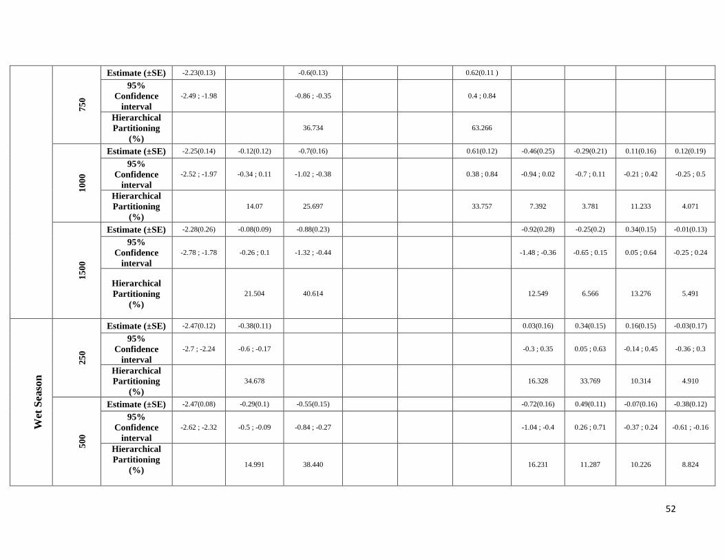
52

75

0

Estimate (±SE) -2.23(0.13) -0.6(0.13) 0.62(0.11 )

95%

Confidence

interval

-2.49 ; -1.98 -0.86 ; -0.35 0.4 ; 0.84

Hierarchical

Partitioning

(%)

36.734 63.266

10

00

Estimate (±SE) -2.25(0.14) -0.12(0.12) -0.7(0.16) 0.61(0.12) -0.46(0.25) -0.29(0.21) 0.11(0.16) 0.12(0.19)

95%

Confidence

interval

-2.52 ; -1.97 -0.34 ; 0.11 -1.02 ; -0.38 0.38 ; 0.84 -0.94 ; 0.02 -0.7 ; 0.11 -0.21 ; 0.42 -0.25 ; 0.5

Hierarchical

Partitioning

(%)

14.07 25.697 33.757 7.392 3.781 11.233 4.071

15

00

Estimate (±SE) -2.28(0.26) -0.08(0.09) -0.88(0.23) -0.92(0.28) -0.25(0.2) 0.34(0.15) -0.01(0.13)

95%

Confidence

interval

-2.78 ; -1.78 -0.26 ; 0.1 -1.32 ; -0.44 -1.48 ; -0.36 -0.65 ; 0.15 0.05 ; 0.64 -0.25 ; 0.24

Hierarchical

Partitioning

(%)

21.504 40.614 12.549 6.566 13.276 5.491

Wet

Sea

son

25

0

Estimate (±SE) -2.47(0.12) -0.38(0.11) 0.03(0.16) 0.34(0.15) 0.16(0.15) -0.03(0.17)

95%

Confidence

interval

-2.7 ; -2.24 -0.6 ; -0.17 -0.3 ; 0.35 0.05 ; 0.63 -0.14 ; 0.45 -0.36 ; 0.3

Hierarchical

Partitioning

(%)

34.678 16.328 33.769 10.314 4.910

50

0

Estimate (±SE) -2.47(0.08) -0.29(0.1) -0.55(0.15) -0.72(0.16) 0.49(0.11) -0.07(0.16) -0.38(0.12)

95%

Confidence

interval

-2.62 ; -2.32 -0.5 ; -0.09 -0.84 ; -0.27 -1.04 ; -0.4 0.26 ; 0.71 -0.37 ; 0.24 -0.61 ; -0.16

Hierarchical

Partitioning

(%)

14.991 38.440 16.231 11.287 10.226 8.824

53

75

0

Estimate (±SE) -2.47(0.08) -0.33(0.11) -0.42(0.12) -0.65(0.18) 0.61(0.16) -0.21(0.13) -0.5(0.13)

95%

Confidence

interval

-2.63 ; -2.32 -0.54 ; -0.11 -0.66 ; -0.18 -1 ; -0.3 0.3 ; 0.92 -0.47 ; 0.06 -0.76 ; -0.24

Hierarchical

Partitioning

(%)

16.4 49.364 8.130 4.530 11.637 9.939

10

00

Estimate (±SE) -2.48(0.14) -0.33(0.12) -0.64(0.22) 0.51(0.11) -0.95(0.3) 0.38(0.22) -0.31(0.17) -0.45(0.22)

95%

Confidence

interval

-2.76 ; -2.2 -0.56 ;-0.11 -1.07 ;-0.2 0.3 ;0.72 -1.54 ;-0.37 -0.04 ;0.8 -0.64 ;0.02 -0.88 ; -0.01

Hierarchical

Partitioning

(%)

12.107 35.860 31.483 8.419 2.690 8.297 1.140

15

00

Estimate (±SE) -2.48(0.1) 0.53(0.11)

95%

Confidence

interval

-2.68 ;-2.27 0.32 ;0.74

Hierarchical

Partitioning

(%)

100

Rhinophylla pumilio

Local-scale

Compositional Predictors

Configurational Predictors

Season Spatial

Scale (m)

Explanatory

Variables Intercept

Vegetation

structure FC SF 1 SF 2 SF 3 PD ED MNND MSI

Dry

Sea

son

25

0

Estimate (±SE) -3.67(0.19) -0.2(0.08) 0.17(0.07)

95%

Confidence

interval

-4.05 ;-3.29 -0.36 ;-0.04 0.02 ;0.31

Hierarchical

Partitioning

(%)

11.131 88.869

50

0

Estimate (±SE) -3.65(0.18) 0.04(0.1) -0.05(0.11) -0.03(0.12) 0.09(0.1) 0.05(0.12) -0.12(0.12) 0.09(0.11) 0(0.11) -0.03(0.09)

95%

Confidence

interval

-4 ;-3.31 -0.15 ;0.23 -0.27 ;0.16 -0.26 ;0.19 -0.11 ;0.29 -0.18 ;0.29 -0.36 ;0.11 -0.12 ;0.3 -0.21 ;0.2 -0.2 ; 0.14

54

Hierarchical

Partitioning

(%)

23.231 7.261 3.435 5.985 5.977 37.142 7.465 2.406 7.097

75

0

Estimate (±SE) -3.61(0.12) 0.06(0.09) -0.38(0.08) -0.63(0.34) 0.33(0.12) 0.05(0.12) -0.32(0.1)

95%

Confidence

interval

-3.85 ;-3.37 -0.12 ;0.24 -0.54 ;-0.22 -1.3 ;0.04 0.1 ;0.57 -0.2 ;0.29 -0.51 ; -0.12

Hierarchical

Partitioning

(%)

35.171 19.345 14.906 4.305 20.321 5.952

10

00

Estimate (±SE) -3.64(0.17) 0.04(0.1) -0.15(0.11) 0.11(0.17) 0.05(0.1) 0.17(0.12) -0.11(0.12) 0.09(0.14) -0.05(0.11) 0.09(0.09)

95%

Confidence

interval

-3.98 ;-3.3 -0.15 ;0.23 -0.37 ;0.07 -0.22 ;0.44 -0.15 ;0.24 -0.06 ;0.39 -0.35 ;0.14 -0.18 ;0.36 -0.26 ;0.16 -0.09 ; 0.27

Hierarchical

Partitioning

(%)

26.407 11.833 2.051 5.232 11.688 8.394 2.349 31.088 0.958

15

00

Estimate (±SE) -3.6(0.16) -0.18(0.11) 0.16(0.12) 0.2(0.11) 0.13(0.11)

95%

Confidence

interval

-3.91 ;-3.29 -0.41 ;0.04 -0.08 ;0.41 -0.03 ;0.42 -0.08 ;0.35

Hierarchical

Partitioning

(%)

24.175 13.543 35.078 27.204

Wet

Sea

son

25

0

Estimate (±SE) -3.62(0.08) -0.2(0.08) -0.22(0.08) -0.14(0.09) 0.07(0.08) 0.23(0.09)

95%

Confidence

interval

-3.77 ;-3.46 -0.36 ;-0.05 -0.38 ;-0.06 -0.31 ;0.03 -0.09 ;0.23 0.07 ;0.4

Hierarchical

Partitioning

(%)

7.984 19.453 30.208 21.624 20.731

50

0

Estimate (±SE) -3.62(0.08) -0.2(0.08) -0.22(0.08) 0.22(0.08) 0.21(0.08)

95%

Confidence

interval

-3.78 ;-3.46 -0.36 ;-0.05 -0.38 ;-0.06 0.07 ;0.38 0.05 ;0.37

55

Hierarchical

Partitioning

(%)

10.383 17.040 35.161 37.415

75

0

Estimate (±SE) -3.62(0.08) -0.24(0.08)

95%

Confidence

interval

-3.77 ;-3.47 -0.4 ;-0.09

Hierarchical

Partitioning

(%)

100

10

00

Estimate (±SE) -3.62(0.08) -0.25(0.08) 0.23(0.08)

95%

Confidence

interval

-3.77 ;-3.47 -0.4 ;-0.1 0.08 ;0.38

Hierarchical

Partitioning

(%)

73.698 26.302

15

00

Estimate (±SE) -3.62(0.08) -0.23(0.08) 0.21(0.08) 0.24(0.08)

95%

Confidence

interval

-3.77 ;-3.46 -0.39 ;-0.08 0.06 ;0.37 0.08 ;0.4

Hierarchical

Partitioning

(%)

50.263 31.083 18.655

Lophostoma silvicolum

Local-scale

Compositional Predictors

Configurational Predictors

Season Spatial

Scale (m)

Explanatory

Variables Intercept

Vegetation

structure FC SF 1 SF 2 SF 3 PD ED MNND MSI

Dry

Sea

son

25

0

Estimate (±SE) -5.76(0.3) 0.47(0.3) 0.28(0.2) -0.36(0.22) 0.26(0.25) -0.31(0.28)

95%

Confidence

interval

-6.35 ;-5.17 -0.12 ;1.07 -0.11 ;0.66 -0.78 ;0.06 -0.23 ;0.76 -0.86 ;0.23

Hierarchical

Partitioning

(%)

39.627 20.982 25.402 1.585 12.404

56

50

0

Estimate (±SE) -5.96(0.29) 0.14(0.8) -0.45(0.26) -1.11(0.37) 0.89(0.27)

95%

Confidence

interval

-6.52 ;-5.39 -1.43 ;1.71 -0.97 ;0.06 -1.84 ;-0.39 0.35 ; 1.42

Hierarchical

Partitioning

(%)

18.759 11.702 61.324 8.215

75

0

Estimate (±SE) -5.95(0.31) -0.89(0.33)

95%

Confidence

interval

-6.56 ;-5.33 -1.54 ;-0.24

Hierarchical

Partitioning

(%)

100

10

00

Estimate (±SE) -6.03(0.33) -1.08(0.36)

95%

Confidence

interval

-6.68 ;-5.38 -1.79 ;-0.37

Hierarchical

Partitioning

(%)

100

15

00

Estimate (±SE) -5.95(0.3) -0.85(0.28)

95%

Confidence

interval

-6.53 ;-5.37 -1.4 ;-0.31

Hierarchical

Partitioning

(%)

100

Wet

Sea

son

25

0

Estimate

(±SE)* -5.63(0.22) 0.35(0.19) 17.47(32.75) 2.72(5.29) 2.08(6.99) 5.31(17.65)

95%

Confidence

interval*

-6.07 ;-5.19 -0.03 ;0.72 -46.71 ;81.65 -7.65 ;13.09 -11.63 ;15.78 -29.28 ;39.9

Hierarchical

Partitioning

(%)

20.908 24.18 12.12 18.134 24.659

57

50

0

Estimate (±SE) -5.64(0.21) -0.6(0.17)

95%

Confidence

interval

-6.05 ;-5.24 -0.94 ;-0.27

Hierarchical

Partitioning

(%)

100

75

0

Estimate (±SE) -5.67(0.21) -0.63(0.18)

95%

Confidence

interval

-6.09 ;-5.26 -0.98 ;-0.29

Hierarchical

Partitioning

(%)

100

10

00

Estimate (±SE) -5.64(0.21) -0.55(0.16) -0.7(0.22)

95%

Confidence

interval

-6.06 ;-5.22 -0.87 ;-0.24 -1.14 ;-0.26

Hierarchical

Partitioning

(%)

62.453 37.547

15

00

Estimate (±SE) -5.62(0.21) -0.46(0.17) -0.58(0.2) -0.51(0.18)

95%

Confidence

interval

-6.04 ;-5.2 -0.79 ;-0.14 -0.97 ;-0.18 -0.85 ;-0.16

Hierarchical

Partitioning

(%)

33.951 33.360 32.688

Mimon crenulatum

Local-scale

Compositional Predictors

Configurational Predictors

Season Spatial

Scale (m)

Explanatory

Variables Intercept

Vegetation

structure FC SF 1 SF 2 SF 3 PD ED MNND MSI

Dry

Sea

son

25

0

Estimate (±SE) -5.95(0.35) -0.86(0.38)

95%

Confidence

interval

-6.63 ;-5.27 -1.6 ;-0.13

58

Hierarchical

Partitioning

(%)

100

50

0

Estimate (±SE) -5.95(0.38) 0.44(0.27) -0.41(0.31) 0.57(0.25) -0.59(0.32) -0.55(0.38) -0.59(0.35)

95%

Confidence

interval

-6.7 ;-5.2 -0.09 ;0.98 -1.01 ;0.19 0.07 ;1.07 -1.22 ;0.03 -1.29 ;0.2 -1.28 ;0.09

Hierarchical

Partitioning

(%)

26.698 7.417 6.56 31.21 5.392 22.722

75

0

Estimate (±SE) -5.93(0.36) 0.43(0.26 ) -0.49(0.27)

95%

Confidence

interval

-6.64 ;-5.22 -0.09 ;0.94 -1.02 ;0.05

Hierarchical

Partitioning

(%)

48.661 51.339

10

00

Estimate (±SE) -5.91(0.36) 0.41(0.26) -0.47(0.27)

95%

Confidence

interval

-6.61 ;-5.21 -0.1 ;0.91 -0.99 ;0.06

Hierarchical

Partitioning

(%)

48.245 51.755

15

00

Estimate (±SE) -5.92(0.36) 0.47(0.27) -0.5(0.27)

95%

Confidence

interval

-6.62 ;-5.22 -0.06 ;0.99 -1.03 ;0.03

Hierarchical

Partitioning

(%)

48.893 51.107

Wet

Sea

son

25

0

Estimate (±SE) -5.87(0.25) -1.09(0.3) 0.42(0.16) 0.36(0.19)

95%

Confidence

interval

-6.35 ;-5.39 -1.69 ;-0.49 0.12 ;0.73 -0.02 ;0.74

Hierarchical

Partitioning

(%)

50.461 42.023 7.516

59

50

0

Estimate (±SE) -5.75(0.24) 0.62(0.2)

95%

Confidence

interval

-6.22 ;-5.27 0.24 ;1

Hierarchical

Partitioning

(%)

100

75

0

Estimate (±SE) -5.81(0.3) 0.66(0.22) -1.68(0.58) 1.27(0.48) 0.72(0.23) -0.61(0.35)

95%

Confidence

interval

-6.39 ;-5.24 0.24 ;1.09 -2.81 ;-0.55 0.34 ;2.21 0.27 ;1.18 -1.29 ; 0.07

Hierarchical

Partitioning

(%)

41.232 24.726 11.239 17.984 4.818

10

00

Estimate (±SE) -5.8(0.25) 0.72(0.23)

95%

Confidence

interval

-6.29 ;-5.31 0.26 ;1.17

Hierarchical

Partitioning

(%)

100

15

00

Estimate (±SE) -5.78(0.3) 1990.95(779.51) 158.14(144.68) 107.85(152.07) 1788.98(700.55) 0.42(0.33) 0.49(0.27)

95%

Confidence

interval

-6.36 ;-5.2 463.14 ;3518.77 -125.43 ;441.71

-190.21 ;405.91

415.94 ;3162.03 -0.23 ;1.06 -0.05 ;1.03

Hierarchical

Partitioning

(%)

17.994 11.253 17.47 21.297 4.632 27.354

Trachops cirrhosus

Local-scale

Compositional Predictors

Configurational Predictors

Season Spatial

Scale (m)

Explanatory

Variables Intercept

Vegetation

structure FC SF 1 SF 2 SF 3 PD ED MNND MSI

Dry

Sea

son

25

0

Estimate (±SE) -6.05(0.41) 0.54(0.37) -0.78(0.39) -0.36(0.32)

95%

Confidence

interval

-6.85 ;-5.25 -0.18 ;1.26 -1.54 ;-0.02 -0.99 ;0.27

60

Hierarchical

Partitioning

(%)

57.573 16.885 25.542

50

0

Estimate (±SE) -5.87(0.49) 0.54(0.37) -0.35(0.38) 0.56(0.31) -0.36(0.33) 0.35(0.25)

95%

Confidence

interval

-6.83 ;-4.91 -0.18 ;1.26 -1.09 ;0.38 -0.05 ;1.17 -1 ;0.28 -0.14 ; 0.84

Hierarchical

Partitioning

(%)

36.268 24.558 10.102 25.684 3.389

75

0

Estimate (±SE) -5.72(0.38) 0.62(0.15)

95%

Confidence

interval

-6.47 ;-4.97 0.33 ; 0.91

Hierarchical

Partitioning

(%)

100

10

00

Estimate (±SE) -5.97(0.41) 0.54(0.37) 0.53(0.25) -0.6(0.26) 0.46(0.23)

95%

Confidence

interval

-6.77 ;-5.18 -0.18 ;1.26 0.04 ;1.01 -1.1 ;-0.09 0.01 ; 0.9

Hierarchical

Partitioning

(%)

34.728 27.018 23.627 14.627

15

00

Estimate (±SE) -5.93(0.42) 0.61(0.25) -0.61(0.26) 0.56(0.22)

95%

Confidence

interval

-6.75 ;-5.11 0.12 ;1.09 -1.11 ;-0.11 0.13 ; 1

Hierarchical

Partitioning

(%)

38.628 30.812 30.56

Wet

Sea

son

25

0

Estimate (±SE) -5.35 (0.28) 0.47(0.19) -0.51(0.19)

95%

Confidence

interval

-5.89 ;-4.81 0.1 ;0.84 -0.88 ;-0.13

Hierarchical

Partitioning

(%)

49.239 50.761

61

50

0

Estimate (±SE) -5.35(0.24) -0.65(0.19)

95%

Confidence

interval

-5.83 ;-4.87 -1.02 ;-0.29

Hierarchical

Partitioning

(%)

100

75

0

Estimate (±SE) -5.35(0.25) -0.65(0.19)

95%

Confidence

interval

-5.84 ;-4.86 -1.02 ;-0.28

Hierarchical

Partitioning

(%)

100

10

00

Estimate (±SE) -5.37(0.25) -0.66(0.18)

95%

Confidence

interval

-5.86 ;-4.88 -1.02 ;-0.31

Hierarchical

Partitioning

(%)

100

15

00

Estimate (±SE) -5.28(0.19) -0.7(0.16)

95%

Confidence

interval

-5.65 ;-4.91 -1.01 ;-0.39

Hierarchical

Partitioning

(%)

100

Pteronotus parnellii

Local-scale

Compositional Predictors

Configurational Predictors

Season Spatial

Scale (m)

Explanatory

Variables Intercept

Vegetation

structure FC SF 1 SF 2 SF 3 PD ED MNND MSI

Dry

Sea

son

25

0

Estimate (±SE) -4.56(0.24) -0.45(0.15)

95%

Confidence

interval

-5.02 ;-4.09 -0.74 ;-0.16

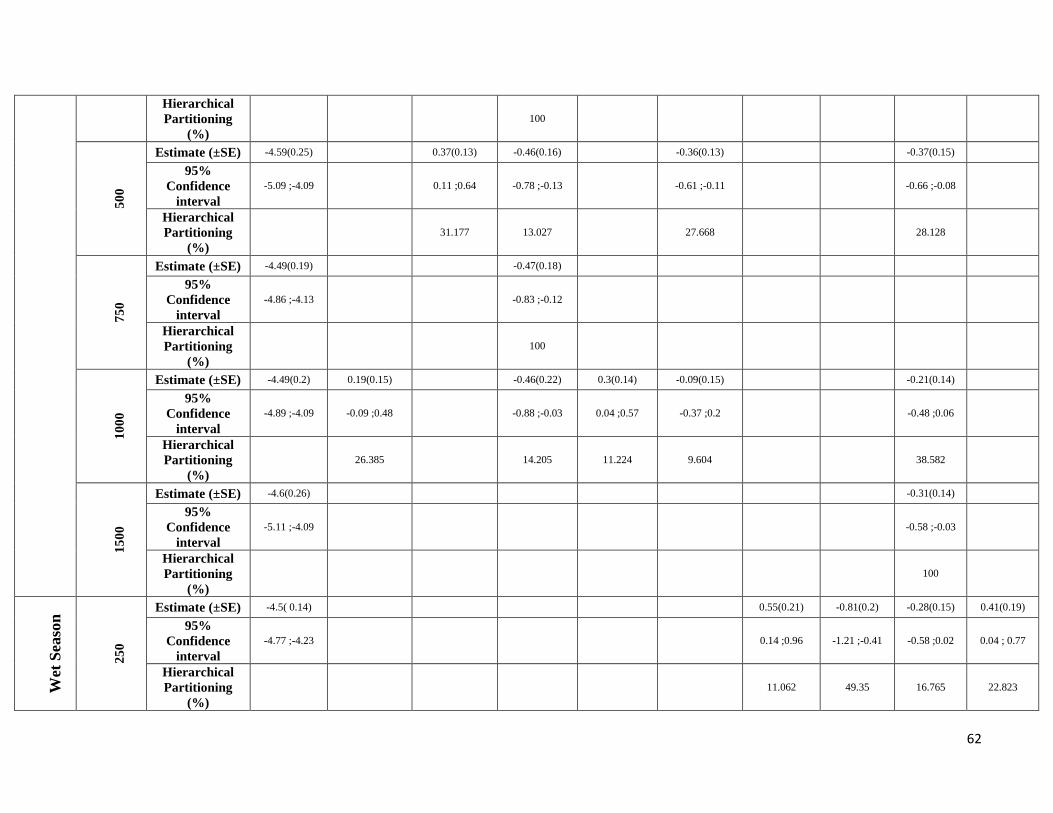
62

Hierarchical

Partitioning

(%)

100

50

0

Estimate (±SE) -4.59(0.25) 0.37(0.13) -0.46(0.16) -0.36(0.13) -0.37(0.15)

95%

Confidence

interval

-5.09 ;-4.09 0.11 ;0.64 -0.78 ;-0.13 -0.61 ;-0.11 -0.66 ;-0.08

Hierarchical

Partitioning

(%)

31.177 13.027 27.668 28.128

75

0

Estimate (±SE) -4.49(0.19) -0.47(0.18)

95%

Confidence

interval

-4.86 ;-4.13 -0.83 ;-0.12

Hierarchical

Partitioning

(%)

100

10

00

Estimate (±SE) -4.49(0.2) 0.19(0.15) -0.46(0.22) 0.3(0.14) -0.09(0.15) -0.21(0.14)

95%

Confidence

interval

-4.89 ;-4.09 -0.09 ;0.48 -0.88 ;-0.03 0.04 ;0.57 -0.37 ;0.2 -0.48 ;0.06

Hierarchical

Partitioning

(%)

26.385 14.205 11.224 9.604 38.582

15

00

Estimate (±SE) -4.6(0.26) -0.31(0.14)

95%

Confidence

interval

-5.11 ;-4.09 -0.58 ;-0.03

Hierarchical

Partitioning

(%)

100

Wet

Sea

son

25

0

Estimate (±SE) -4.5( 0.14) 0.55(0.21) -0.81(0.2) -0.28(0.15) 0.41(0.19)

95%

Confidence

interval

-4.77 ;-4.23 0.14 ;0.96 -1.21 ;-0.41 -0.58 ;0.02 0.04 ; 0.77

Hierarchical

Partitioning

(%)

11.062 49.35 16.765 22.823

63

50

0

Estimate (±SE) -4.5(0.15) 0.4(0.13) -0.4(0.13)

95%

Confidence

interval

-4.79 ;-4.21 0.15 ;0.66 -0.66 ;-0.14

Hierarchical

Partitioning

(%)

53.247 46.753

75

0

Estimate (±SE) -4.5(0.15) 0.4(0.13) -0.4(0.13)

95%

Confidence

interval

-4.79 ;-4.21 0.15 ;0.65 -0.65 ;-0.14

Hierarchical

Partitioning

(%)

54.196 45.804

10

00

Estimate (±SE) -4.49(0.15) 0.38(0.13) -0.38(0.13)

95%

Confidence

interval

-4.78 ;-4.21 0.13 ;0.64 -0.64 ;-0.12

Hierarchical

Partitioning

(%)

54.699 45.301

15

00

Estimate (±SE) -4.49(0.15) 0.38(0.13) -0.37(0.13) -0.35(0.13)

95%

Confidence

interval

-4.78 ;-4.2 0.12 ;0.63 -0.62 ;-0.11 -0.61 ;-0.1

Hierarchical

Partitioning

(%)

33.731 28.076 38.193

64

Table S7. Best-fit models (∆AICc ≤ 2) investigating the relationship between local and landscape-scale attributes and abundance of eight species for the wet

and dry seasons and for five focal scales across the BDFFP, Central Amazon, Brazil. For each model, the number of estimated parameters (K), sample-size

adjusted Akaike’s information criterion (AICc), Akaike differences (Δi), Akaike weights (wi), cumulative Akaike weight (CumW) and log-likelihood (log(L))

are presented. Predictor abbreviations: LVS – local vegetation structure; PFC – primary forest cover; SFC1 – initial secondary forest cover; SFC2 –

intermediate secondary forest cover; SFC3 – advanced secondary forest cover; ED – edge density; PD – patch density; MNND – mean nearest neighbour

distance; MSI – mean shape index;

Artibeus obscurus

Season Spatial Scale (m) Model structure K AICc Δi wi Cum log(L)

Dry

Sea

son

250

SFC1 4 137.20 0 0.28 0.28 -64.01

LVS+SFC1+SFC2+SFC3+ED+PD+MNND+MSI 11 138.98 1.78 0.12 0.40 -53.60

ED 4 139.01 1.81 0.11 0.51 -64.92

PD 4 139.09 1.89 0.11 0.62 -64.96

50

0

SFC3 4 139.14 0 0.20 0.20 -64.98

LVS 4 139.39 0.25 0.17 0.37 -65.11

PFC 4 139.41 0.27 0.17 0.55 -65.12

SFC1 4 140.91 1.76 0.08 0.63 -65.87

750

SFC3 4 138.10 0 0.30 0.30 -64.46

65

PFC 4 139.32 1.22 0.16 0.46 -65.07

LVS 4 139.39 1.29 0.16 0.62 -65.11

1000

SFC3 4 138.19 0 0.22 0.22 -64.51

SFC1+SFC2+SFC3 6 138.84 0.65 0.16 0.38 -62.11

LVS 4 139.39 1.20 0.12 0.50 -65.11

PD 4 139.53 1.34 0.11 0.61 -65.17

PFC 4 139.80 1.61 0.10 0.71 -65.31

1500

SFC1+SFC2+SFC3 6 132.84 0 0.52 0.52 -59.11

Wet

Sea

son

25

0

SFC2 4 100.74 0 0.24 0.24 -45.78

LVS 4 101.21 0.46 0.19 0.43 -46.02

PFC 4 101.31 0.57 0.18 0.61 -46.07

SFC1 4 102.06 1.32 0.12 0.73 -46.44

SFC3 4 102.73 1.99 0.09 0.82 -46.78

500

PD 4 100.12 0 0.29 0.29 -45.47

LVS 4 101.21 1.09 0.17 0.46 -46.02

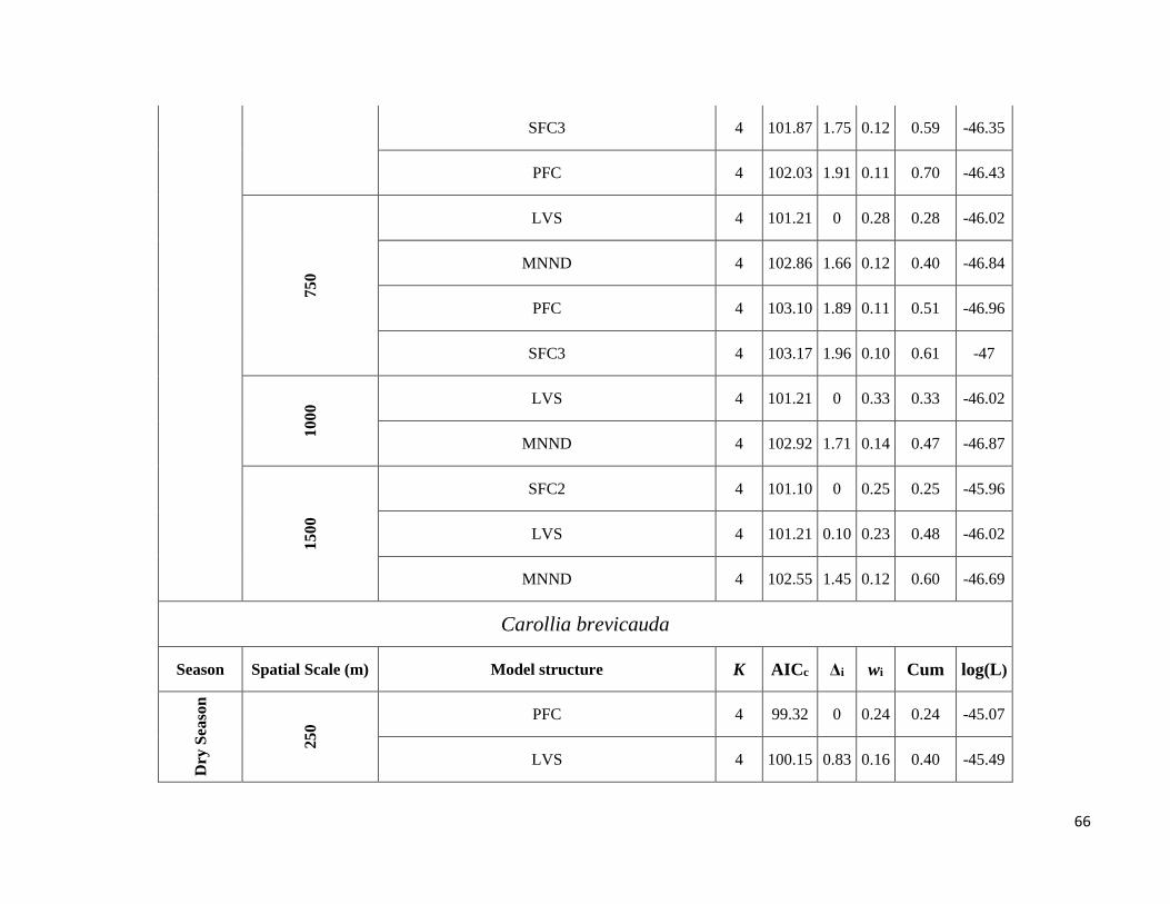
66

SFC3 4 101.87 1.75 0.12 0.59 -46.35

PFC 4 102.03 1.91 0.11 0.70 -46.43

750

LVS 4 101.21 0 0.28 0.28 -46.02

MNND 4 102.86 1.66 0.12 0.40 -46.84

PFC 4 103.10 1.89 0.11 0.51 -46.96

SFC3 4 103.17 1.96 0.10 0.61 -47

1000 LVS 4 101.21 0 0.33 0.33 -46.02

MNND 4 102.92 1.71 0.14 0.47 -46.87

15

00

SFC2 4 101.10 0 0.25 0.25 -45.96

LVS 4 101.21 0.10 0.23 0.48 -46.02

MNND 4 102.55 1.45 0.12 0.60 -46.69

Carollia brevicauda

Season Spatial Scale (m) Model structure K AICc Δi wi Cum log(L)

Dry

Sea

son

250

PFC 4 99.32 0 0.24 0.24 -45.07

LVS 4 100.15 0.83 0.16 0.40 -45.49

67

SFC3 4 100.60 1.27 0.13 0.53 -45.71

LVS+ED+PD+MNND+MSI 8 100.85 1.53 0.11 0.65 -40.03

ED 4 101.19 1.87 0.10 0.74 -46.01

500

LVS 4 100.15 0 0.31 0.31 -45.49

PFC 4 100.57 0.42 0.25 0.56 -45.70

SFC3 4 101.04 0.89 0.20 0.76 -45.93

750

LVS 4 100.15 0 0.32 0.32 -45.49

SFC3 4 100.80 0.65 0.23 0.55 -45.81

PFC 4 101.71 1.55 0.15 0.70 -46.27

10

00

LVS 4 100.15 0 0.24 0.24 -45.49

LVS+PFC+ED+PD+MNND+MSI 9 100.53 0.38 0.20 0.44 -38.16

SFC3 4 101.48 1.33 0.12 0.56 -46.15

15

00 ED+PD+MNND+MSI 7 90.59 0 0.47 0.47 -36.49

LVS+ED+PD+MNND+MSI 8 90.79 0.20 0.42 0.89 -35

Wet

Sea

so

n

250

SFC3 4 165.50 0 0.39 0.39 -78.16

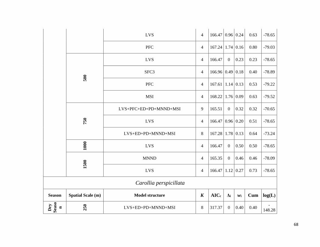
68

LVS 4 166.47 0.96 0.24 0.63 -78.65

PFC 4 167.24 1.74 0.16 0.80 -79.03

500

LVS 4 166.47 0 0.23 0.23 -78.65

SFC3 4 166.96 0.49 0.18 0.40 -78.89

PFC 4 167.61 1.14 0.13 0.53 -79.22

MSI 4 168.22 1.76 0.09 0.63 -79.52

750

LVS+PFC+ED+PD+MNND+MSI 9 165.51 0 0.32 0.32 -70.65

LVS 4 166.47 0.96 0.20 0.51 -78.65

LVS+ED+PD+MNND+MSI 8 167.28 1.78 0.13 0.64 -73.24

10

00

LVS 4 166.47 0 0.50 0.50 -78.65

15

00 MNND 4 165.35 0 0.46 0.46 -78.09

LVS 4 166.47 1.12 0.27 0.73 -78.65

Carollia perspicillata

Season Spatial Scale (m) Model structure K AICc Δi wi Cum log(L)

Dry

Sea

so

n

250

LVS+ED+PD+MNND+MSI 8 317.37 0 0.40 0.40 -

148.28

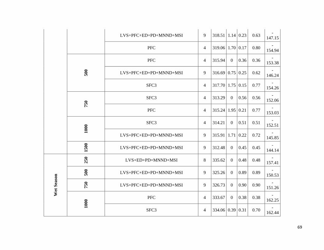
69

LVS+PFC+ED+PD+MNND+MSI 9 318.51 1.14 0.23 0.63 -

147.15

PFC 4 319.06 1.70 0.17 0.80 -

154.94

500

PFC 4 315.94 0 0.36 0.36 -

153.38

LVS+PFC+ED+PD+MNND+MSI 9 316.69 0.75 0.25 0.62 -

146.24

SFC3 4 317.70 1.75 0.15 0.77 -

154.26 750

SFC3 4 313.29 0 0.56 0.56 -

152.06

PFC 4 315.24 1.95 0.21 0.77 -

153.03

1000 SFC3 4 314.21 0 0.51 0.51

-

152.51

LVS+PFC+ED+PD+MNND+MSI 9 315.91 1.71 0.22 0.72 -

145.85

15

00

LVS+PFC+ED+PD+MNND+MSI 9 312.48 0 0.45 0.45 -

144.14

Wet

Sea

son

25

0

LVS+ED+PD+MNND+MSI 8 335.62 0 0.48 0.48 -

157.41

50

0

LVS+PFC+ED+PD+MNND+MSI 9 325.26 0 0.89 0.89 -

150.53

75

0

LVS+PFC+ED+PD+MNND+MSI 9 326.73 0 0.90 0.90 -

151.26

1000 PFC 4 333.67 0 0.38 0.38

-

162.25

SFC3 4 334.06 0.39 0.31 0.70 -

162.44

70

LVS+PFC+ED+PD+MNND+MSI 9 334.98 1.31 0.20 0.90 -

155.39

1500

SFC3 4 332.67 0 0.52 0.52 -

161.75

Rhinophylla pumilio

Season Spatial Scale (m) Model structure K AICc Δi wi Cum log(L)

Dry

Sea

son

250

SFC1 4 193.29 0 0.32 0.32 -92.06

ED 4 193.97 0.69 0.23 0.55 -92.40

50

0

PD 4 197.37 0 0.14 0.14 -94.10

SFC2 4 197.67 0.30 0.12 0.26 -94.25

ED 4 197.69 0.32 0.12 0.38 -94.26

PFC 4 198.19 0.82 0.09 0.47 -94.51

SFC3 4 198.21 0.84 0.09 0.56 -94.52

LVS 4 198.22 0.85 0.09 0.65 -94.52

MSI 4 198.30 0.93 0.09 0.74 -94.56

SFC1 4 198.32 0.95 0.09 0.82 -94.57

MNND 4 198.41 1.04 0.08 0.91 -94.62

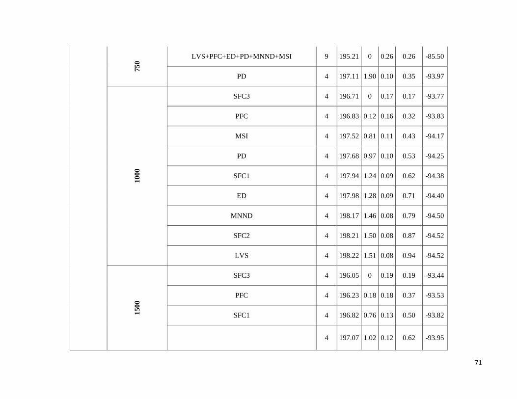
71

75

0 LVS+PFC+ED+PD+MNND+MSI 9 195.21 0 0.26 0.26 -85.50

PD 4 197.11 1.90 0.10 0.35 -93.97

1000

SFC3 4 196.71 0 0.17 0.17 -93.77

PFC 4 196.83 0.12 0.16 0.32 -93.83

MSI 4 197.52 0.81 0.11 0.43 -94.17

PD 4 197.68 0.97 0.10 0.53 -94.25

SFC1 4 197.94 1.24 0.09 0.62 -94.38

ED 4 197.98 1.28 0.09 0.71 -94.40

MNND 4 198.17 1.46 0.08 0.79 -94.50

SFC2 4 198.21 1.50 0.08 0.87 -94.52

LVS 4 198.22 1.51 0.08 0.94 -94.52

15

00

SFC3 4 196.05 0 0.19 0.19 -93.44

PFC 4 196.23 0.18 0.18 0.37 -93.53

SFC1 4 196.82 0.76 0.13 0.50 -93.82

4 197.07 1.02 0.12 0.62 -93.95

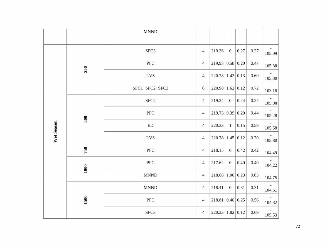
72

MNND

Wet

Sea

son

250

SFC3 4 219.36 0 0.27 0.27 -

105.09

PFC 4 219.93 0.58 0.20 0.47 -

105.38

LVS 4 220.78 1.42 0.13 0.60 -

105.80

SFC1+SFC2+SFC3 6 220.98 1.62 0.12 0.72 -

103.18

500

SFC2 4 219.34 0 0.24 0.24 -

105.08

PFC 4 219.73 0.39 0.20 0.44 -

105.28

ED 4 220.33 1 0.15 0.58 -

105.58

LVS 4 220.78 1.45 0.12 0.70 -

105.80

75

0

PFC 4 218.15 0 0.42 0.42 -

104.49

10

00 PFC 4 217.62 0 0.40 0.40

-

104.22

MNND 4 218.68 1.06 0.23 0.63 -

104.75

1500

MNND 4 218.41 0 0.31 0.31 -

104.61

PFC 4 218.81 0.40 0.25 0.56 -

104.82

SFC3 4 220.23 1.82 0.12 0.69 -

105.53

73

Lophostoma silvicolum

Season Spatial Scale (m) Model structure K AICc Δi wi Cum log(L)

Dry

Sea

son

250

LVS 4 93.09 0 0.22 0.22 -41.96

SFC3 4 93.69 0.60 0.16 0.38 -42.26

MNND 4 94.49 1.39 0.11 0.49 -42.65

PFC 4 94.62 1.53 0.10 0.59 -42.72

ED 4 94.82 1.73 0.09 0.69 -42.82

50

0 ED+PD+MNND+MSI 7 87.20 0 0.45 0.45 -34.79

PD 4 88.84 1.64 0.20 0.64 -39.83

75

0

PD 4 86.46 0 0.64 0.64 -38.64

10

00

PD 4 82.29 0 0.82 0.82 -36.56

1500

PD 4 84.55 0 0.68 0.68 -37.69

Wet

Sea

so

n

250

SFC1+SFC2+SFC3 6 123.40 0 0.21 0.21 -54.39

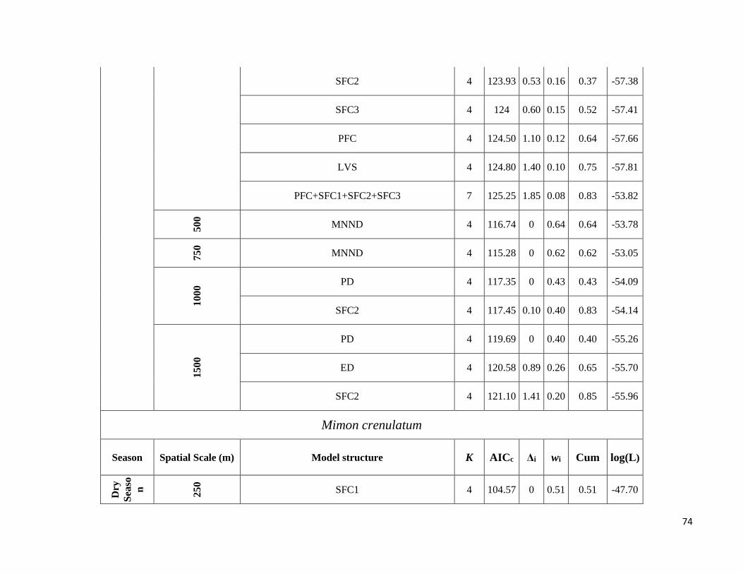
74

SFC2 4 123.93 0.53 0.16 0.37 -57.38

SFC3 4 124 0.60 0.15 0.52 -57.41

PFC 4 124.50 1.10 0.12 0.64 -57.66

LVS 4 124.80 1.40 0.10 0.75 -57.81

PFC+SFC1+SFC2+SFC3 7 125.25 1.85 0.08 0.83 -53.82 500

MNND 4 116.74 0 0.64 0.64 -53.78

750

MNND 4 115.28 0 0.62 0.62 -53.05

1000 PD 4 117.35 0 0.43 0.43 -54.09

SFC2 4 117.45 0.10 0.40 0.83 -54.14

15

00

PD 4 119.69 0 0.40 0.40 -55.26

ED 4 120.58 0.89 0.26 0.65 -55.70

SFC2 4 121.10 1.41 0.20 0.85 -55.96

Mimon crenulatum

Season

Spatial Scale (m) Model structure K AICc Δi wi Cum log(L)

Dry

Sea

so

n

250

SFC1 4 104.57 0 0.51 0.51 -47.70

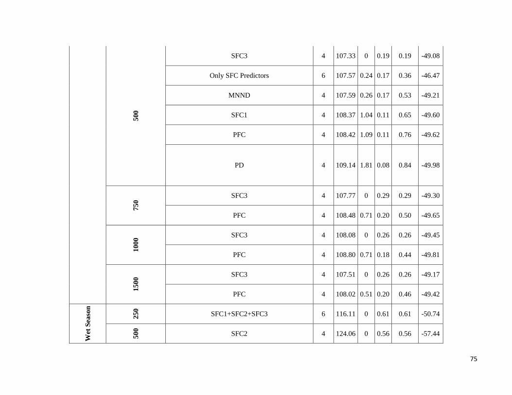
75

500

SFC3 4 107.33 0 0.19 0.19 -49.08

Only SFC Predictors 6 107.57 0.24 0.17 0.36 -46.47

MNND 4 107.59 0.26 0.17 0.53 -49.21

SFC1 4 108.37 1.04 0.11 0.65 -49.60

PFC 4 108.42 1.09 0.11 0.76 -49.62

PD

4 109.14 1.81 0.08 0.84 -49.98

750

SFC3 4 107.77 0 0.29 0.29 -49.30

PFC 4 108.48 0.71 0.20 0.50 -49.65

10

00 SFC3 4 108.08 0 0.26 0.26 -49.45

PFC 4 108.80 0.71 0.18 0.44 -49.81

15

00 SFC3 4 107.51 0 0.26 0.26 -49.17

PFC 4 108.02 0.51 0.20 0.46 -49.42

Wet

Sea

son

25

0

SFC1+SFC2+SFC3 6 116.11 0 0.61 0.61 -50.74

500

SFC2 4 124.06 0 0.56 0.56 -57.44

76

75

0 SFC2 4 123.92 0 0.42 0.42 -57.37

ED+PD+MNND+MSI 7 124.99 1.07 0.25 0.67 -53.69

1000

SFC2 4 123.62 0 0.58 0.58 -57.22

1500

SFC2 4 129.33 0 0.22 0.22 -60.08

MNND 4 129.99 0.66 0.16 0.38 -60.40

PFC+SFC1+SFC2+SFC3 7 130.28 0.95 0.14 0.52 -56.33

ED 4 130.57 1.24 0.12 0.64 -60.70

SFC1 4 131.31 1.98 0.08 0.72 -61.07

Trachops cirrhosus

Season Spatial Scale (m) Model structure K AICc Δi wi Cum log(L)

Dry

Sea

son

25

0

SFC1 4 101.15 0 0.28 0.28 -45.99

LVS 4 101.94 0.79 0.19 0.48 -46.38

MNND 4 103.13 1.98 0.11 0.58 -46.98

500

ED 4 101.68 0 0.21 0.21 -46.25

LVS 4 101.94 0.25 0.18 0.39 -46.38

77

MSI 4 102.55 0.87 0.13 0.52 -46.69

MNND 4 103.30 1.62 0.09 0.62 -47.06

SFC3 4 103.62 1.94 0.08 0.69 -47.22

750

MSI 4 94.89 0 0.71 0.71 -42.86

1000

SFC3 4 100.75 0 0.22 0.22 -45.79

MSI 4 100.94 0.19 0.20 0.42 -45.88

PFC 4 101.60 0.86 0.14 0.57 -46.21

LVS 4 101.94 1.19 0.12 0.69 -46.38

15

00

MSI 4 98.84 0 0.34 0.34 -44.83

PFC 4 100.02 1.17 0.19 0.52 -45.42

SFC3 4 100.28 1.44 0.16 0.69 -45.55

Wet

Sea

son

25

0 SFC3 4 145.85 0 0.39 0.39 -68.34

PFC 4 146.67 0.82 0.26 0.66 -68.75

500

MNND 4 141.63 0 0.70 0.70 -66.23

750

MNND 4 141.45 0 0.73 0.73 -66.14

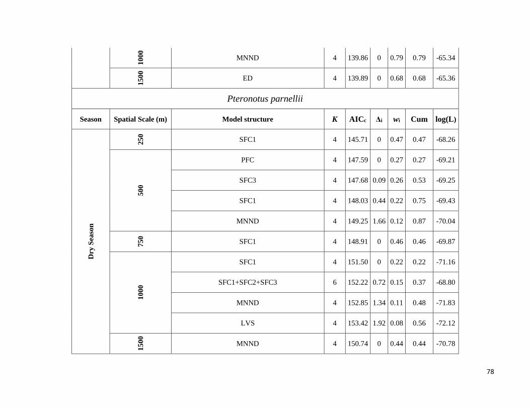
78

10

00

MNND 4 139.86 0 0.79 0.79 -65.34

1500

ED 4 139.89 0 0.68 0.68 -65.36

Pteronotus parnellii

Season Spatial Scale (m) Model structure K AICc Δi wi Cum log(L)

Dry

Sea

son

250

SFC1 4 145.71 0 0.47 0.47 -68.26

500

PFC 4 147.59 0 0.27 0.27 -69.21

SFC3 4 147.68 0.09 0.26 0.53 -69.25

SFC1 4 148.03 0.44 0.22 0.75 -69.43

MNND 4 149.25 1.66 0.12 0.87 -70.04

75

0

SFC1 4 148.91 0 0.46 0.46 -69.87

10

00

SFC1 4 151.50 0 0.22 0.22 -71.16

SFC1+SFC2+SFC3 6 152.22 0.72 0.15 0.37 -68.80

MNND 4 152.85 1.34 0.11 0.48 -71.83

LVS 4 153.42 1.92 0.08 0.56 -72.12

1500

MNND 4 150.74 0 0.44 0.44 -70.78

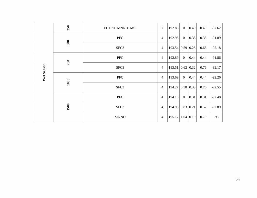
79

Wet

Sea

son

25

0

ED+PD+MNND+MSI 7 192.85 0 0.49 0.49 -87.62

500

PFC 4 192.95 0 0.38 0.38 -91.89

SFC3 4 193.54 0.59 0.28 0.66 -92.18

750

PFC 4 192.89 0 0.44 0.44 -91.86

SFC3 4 193.51 0.62 0.32 0.76 -92.17 1000 PFC 4 193.69 0 0.44 0.44 -92.26

SFC3 4 194.27 0.58 0.33 0.76 -92.55

1500

PFC 4 194.13 0 0.31 0.31 -92.48

SFC3 4 194.96 0.83 0.21 0.52 -92.89

MNND 4 195.17 1.04 0.19 0.70 -93

80

Table S8.Results of the model consistency between dry and wet season for bat-landscape relationships.

Species Model Consistency (%)

Artibeus obscurus 0

Carollia brevicauda 71.43

Carollia perspicillata 71.43

Rhinophylla pumilio 25

Lophostoma silvicolum 40

Mimon crenulatum 28.57

Trachops cirrhosus 33.33

Pteronotus parnellii 37.50