[1]

Effects of Soil-Foundation-Structure Interaction on Seismic Structural Response via Robust

Monte Carlo Simulation

M. Moghaddasi K.1

*, M. Cubrinovski1, J.G. Chase2, S. Pampanin1, A. Carr1

1 Department of Civil and Natural Resources Engineering, University of Canterbury, Private Bag 4800, Christchurch 8140, New Zealand, Tel. (+64) 3-364-2250

2 Mechanical Engineering Department, University of Canterbury, Private Bag 4800,

Christchurch 8140, New Zealand, Tel. (+64) 3-364-2596

For the definitive version, see:

Moghaddasi, M., Cubrinovski, M., Chase, J.G., Pampanin, S. and Carr, A. (2011) Effects of soil-foundation-structure interaction on seismic structural response via robust Monte Carlo simulation. Engineering Structures, 33(4), 1338-1347. http://dx.doi.org/10.1016/j.engstruct.2011.01.011 .

ABSTRACT

Uncertainties involved in the characterization and seismic response of soil-foundation-

structure systems along with the inherent randomness of the earthquake ground motion

result in very complex (and often controversial) effects of soil-foundation-structure

interaction (SFSI) on the seismic response of structures. Conventionally, SFSI effects

have been considered beneficial (reducing the structural response), however, recent

evidence from strong earthquakes has highlighted the possibility of detrimental effects

or increase in the structural response due to SFSI. This paper investigates the effects of

1 Corresponding author. Tel. (+64) 3-364-2250. E-mail address: masoud.moghaddasi@pg.canterbury.ac.nz

[2]

SFSI on seismic response of structures through a robust Monte Carlo simulation using a

wide range of realistic SFS systems and earthquake input motions in time-history

analyses. The results from a total of 1.36 million analyses are used to rigorously

quantify the SFSI effects on structural distortion and total horizontal displacement of

the structure, and to identify conditions (system properties and earthquake motion

characteristics) under which SFSI increases the structural response.

Keywords: Monte Carlo simulation, Soil-foundation-structure interaction, Equivalent

linear model, Ground motion, Uncertainties

1 INTRODUCTION

The complexity of the seismic soil-foundation-structure interaction (SFSI) problem

accompanied with the inherent uncertainty in SFS system parameters and earthquake

motion characteristics has resulted in somewhat controversial interpretation of SFSI

effects on the structural seismic response. Traditionally, the effects of inertial SFSI are

explained by a period lengthening and increased damping of the system [1]-[3], and on

this basis, it has been concluded and implemented in design codes [4],[5] that including

SFSI in the analysis has a beneficial effect (or reduction) in the seismic response of

structures. However, it has been also argued that the perceived beneficial role of SFSI is

an oversimplification of the reality and indeed is incorrect for certain soil-structure

systems and earthquake motions [6]-[10]. In addition, it has been recently shown that

uncertainties arise from structural and geotechnical properties as well as input loading

play an important role in performance prediction of seismically excited structures [11]-

[13]. In particular, for systems considering soil-structure interaction, the effect of

uncertainty on structural demand is even more pronounced [14]-[18].

[3]

In this context, the current study presents an effort for a comprehensive and systematic

investigation of the effects of SFSI on the seismic response of structures. A robust

statistical analysis utilizing Monte Carlo simulation was conducted using idealized soil-

shallow foundation-structure models following the current design practice [19].

Emphasis was given to a random selection of model parameters in a typical SFS system,

such that a wide range of soil, foundation and structural properties were considered and

a large number of widely varying but representative and realistic SFS models were

generated. In these models, the superstructure is assumed to be a linear single-degree-

of-freedom (SDOF) system with 5% equivalent viscous damping. The reasons behind

choosing a linear structural model were: (i) to follow the approach that has been adopted

in building codes for developing design spectrum and defining the seismic forces acting

on the structure; and (ii) to systematically address the problem and evaluate the SFSI

effects, starting with a more simple linear behaviour. Note that in the second phase of

this study which is reported elsewhere [20], the SFSI effects on structural nonlinear

response were considered. The soil-foundation part is represented by an equivalent

linear cone model [21] taking into account nonlinearity in the soil stress-strain

behaviour via the equivalent linear approach [22]. It should be acknowledged that the

adopted soil-foundation element does not cover the extreme material nonlinearity or

geometrical nonlinearity (uplift or sliding) since they are beyond the scope of this study.

The generated SFS models were excited by an ensemble of 40 earthquake ground

motions recorded on stiff/soft soils to account for variability in the input motion. Thus

soil, SFS system and earthquake ground motion variability are considered in this study.

The paper first introduces the procedure and criteria for random generation of SFS

models and then presents the results of 1.36 million analyses in terms of different

[4]

probability levels including the median response and related dispersion. Using

appropriate statistics, the probability for an increase in the structural response or

detrimental effects due to SFSI effects is quantified across wide range of predominant

periods and ground motion characteristics. The correlation between detrimental SFSI

effects and system parameters or ground motion characteristics is also examined and

quantified, and on this basis conditions for detrimental SFSI scenarios are identified.

Respecting the scope of this robust probabilistic study, the presented outcomes are

limited to a SDOF system as a first step in the evaluation of the SSI effects. Also note

the study does not consider extreme conditions such as those imposed by very soft

(liquefiable) soils or near-fault effects on the ground motion.

2 METHODOLOGY FOR MONTE CARLO SIMULATION

The key objective in the Monte-Carlo simulation was to examine the seismic response

of a large number of realistic SFS models when subjected to various earthquake

excitations, and in this way to create basis for quantification of the SFSI effects on the

structural response. Details of the adopted methodology are elaborated in the following

sections.

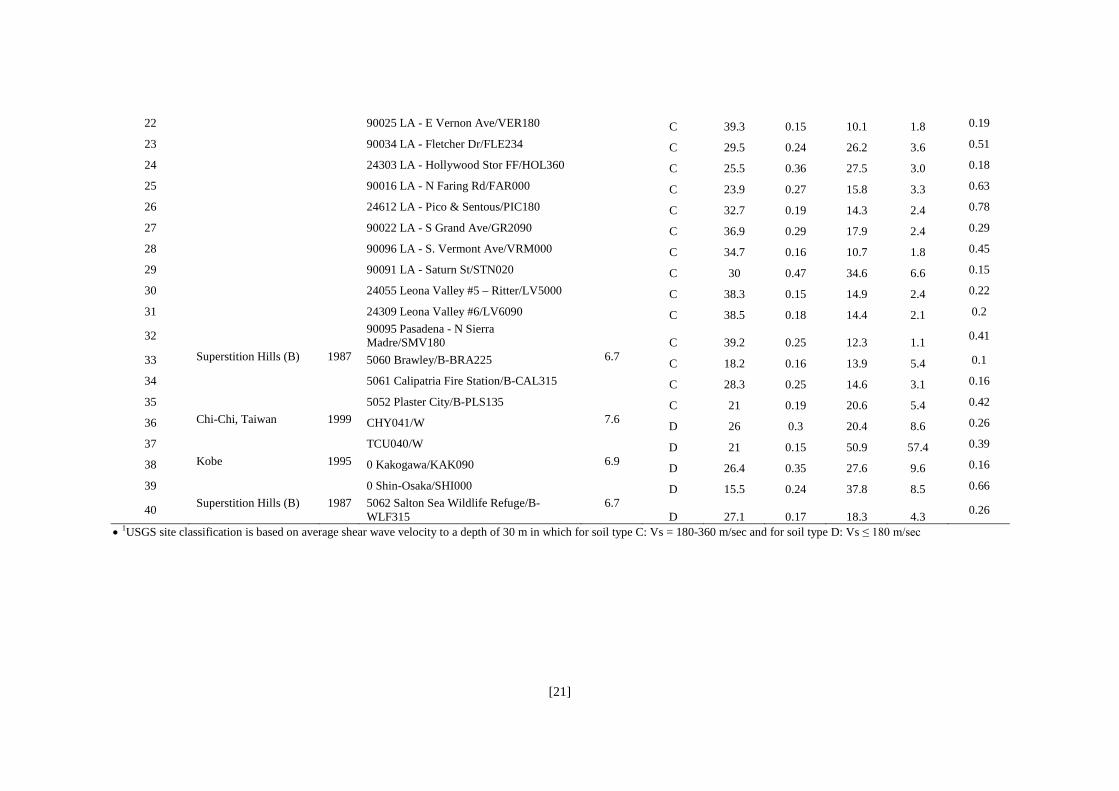
2.1 Adopted soil-shallow foundation-structure model

A fairly simple SFS model was adopted for dynamic time-history analysis to represent

the inertial SFSI effects on structural seismic response. The model consists of a SDOF

system representing a linear superstructure and a set of equivalent linear springs and

dashpots representing the soil-shallow foundation system, as shown in Figure 1. Herein,

only horizontal and rocking motions of the foundation were considered and since the

foundation is located on the ground surface, the horizontal and rocking degrees of

[5]

freedom were modelled independently. As another reasonable simplification, the mass

of the foundation and the mass moment of inertia of the superstructure were neglected

[23].

The idealized SDOF can be interpreted as an equivalent representation of the

fundamental mode of vibration of a fixed-base (FB) multi-storey structure. This SDOF

structural representation is characterized by: (i) structural mass participating in the

fundamental mode of vibration, mstr, (ii) structural lateral stiffness, kstr, (iii) 5%

equivalent viscous structural damping, ξ, and (iv) effective height considered from the

foundation level to the centre of the structural mass, heff. The soil-foundation element is

based on the cone model [21] with frequency-independent coefficients, and it represents

a shallow foundation with a radius, r, resting on a homogeneous linear elastic half-

space. Soil material damping is also considered herein by making use of the classical

Voigt model of viscoelasticity and an equivalent material damping ξ0 which is

compatible with the shear strains induced in the soil. All the coefficients of the applied

soil-foundation element are summarized in Table 1.

To incorporate soil nonlinearity into the adopted soil-foundation element in a simplified

manner, the conventional equivalent linear method was utilized. This approach is based

on representing the soil nonlinearity by using a reduced soil modulus (secant stiffness)

and an increased (equivalent) damping in accordance with the strain level in the ground

induced by the earthquake. As shown in Figure 2, using the equivalent linear approach,

the nonlinear stress-strain curve and corresponding hysteretic damping at a given shear

strain level, γ, are represented by a degraded secant stiffness, Gsec, and an equivalent

viscous damping, ξeq. For a given γ, the value of Gsec is simply evaluated using an

appropriate modulus reduction curve and a known initial shear modulus, Gmax ( Figure

[6]

2b). Similarly, ξeq is read from the respective damping curve (Figure 2c). Through

applying Gsec and respective shear wave velocity, Vsec=(Gsec/ρ)1/2, and ξeq in the adopted

linear soil-foundation element (expressions in Table 1), the stiffness degradation and

damping increase due to the soil nonlinear behaviour was incorporated.

For the purpose of this study, the response of the superstructure was examined using

two response parameters: (i) structural distortion, u, and (ii) structural total

displacement, ustr. Structural distortion is the horizontal displacement of the structure

relative to the foundation; while structural total displacement is the sum of the

horizontal foundation displacement, the structural lateral displacement due to

foundation rocking and the structural distortion.

The combined effect of structural and soil parameters was also evaluated through key

SFS system parameters [2],[21],[24]: (i) structural aspect ratio, r/hh~ eff= , structure-

to-soil mass ratio, 3str r/mm~ ρ= , and structure-to-soil stiffness ratio, str eff sh / Vω ω= ,

(where ωstr is circular frequency of the fixed-base superstructure).

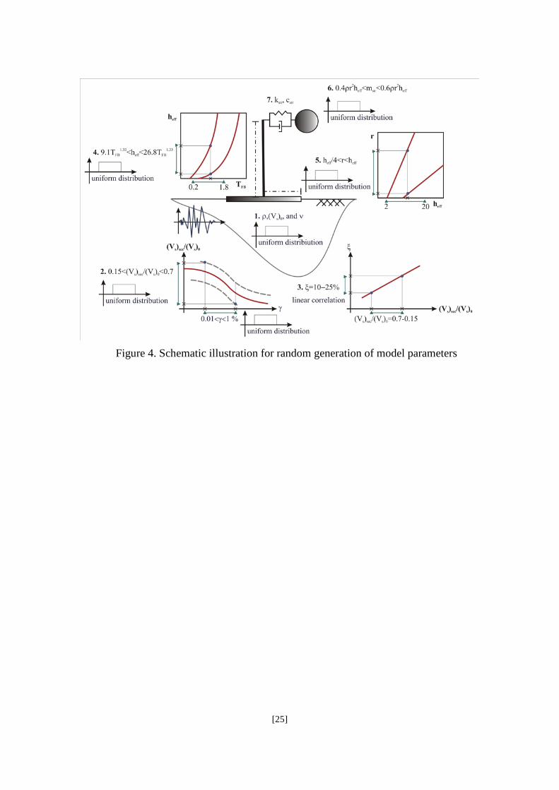
2.2 Generating the random SFS models

SFS models with randomly generated parameters were developed utilizing the

following steps:

(i) Seventeen groups of SFS models were defined, each having a different

predominant period for the FB superstructure, TFB, in the range between 0.2-1.8 sec

at an increment of ΔT=0.1 sec. This period set was selected to present

superstructures with a height of 3-30 m and also satisfy the period-height relationship

specified in the New Zealand Standard (NZS1170.5) [25]. The advantage of

classifying the models in groups with different fundamental periods is that it allows

[7]

to present SFSI effects on structural seismic response in a design spectrum format,

similar to the approach that is followed in design spectrum analysis.

(ii) For each of these 17 groups, 1000 models were randomly generated under

constraints to conform to the adopted TFB and to produce realistic SFS models. The

selection process of the parameters for 1000 models is described below. The number

of 1000 models was chosen with the intention to achieve the best fit distribution for

the randomly selected parameters and increase the accuracy of the Monte-Carlo

simulation [26].

Selection of uncertain soil parameters

Table 2

: With regard to the assumed soil-foundation

element, four main soil parameters were selected as random variables: the initial soil

shear wave velocity, (Vs)0, the shear wave velocity degradation ratio, (Vs)sec/(Vs)0, where

(Vs)sec represents the degraded shear wave velocity, the soil mass density, ρ, and the

Poisson’s ratio, υ. To generate random variables for each parameter, a range of realistic

values was first defined for stiff/soft soils (type C and D based on USGS classification)

and a uniform distribution was assigned to that range. The defined ranges of variation

for all four mentioned soil parameters are summarized in . In this table, the

range of 0.15-0.7 was selected for (Vs)sec/(Vs)0 to represent the expected level of

degradation for an induced shear strain of 0.01-1% in the soil medium. After defining ρ

and (Vs)sec, the degraded shear modulus, Gsec, was calculated:

2secssec )V(G ρ= (1)

To define soil material damping, ξeq, Equation 2 was used. This equation represents the

linear variation of damping between 10-25% corresponding to the velocity degradation

ratio of 0.7-0.15.

[8]

15.07.015.0)V()V(

102525 0ssecseq

−−

=−ξ−

(2)

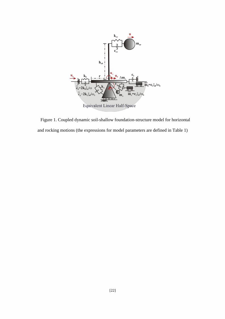
As an example of the adopted distributions used in the analyses, Figure 3a-c illustrates

the distributions of (Vs)sec, Gsec, and ξeq when TFB=1.0 sec.

Selection of realistic structural parameters

Table 3

: The first calculated structural parameter was

the height of the superstructure, heff. The assumed range of variation for heff

(summarized in ) was defined based on: (i) a typical period-height relationship

adopted in NZS 1170.5 [25] that can be expressed in the compact format of:

75.0effFB

75.0eff )h(19.0T)h(085.0 ≤≤ (3)

and (ii) the considered limitation on the structural total height of 3-30 m. For the

defined range, random variables with uniform equal likelihood were selected for each

group of models with a given constant TFB. After defining heff, the building aspect ratio,

r/hh~ eff= , was used to calculate the foundation radius, r. Here, it was assumed that h~

varies from 1-4 for conventional building structures, and also it was assumed that r is

limited to the range of 2-12 m, representing structures having 1-3 bays with length of 4-

8 m each. For each predefined value of heff depending on the criteria introduced in Table

4, a random value was picked for r. For each model, the foundation radius along with

the selected soil parameters was used to calculate the coefficients of the soil-foundation

element. To define a realistic structural mass, mstr, for the defined structural and soil

parameters, relative mass index m was used:

eff2

str

hrmm

ρ= (4)

[9]

Using previously defined values for heff, r and ρ in each group of models with constant

TFB and considering a uniform distribution for m within the range of 0.4-0.6 (an

accepted range for conventional building structures [24],[27]) random values for mstr

were selected. Following this estimation of mstr, the structural lateral stiffness, kstr, and

the structural damping coefficient, cstr, were directly calculated:

str2FB

2

str mT4k π

= (5)

strstrstr mk)05.0(2c = (6)

Figure 3d illustrates the distribution of mstr obtained for TFB=1.0 sec. It is apparent from

Equations 5-6 that the distributions of kstr and cstr will follow the same trend as the

distribution of mstr.

Knowing all the parameters of the model, eventually the predominant period of the SFS

system is calculated:

ϕ

++=khk

kk1TT

2effstr

0

strFBSFS (7)

The described procedure for selection of uncertain soil and structural parameters are

schematically illustrated in Figure 4.

2.3 Performing the Analyses

To cover the aleatory uncertainties caused by record-to-record variability, all the

developed SFS models along with their corresponding FB models were analysed using a

suite of 40 earthquake ground motions. Since kinematic interaction is zero for shallow

[10]

foundation [1],[27], the acceleration time-history of the recorded earthquakes on free-

field was directly used as an input at the foundation level.

Applied input earthquake ground motions

Figure 5

: An ensemble of 40 ground motions recorded

on stiff/soft soils (type C and D based on USGS classification) was used in the analyses

(Table A.1). All the selected records are from earthquakes with magnitude of 6.5-7.5

and have a closest source-to-site distance in the range from 15-40 km. In addition, the

records have peak ground accelerations (PGA) greater than 0.1g. Normalized elastic

acceleration response spectra (for 5% damping) of the selected earthquake records are

shown in .

2.4 Representation of the structural response

Since the considered analyses are equivalent linear, only the maximum values for u

(structural distortion) and ustr (structural total displacement) resulting from the time-

history analyses are discussed. The resulted values for the response of SFS models are

presented in a normalized form as a ratio with respect to the results obtained from the

corresponding FB models for the same earthquake ground motion. Based on these

definitions, SFSI is recognized to have detrimental effects in terms of structural

distortion when uSFS/uFB>1.0 and in terms of structural total displacement when

(ustr)SFS/(ustr)FB>1.0.

2.5 Presentation of results from analyses

To characterize the central tendency of the seismic response of the SFS system, the

median value is selected as the statistical measure. In addition, the level of dispersion

existing in the resulted data in each group of models is quantified in terms of the

coefficient of variation (COV), which is the ratio of the standard deviation to the mean.

[11]

Two alternative approaches are also used to distinguish between the dispersions due to

uncertainty in system parameters (SPs) and record-to-record (RTR) variability. These

two approaches are explained below:

1- COV[E(X|SP): A measure of dispersion in the structural response parameter (X)

due to uncertainty in SPs. To evaluate it, the mean of 40 X values, denoted by

E(X|SP) and resulting from 40 time-history analyses using different input motions,

was calculated first for each of the 1000 adopted models. Afterwards, the COV of

these 1000 calculated mean values is evaluated.

2- COV[E(X|EQ)]: A measure of dispersion in the structural response parameter (X)

due to RTR variability. To calculate it, the mean value of 1000 X values, denoted by

E(X|EQ) and resulting from 1000 time-history analyses over 1000 adopted models,

was calculated first for each of the 40 ground motions. Afterwards, the COV of these

40 calculated mean values is calculated.

3 RESULTS AND DISCUSSION

In this Monte Carlo simulation, the wide range of selected models (2×17000 SFS and

FB models) and ground motions (40 earthquakes) yielded 1.36 million analyses in total.

It thus allows for a comprehensive statistical study of the effects of foundation

flexibility on the structural seismic response. The outcomes from the analyses are

detailed in four sections: (i) quantification of the SFSI effects on structural seismic

response; (ii) evaluation of the risk for having detrimental SFSI effects on structural

seismic response (or DSFSI) and quantification of the corresponding increase in the

structural response; (iii) identification of DSFSI scenarios in terms of earthquake

motion characteristics; and (iv) correlation between the likelihood of DSFSI effects and

key SFS system characteristics.

[12]

3.1 Quantification of the SFSI effects on structural seismic response

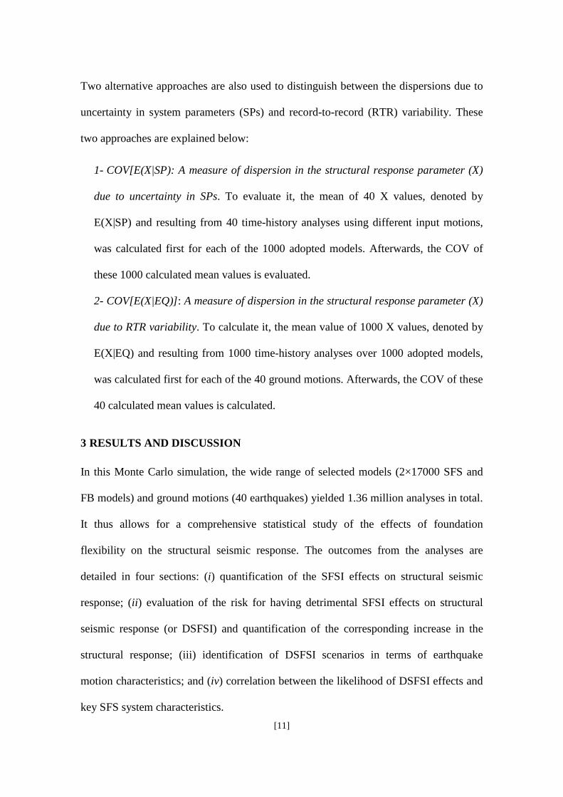
Structural Distortion Figure 6: displays the median and the maximum values of

structural distortion modification factor (uSFS/uFB) in a design spectrum format. At each

specific period, the resulting responses from 40,000 different scenarios (40 earthquakes

and 1000 models) are presented. Clearly, the median response for all considered

scenarios is less than unity, indicating that in 50% of all cases (or on average), SFSI

decreases the deformation of the structure or the drift level. The median values are in

the range of 0.7-0.9 depending on the value of TFB. However, it is evident that for some

cases SFSI may increase the structural distortion and nearly double the response of the

FB model.

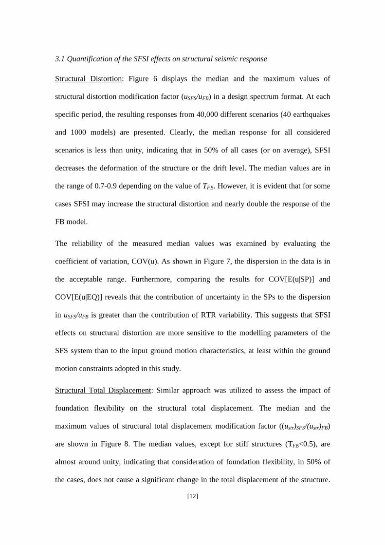
The reliability of the measured median values was examined by evaluating the

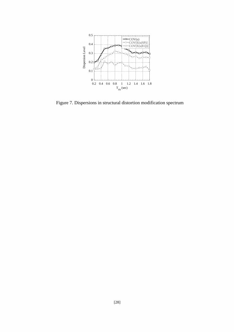
coefficient of variation, COV(u). As shown in Figure 7, the dispersion in the data is in

the acceptable range. Furthermore, comparing the results for COV[E(u|SP)] and

COV[E(u|EQ)] reveals that the contribution of uncertainty in the SPs to the dispersion

in uSFS/uFB is greater than the contribution of RTR variability. This suggests that SFSI

effects on structural distortion are more sensitive to the modelling parameters of the

SFS system than to the input ground motion characteristics, at least within the ground

motion constraints adopted in this study.

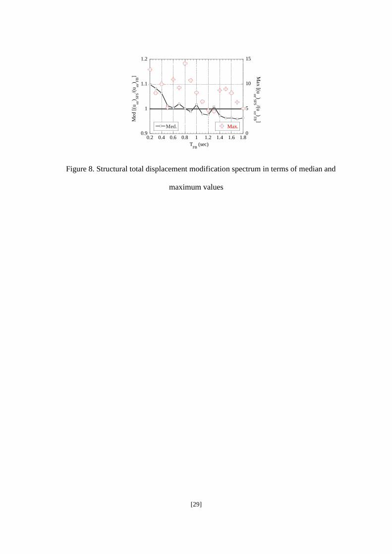
Structural Total Displacement

Figure 8

: Similar approach was utilized to assess the impact of

foundation flexibility on the structural total displacement. The median and the

maximum values of structural total displacement modification factor ((ustr)SFS/(ustr)FB)

are shown in . The median values, except for stiff structures (TFB<0.5), are

almost around unity, indicating that consideration of foundation flexibility, in 50% of

the cases, does not cause a significant change in the total displacement of the structure.

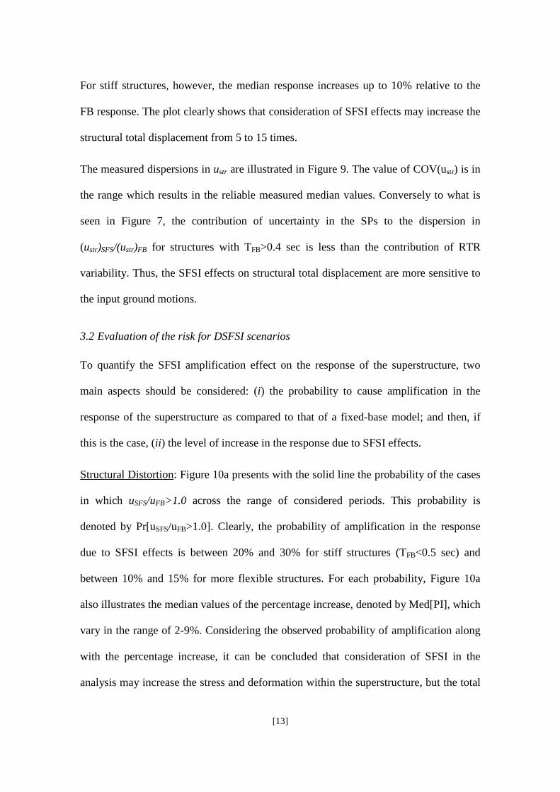
[13]

For stiff structures, however, the median response increases up to 10% relative to the

FB response. The plot clearly shows that consideration of SFSI effects may increase the

structural total displacement from 5 to 15 times.

The measured dispersions in ustr are illustrated in Figure 9. The value of COV(ustr) is in

the range which results in the reliable measured median values. Conversely to what is

seen in Figure 7, the contribution of uncertainty in the SPs to the dispersion in

(ustr)SFS/(ustr)FB for structures with TFB>0.4 sec is less than the contribution of RTR

variability. Thus, the SFSI effects on structural total displacement are more sensitive to

the input ground motions.

3.2 Evaluation of the risk for DSFSI scenarios

To quantify the SFSI amplification effect on the response of the superstructure, two

main aspects should be considered: (i) the probability to cause amplification in the

response of the superstructure as compared to that of a fixed-base model; and then, if

this is the case, (ii) the level of increase in the response due to SFSI effects.

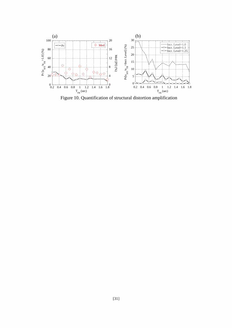
Structural Distortion Figure 10: a presents with the solid line the probability of the cases

in which uSFS/uFB>1.0 across the range of considered periods. This probability is

denoted by Pr[uSFS/uFB>1.0]. Clearly, the probability of amplification in the response

due to SFSI effects is between 20% and 30% for stiff structures (TFB<0.5 sec) and

between 10% and 15% for more flexible structures. For each probability, Figure 10a

also illustrates the median values of the percentage increase, denoted by Med[PI], which

vary in the range of 2-9%. Considering the observed probability of amplification along

with the percentage increase, it can be concluded that consideration of SFSI in the

analysis may increase the stress and deformation within the superstructure, but the total

[14]

risk of an increase in the level of expected damage is relatively low. However, as shown

in Figure 6, there is always a possibility of encountering extreme cases where the

amplification in the response is almost 100%. To better quantify the probability for an

increase in the structural distortion due to SFSI effects, Figure 10b indicates the

probability for amplification of the response of more than 10% and more than 25%

respectively, relative to the fixed-base response. This figure shows that there is a

probability of 2-10% the structural distortion to be increased due to SFSI effects by

more than 10% and a probability of less than 2% the response to be amplified by more

than 25%.

Structural Total Displacement Figure 11: In terms of structural total displacement, a

shows the probability of the cases in which (ustr)SFS/(ustr)FB>1.0. This probability is

denoted by Pr[(ustr)SFS/(ustr)FB>1.0]. For stiffer structures (TFB<0.5 sec), the probability

of having an amplified response due to SFSI consideration is in the range of 50-80%

and this probability reduces to 40-50% for more flexible, longer period, structures. The

median values of the corresponding percentage increase are around 8-18%. However, as

shown in Figure 8, in extreme cases, foundation flexibility may cause an increase in the

structural horizontal displacement by a factor of 15. This amplification is important if

structural pounding is of concern or yielding of foundation soil is expected. Figure 11b

shows that there is a probability of 20-50% for at least 10% increase (or greater) in the

total displacement due to SFSI effects, while there is about 10-30% probability for

amplification of this displacement of over 25%.

3.3 Identification of DSFSI scenarios in terms earthquake motion properties

As demonstrated in Sections 3.1 and 3.2, detrimental SFSI effects are expected to occur

for certain soil-structure systems and earthquake excitations. In this section, the relation

[15]

between the characteristics of the SFS model and the earthquake motion that may cause

an increase in the structural distortion (or strength demand in linear analysis) is

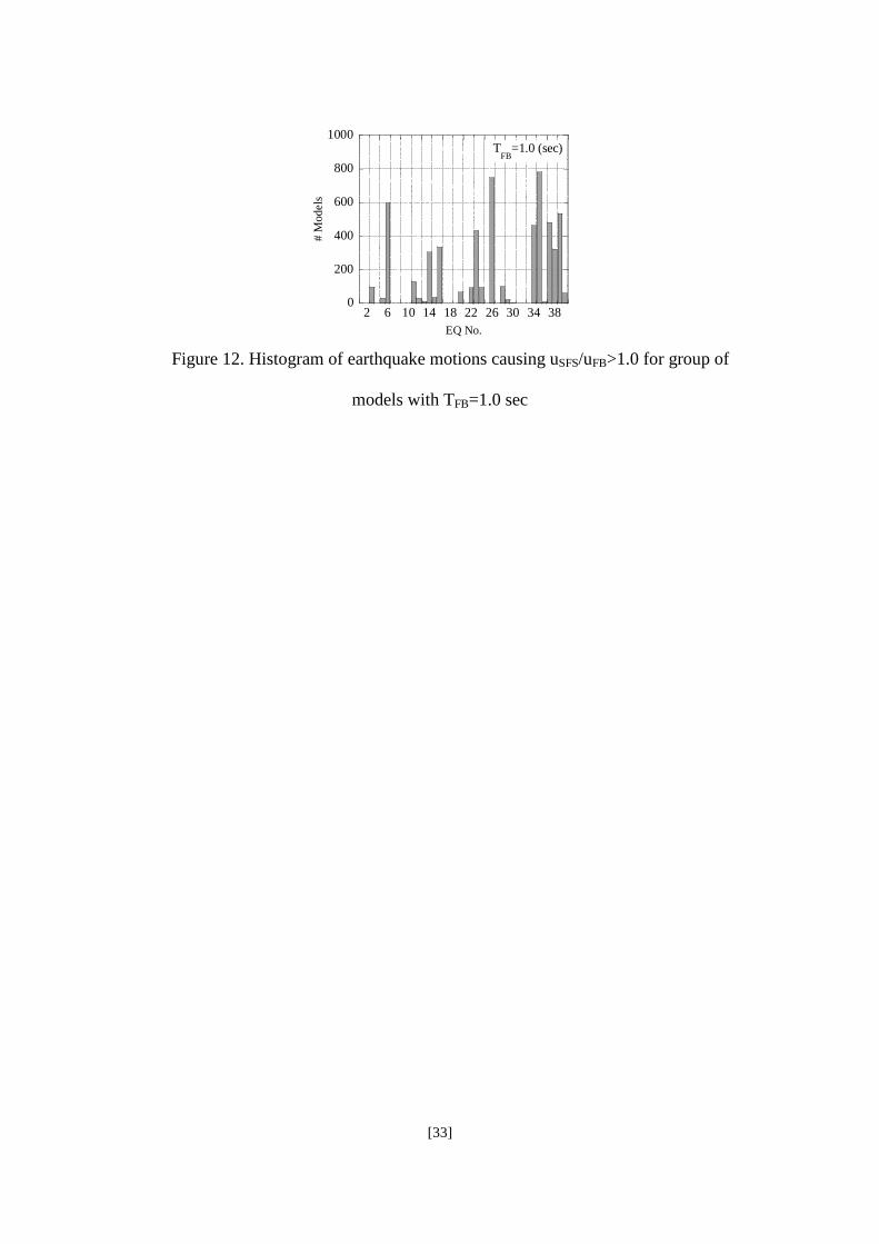
investigated. To illustrate the role of the input motion properties in stimulating DSFSI

scenarios, the histogram of earthquake motions causing detrimental SFSI effects for

models with TFB=1.0 sec is shown in Figure 12, as an example. Clearly, the increase in

the structural distortion depends on the particular ground motion used and is very

pronounced for some earthquakes while completely absent for others. For instance, EQ

No. 23 causes detrimental effects for more than 400 SFS models while EQ No. 2 causes

no detrimental effects at all.

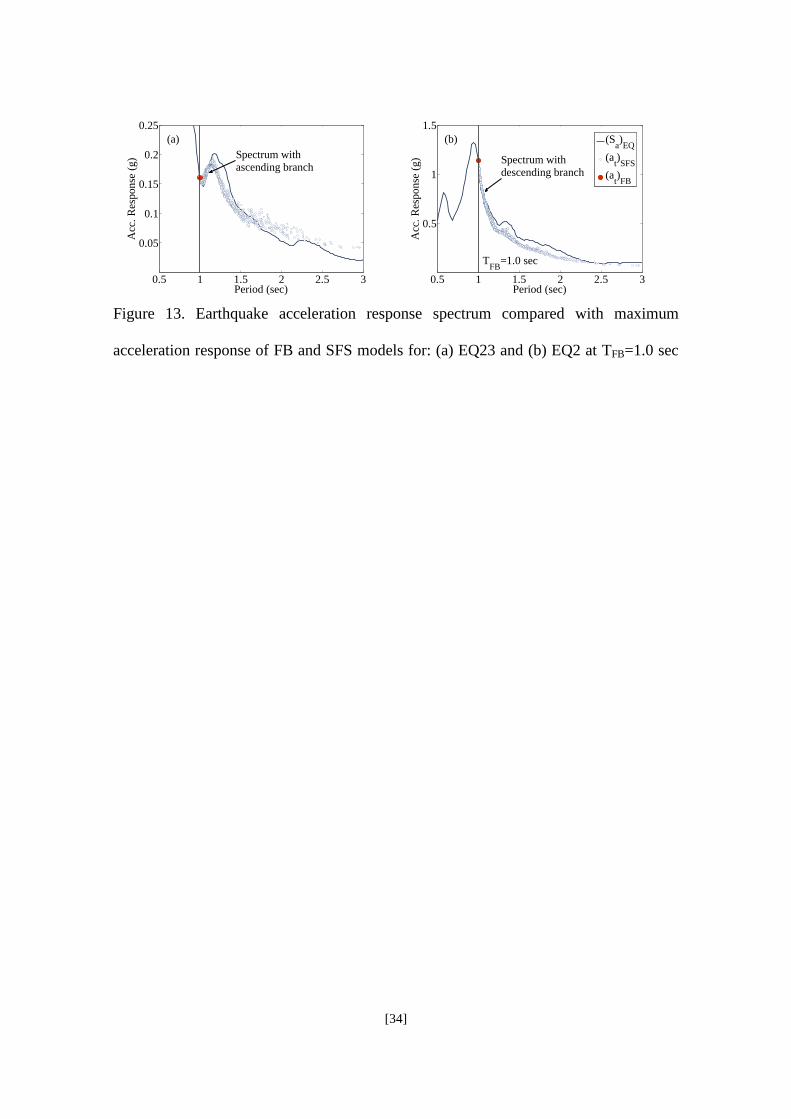
To clarify this outcome, Figures 13a and 13b show with the solid line the acceleration

response spectrum of the earthquake (input) motion, (Sa)EQ, along with the computed

maximum acceleration response of the FB model, (at)FB (shown with the bold symbol),

and SFS models, (at)SFS (open symbols), for systems with TFB=1.0 sec subjected to EQ

No. 23 (Figure 13a) and EQ No. 2 (Figure 13b) respectively. As shown in the figure, the

response pattern of the SFS models closely follows the shape of the response spectrum

of the earthquake motion, though some deviation around the spectrum line is apparent.

This response feature together with the fact that foundation flexibility increases the

period of the system (TSFS > TFB, e.g. Equation 7) leads to a simple rule for

identification of the SFSI effects: SFSI will result in detrimental effects or increase in

the structural response relative to that of the fixed-base model if the response spectrum

of the input earthquake motion has an ascending branch (Figure 13a) in the range of

periods slightly greater than TFB. On the other hand, if the spectrum has a descending

branch in this range of periods, then SFSI effects will be beneficial and will cause a

decrease in the structural response (Figure 13b).

[16]

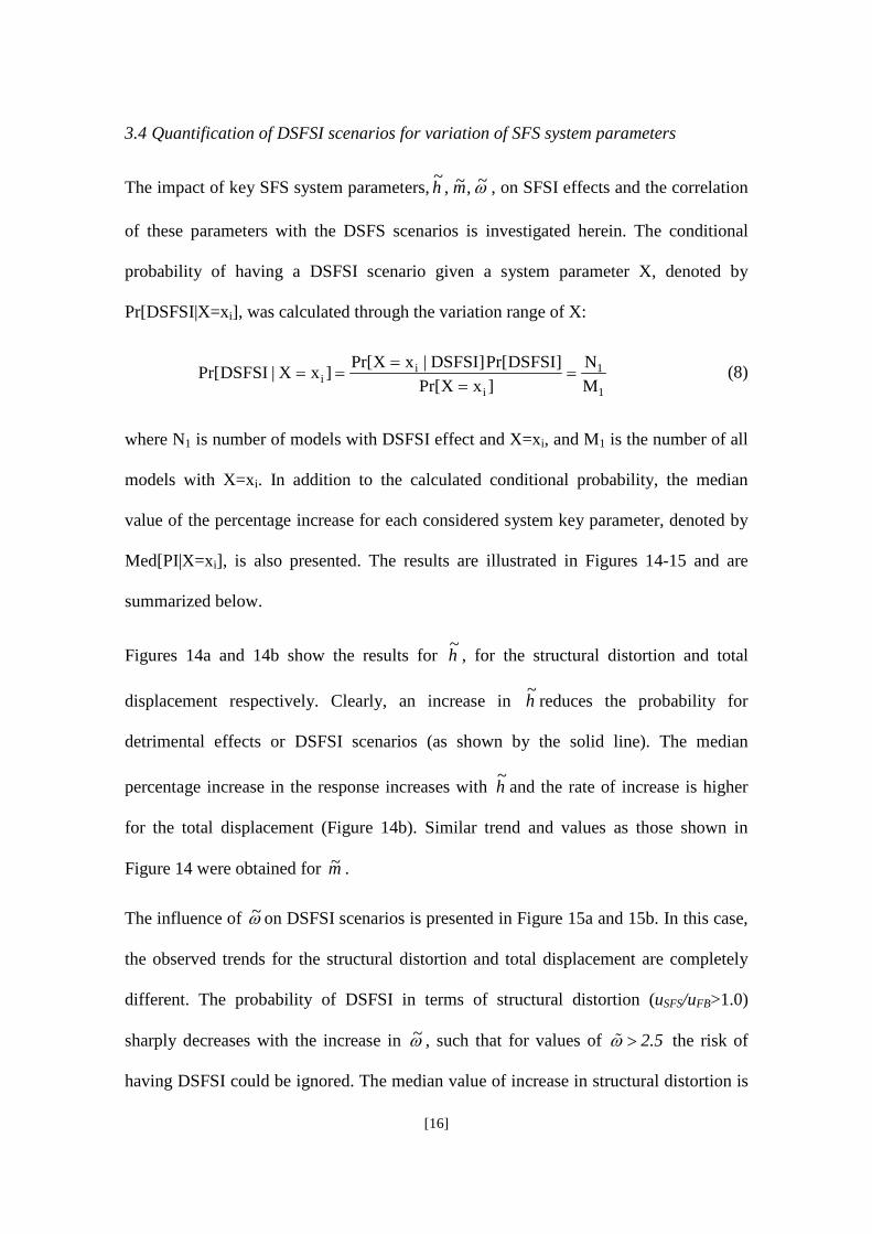
3.4 Quantification of DSFSI scenarios for variation of SFS system parameters

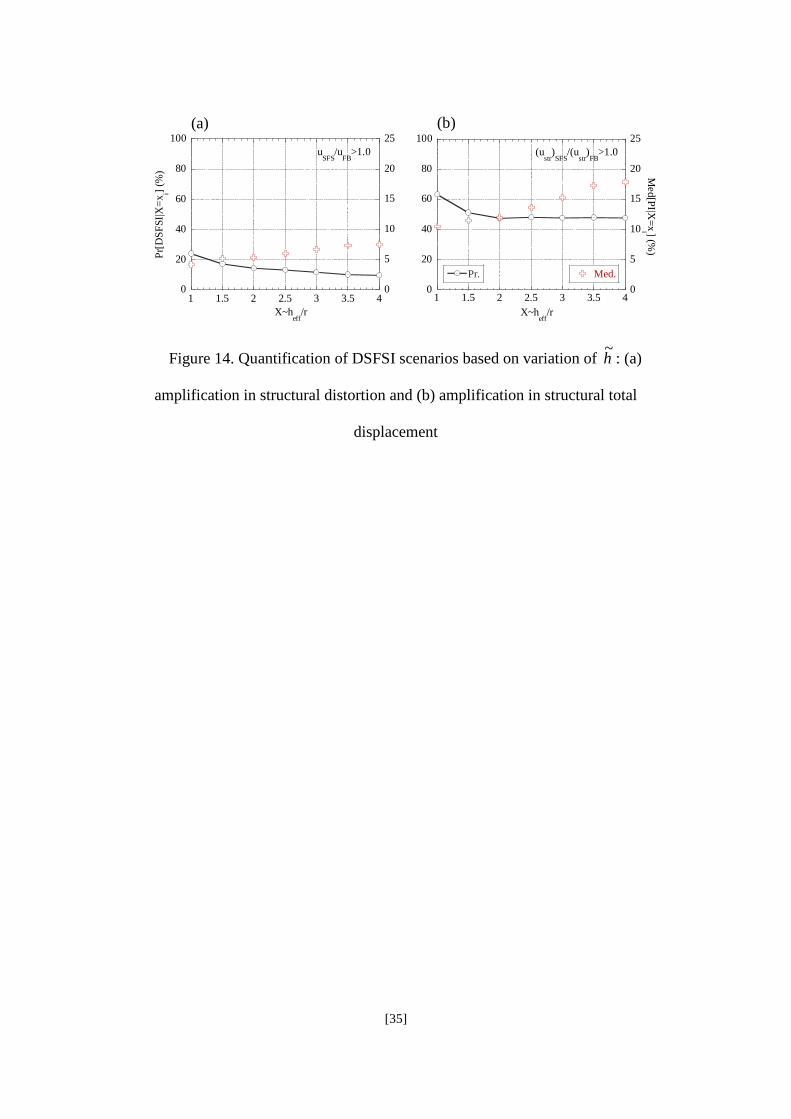
The impact of key SFS system parameters, ω~,m~,h~ , on SFSI effects and the correlation

of these parameters with the DSFS scenarios is investigated herein. The conditional

probability of having a DSFSI scenario given a system parameter X, denoted by

Pr[DSFSI|X=xi], was calculated through the variation range of X:

1

1

i

ii M

N]xXPr[

]DSFSIPr[]DSFSI|xXPr[]xX|DSFSIPr[ ==

=== (8)

where N1 is number of models with DSFSI effect and X=xi, and M1 is the number of all

models with X=xi. In addition to the calculated conditional probability, the median

value of the percentage increase for each considered system key parameter, denoted by

Med[PI|X=xi], is also presented. The results are illustrated in Figures 14-15 and are

summarized below.

Figures 14a and 14b show the results for h~ , for the structural distortion and total

displacement respectively. Clearly, an increase in h~ reduces the probability for

detrimental effects or DSFSI scenarios (as shown by the solid line). The median

percentage increase in the response increases with h~ and the rate of increase is higher

for the total displacement (Figure 14b). Similar trend and values as those shown in

Figure 14 were obtained for m~ .

The influence of ω~ on DSFSI scenarios is presented in Figure 15a and 15b. In this case,

the observed trends for the structural distortion and total displacement are completely

different. The probability of DSFSI in terms of structural distortion (uSFS/uFB>1.0)

sharply decreases with the increase in ω~ , such that for values of 2.5ω > the risk of

having DSFSI could be ignored. The median value of increase in structural distortion is

[17]

about 10% for 8.4~ <ω and 2-6% for 8.4~ >ω (Figure 15a). For the total displacement,

there is no strong correlation between the probability for DSFS scenarios and ω~ ,

however, there is a clear trend for an increase in the amplification of the response with

ω~ , and this increase reaches 60-70% at high ω~ values (Figure 15b).

4 CONCLUSION

A comprehensive Monte Carlo simulation using an established rheological soil-shallow

foundation-structure (SFS) model was carried out to systematically investigate the

effects of SFS interaction on the seismic response of structures. In the analyses, the

superstructure was represented by a linear single-degree-of-freedom (SDOF) system

while the nonlinear stress-strain relationship of the soil was approximated by an

equivalent linear model. The process of random generation of models was designed to

cover a wide range of soil, foundation and superstructure properties and was constrained

to yield realistic and representative soil-foundation-structure systems. To account for

variability in the earthquake excitation, 40 different ground motions were used as input

in the time-history analyses resulting in a comprehensive set of 1.36 million

simulations. The key findings from these analyses can be summarized as follows:

1) In median terms, the consideration of foundation flexibility in the seismic

analysis reduces the structural distortion by a factor (uSFS/uFB) of 0.7-0.9

depending on the fixed-base period of the superstructure. The median value of

the total displacement factor [(ustr)SFS/(ustr)FB] is in the range between 0.95 and

1.1 indicating that on average SFSI increases the total horizontal displacement of

the superstructure.

2) There is 10-30% likelihood of amplification in the structural distortion due to

SFSI effects with the median percentage increase of 2-9% and a potential

[18]

maximum amplification of nearly 100%. The probability for amplification of the

response for more than 10% is 2-10%, while the probability for amplification of

over 25% is less than 2%.

3) There is 10-30% probability for amplification of the total displacement of the

superstructure due to SFSI effects of over 25%. In the extreme case,

consideration of foundation flexibility may result in fifteen times greater total

(horizontal) displacement of the superstructure as compared to that of the fixed

base structure.

4) There is a clear link between the increase in the structural response due to SFSI

effects and the response spectrum characteristics of the earthquake motion.

Detrimental SFSI effects or increase in the structural distortion occur for ground

motions having an ascending branch in the response spectrum in the range of

periods slightly greater than TFB.

5) An increase in the value of the aspect ratio ( h~ ) or the mass ratio ( m~ ) reduces the

probability for detrimental soil-foundation-structure interaction (DSFSI)

scenarios but raises the median increase in the structural response. Both these

trends are well defined but of relatively small magnitude.

6) There is strong correlation between the detrimental SFSI effects and the stiffness

ratio, ω~ . The probability of DSFSI scenarios in terms of structural distortion

decreases sharply with the increase of ω~ , such that for ω~ > 2.5 this probability is

nearly zero. Conversely, the median amplification of the total structural

displacement steadily increases with ω~ up to values of about 60-70% for ω~ > 4.

REFERENCES

[1] Jennings PC, Beilak J. Dynamics of building-soil interaction. B Seismol Soc Am 1973; 63(1):9-48.

[19]

[2] Veletsos AS, Meek JW. Dynamic behaviour of building-foundation systems. Earthq Eng Struct Dyn 1974; 3:121-38.

[3] Veletsos AS, Nair VVD. Seismic interaction of structures on hysteresis foundations. J Struct Div-ASCE 1975; 101:109-129.

[4] Applied Technology Council. Tentative Provisions for the Development of Seismic Regulations for Buildings; ATC-3-06: California, 1984.

[5] FEMA 440. Recommended Improvements of Nonlinear Static Seismic Analysis Procedures. Applied Technology Council: California, 2005.

[6] Beilak J. Dynamic behaviour of structures with embedded foundations. Earthq Eng Struct Dyn 1975; 3:259-274.

[7] Dutta SC, Bhattacharya K, Roy R. Response of low-rise buildings under seismic ground excitation incorporating soil-structure interaction. Soil Dyn and Earthq Eng 2004; 24:893-914.

[8] Gazetas G, Mylonakis G. Seismic soil-structure interaction: new evidence and emerging issues. Geotechnical Earthquake Engineering and Soil Dynamics 3: proceedings of speciality conference. American Society of Civil Engineers 1998; 1119-74.

[9] Mylonakis G, Gazetas G. Seismic soil-structure interaction: beneficial or detrimental. J Earthq Eng 2000; 4(3): 227-301.

[10] Gazetas G, Mylonakis G. Soil-structure interaction effects on elastic and inelastic structures. Proceedings of the fourth international Conference on recent advances in Geotechnical Earthquake Engineering and Soil Dynamics. San Diego, California, March 26-31, 2001.

[11] Mehanny SSF, Ayou AS. Variability in inelastic displacement demands: Uncertainty in system parameters versus randomness in ground records. Eng Struct 2008; 30(4): 1002-1013.

[12] Chaudhuri A, Chakraborty S. Sensitivity evaluation in seismic reliability analysis of structures. Comput. Methods Appl. Mech. Engrg. 2004; 193: 59-68.

[13] Marano GC, Trentadue F, Morrone E, Amara L. Sensitivity analysis of optimum stochastic nonstationary response spectra under uncertain soil parameters. Soil Dyn and Earthq Eng 2008; 28: 1078-1093.

[14] Barcena A, Esteva L. (2007). Influence of dynamic soil-structure interaction on the nonlinear response and seismic reliability of multistorey systems. Earthq Eng Struct Dyn 2007; 36(3): 327-346.

[15] Jin S, Lutes LD, Sarkani S. (2000). Response variability for a structure with soil-structure interactions and uncertain soil properties. Prob Eng Mech 2000; 15(2): 175-183.

[16] Lutes LD, Sarkani S, Jin S. Response variability of an SSI system with uncertain structural and soil properties. Eng Struc 2000, 22(6): 605-620.

[17] Raychowdhury P. Effect of soil parameter uncertainty on seismic demand of low-rise steel buildings on dense silty sand. Soil Dyn and Earthq Eng 2009; 29(10): 1367-1378.

[18] Moghaddasi M, Cubrinovski M, Pampanin S, Carr A, Chase JG. Monte Carlo Simulation of SSI Effects Using Simple Rheological Soil Model. 2009 NZSEE Conference. Christchurch, New Zealand: 3-5 April 2009.

[19] Stewart JP, et al. Revisions to soil-structure interaction procedures in NEHRP design provisions. Earthq Spectra 2003; 19(3): 677-96.

[20] Moghaddasi M, Cubrinovski M, Pampanin S, Carr A, Chase JG. Probabilistic evaluation of soil-foundation-structure interaction effects on seismic structure response. Earthq Eng Struct Dyn 2010. DOI: 10.1002/eqe. 1011.

[21] Wolf JP. Foundation Vibration Analysis Using Simple Physical Model, Englewood Cliffs, NJ: Prentice-Hall, 1994.

[22] Seed HB, Idriss IM. Soil moduli and damping factors for dynamic response analysis. Report EERC 70-10. Earthquake Engineering Research Centre, 1970.

[23] Beilak J. Dynamic response of nonlinear building foundation systems. Earthq Eng Struct Dyn 1978; 7:17-30.

[24] Nakhaei M, Ghanad MA. The Effect of Soil-Structure Interaction on Damage Index of Building. Eng Struct 2008; 30:1491–99.

[25] NZS 1170.5: Structural Design Actions. Part 5: Earthquake Actions. New Zealand; 2004. [26] Fishman, G. S. Monte Carlo: Concepts, Algorithms, and Applications. New York, Springer-Verlag;

1995. [27] Stewart JP, Fenves GL, Seed RB. Seismic soil-structure interaction in buildings: Ι: analytical

aspects. J Geotech Geoenviron 1999; 125(1) 26-37.

[20]

APPENDIX

Table A. 1. Earthquake ground motions recorded on soil type C/D (USGS categorization1) used as input motions in the analyses

ID Event Year Station M Soil R (km) PGA (g) PGV (cm/s)

PGD (cm) Ta (s)

1 Chi-Chi, Taiwan 1999 CHY010/E 7.6 C 25.4 0.23 21.9 11.1 0.27

2 CHY034/N C 20.2 0.31 48.5 16.5 0.94

3 CHY035/W C 18.2 0.25 45.6 12.0 0.87

4 CHY036/W C 20.4 0.29 38.9 21.2 0.53

5 NST/N C 37 0.39 26.9 16.1 0.17

6 Kocaeli, Turkey 1999 Iznik/IZN090 7.4 C 31.8 0.14 28.8 17.4 1.17

7 Landers 1992 22074 Yermo Fire Station /YER270 7.3 C 24.9 0.25 51.5 43.8 0.68

8 Loma Prieta 1989 57066 Agnews State Hospital/AGW000 6.9 C 28.2 0.17 26.0 12.6 0.26

9 57191 Halls Valley/HVR000 C 31.6 0.13 15.4 3.3 0.78

10 1028 Hollister City Hall/HCH090 C 28.2 0.25 38.5 17.8 0.82

11 57382 Gilroy Array #4/G04000 C 16.1 0.42 38.8 7.1 0.44

12 57425 Gilroy Array #7/GMR090 C 24.2 0.32 16.6 3.3 0.44

13 1601 Palo Alto - SLAC Lab/SLC360 C 36.3 0.28 29.3 9.7 0.31

14 47179 Salinas - John & Work/SJW250 C 32.6 0.11 15.7 7.9 0.22

15 1695 Sunnyvale - Colton Ave/ SVL360 C 28.8 0.21 36.0 16.9 0.21

16 Northridge 1994 25282 Camarillo/CMR180 6.7 C 36.5 0.13 10.9 3.5 0.53

17 90053 Canoga Park - Topanga Can/CNP196 C 15.8 0.42 60.8 20.2 0.6

18 24575 Elizabeth Lake/ELI090 C 37.2 0.16 7.3 2.7 0.26

19 90063 Glendale - Las Palmas/GLP177 C 25.4 0.36 12.3 1.9 0.2

20 90054 LA - Centinela St/CEN155 C 30.9 0.47 19.3 3.5 0.16

21 90060 La Crescenta - New York/NYA090 C 22.3 0.18 12.5 1.1 0.46

[21]

22 90025 LA - E Vernon Ave/VER180 C 39.3 0.15 10.1 1.8 0.19

23 90034 LA - Fletcher Dr/FLE234 C 29.5 0.24 26.2 3.6 0.51

24 24303 LA - Hollywood Stor FF/HOL360 C 25.5 0.36 27.5 3.0 0.18

25 90016 LA - N Faring Rd/FAR000 C 23.9 0.27 15.8 3.3 0.63

26 24612 LA - Pico & Sentous/PIC180 C 32.7 0.19 14.3 2.4 0.78

27 90022 LA - S Grand Ave/GR2090 C 36.9 0.29 17.9 2.4 0.29

28 90096 LA - S. Vermont Ave/VRM000 C 34.7 0.16 10.7 1.8 0.45

29 90091 LA - Saturn St/STN020 C 30 0.47 34.6 6.6 0.15

30 24055 Leona Valley #5 – Ritter/LV5000 C 38.3 0.15 14.9 2.4 0.22

31 24309 Leona Valley #6/LV6090 C 38.5 0.18 14.4 2.1 0.2

32 90095 Pasadena - N Sierra Madre/SMV180 C 39.2 0.25 12.3 1.1 0.41

33 Superstition Hills (B) 1987 5060 Brawley/B-BRA225 6.7 C 18.2 0.16 13.9 5.4 0.1

34 5061 Calipatria Fire Station/B-CAL315 C 28.3 0.25 14.6 3.1 0.16

35 5052 Plaster City/B-PLS135 C 21 0.19 20.6 5.4 0.42

36 Chi-Chi, Taiwan 1999 CHY041/W 7.6 D 26 0.3 20.4 8.6 0.26

37 TCU040/W D 21 0.15 50.9 57.4 0.39

38 Kobe 1995 0 Kakogawa/KAK090 6.9 D 26.4 0.35 27.6 9.6 0.16

39 0 Shin-Osaka/SHI000 D 15.5 0.24 37.8 8.5 0.66

40 Superstition Hills (B) 1987 5062 Salton Sea Wildlife Refuge/B-WLF315

6.7 D 27.1 0.17 18.3 4.3 0.26

• 1USGS site classification is based on average shear wave velocity to a depth of 30 m in which for soil type C: Vs = 180-360 m/sec and for soil type D: Vs ≤ 180 m/sec

[22]

Figure 1. Coupled dynamic soil-shallow foundation-structure model for horizontal

and rocking motions (the expressions for model parameters are defined in Table 1)

[23]

Figure 2. Equivalent linear idealization of non-linear soil behaviour: (a) shear stress-

strain behaviour, (b) secant modulus vs. shear strain and (c) equivalent damping vs.

shear strain

[24]

0

40

80

120

31.8 79.1 126 174 221

Num

ber o

f Sam

ples

(Vs)sec

(m/sec)

(a)

0

100

200

300

400

9.2 103 3.3 104 5.6 104 8 104 1 105

Gsec

(kN/m2)

(b)

0

20

40

60

80

0.11 0.14 0.17 0.2 0.23

Num

ber o

f Sam

ples

ξeq

(c)

0

50

100

150

249.6 813 1376 1940 2503m

str (t)

(d)

Figure 3. Distribution of: (a) degraded shear wave velocity, (b) degraded shear

modulus (c) soil material damping and (d) structural mass for TFB=1.0 sec

[25]

Figure 4. Schematic illustration for random generation of model parameters

[26]

0 1 2 3 4 5

1

2

3

4

5

Period (sec)

Sa/P

GA

Median Spectrum

Figure 5. Normalized elastic acceleration response spectra (5% damping) of the

selected earthquake ground motions to PGA=1.0g

[27]

0.6

0.7

0.8

0.9

1

1.1

1.2

0

0.5

1

1.5

2

0.2 0.4 0.6 0.8 1 1.2 1.4 1.6 1.8

Med. Max.M

ed [u

SFS/u

FB] M

ax [uSFS /u

FB ]

TFB

(sec)

Figure 6. Structural distortion modification spectrum in terms of median and

maximum values

[28]

0

0.1

0.2

0.3

0.4

0.5

0.2 0.4 0.6 0.8 1 1.2 1.4 1.6 1.8

COV(u)COV[E(u|SP)]COV[E(u|EQ)]

Dis

pers

ion

Leve

lT

FB (sec)

Figure 7. Dispersions in structural distortion modification spectrum

[29]

0.9

1

1.1

1.2

0

5

10

15

0.2 0.4 0.6 0.8 1 1.2 1.4 1.6 1.8

Med. Max.M

ed [(

u str) SF

S/(ust

r) FB] M

ax [(ustr )SFS /(u

str )FB ]

TFB

(sec)

Figure 8. Structural total displacement modification spectrum in terms of median and

maximum values

[30]

0

0.1

0.2

0.3

0.4

0.5

0.2 0.4 0.6 0.8 1 1.2 1.4 1.6 1.8

COV(ustr

)COV[E(u

str|SP)]

COV[E(ustr

|EQ)]

Dis

pers

ion

Leve

lT

FB (sec)

Figure 9. Dispersions in structural total displacement modification spectrum

[31]

0

20

40

60

80

100

0

4

8

12

16

20

0.2 0.4 0.6 0.8 1 1.2 1.4 1.6 1.8

Pr MedPr

[uSF

S/uFB

>1.0

] (%

)

TFB

(sec)

Med [PI] (%

)

(a)

0

5

10

15

20

25

30

0.2 0.4 0.6 0.8 1 1.2 1.4 1.6 1.8

Incr. Level=1.0Incr. Level=1.1Incr. Level=1.25

TFB

(sec)

Pr[u

SFS/u

FB>I

ncr.

Leve

l] (%

)

(b)

Figure 10. Quantification of structural distortion amplification

[32]

0

20

40

60

80

100

0

5

10

15

20

0.2 0.4 0.6 0.8 1 1.2 1.4 1.6 1.8

Pr Med

Med [PI] (%

)

Pr [(

u str) SF

S/(ust

r) FB>1

.0] (

%)

TFB

(sec)

(a)

0

20

40

60

80

100

0.2 0.4 0.6 0.8 1 1.2 1.4 1.6 1.8

Incr. Level=1.0Incr. Level=1.1Incr. Level=1.25

TFB

(sec)

Pr[(

u str) SF

S/(ust

r) FB>I

ncr.

Leve

l] (%

)

(b)

Figure 11. Quantification of structural total displacement amplification

[33]

0

200

400

600

800

1000

2 6 10 14 18 22 26 30 34 38

TFB

=1.0 (sec)

EQ No.#

Mod

els

Figure 12. Histogram of earthquake motions causing uSFS/uFB>1.0 for group of

models with TFB=1.0 sec

[34]

0.5 1 1.5 2 2.5 3

0.05

0.1

0.15

0.2

0.25

Period (sec)

Acc

. Res

pons

e (g

)

Spectrum withascending branch

(a)

0.5 1 1.5 2 2.5 3

0.5

1

1.5

Period (sec)

Acc

. Res

pons

e (g

)

(Sa)EQ(at)SFS(at)FB

TFB=1.0 sec

Spectrum withdescending branch

(b)

Figure 13. Earthquake acceleration response spectrum compared with maximum

acceleration response of FB and SFS models for: (a) EQ23 and (b) EQ2 at TFB=1.0 sec

[35]

0

20

40

60

80

100

0

5

10

15

20

25

1 1.5 2 2.5 3 3.5 4

uSFS

/uFB

>1.0Pr

[DSF

SI|X

=xi] (

%)

X~heff

/r

(a)

0

20

40

60

80

100

0

5

10

15

20

25

1 1.5 2 2.5 3 3.5 4

(ustr

)SFS

/(ustr

)FB

>1.0

Pr. Med.

Med[PI|X

=xi ] (%

)(b)

X~heff

/r

Figure 14. Quantification of DSFSI scenarios based on variation of h~ : (a)

amplification in structural distortion and (b) amplification in structural total

displacement

[36]

0

20

40

60

80

100

0

5

10

15

20

0.8 1.6 2.4 3.2 4 4.8 5.6 6.4

uSFS

/uFB

>1.0Pr

[DSF

SI|X

=xi] (

%)

X~ωstr

heff

/Vs

(a)

0

20

40

60

80

100

0

30

60

90

120

150

0.8 1.6 2.4 3.2 4 4.8 5.6 6.4

(ustr

)SFS

/(ustr

)FB

>1.0

Pr. Med.

Med[PI|X

=xi ] (%

)

(b)

X~ωstr

heff

/Vs

Figure 15. Quantification of DSFSI scenarios based on variation of ω~ : (a)

amplification in structural distortion and (b) amplification in structural total

displacement

[37]

Table 1. Coefficients of a soil-foundation element based on the cone model concept

Motion Stiffness Viscous damping Added mass

Horizontal ν−

=2

Gr8k0 AVc s0 ρ= -

Roc

king

31≤ν )1(3

Gr8k3

ν−=ϕ rpIVc ρ=ϕ -

2131 ≤ν≤ rs I)V2(c ρ=ϕ rI)31(2.1m rρ−ν=∆ ϕ Internal mass moment of inertia

31≤ν 2

s

pr )

VV

)(1(rI329m ν−ρπ

=ϕ

2131 ≤ν≤ )1(rI8

9m r ν−ρπ

=ϕ

Material damping Additional parallel connected element (i=0 or φ)

Viscous damping to stiffness ki Inertial mass to damping ci )(k2c 00ii ωξ= )(cm 00ii ωξ=

The parameters utilised in this table are defined as:

• r, A and Ir: Equivalent radius of the foundation, area of the foundation (A=πr2) and mass moment of inertia for rocking motion (Ir=πr4/4)

• ρ, υ, Vs, Vp and G: Soil mass density, Poisson’s ratio, soil shear wave velocity, soil longitudinal wave velocity and soil shear modulus

• ξ0 and ω0: Equivalent soil material damping and effective frequency of SFS system

[38]

Table 2. Ranges of variation for the selected uncertain soil parameters

Parameter Range of Variation (Vs)0: Initial shear wave velocity 80… 360 m/sec (Vs)sec/(Vs)0: Shear wave velocity degradation ratio 0.15… 0.7 ρ: Soil mass density 1.6… 1.9 t/m3 υ: Poisson’s ratio 0.3… 0.45

[39]

Table 3. Ranges of variation for heff TFB (sec) heff (m) 0.2… 0.32 2… 26.8(TFB

1.33) 0.32… 0.8 9.1(TFB

1.33)… 26.8(TFB1.33)

0.8… 1.8 9.1(TFB1.33)… 20

[40]

Table 4. Ranges of variation for r

heff (m) r (m) 2… 8 2… heff 8… 12 (heff/4)… heff 12… 20 (heff/4)… 12