Effects of urban trees on local outdoor microclimate:synthesizing field measurements by numerical modelling

Yafei Wang1,2 & Frank Bakker2 & Rudolf de Groot1 &

Heinrich Wortche2 & Rik Leemans1

Urban Ecosyst (2015) 18:1305–1331DOI 10.1007/s11252-015-0447-7

* Yafei Wangyafeiwang@incas3.eu

1 Environmental System Analysis group, Wageningen University, P.O. Box 47, 6700 AAWageningen,The Netherlands

2 INCAS3, P.O. Box 797, 9400 AT Assen, The Netherlands

Published online: 22 March 2015# The Author(s) 2015. This article is published with open access at Springerlink.com

Abstract In this study, we investigated the effects of trees on the local urban microclimate andhuman thermal comfort under different local weather conditions, in a small urban area inAssen, the Netherlands. In both summer and winter, continuous air temperature and relativehumidity measurements were conducted at five selected sites having obviously differentenvironmental characteristics in tree cover. Measurements demonstrated that in summer themicroclimatic conditions at each observation site showed significant differences. The coolingeffects of trees on clear and hot days were two times higher than on cloudy and cold days. Inwinter, air temperature was slightly reduced by the evergreen trees, and weather conditions didnot cause a notable change on performance of trees on the microclimate. ENVI-met, a three-dimensional microclimate model was used to simulate the spatial distribution of temperatureand humidity. After selecting representative days, we simulated the study site as it currently isand for a situation without trees. Spatial differences of trees’ effects were found to varystrongly with weather conditions. Furthermore, human thermal comfort is indicated by thePredicted Mean Vote model. During the hottest hours, trees improved the thermal comfortlevel via reducing ‘very hot’ and ‘hot’ thermal perception by about 16 % on clear days and11 % on cloudy days. Generally, our findings demonstrate that urban microclimate and humanthermal comfort convincingly varies in close geographical proximity. Both are stronglyaffected by the presence of local trees. Weather conditions play an important role on the trees’performance on the summer-time microclimate.

Keywords Trees .Outdoor thermal comfort .Urbanmicroclimate .Numerical simulation . FieldMeasurements

Introduction

Urban sprawl accompanied with the decline of natural landscapes, is a major driver ofchanges in urban microclimate (Millennium Ecosystem Assessment 2005). In the pastdecades, several studies proved that urban greenery, especially trees, can positivelyaffect outdoor microclimate and moderate the urban heat island effect in the summer(Frelich 1992; Akbari et al. 2001; Bonan 2002; Berry et al. 2013; Skoulika et al.2014). The shade of trees or taller shrubs attenuate solar radiation and prevent thenight’s heat flow from the surface to the sky, thereby altering local climates andcomfort levels (Akbari 2002; Heisler and Grant 2000; Mcpherson et al. 1988). Inaddition, evaporation and transpiration from vegetation could lower air temperatureand increase moisture content (Taha et al. 1991; Chen and Jim 2008; Huang et al.2008; Park et al. 2012; Shahidan et al. 2012; Hedquist and Brazel 2014; Middel et al.2014). Trees reduce wind velocities and consequently reduce heat convection(Shahidan et al. 2012; Hedquist and Brazel 2014). Previous studies typically measuredor modeled several representative but unconnected landscapes (e.g., Huang et al.2008; Shahidan et al. 2012; Middel et al. 2014). Additionly, the influence of weatherconditions, which affect the mediating effects of trees (Morakinyo et al. 2013; c.f.Wang et al. 2014), are poorly understood.

This study aims to enhance the understanding of the role of trees on localmicroclimate. We continuously measured temperature and humidity and combinedthem with numerical modelling in a small urban area during summer and winter.We determined the spatial variations in temperature and humidity due to the distribu-tion of trees in a local area. Additionally, by classifying the actual weather conditionsduring the observation period, the cooling effects of trees under different weatherconditions can be established.

Materials and methods

Two approaches, field measurements and numerical modeling, were used in this study.We empirically analyzed continuous summer and winter field measurements (temperatureand humidity) at five sites in the Dutch city of Assen, that together characterize theheterogeneity of the small urban area (e.g., no tree cover, high tree cover and shadingfrom buildings). The effects of trees on the microclimate at these sites were analyzedunder varies synoptic weather conditions. We clustered weather conditions of monitoringdays. The days representing the weather conditions of ‘clear and hot’ and ‘cloudy andcool’ in summer and ‘clear and mild’ and ‘cloudy and cold’ in winter were used for theanalysis. Since the effects of geometric factors (e.g., orientation and location of buildingsand trees) on temperature and humidity distributions are complex and cannot completelybe determined from our spot measurements, we combined the empirical data withcomprehensive computer simulations using the ENVI-met software. The simulated dayswere selected at random from ‘clear and hot’ and ‘cloudy and cool’ days in summer and‘clear and mild’ and ‘cloudy and cold’ days in winter days. Using the simulation model,the relationship between tree location, size and shape, and the temperature and humiditydistribution are explored. Further, the simulations allowed us to relate variations inmicroclimate due to trees and buildings with human comfort.

1306 Urban Ecosyst (2015) 18:1305–1331

Sites and observation period

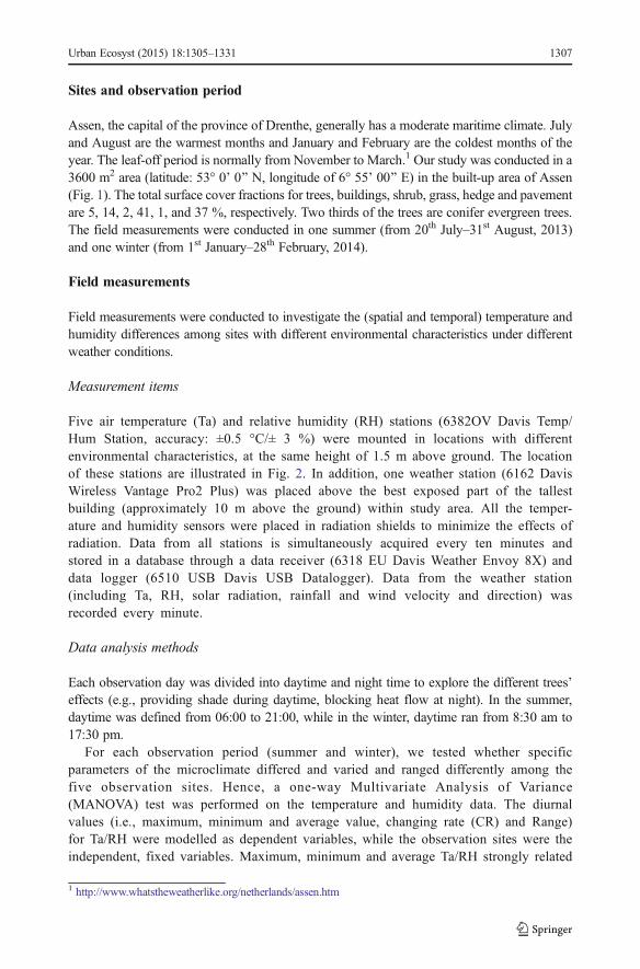
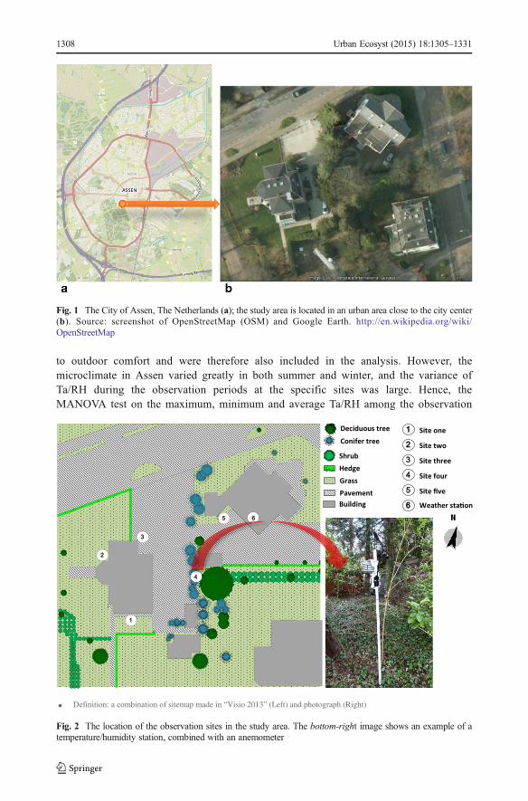
Assen, the capital of the province of Drenthe, generally has a moderate maritime climate. Julyand August are the warmest months and January and February are the coldest months of theyear. The leaf-off period is normally from November to March.1 Our study was conducted in a3600 m2 area (latitude: 53° 0’ 0^ N, longitude of 6° 55’ 00^ E) in the built-up area of Assen(Fig. 1). The total surface cover fractions for trees, buildings, shrub, grass, hedge and pavementare 5, 14, 2, 41, 1, and 37 %, respectively. Two thirds of the trees are conifer evergreen trees.The field measurements were conducted in one summer (from 20th July–31st August, 2013)and one winter (from 1st January–28th February, 2014).

Field measurements

Field measurements were conducted to investigate the (spatial and temporal) temperature andhumidity differences among sites with different environmental characteristics under differentweather conditions.

Measurement items

Five air temperature (Ta) and relative humidity (RH) stations (6382OV Davis Temp/Hum Station, accuracy: ±0.5 °C/± 3 %) were mounted in locations with differentenvironmental characteristics, at the same height of 1.5 m above ground. The locationof these stations are illustrated in Fig. 2. In addition, one weather station (6162 DavisWireless Vantage Pro2 Plus) was placed above the best exposed part of the tallestbuilding (approximately 10 m above the ground) within study area. All the temper-ature and humidity sensors were placed in radiation shields to minimize the effects ofradiation. Data from all stations is simultaneously acquired every ten minutes andstored in a database through a data receiver (6318 EU Davis Weather Envoy 8X) anddata logger (6510 USB Davis USB Datalogger). Data from the weather station(including Ta, RH, solar radiation, rainfall and wind velocity and direction) wasrecorded every minute.

Data analysis methods

Each observation day was divided into daytime and night time to explore the different trees’effects (e.g., providing shade during daytime, blocking heat flow at night). In the summer,daytime was defined from 06:00 to 21:00, while in the winter, daytime ran from 8:30 am to17:30 pm.

For each observation period (summer and winter), we tested whether specificparameters of the microclimate differed and varied and ranged differently among thefive observation sites. Hence, a one-way Multivariate Analysis of Variance(MANOVA) test was performed on the temperature and humidity data. The diurnalvalues (i.e., maximum, minimum and average value, changing rate (CR) and Range)for Ta/RH were modelled as dependent variables, while the observation sites were theindependent, fixed variables. Maximum, minimum and average Ta/RH strongly related

1 http://www.whatstheweatherlike.org/netherlands/assen.htm

Urban Ecosyst (2015) 18:1305–1331 1307

to outdoor comfort and were therefore also included in the analysis. However, themicroclimate in Assen varied greatly in both summer and winter, and the variance ofTa/RH during the observation periods at the specific sites was large. Hence, theMANOVA test on the maximum, minimum and average Ta/RH among the observation

Fig. 1 The City of Assen, The Netherlands (a); the study area is located in an urban area close to the city center(b). Source: screenshot of OpenStreetMap (OSM) and Google Earth. http://en.wikipedia.org/wiki/OpenStreetMap

Fig. 2 The location of the observation sites in the study area. The bottom-right image shows an example of atemperature/humidity station, combined with an anemometer

1308 Urban Ecosyst (2015) 18:1305–1331

sites might be obscured. We therefore calculated the differences between these factorsand their mean values for all sites D(t). A one-way MANOVA was then performed forthese differences.

D tð Þd j ¼ max.min

.averagei xd ji

� �−1

M

XM

j¼1

max.min

.averagei xd ji

� � ð1Þ

Where t stands for maximum, minimum and average Ta/RH, and x stands for Taand RH.

In addition, CR and Range are also important because they implies the level and amount ofTa/RH change along a day regardless of average temperature or seasons. The one-wayMANOVA, Tukey post-hoc tests helped to compare the different observation sites. For allour statistical analysis, significance was defined as a P value less than 0.05. The CR and Rangeare expressed as:

CRd j ¼X N

i¼1maxi xd ji

� �−xd ji

� �

N maxi xd ji� �

−mini xd ji� �� � ð2Þ

Ranged j ¼ maxi xd ji� �

−mini xd ji� � ð3Þ

Where x stands for Ta and RH, with the different parameters defined below:

j index of observation site (j=1,…, M), M=5M total number of observation sitesd index of observation day (d=1,…, K), K=43 in summer and 58 in winterK total number of observation days in summer and winteri index of data point in one day (i=1,…, N), N=144N total number of data points in one day

First, the differences of these factors were tested among all the five observationsites to prove the spatial variation in the study area. Second, we compared thesemicroclimatic factors between shaded and unshaded sites (i.e., Site one and four) bysubtracting the values from the shaded site from the unshaded site. This comparisonindicates the level of microclimate regulation by the trees. Additionally, as thebiophysical processes involved in microclimate regulation by trees are affected bythe weather conditions (c.f. Wang et al. 2014), the trees’ effect on microclimateshould be evaluated under similar weather conditions. The influence of weatherconditions on the trees’ cooling effects was detemined afterwards. All of these effectsshould be bigger than the range of measurement accuracy (i.e., ≥ 0.5 °C/3 %).

Clustering weather conditions

In order to classify the weather conditions of the observation days, we utilized a clusteringmethod, which included three features: clearness index (Kt), fluctuation of solar radiation (FR),and maximum Ta (MaxTa). After defining the cluster boundaries, t both summer and winterobservation days were clustered separately.

Urban Ecosyst (2015) 18:1305–1331 1309

Clearness index (Kt)

Kuye and Jagtap (1992) proposed a clearness index (ranging from 0 to 1) to characterize thesky conditions. Larger values represent clear weather, while low values represent cloudyweather. The index is calculated as the ratio of the global solar radiation measured at thesurface and the clear sky solar radiation:

Ktd ¼ Rd

.R0d ð4aÞ

With the global solar radiation R based on the hourly average solar insolation (measured atweather station with 1 min sample interval). The clear sky solar radiation, R0 is given by:

R0 ¼ 0:75þ 2� 10−5z� �

Ra ð4bÞThe elevation z of the weather station was 15 m above sea level (elevation of the study

height plus height of the weather station). The extraterrestrial radiation Ra for each day wasdetermined by the geographical position and the time of the year, according to:

Ra ¼ T*G*dr

πωsinφsinδ þ cosφcosδsinω½ � ð4cÞ

Where T is the length of day (24 h), G is the solar constant (1353 W/m2), dr is the inverserelative distance Earth-Sun, ω is the sunset hour angle, φ is the latitude and δ is the solardeclination.

Fluctuation of solar radiation (FR)

Since the clearness index Kt only represents the daily value based on the hourly average solarinsolation, it fails to capture the variation of solar intensity in the daily pattern. Therefore, weincluded the fluctuation rate (FR) of solar radiation to compute the variation of sunlightintensity for a given period. To determine the fluctuation rate of diurnal solar radiation (FR),we first de-trended the solar radiation time series (Rdi) by subtracting the local trend value(Rdi

fit), and then calculated the root-mean-square of the cumulative difference between mea-surements and the local trend as:

FRd ¼

ffiffiffiffiffiffiffiffiffiffiffiffiffiffiffiffiffiffiffiffiffiffiffiffiffiffiffiffiffiffiffiffiffiffiffi1

N

XN

i¼1

Rdi−Rfitdi

� �2

vuut ð5Þ

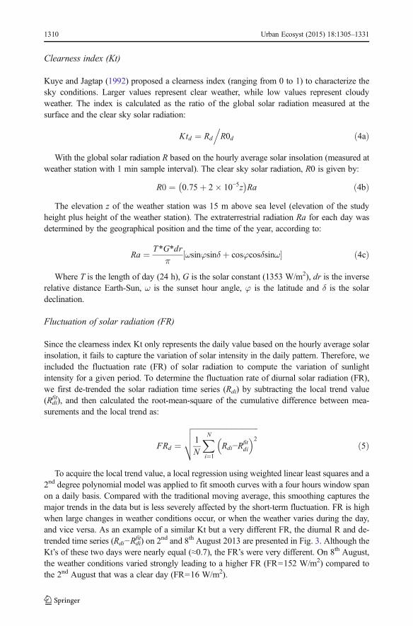
To acquire the local trend value, a local regression using weighted linear least squares and a2nd degree polynomial model was applied to fit smooth curves with a four hours window spanon a daily basis. Compared with the traditional moving average, this smoothing captures themajor trends in the data but is less severely affected by the short-term fluctuation. FR is highwhen large changes in weather conditions occur, or when the weather varies during the day,and vice versa. As an example of a similar Kt but a very different FR, the diurnal R and de-trended time series (Rdi−Rdifit) on 2nd and 8th August 2013 are presented in Fig. 3. Although theKt’s of these two days were nearly equal (≈0.7), the FR’s were very different. On 8th August,the weather conditions varied strongly leading to a higher FR (FR=152 W/m2) compared tothe 2nd August that was a clear day (FR=16 W/m2).

1310 Urban Ecosyst (2015) 18:1305–1331

Maximum Ta (MaxTa)

To investigate the effects of trees on extremely uncomfortable days, the maximum airtemperature during the day (MaxTa) is also included as a feature for the clustering of theweather conditions. It highlights the hot days and relates to outdoor comfort level.

Definition of clusters

To define the clusters, FR and MaxTa were normalized to switch to the same scale as Kt,using:

F fð Þd ¼f d−mind f dð Þ

maxd f dð Þ−mind f dð Þ ð6Þ

In this formula f stands for FR and MaxTa. The terms max(f) and min(f) are the maximumand minimum values among the observation days in the summer and winter respectively. Weadopted a fast clustering method to classify the synoptic weather conditions using fixed clusterboundaries for all features. A value of 0.5 was set as cluster boundary for all the tree featuresincluded in this analysis. After the permutation and combination of the Kt, F(FR) andF(MaxTa), the observation days were classified into eight clusters. Note that the normalizationprocess leads to cluster boundaries that depend on the dataset itself. Hence, if the changes ofthe weather conditions were negligibly small during the observation days, this clusteringmethod may fail. Since the observation days should cover a variety of different weatherconditions, a long-term observation period is essential for this method.

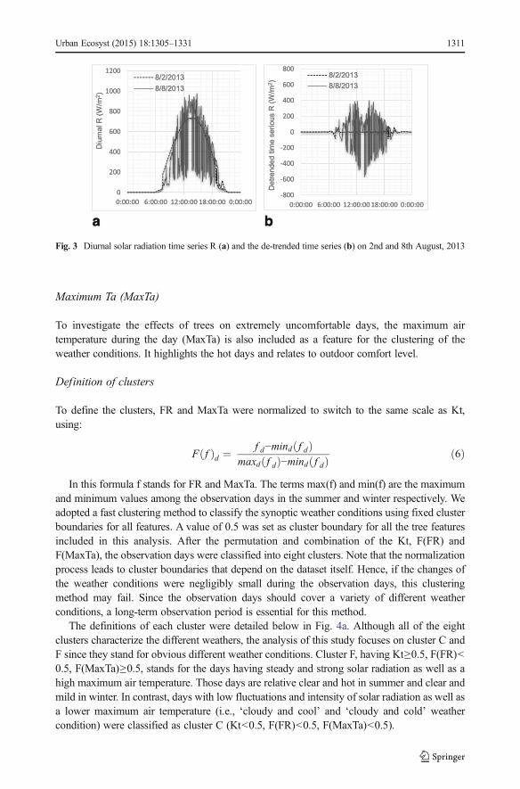
The definitions of each cluster were detailed below in Fig. 4a. Although all of the eightclusters characterize the different weathers, the analysis of this study focuses on cluster C andF since they stand for obvious different weather conditions. Cluster F, having Kt≥0.5, F(FR)<0.5, F(MaxTa)≥0.5, stands for the days having steady and strong solar radiation as well as ahigh maximum air temperature. Those days are relative clear and hot in summer and clear andmild in winter. In contrast, days with low fluctuations and intensity of solar radiation as well asa lower maximum air temperature (i.e., ‘cloudy and cool’ and ‘cloudy and cold’ weathercondition) were classified as cluster C (Kt<0.5, F(FR)<0.5, F(MaxTa)<0.5).

a b

-800

-600

-400

-200

0

200

400

600

800

0:00:00 6:00:00 12:00:00 18:00:00 0:00:00

Det

rend

ed ti

me

serio

us R

(W/m

2 )

8/2/20138/8/2013

0

200

400

600

800

1000

1200

0:00:00 6:00:00 12:00:00 18:00:00 0:00:00

Diu

rnal

R (W

/m2 )

8/2/20138/8/2013

a b

-800

-600

-400

-200

0

200

400

600

800

0:00:00 6:00:00 12:00:00 18:00:00 0:00:00

Det

rend

ed ti

me

serio

us R

(W/m

2 )

8/2/20138/8/2013

0

200

400

600

800

1000

1200

0:00:00 6:00:00 12:00:00 18:00:00 0:00:00

Diu

rnal

R (W

/m2 )

8/2/20138/8/2013

Fig. 3 Diurnal solar radiation time series R (a) and the de-trended time series (b) on 2nd and 8th August, 2013

Urban Ecosyst (2015) 18:1305–1331 1311

Clustering results

Figure 4b represents the clustering results for both summer and winter observation days. In thesummer, 43 observation days fell under six clusters (A-F). Most of these days (40 %) wererelatively cloudy and cool (cluster C), whereas only 7 days (16 %) were relatively clear and hot(cluster F). Among the 58 observation days in the winter, most days (80 %) were cloudy(cluster C and G), indicated by a low Kt (<0.5) and F(FR) (<0.5). However, only 11 days(19 %) had a low F(MaxTa) (<0.5) and fell under cluster C. Additionally, clear and mildweather conditions (cluster F) were found in 6 days (10 %).

The features mentioned in Section 2.2.2 were computed and compared among differentclusters. Furthermore, representative days were selected from the ‘cloudy and cool’ and ‘cloudyand cold’ clusters C and ‘clear and hot’ and ‘clear andmild’ clusters F for the model simulation.

Numerical modelling

Three-dimensional numerical microclimate simulations using ENVI-met were conducted toexplore the relation between tree characteristics and temperature and humidity distribution inthe study area. Based on the fundamental laws of fluid dynamics and thermodynamics, ENVI-met is designed to simulate surface-plant-air interactions in an urban environment (Bruse2010) and has been used in different studies (Emmanuel et al. 2007; Fahmy et al. 2009;Hedquist and Brazel 2014; Middel et al. 2014). ENVI-met allows to simulate the urbanenvironment from a microclimate scale to the local climate scale with a resolution of 0.5 to10 m in space and 10 s in time with 250 grids at maximum. In this study, the geometry,buildings, vegetation, and surface materials of the study area are defined on a 3D grid of 120×120×30 cells, with a 0.5 m grid cell size. This resolution allows to investigate local microcli-mate variations (Bruse 2010). The geometry, plant and soil database, and building propertiesspecified for this study were based on data from the Top10NL map2 and measurements. For

2 https://www.kadaster.nl/web/artikel/productartikel/TOP10NL.htm

Clusters Kt F(FR) F(MaxTa)

A ≥ 0.5 ≥ 0.5 < 0.5;

B ≥ 0.5 < 0.5 < 0.5;

C < 0.5 < 0.5 < 0.5;

D < 0.5 ≥ 0.5 < 0.5;

E ≥ 0.5 ≥ 0.5 ≥ 0.5;

F ≥ 0.5 < 0.5 ≥ 0.5;

G < 0.5 < 0.5 ≥ 0.5;

H < 0.5 ≥ 0.5 ≥ 0.5;

a b

28

17

81

70 0

0

5

10

15

20

A B C D E F G H

NO

. DA

YS

43 observation days in summer

0 0 11 0 4 6

35

20

10

20

30

40

A B C D E F G H

NO

. DA

YS

58 observation days in winter

Fig. 4 The definitions of clusters of the synoptic weather conditions (a) and clustering results for the summerand winter observation days (b)

1312 Urban Ecosyst (2015) 18:1305–1331

the plant database, ENVI-met requires the vertical distribution of leaf area density in tendifferent heights. We first determined the vegetation leaf index (LAI) of the trees within modelarea with a LAI-2000 Plant Canopy Analyser under cloudy weather condition. Subsequently,leaf area density values in ten different heights were calculated using the method by Lalic andMihailovic (2004). In addition, the field measurements were used as the input data for modelinitialization. These include wind velocity, wind direction, initial air temperature, relative andspecific humidity, and indoor temperature.

In addition, ENVI-met allows to select the points inside the model area where the processesin the atmosphere and the soil are calculated in more detail. These selected points are named‘receptors’. In order to capture this detailed information within the study area, 81 equidistantreceptors were added in the area input file (labelled AA–II in Fig. 5). However, the 13receptors that were located on the façade of buildings, did not monitor the outdoor processesand were eliminated from the statistical analysis. After running a 24 h simulation with a halfhour interval the following features were extracted from the receptors at 1.5 m height: Ta andRH, wind velocity (Va), longwave and shortwave radiation, and the Predicted Mean Vote(PMV). The PMV methodology determines thermal comfort (ISO 7726 1998), ranging from -3=‘very cold’ to +3=‘very hot’) (Matzarakis and Mayer 1998); and is calculated by combin-ing Ta, RH and Va with parameters that describe the heat exchange processes of the humanbody. To calculate PMV in ENVI-met, we set biometeorological values for people’s slow walkto 1.4 m/s and a 150 W/m2 energy exchange. Thermal resistance of clothing was adjusteddepending on summer and winter clothing.

Fig. 5 ENVI-met map of the study area where 81 equidistant receptors are indicated with a grid identifierranging from AA to II. The blue circles represent 13 receptors located on the façade of buildings; while the redcircles indicate the rest receptors

Urban Ecosyst (2015) 18:1305–1331 1313

Selection of comparable days and model validation

Using the clustering results, four days in the summer and winter were selected at random fromcluster C and F (i.e., 2nd, 3rd August, 2013 and 18th, 21st January, 2014). The weatherconditions of these selected days are shown in Table 1. On the clear days (e.g., 2nd Augustand 18th January), the daily total solar radiation was much higher than on cloudy days. Thewind velocity was less than 3 Beaufort (<11 km/h) during these four days. The dominant winddirection was SE on both ‘clear and hot’ summer day and ‘clear and mild’ winter day, but SWon the ‘cloudy and cool’ summer day and ‘cloudy and cold’ winter day.

An evaluation of the accuracy of predicted ENVI-met (P) values with observed temperatureat five sites was performed among these four selected days. Figure 6 shows the results fromSites one and four on August 2nd as an example. A notable contrast between the observed andsimulated Ta can be observed. As expected, the maximum Ta within the tree canopy (Site four)was approximately 1 °C lower than that of the area without trees. However, the simulation andmeasurement results show two discrepancies. First, the simulation results tend to underesti-mate daytime temperatures and overestimate night-time temperatures. Second, the poorermodel performance appeared in the afternoon when temperature and humidity strongly swung.ENVI-met failed to simulate these rapid microclimatic changes. One of ENVI-met’s limita-tions is that its simulation output is time and space (within one grid) averaged (Emmanuel et al.2007; Peng and Jim 2013). Therefore, the diurnal temperature variations are contracted.Furthermore, the simulated data cannot represent instant temperature conditions because suchmodels always keep a constant tendency (Peng and Jim 2013). The possible immediatedisturbances, which are observed from measurements, cannot be realistically reflected in themodel outputs. This leads to the underestimation of the reduction of the temperature and itsfluctuations caused by trees.

Despite this deficiency, the simulated Ta showed good qualitative agreement with themeasurements based on both correlation coefficient (R2) and error indices (root mean squareerror-RMSE and mean absolute error-MAE). Lower RMSE and MAE values indicate a bettermodel performance. The index of agreement (d), which was developed by Willmott (1981),measures the degree of model prediction error and ranges from 0 to 1. A higher value indicatesa better agreement between simulation and measurement. R2 among the five sites rangedbetween 0.73 and 0.97 on the selected two summer days, and between 0.79 and 0.95 on theselected two winter days. RMSE and MAE were low throughout all sites and d was generally>0.60. Table 2 shows the evaluation results for each site in detail on the four selected days.

Table 1 Weather conditions of selected days

Days Cluster Weathercondition

Daily total solarradiation (W/m2)

Relativehumidity (%)

Wind velocity(km/h)

Dominant winddirection

Summer

2nd, Aug, 2013 F Clear 6378.82 69 % 6.8 SSE

3rd, Aug, 2013 C Cloudy 4906.10 71 % 10.7 WSW

Winter

18th, Jan, 2014 F Clear 614.03 92 % 5.1 ESE

21st, Jan, 2014 C Cloudy 101.73 96 % 3.2 WSW

1314 Urban Ecosyst (2015) 18:1305–1331

a b

15

20

25

30

35

40

0 2 4 6 8 10 12 14 16 18 20 22 24

Ta (°

C )

Hours

Site ONE (unshaded)

Observed

Simulated

15

20

25

30

35

40

0 2 4 6 8 10 12 14 16 18 20 22 24

Ta (°

C )

Hours

Site FOUR (shaded)

ObservedSimulated

Fig. 6 Measured and simulated temperature values at an unshaded site (a) and shaded site (b) on the 2nd August,2013

Table 2 R2, RMSE, RSR, MAE and d between the measured and the computed air temperatures in 24 h period

Days Correlationcoefficient R2

Root mean squareerror RMSE (°C)

Mean absoluteerror MAE (°C)

Index ofagreement d

Summer

2nd, Aug, 2013

Site one 0.97 0.66 0.41 0.97

Site two 0.96 0.14 0.89 0.99

Site three 0.95 0.65 0.35 0.98

Site four 0.98 0.90 0.76 0.96

Site five 0.95 0.76 0.56 0.97

21st, Jan, 2014

Site one 0.92 1.47 1.13 0.73

Site two 0.81 1.66 1.18 0.70

Site three 0.82 2.13 1.71 0.73

Site four 0.81 1.65 1.41 0.68

Site five 0.73 1.97 1.62 0.63

Winter

18th, Jan, 2014

Site one 0.89 0.70 0.60 0.87

Site two 0.91 0.86 0.79 0.80

Site three 0.91 0.63 0.45 0.89

Site four 0.91 0.61 0.42 0.88

Site five 0.95 0.64 0.43 0.87

21st, Jan, 2014

Site one 0.81 0.28 0.25 0.85

Site two 0.79 0.28 0.24 0.85

Site three 0.87 0.64 0.63 0.64

Site four 0.86 0.54 0.51 0.70

Site five 0.85 0.31 0.27 0.81

Urban Ecosyst (2015) 18:1305–1331 1315

Simulation design and data analysis

In order to examine the effects of the trees at the study site on the microclimate and thermalcomfort, we compared the simulations of the current situation (CU) (i.e., with 5 % total treecover and 3 % evergreen tree cover in the summer and winter, respectively) and no tree (NT)conditions on selected days. In the NT simulation, we removed all the trees, including bothdeciduous and evergreen trees, from the model area.

First, we investigated how trees affect the microclimate over the entire area. Based on the24 h simulations for all 68 receptors, the maximum, minimum and average CR and Range forair temperature were calculated. The mean of these features for all the receptors was derivedseparately on the four selected days as expressed in Eq. 7.

Mean of receptors ¼ 1

M

XM

j¼1

DFcuj−DFnt j� � ð7Þ

In this formula, M is the number of the receptors and j is the index of receptors. DFcu andDFnt are the daily values of different features in the CU and NT simulations, respectively. Wecalculated the difference between DFcu and DFnt, and then derived the average value for allthe receptors.

Second, we investigated if the spatial temperature distribution changes over time. The Tadifferences (ΔTaji) between CU and NTsimulations were calculated at each receptor j and eachtime step i. To quantify the spatial differences of the effects of the trees, the time-series range ofΔTa among the receptors is defined in Eq. 8.

Range of ΔTað Þi ¼ maxj ΔTaji

� �−minj ΔTaji

� � ð8ÞWhere the terms of maxj(ΔTaji) and minj(ΔTaji) are the maximum and minimum Ta of 68

receptors at time i. Time and place in which the temperature was greatly influenced by the treesis determined in this way.

Due to the effects on the microclimate, trees altered the outdoor human comfort level as well,especially during the hottest hours of the day (from 12:00 to 18:00). After extracting the PMVvalue during the hottest hours from ENVI-met, we calculated the occurrence frequency of thePMV value at different scales under CU and NT conditions. The comparison between CU andNT conditions helped us to analyse how the trees determine the outdoor human comfort.

Results

Measurement results

Effect of trees on microclimate in the summer

Microclimatic differences among the observation sites During daytime in the summerperiod, a significant difference in CR and Range of Ta/RH among the observations sites wasrevealed by one-way MANOVA (p<.0005). In terms of the air temperature, the observationlocation has a statistically significant effect on both CR (p=.033 ) and Range (p<.0005). Theresults from the multiple comparisons showed that CR and Range of Site one were significantly

1316 Urban Ecosyst (2015) 18:1305–1331

different from that of the other sites (p<.05 for both CR and Range). Similar results were alsofound for RH. Generally speaking, the variation rates and ranges of air temperature andhumidity varied significantly among the observation sites. Although the maximum, minimumand average Ta/RH did not show significant differences for the observation sites, the differencesbetween these features and their mean values of all sites, i.e., D(t), were significant (p<.0005 forall). Hence, we conclude that, during the daytime of the summer period, the microclimaticconditions at the observation sites had significant differences. In terms of the microclimate atnight, the spatial differences of temperature and humidity were significant among the sites, withD(t) of Ta/RH varied significantly among the different sites (p<.0005 for all).).

Microclimatic differences between shaded and unshaded areas According to thestatistical tests, tree canopy significantly reduced CR by approximately 0.04 (standard devi-ation (SD)=0.03) and the Range of Ta by 2.4 °C (SD=0.9 °C) in the daytime. This means thattrees efficiently reduce the daily temperature difference and variation during the hot months.Moreover, the shade of trees reduced the air temperature significantly during daytime with D(t)(p<.05 for all). Fig. 7 illustrates the differences in average and maximum Ta between theshaded and unshaded area during this period. This difference was computed by subtracting Tameasured in shaded areas from that of unshaded areas. The average Ta and RH in tree coveredareas was 1 °C (SD=0.4 °C) lower and 3 % (SD=1.2 %) higher than those of unshaded areas.However, the differences of maximum Ta and minimum RH were enlarged to 2.5 °C (SD=0.9 °C) and 5 % (SD=2.3 %), while they could reach a maximum of 4.1 °C and 10 % at noon.At night, the tree covered area has a slightly lower Range of Ta (approximately 0.1 °C). Thisdifference was also observed on the calm or light air days with relatively little heat convection.

Weather effects in the daytime To investigate the weather effects on the microclimaticcondition, the comparison of Ta and RH between relatively cloudy and cool days (cluster C)and clear and hot days (cluster F) during the daytime was made, highlighted by respectivelycircles and triangles in Fig. 7. The results revealed that on the cloudy and cool days, both CRand the Range of Ta/RH was not significantly different among the sites (p>.05 for all).However, these features differ significantly for the different sites on the clear and hot days(p<.0005 for all). In addition, the differences of D(t) for Ta/RH among the different sites weresignificant on both cloudy and cool days and clear and hot days, with p<.0005 for all the

0

1

2

3

4

5

Ave

rage

Ta

(°C

)

Ta unshaded - Ta shaded(°C)

Difference of Average Ta Clear and hot daysDifference of Max Ta Cloudy and cool days

0

1

2

3

4

5

7/20/2013 7/27/2013 8/3/2013 8/10/2013 8/17/2013 8/24/2013 8/31/2013

Max

Ta

(°C

)

Fig. 7 Difference in average and maximum Ta between the shaded and unshaded site of the trees in the summerdaytime (from 06:00 to 21:00)

Urban Ecosyst (2015) 18:1305–1331 1317

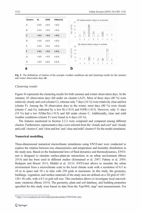
features. Figure 8 shows the maximum, minimum and average Ta and RH for each observationsite, on average during both cloudy and cool and clear and hot days.

We compared the maximum,minimum and average Ta and RH in the shaded area with thoseones in the unshaded area. On relatively cloudy and cool days, the maximum and average Tawithin the tree canopy were approximately 1.8 °C (SD=0.7 °C) and 0.8 °C (SD=0.2 °C) lowerthan those of the unshaded area. These temperature differences were enlarged to 3.2 °C (SD=0.5 °C) and 1.5 °C (SD=0.2 °C) on relatively clear days. The average RH of shaded areasexceeds that of unshaded areas by 3 % (SD=0.8 %) on cluster C days, and 3 % (SD=1.4 %) oncluster F days. In general, on relatively clear and hot days, the Ta reduction by the trees wasabout two times higher than that on the cloudy and cold days. A table summarizing daytime Taand RH between cloudy and cool and clear and hot days is shown in Appendix 1.

Fig. 8 Comparison of maximum, minimum and average Ta (a) and RH (b) at five sites between cloudy and cooland clear and hot days

0

0.5

1

1.5

Ave

rage

Ta

(°C

)

Ta unshaded - Ta shaded (°C)

Difference of Average Ta Clear and mild daysDifference of Max Ta Cloudy and cold days

0

0.5

1

1.5

1/1/2014 1/8/2014 1/15/2014 1/22/2014 1/29/2014 2/5/2014 2/12/2014 2/19/2014 2/26/2014

Max

Ta

(°C

)

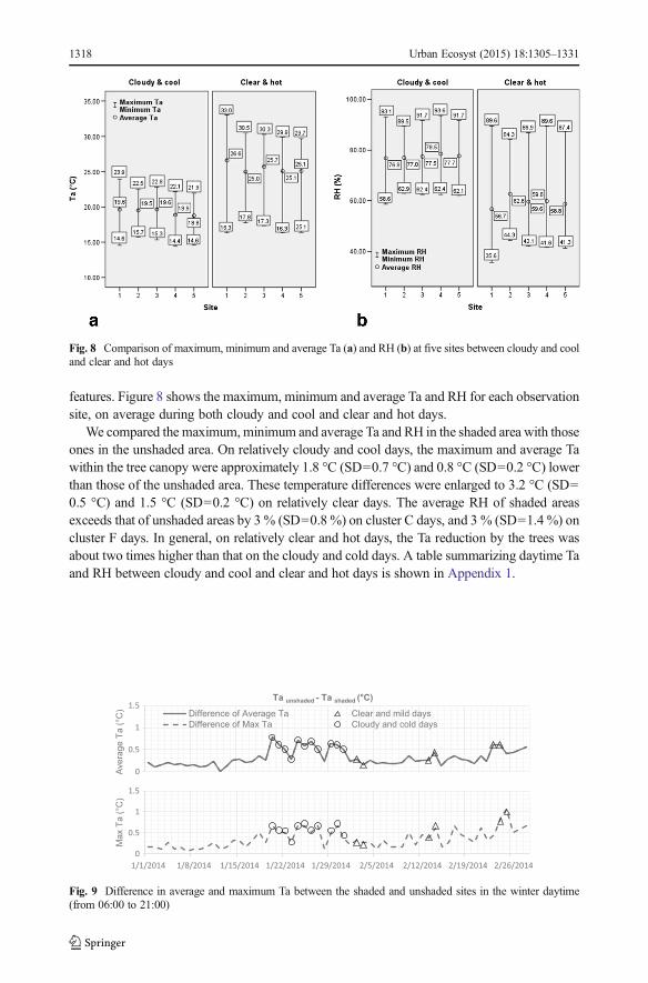
Fig. 9 Difference in average and maximum Ta between the shaded and unshaded sites in the winter daytime(from 06:00 to 21:00)

1318 Urban Ecosyst (2015) 18:1305–1331

Effect of trees on microclimate in the winter

Microclimatic differences among the observation sites Although the effects of trees didnot lead to significant differences in CR and Range for Ta/ RH (p>.05 for all) during bothdaytime and night time, the distribution of air temperature and humidity was significantly

-0.5

0

0.5

1

1.5

2

0:00:00 6:00:00 12:00:00 18:00:00 0:00:00

∆Ta

(°C

)

2nd August, 201381 receptors Average

Ta NT - Ta CU

-0.5

0

0.5

1

1.5

2

0:00:00 6:00:00 12:00:00 18:00:00 0:00:00

∆Ta

(°C

)

3rd August, 2013

-0.5

0

0.5

1

1.5

2

0:00:00 6:00:00 12:00:00 18:00:00 0:00:00

∆Ta

(°C

)

18th January, 2014

-0.5

0

0.5

1

1.5

2

0:00:00 6:00:00 12:00:00 18:00:00 0:00:00

∆Ta

(°C

)

21st January, 2014

Fig. 10 The differences of ΔTa under CU and NT conditions among 68 receptors on selected days

2%11%

4% 9%

74%

1%6% 2% 1%

90%

0%

20%

40%

60%

80%

100%

1.5 - 2.5 2.5 - 3.5 3.5 - 4.5 4.5 - 5.5 > 5.5

Current condition No tree

(Warm) (Hot) (Very hot)

3%

44%54%

2%

33%

65%

0%

20%

40%

60%

80%

100%

0.5 - 1.5 1.5 - 2.5 2.5 - 3.5(Slightly warm) (Warm) (Hot)

Fig. 11 Frequency of PMV value at different scales from 12:00 to 18:00 on clear and hot day (a) and cloudy andcool day (b)

Urban Ecosyst (2015) 18:1305–1331 1319

different (p<.0005 for all the D(t) of Ta/RH in both daytime and night time) among theobservation sites.

Microclimatic differences between shaded and unshaded area The positive coolingeffect of 3 % by evergreen trees in the study area in the summer may lead to disservices in thewinter. In the daytime there was no significant difference in CR and Range of Ta/RH betweenshaded and unshaded area but we found that the trees significantly lowered the average Ta andraised the average RH by respectively 0.5 °C (SD=0.2 °C) and 3 % (SD=0.6 %). Themaximum differences of maximum Ta and minimum RH were up to 1 °C and 5 % at noon(Fig. 9). The decreased air temperature may lead to an increase of heating energy consumptionand a decline of outdoor thermal comfort.

Theoretically, at night, tree canopy prevents the heat flow from the surface to the surround-ings and slows down heat losses, thus increasing the Ta and lowering the CR and Range of Ta.However, the measured effect of the evergreen trees on the microclimate at night was notsignificant, with p>.05 for both the trends and values of Ta. Wind velocity was a significantfactor in explaining the Ta range differences between the shaded and unshaded area, with p=0.042. On calm or light air days, the Ta range was slightly lowered by the trees.

Weather effects in the daytime In terms of the weather effects during the daytime in winter,the statistical tests indicated that no significant differences on either measured value or trend forboth Ta and RH between cloudy and cold and clear and mild days (p>.05 for all) were found(see also the marked days by the circles and triangles in Fig. 9). Accordingly, we concluded thatthe weather conditions in the winter did not cause a notable change on performance of trees onthe microclimate. Appendix 2 summarizes the daytime maximum, minimum and average Taand RH under the cloudy and cold and clear and mild weather conditions.

Modelling results

Effect of trees on outdoor microclimate

Appendix 3 shows the maximum, minimum and average air temperature for both current (CU)and no-tree (NT) conditions on selected days in detail. To better understand the impact of thetrees on the microclimatic condition, we calculated the Ta difference (ΔTa) caused by theabsence of trees (i.e., Ta in CU condition was subtracted from Ta in NT condition at eachreceptor and each time step for four selected days). Fig. 10 represents the ΔTa between CU andNT for all the receptors in 24 h.

Spatial variation on the summer days On a selected clear and hot day (2nd August 2013),5 % tree cover reduced maximum Ta with 1.1 °C (SD=0.23 °C). At Site four with trees, themaximum Ta differed by as much as 1.4 °C for simulated situations with and without trees. Inaddition, trees reduced the daily Range of Ta by approximately 1 °C (SD=0.24 °C). Unlike theremarkable differences in the Range, the differences of CR between CU and NT conditionswere small. Appendix 4 shows the daily average value, CR and Range for Ta in both CU andNT conditions on a clear and hot day. On the selected cloudy and cool day (3rd August 2013),the influence of trees on Ta was much smaller, with only 0.3 °C (SD=0.05 °C) maximum Tareduction at Site four. The reduction of CR and Range was small.

1320 Urban Ecosyst (2015) 18:1305–1331

Although the simulated results cannot reflect the large fluctuation in air temperature andhumidity at a specific location (see 3.2.1), the differences in the effect of trees among thereceptors were notable. On the clear and hot day, the range of ΔTa between the area with thestrongest effect and the area with the weakest effect was about 0.6 °C (SD=0.41 °C) onaverage. This range went up to 1.5 °C at the time of the peak reduction at 18:00 (Fig. 10). Thespatial variation on the cloudy and cool day was much smaller than that on the clear and hotday. The daily average range of ΔTa was about 0.2 °C (SD=0.03 °C), and went up to 0.3 °C at13:30.

Spatial variation on the winter days According to the simulation results, the reductions ofmaximum Ta were estimated to be 0.2 °C (SD=0.05 °C) and less than 0.1 °C (SD=0.02 °C),on the clear and mild day and the cloudy and cold day (i.e., 18th and 21st January 2014),respectively. During the afternoon of these two winter days, the temperature in areas with treeswas slightly higher than in area without trees. This was reflected by the negative values of ΔTain Fig. 10, which could increase human thermal comfort. The effect of these trees on the CRand Range of Ta was negligiblely small.

Among the receptors from the locations far from to close to the trees, the daily averagerange of ΔTa was about 0.2 °C (SD=0.14 °C) on clear and mild days. The variation of ΔTaamong the receptors reached a peak at 15:30, with 0.5 °C difference between the areas with thestrongest and weakest effect (Fig. 10). On the cloudy and cold winter day, the effect of trees onthe temperature distribution was small. Hence, the spatial differences of ΔTa tended to be smallas well (i.e., less than 0.1 °C on average).

Effect of trees on outdoor thermal comfort

Predicted mean vote on the summer days To better understand how trees affect outdoorthermal comfort during the hottest hours in the summer, the PMV value during 12:00–18:00 ateach receptor was derived from the model results under CU and NT conditions respectively.Figure 11 shows the occurrence frequency of the PMV value at different scales from 12:00 to18:00 on both clear and hot days and cloudy and cool days.

On the clear and hot day, tree shading during the hottest hours significantly influenced humancomfort simulation results. Comparison of the average PMV indicates that in this period treescould reduce the high PMVof>5.5 °C by 16 % while increasing the low PMVof 1.5–2.5 °C by1% and 2.5–3.5 °C by 5%. Although the comfort level in most areas was still uncomfortable it isbetter than the ‘very hot’ thermal perception experienced for the same time period at all otherplaces within model area. Under the tree canopy, the PMV value was decreased by 2.7 °C. Duringthe hottest hours of the cloudy and cool day, the ‘hot’ thermal perception (2.5–3.5 °C) wasreduced by 11 %. The moderation of temperature at night by trees led to different effects onhuman comfort depending on the weather conditions. However, these impacts were small withthermal perceptions ranging from ‘comfortable’ to ‘warm’. Appendix 5 and Appendix 6 displaythe comfort level under CU and NT condition at 14:00 and 22:00 of the selected days.

PMV value on the winter days During the two selected days in the winter, the comfort washighest in the afternoon hours. On the clear and mild day, PMV values, though slightly lowerin the shade, were estimated to be at ‘comfort’ and ‘slightly warm’ levels over the entire area(Appendix 5). In theory, evergreen trees could improve human comfort at night by retarding

Urban Ecosyst (2015) 18:1305–1331 1321

heat losses and reducing the cold wind blowing and block the heat loss. However, the changeson the comfort level were negligible small on both selected days (Appendix 6).

Discussion

Measurement results

Microclimatic differences

The measurement results confirmed that tree covered areas show lower average airtemperature during the daytime in the summer than the unshaded area by approximately1 °C. This agrees with previous studies that reported a 0.9–2 °C reduction of averageambient air temperature in areas with vegetative canopy (McPherson et al. 1989; Tahaet al. 1991; Park et al. 2012). Additionally, previous studies proved that evergreen treesalso reduce the temperature in the winter (Akbari 2002; Mcpherson 1988). This was alsoobserved in our measurements.

Theoretically, evergreen trees can prevent the vertical heat transfer and reduce the heatexchange between areas below and above the canopy at night in the winter (Akbari 2002;Heisler and Grant 2000; Mcpherson 1988), thereby increasing the Ta and lowering the CR andRange of Ta. However, this has not been observed from our measurements. A plausibleexplaination is that the heat convection in the winter was strong. This affected the temperaturespatial distributation, since the wind velocity was a significant factor in explaining thedifferences of Range of Ta between the shaded and unshaded area.

Weather effects

In our study we used a cluster methodology to characterise the sky conditions, integrat-ing the clearness index, the variation of solar intensity and the maximum air temperature.Cooling effects of trees on relatively clear and hot days were about two times higher thanon the cloudy and cold days. Similar results were also reported by another study thatinvestigated the thermal conditions of the typical shaded and un-shaded buildings in thesummer and dry season (December–February) in Nigeria (Morakinyo et al. 2013). Theyanalyzed the variation of outdoor air temperature in relation to different weather condi-tions. A clearness index was used to characterize weather conditions. Their resultsconfirmed that the influence of trees on the outdoor air temperature became less withthe increase of cloudiness.

Our findings also indicate that, during the daytime in the winter, different weather condi-tions did not cause a notable change of tree effects on microclimate. That is most likely due tothe fact that the variation of incoming solar radiation under the different weather conditionswas rather small because of the low solar intensity.

Modelling results

Numerical models such as ENVI-met probably introduce a bias in the simulations. The modelresults poorly represent instant temperatures and fail to capture the real instantaneous changesof air temperature and humidity. This inability of ENVI-met has been reported by several

1322 Urban Ecosyst (2015) 18:1305–1331

studies (e.g., Emmanuel et al. 2007; Peng and Jim 2013). The good simulations’ agreementwith the measurements, however, indicated that our input parameters were adequate for thelocal scale simulations.

Spatial variation

In the summer, the spatial differences of ΔTa among the receptors in the model were found tovary strongly, being 1.5 °C and 0.2 °C at maximum values on clear and cloudy daysrespectively. In the winter, the maximum spatial differences were smaller but still apparentwith 0.5 °C and 0.1 °C on clear and cloudy days. This demonstrates that, when the weather isclear and hot, trees efficiently alter the local microclimate and cause large variations in closegeographical proximity. To better understand the effects of trees on the local urban microcli-mate and to identify and quantify the effect of urban trees on local outdoor microclimate andhuman thermal comfort, essential empirical information on the microclimate must be collectedin close geographical proximity.

Thermal comfort

We extracted the simulated PMV value from ENVI-met to illustrate the thermal perception inthe study area. The maximum PMV (i.e., extra uncomfortable thermal perception) was notablyreduced during the hottest hours on both clear and cloudy days. Fahmy et al. (2009) stated thatPMV differs depending on density of the trees. Further study in this direction is necessary tocompare the cooling effects among the trees with different density and height. Although PMVwas developed based on a huge database, human comfort levels highly depends on the humanthermal perception, expectation and preference in the particular study context (area and time).Hence, field surveys are necessary to investigate the subjective responses for people thermalsensations in the local area.

Conclusion

This study provides new insight into the role of trees on microclimate and human thermalcomfort in a local urban area through field measurements and modelling. The effect of weatherconditions on the cooling performance of trees was analysed. Observed weather conditionswere clustered to investigate the differences in cooling effect of trees and to select theappropriate days for the simulations.

The results from both the measurements and the simulations showed that trees significantlyaltered the surrounding summer microclimate. The comparison on the measurements betweenthe shaded and unshaded area showed that the daily maximum air temperature differed by2.5 °C. Significant spatial variations were caused by the trees. Trees considerably improved thethermal comfort level through reducing the ‘very hot’ and ‘hot’ thermal conditions in the studyarea. Additionally, we found that the evergreen trees also lowered the average winter airtemperature by 0.5 °C. The benefit of this effect, can potentially be offset through increasedenergy costs.

The biophysical processes involved in microclimate regulation by trees are affected by,among others, the surrounding temperature, humidity and solar radiation, whereby the coolingeffect of trees was greatly influenced by prevailing weather conditions. The measurements in

Urban Ecosyst (2015) 18:1305–1331 1323

the shaded and unshaded areas revealed that, on relatively clear and hot days, the Tareduction by the trees was about two times higher than that on cloudy and cold days.Also the simulations with ENVI-met showed strongly varying temperature conditionsspatially. Hence, when studying the influence of trees on the microclimate, weatherconditions must be considered, especially in the summer. We conclude that trees, asan important element in urban green infrastructure, are very effective in regulating themicroclimate and enhancing thermal comfort locally. Weather conditions, however,strongly influence the trees’ performance in such microclimate regulation, especiallyin the summer.

Funding This study was funded by INCAS3.

Conflict of interest The authors declare that they have no conflict of interest.

Appendix 1 Summarize table on daytime Ta and RH between cloudyand cool and clear and hot days in the daytime of summer

Weather No. of days Features Features on daily basisa Mean differences

Site one(no trees)

Site four(beneath trees)

(Site one-Site four)

Value Std.Deviation

Cloudy and cool 17 Max Ta (°C) 18.9–28.0 18.3–25.5 1.8 0.7

17 Min Ta (°C) 9.7–20.1 9.7–19.9 0.1 0.2

17 Ave. Ta (°C) 16.0–22.9 15.5–21.9 0.8 0.2

17 Max. RH (%) 79–97 79–98 −1 0.8

17 Min. RH (%) 43–83 48–84 −4 2.4

17 Ave. RH (%) 62–92 64–94 −3 0.8

Cloudy and hot 7 Max Ta (°C) 28.3–36.8 25.2–33.7 3.2 0.5

7 Min Ta (°C) 13.3–19.0 13.4–18.7 0.0 0.3

7 Ave. Ta (°C) 22.6–29.3 21.3–27.8 1.5 0.2

7 Max. RH (%) 81–96 82–98 0 1.4

7 Min. RH (%) 28–50 33–57 −6 1.3

7 Ave. RH (%) 49–70 51–75 −3 1.4

Total 43 Max Ta (°C) 18.9–36.8 17.9–33.7 2.4 0.9

43 Min Ta (°C) 9.7–20.1 9.7–19.9 0.1 0.2

43 Ave. Ta (°C) 16.0–29.3 15.2–27.8 1.0 0.4

43 Max RH (%) 79–97 79–98 0.0 1.2

43 Min RH (%) 28–83 33–84 −5 2.3

43 Ave. RH (%) 49–92 51–94 −3 1.2

1324 Urban Ecosyst (2015) 18:1305–1331

a1K ∑

K

d¼1Features on daily basisð Þ

Where: d is the index of observation day (d=1,…, K), K=17 for cloudy and cool days and7 for clear and hot days

Appendix 2 Summarize table on daytime Ta and RH between cloudyand cold and clear and mild days in the daytime of winter

a1K ∑

K

d¼1Features on daily basisð Þ

Where: d is the index of observation day (d=1,…, K), K=11 for cloudy and cool days and6 for clear and hot days

Weather No. of days Features Features on daily basisa Mean differences

Site one(no trees)

Site four(beneath trees)

(Site one-Site four)

Value Std.Deviation

Cloudy and cold 11 Max Ta (°C) −2.2–4.6 −2.7–3.9 0.6 0.1

11 Min Ta (°C) −4.2–2.0 −4.9–1.6 0.5 0.2

11 Ave. Ta (°C) −3.2–3.3 −3.9–2.8 0.6 0.1

11 Max. RH (%) 89–96 90–98 −1.8 0.4

11 Min. RH (%) 79–94 81–96 −2.2 0.6

11 Ave. RH (%) 83–95 85–97 −2.0 0.4

Clear and mild 6 Max Ta (°C) 7.6–13.4 7.4–12.7 0.5 0.2

6 Min Ta (°C) 0.2–4.4 0.4–4.3 0.1 0.2

6 Ave. Ta (°C) 5.1–10.3 4.9–9.6 0.5 0.2

6 Max. RH (%) 86–96 87–96 −1 0.6

6 Min. RH (%) 55–78 58–80 −3 1.4

6 Ave. RH (%) 66–83 69–84 −3 0.9

Total 58 Max Ta (°C) −2.2–13.4 −2.7–12.9 0.5 0.2

58 Min Ta (°C) −4.2–10.3 −4.9–10.2 0.2 0.2

58 Ave. Ta (°C) −3.2–11.4 −3.9–11.2 0.5 0.2

58 Max RH (%) 68–97 69–98 −1 0.6

58 Min RH (%) 55–94 58–96 −2 1.0

58 Ave. RH (%) 62–95 63–97 −3 0.6

Urban Ecosyst (2015) 18:1305–1331 1325

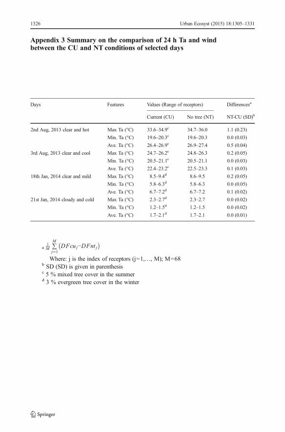
Appendix 3 Summary on the comparison of 24 h Ta and windbetween the CU and NT conditions of selected days

a1M ∑

M

j¼1DFcuj−DFnt j� �

Where: j is the index of receptors (j=1,…, M); M=68b SD (SD) is given in parenthesisc 5 % mixed tree cover in the summerd 3 % evergreen tree cover in the winter

Days Features Values (Range of receptors) Differencesa

Current (CU) No tree (NT) NT-CU (SD)b

2nd Aug, 2013 clear and hot Max Ta (°C) 33.6–34.9c 34.7–36.0 1.1 (0.23)

Min. Ta (°C) 19.6–20.3c 19.6–20.3 0.0 (0.03)

Ave. Ta (°C) 26.4–26.9c 26.9–27.4 0.5 (0.04)

3rd Aug, 2013 clear and cool Max Ta (°C) 24.7–26.2c 24.8–26.3 0.2 (0.05)

Min. Ta (°C) 20.5–21.1c 20.5–21.1 0.0 (0.03)

Ave. Ta (°C) 22.4–23.2c 22.5–23.3 0.1 (0.03)

18th Jan, 2014 clear and mild Max Ta (°C) 8.5–9.4d 8.6–9.5 0.2 (0.05)

Min. Ta (°C) 5.8–6.3d 5.8–6.3 0.0 (0.05)

Ave. Ta (°C) 6.7–7.2d 6.7–7.2 0.1 (0.02)

21st Jan, 2014 cloudy and cold Max Ta (°C) 2.3–2.7d 2.3–2.7 0.0 (0.02)

Min. Ta (°C) 1.2–1.5d 1.2–1.5 0.0 (0.02)

Ave. Ta (°C) 1.7–2.1d 1.7–2.1 0.0 (0.01)

1326 Urban Ecosyst (2015) 18:1305–1331

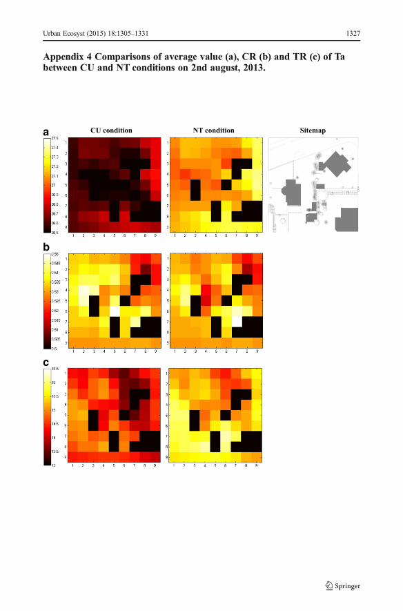
Appendix 4 Comparisons of average value (a), CR (b) and TR (c) of Tabetween CU and NT conditions on 2nd august, 2013.

SitemapCU condition NT conditiona

b

c

Urban Ecosyst (2015) 18:1305–1331 1327

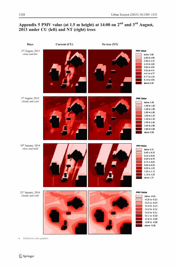
Appendix 5 PMV value (at 1.5 m height) at 14:00 on 2nd and 3rd August,2013 under CU (left) and NT (right) trees

Days Current (CU) No tree (NT)

2nd August, 2013

clear and hot

3rd August, 2013

cloudy and cool

18th January, 2014

clear and mild

21st January, 2014

cloudy and cold

Definition: color graphics

1328 Urban Ecosyst (2015) 18:1305–1331

Appendix 6 PMV value (at 1.5 m height) at 22:00 on 2nd and 3rd August,2013 under CU (left) and NT (right) conditions

Days Current (CU) No tree (NT)

2nd

August, 2013

clear and hot

3rd

August, 2013

cloudy and cool

18th

January, 2014

clear and mild

21st January, 2014

cloudy and cold

Urban Ecosyst (2015) 18:1305–1331 1329

Open Access This article is distributed under the terms of the Creative Commons Attribution License whichpermits any use, distribution, and reproduction in any medium, provided the original author(s) and the source arecredited.

References

Akbari H (2002) Shade trees reduce building energy use and CO2 emissions from power plants. Environ Pollut116:S119–126. Retrieved from http://www.ncbi.nlm.nih.gov/pubmed/11833899

Akbari H, Pomerantz M, Taha H (2001) Cool surfaces and shade trees to reduce energy use and improve airquality in urban areas. Sol Energy 70(3):295–310. doi:10.1016/S0038-092X(00)00089-X

Berry R, Livesley SJ, Aye L (2013) Tree canopy shade impacts on solar irradiance received by building walls andtheir surface temperature. Build Environ 69:91–100. doi:10.1016/j.buildenv.2013.07.009

Bonan GB (2002) Ecological climatology : concepts and applications (p. 678 pp). Cambridge University Press,Cambridge

Bruse M (2010) ENVI-met 3.1: Updated model overview. Bochum, Germany. Retrieved from http://www.envi-met.com

Chen WY, Jim CY (2008) Assessment and valuation of the ecosystem services provided by urban forests. In:Carreiro MM, Song YC, Wu J (eds) Ecology, planning, and management of urban forests: internationalperspectives. Springer, New York, pp 53–83

Emmanuel R, Rosenlund H, Johansson E (2007) Urban shading – a design option for the tropics? A study inColombo, Sri Lanka. J Climatol 27:1995–2004. doi:10.1002/joc.1609

Fahmy M, Sharples S, Eltrapolsi A (2009) Dual stage simulations to study the microclimatic effects of trees onthermal comfort in a residential building, Cairo, Egypt. In: Eleventh International IBPSA Conference.Building Simulation, Glasgow, pp 1730–1736

Frelich LE (1992) Predicting dimensional relationship for twin cities shade trees. Department of ForestResources, University of Minnesota, St. Paul, MN

Hedquist BC, Brazel AJ (2014) Seasonal variability of temperatures and outdoor human comfort in Phoenix,Arizona, U.S.A. Build Environ 72:377–388. doi:10.1016/j.buildenv.2013.11.018

Heisler GM, Grant RH (2000) Ultraviolet radiation in urban ecosystems with consideration of effects on humanhealth. Urban Ecosyst 4:193–229

Huang L, Li J, Zhao D, Zhu J (2008) A fieldwork study on the diurnal changes of urban microclimate in fourtypes of ground cover and urban heat island of Nanjing, China. Build Environ 43(1):7–17. doi:10.1016/j.buildenv.2006.11.025

ISO 7726 (1998) Ergonomics of the thermal environment - instruments for measuring physicalquantities. International Standard Organization, Geneva

Kuye A, Jagtap SS (1992) Analysis of solar radiation data for port harcourt, Nigeria. Sol Energy 49(2):135–145Lalic B, Mihailovic DT (2004) An empirical relation describing Leaf-Area Density inside the forest for

environmental modeling. J Appl Met Clim 43(4):641–645Matzarakis A, Mayer H (1998) Investigations of urban climate’s thermal component in Freiburg, Germany. In:

Preprints second urban environment symposium - 13th conference on biometeorology and aerobiology.American Meteorological Society, Albuquerque, pp 140–143

Mcpherson EG, Herrington LP, Heisler GM (1988) Impacts of vegetation on residential heating and cooling.Energy Build 12:41–51

McPherson EG, Simpson JR, Livingston M (1989) Effects of three landscape treatments on residential energyand water use in Tucson, Arizona. Energy Build 13:127–138

Middel A, Häb K, Brazel AJ, Martin CA, Guhathakurta S (2014) Impact of urban form and design on mid-afternoon microclimate in Phoenix Local Climate Zones. Landsc Urban Plan 122:16–28. doi:10.1016/j.landurbplan.2013.11.004

MA - Millennium Ecosystem Assessment (2005) Ecosystems and human well-being: synthesis. Island Press,Washington

Morakinyo TE, Balogun AA, Adegun OB (2013) Comparing the effect of trees on thermal conditions of twotypical urban buildings. Urban Clim 3:76–93. doi:10.1016/j.uclim.2013.04.002

Park M, Hagishima A, Tanimoto J, Narita K (2012) Effect of urban vegetation on outdoor thermal environment:field measurement at a scale model site. Build Environ 56:38–46. doi:10.1016/j.buildenv.2012.02.015

Peng L, Jim C (2013) Green-roof effects on neighborhood microclimate and human thermal sensation. Energies6(2):598–618. doi:10.3390/en6020598

1330 Urban Ecosyst (2015) 18:1305–1331

Shahidan MF, Jones PJ, Gwilliam J, Salleh E (2012) An evaluation of outdoor and building environment coolingachieved through combination modification of trees with ground materials. Build Environ 58:245–257. doi:10.1016/j.buildenv.2012.07.012

Skoulika F, Santamouris M, Kolokotsa D, Boemi N (2014) On the thermal characteristics and the mitigationpotential of a medium size urban park in Athens, Greece. Landsc Urban Plan 123:73–86. doi:10.1016/j.landurbplan.2013.11.002

Taha H, Akbari H, Rosenfeld A (1991) Heat island and oasis effects of vegetative canopies: micro-meteorological field-measurements. Theor Appl Climatol 44:123–138

Wang Y, Bakker F, de Groot R, Wörtche H (2014) Effect of ecosystem services provided by urban greeninfrastructure on indoor environment: a literature review. Build Environ 77:88–100. doi:10.1016/j.buildenv.2014.03.021

Willmott CJ (1981) On the validation of models. Phys Geogr 2:184–194

Urban Ecosyst (2015) 18:1305–1331 1331