effects of window size and shape on accuracy of subpixel ...mln/ltrs-pdfs/tp3331.pdf · accuracy of...
TRANSCRIPT

NASATechnicalPaper3331
September 1993
Effects of WindowSize and Shape onAccuracy of SubpixelCentroid Estimationof Target Images
Sharon S. Welch

NASATechnicalPaper3331
1993
Effects of WindowSize and Shape onAccuracy of SubpixelCentroid Estimationof Target Images
Sharon S. WelchLangley Research CenterHampton, Virginia

Abstract
A new algorithm is presented for increasing the accuracy of subpixelcentroid estimation of (nearly) point target images in cases where thesignal-to-noise ratio is low and the signal amplitude and shape vary fromframe to frame. In the algorithm, the centroid is calculated over a datawindow that is matched in width to the image distribution. Fourieranalysis is used to explain the dependency of the centroid estimateon the size of the data window, and simulation and experimentalresults are presented which demonstrate the e�ects of window size fortwo di�erent noise models. The e�ects of window shape have alsobeen investigated for uniform and Gaussian-shaped windows. Thenew algorithm has been developed to improve the dynamic range of aclose-range photogrammetric tracking system that provides feedback forcontrol of a large gap magnetic suspension system (LGMSS).
Introduction
Centroid-estimation algorithms have long beenused in digital imaging to locate target images tosubpixel accuracies. Applications of centroid esti-mation include star tracking (ref. 1), point and edgedetection for machine vision (ref. 2), close-rangephotogrammetry (ref. 3), and motion analysis. Thee�ects of sampling and noise on the accuracy of thecentroid estimate for point source images, images ofextended sources, and edge detection have been ana-lyzed previously and documented by several authors(refs. 4 to 8). The systematic errors due to under-sampling that have been described for centroid esti-mation are common to all interpolation algorithmsand have been analyzed from the point of view ofperforming image reconstruction (refs. 9 and 10). Inthese previous analyses, experimental approaches aswell as analytical approaches based on Fourier tech-niques have been used to quantify the errors due tonoise, quantization, and sample spacing. To date,the e�ect of window size on the accuracy of subpixelcentroid estimation has been limited to a qualitativeanalysis derived from experiments that measured theerror in centroid estimation as a function of di�erentN -point algorithms (ref. 4).
In this paper, Fourier techniques are used to an-alyze the dependency of the systematic error on win-dow size. In addition, the e�ects of window sizeand shape on subpixel centroid-estimation accuracyin the presence of noise are studied. It is shown thatthere can be an advantage to using a shaped win-dow for centroid estimation of point target images forsignals that vary in amplitude and width, providedthe pixel-to-pixel noise is independent of signal am-plitude. A brief review of the e�ects of the opticalpoint spread function (PSF), target size, and sam-ple spacing on systematic error is provided in order
to compare and contrast these e�ects with those at-tributable to the data window. Quantization e�ects,however, are not addressed in this paper.
In many applications involving centroid estima-tion, the signal shape and amplitude are either con-trollable or �xed. In these cases, the optimum sam-ple spacing and window size relative to the targetimage distribution are known a priori, and a correc-tion can be applied for systematic errors (ref. 7). Inother applications where the noise is small or the im-age is averaged over several frames, a larger window(relative to the distribution) can be used in the cen-troid calculation. This eliminates systematic errorsarising because of truncation of the signal. In theapplication discussed in this paper, centroid estima-tion is used to locate images of point targets along alinear charge-coupled device (CCD) detector, wherethe signal-to-noise ratio is small and, because the tar-gets are moving, the (one-dimensional) images varyin size and amplitude. For these reasons, it is notpossible to apply a correction for the systematic er-rors or to calculate the centroid using a large �xeddata window.
The application discussed herein is the opticalmeasurement system (OMS) for the large gap mag-netic suspension system (LGMSS) (�g. 1). In theOMS, small infrared light-emitting diode (LED) tar-gets have been embedded in the top surface of arigid cylindrically shaped element that contains apermanent magnet core. The element is magneticallylevitated above a planar array of electromagnets.Sixteen linear CCD cameras arranged in pairs arelocated symmetrically about and above the levitatedcylinder. A total of eight targets are located alongthe top surface of the cylinder (�g. 2), and the tar-gets are multiplexed in time for target identi�cation.Triangulation techniques are used to determine the

position and attitude of the levitated cylinder fromthe locations of the projected target images in the16 cameras. The position and attitude informationis supplied to the electromagnet controller to stabi-lize levitation of the cylinder and to control motionin six degrees of freedom.
The position and attitude of the cylinder are de-termined using weighted least squares. An estimateof the error in each computed centroid value is passedalong with the centroid value and is used to estab-lish a weighting factor for the particular camera mea-surement. In order to achieve the required accuracyin the estimate of position and attitude, it is neces-sary to locate the centroids of at least 6 of the targetimages to 1/15 of a pixel in a minimum of 12 of the16 cameras. As the cylinder, and hence each tar-get, moves over the �eld of view, both the amplitudeand the width of the target images vary (�g. 3). Ifthe centroid location of a target image is determinedwith a �xed window size (which is the same for all16 cameras), and the window size is optimum forthose image distributions falling in the midrange ofpossible values, then as the target images vary in am-plitude and width, the error in the centroid estimategrows for those images for which the distribution fallsoutside the midrange. Thus, with a �xed windowsize, the accuracy of the centroid estimate falls o� be-cause of noise or systematic error, and the accuracyof the position and attitude estimate correspondinglydecreases.
In order to increase the dynamic range of thesystem, an algorithm has been developed to adjustthe width of the centroid window as the light in-tensity distribution of the image varies. This algo-rithm provides the minimum error in centroid esti-mation over the maximum range of signal amplitudeand shape. This paper analyzes the dependency ofsystematic and noise-induced errors on the size andshape of the data window. Experimental results arepresented and compared with the results of numericalsimulations.
The following analysis is limited to one spatial di-mension. It is assumed that the PSF of the imagingoptics can be approximated by a Gaussian function.Because a two-dimensional Gaussian function is sep-arable in x and y, the results of the one-dimensionalanalysis can readily be extended to two dimensions.
Symbols and Abbreviations
b half-width of Gaussian distributionused to simulate the optical pointspread of the imaging optics
comb(x=xs) sampling function
f(x) light intensity distribution of one-dimensional target image
F (�) Fourier transform of f(x)
eF (�) = F (�)R(�)
FRW = FR * W
FSW(�) Fourier transform of fSW(x)
F 0
SW(�) �rst derivative of FSW(�) withrespect to �
fSW(x) sampled and windowed version off(x)
g(x� xo) one-dimensional light intensitydistribution of target located at xo
H(�) general function of �
N number of pixels corresponding tohalf the window width
PSF(x) point spread function of imagingoptics
R(�) Fourier transform of r(x)
r(x) pixel response function
T (�) general function of �
W (�) Fourier transform of w(x)
w(x) window function
x spatial variable
�x centroid of continuous one-dimensional light intensitydistribution
xc amount by which f(x) is shiftedwith respect to the sampling grid
xp pixel location of the peak signal
xs sample spacing
�xSW centroid of fSW(x)
�c systematic error, �x� �xSW
�; �; � variables of integration
Abbreviations:
CCD charge-coupled device
LED light-emitting diode
rms root-mean-square
SNR = Peak signalStandard deviation of background signal
A prime on a symbol denotes the �rst derivative.An asterisk used as an operational sign denotes con-volution of the quantities.
2

E�ect of Window Size on Systematic
Error
The objective is to produce a minimum errorestimate of the centroid of a one-dimensional lightintensity distribution corresponding to a (nearly)point target image. The target image will havebeen sampled and only a portion of the sampleddistribution (those points lying within the window)will have been used in the calculation. By de�nition,the centroid of the continuous one-dimensional lightintensity distribution is given by
�x =
R1
�1
xf(x) dxR1
�1
f(x) dx(1)
where �x is the centroid, f(x) is the light intensitydistribution of the image, and x is the position. Thisequation may be expressed in terms of F (�), theFourier transform of f(x), as
�x =
�dF (�)=d�
�2�iF (�)
��=0
(2)
where
F (�) =
Z1
�1
f(x) exp(�2�i�x) dx (3)
The e�ect of using only a portion of the imagedistribution, that is, of placing a window about thedistribution, is to spread the energy in the spectrumof F (�) into higher frequencies. This e�ect is shownin �gure 4. When the image distribution is bothwindowed and sampled, as it is in practice, the widthof the window relative to the width of f(x) and thesample spacing is important.
In a CCD array, an image is sampled at discreteintervals with an array of detectors or pixels. Eachpixel has a response that is spatially distributed overthe width of the pixel. If f(x) is the function thatrepresents the continuous light intensity distributionof the image, then sampling with a CCD array canbe modelled mathematically as a convolution of f(x)with a function r(x), which represents the spatialresponse of each pixel, followed by a multiplicationof the resulting product with the sampling functioncomb(x=xs), where
1
xscomb(x=xs) =
1Xn=�1
�(x� nxs)
and xs is the sample spacing of the pixels. This con-volution and multiplication results in a sampled data
set that is of in�nite extent. In order to reproduce thereal data set, which is of limited extent, the sampledfunction is multiplied by a window function w(x) of�nite width. If the sampled and windowed functionis de�ned as fSW (x), then
fSW = (f � r)
�1
xscomb
�w (4)
where the asterisk denotes the convolution (pp. 284and 285 of ref. 11). From equations (3) and (4) itfollows that the Fourier transform of fSW(x) is
FSW = eF � comb �W
= (eF �W ) � comb
where
comb =1X
n=�1
�
�� �
n
xs
�
and eF = FR
Thus,
FSW(�) =1X
n=�1
FRW
�� �
n
xs
�(5)
whereFRW = eF �W (6)
Equation (5) shows that the spectrum of thesampled and windowed function is the sum of theindividual spectra FRW repeated at intervals of1=xs. Figure 5 shows a representative sampled andwindowed function fSW(x) and the correspondingFourier transform FSW(�). As for the continuousdistribution case, placing a window about the imagedistribution can broaden FRW . When the image isboth windowed and sampled this spread can resultin energy spillover from neighboring transforms. Ifthe window width is too small relative to the widthof the signal and the sample spacing, then system-atic error is introduced into the centroid estimate asenergy from higher orders spills into FRW(0).
Before the speci�c form of the error introducedby the data window is discussed, the e�ects of theoptical PSF, pixel response function, and target sizeare brie y reviewed in order to distinguish betweenthose errors that are due to undersampling and thoseerrors that are due to the �nite extent of the data.
A Review of E�ects of Optical PSF, Pixel
Response Function, and Target Size
As has been shown previously (refs. 4, 7, 9,and 10), the form of the subpixel error in centroid
3

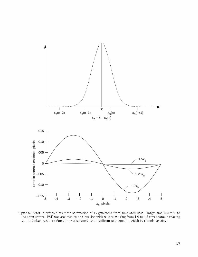
estimation and image reconstruction due to under-sampling is a sinusoidal function of the position ofthe \true" centroid or image location with respect tothe sample grid (�g. 6). The magnitude of this erroris a function of the widths of the optical PSF, pixelresponse function, and target.
In a digital imaging system, the optical PSFdescribes the degree to which the target image isblurred because of the limits of di�raction in theimaging optics. Provided the imaging optics are shiftinvariant, then the light intensity distribution of theimage f(x� xo) is the convolution of g(x�xo) withthe PSF of the imaging optics, where g(x � xo) isthe light intensity distribution of the true target andxo is the location of the centroid of the distribution.(See pp. 335 and 336 of ref. 11.)
Because the optics tend to blur, or smear outthe image of the target, the PSF has an inversee�ect on the Fourier transform of the image. Thatis, the Fourier transform of the blurred image isnarrower than the Fourier transform of the trueimage of the target. For this reason, as shown inreferences 4 and 6 to 8, the systematic error incentroid estimation, or image reconstruction, due toundersampling decreases as the width of the PSF ofthe imaging system increases.
Similarly, the pixel response function r(x) spreadsthe sampled image distribution. This spreading isshown in equation (4), where r(x) is convolved withf(x), or equivalently in equation (6), where F (�)is multiplied by R(�). For the linear CCD arraydetector that was used to generate the experimental
results discussed in this paper, the width of the pixelresponse function is approximately equal to 0.8xs.
The size of the target also a�ects the amplitudeof the undersampling error. Typically, the larger thetarget relative to the sample spacing, the smallerthe systematic error. However, the amplitude of theundersampling error does not decrease monotonicallywith increasing target width. Rather, for a �xed pixelresponse function, if the amplitude of the error isplotted as a function of target size, then the resultinggraph shows this amplitude to be modulated period-ically with target size (refs. 5 and 8). This period-icity can be understood by looking at the graphs of�gure 7, wherein simulated functions f(x) and F (�)are plotted for two di�erent target widths, xs and 4xs(uniform amplitude). The PSF (�g. 7 (a)) is assumedto be of the form
PSF(x) = exp
"��
�x
bxs
�2#
(7)
As is evident in the graphs of �gures 7(b) to 7(d), ifthe target is uniform in intensity and has sharp dis-continuities at the edges, then the Fourier transformof the true target image looks like a sinc function(�g. 7(d)). As the width of the target changes for a�xed PSF and pixel response function, the side lobesmove relative to zero frequency. For some target sizesand PSF's, F (�) and F 0(�) are zero; for others, F 0(�)is between zero and a peak of the side lobes. Theresult of this is that the amplitude of the sinusoidalerror as a function of target size is modulated in aperiodic fashion that is determined by the ratio ofthe width of the target to the sample spacing.
Centroid-Estimation Error for Sampled and Windowed Function
From equation (2), the estimate of the centroid of the sampled and windowed function fSW(x) is
�xSW =F 0
SW(0)
�2�iFSW(0)(8)
With the systematic error �c de�ned as the di�erence between �x and �xSW, then from equations (2) and (8)
�c = �x� �xSW = �1
2�i
"F 0(0)
F (0)�
F 0
SW(0)
FSW(0)
#(9)
4

Substituting equation (5) for FSW (�) yields
�c = �1
2�i
2664F
0(�)
F (�)�
(d=d�)1P
n=�1FRW (� � (n=xs))
1Pn=�1
FRW (� � (n=xs))
3775�=0
(10)
Using the approach introduced in reference 7, and assuming that the distribution of the target image is an
even function about a point that is shifted an amount xc with respect to the sampling grid, results in
f(x) = fe(x� xc)
and
F (�) = exp(�2�ixc�)Fe(�)
Carrying this analysis further, the e�ect of the window on the Fourier transform F (�) is, as shown by
equation (6), a convolution of the Fourier transform of the window function W (�) with eF (�), or
FRW = eF �W =hexp(�2�ixc�)eFe
i�W =
Z1
�1
exp(�2�ixc�)eFe(�)W (� � �) d� (11)
To see the e�ect of the window on the error �c, we return now to equation (10) and solve for F 0RW(�) using
equation (11) and the following relationship:
Z1
�1
T (�)H(� � �) d� =
Z1
�1
T (� � �)H(�) d�
This yields
FRW(�) =
Z1
�1
exp [�2�ixc(� � �)] eFe(� � �)W (�) d�
and
F 0RW(�) =d
d�
Z1
�1
exp [�2�ixc(� � �)] eFe(� � �)W (�) d�
= �2�ixc
Z1
�1
exp [�2�ixc(� � �)] eFe(� � �)W (�) d�
+
Z1
�1
exp[�2�ixc(� � �)]eF 0e(� � �)W (�) d�
Plugging these values for FRW(�) and F 0RW(�) into equation (10), setting � = 0, and cancelling like terms in
the numerator and denominator leaves
�c =1
2�i
1Pn=�1
�R1
�1
exp f�2�ixc[��� (n=xs)]g eF 0e[�� � (n=xs)]W (�) d��
1Pn=�1
�R1
�1
exp f�2�ixc[��� (n=xs)]g eFe[�� � (n=xs)]W (�) d�� (12)
If we assume that the window is an odd number of pixels, then W (�) is an even function. Furthermore, if
one makes the assumption that the pixel response function is symmetric about the center of the pixel, then
5

R(�) is also an even function. Rearranging terms in the numerator and denominator of equation (12) and
realizing that eF 0
e is an odd function yields
�c =1
2�
0BB@�
R1
�1
sin(2�xc�)eF 0e(�)We(�) d� + 21Pn=1
nR1
�1
sin(2�xc�)eF 0e(�)We[(n=xs)� �] d�o
R1
�1
cos(2�xc�)eFe(�)We(�) d�+ 21Pn=1
nR1
�1
cos(2�xc�)eFe(�)We[(n=xs)� �] d�o1CCA (13)
where Z1
�1
cos(2�xc�)eF 0e(�)We(�) d� = 0
and Z1
�1
sin(2�xc�)eFe(�)We(�) d� = 0
because the integral of an odd function times an even function evaluated over even limits is zero. The �rst
integral in the denominator of equation (13) is generally much larger than the second integral, and therefore
�c �1
2�
0BB@�
R1
�1
sin(2�xc�)eF 0e(�)We(�) d� + 21Pn=1
nR1
�1
sin(2�xc�)eF 0e(�)We[(n=xs) � �] d�o
R1
�1
cos(2�xc�)eFe(�)We(�) d�
1CCA (14)
When the window is large, We(�)! �(�) and equation (14) reduces to
�c �1
�
1Pn=1
sin(2�xcn=xs)eF 0e(n=xs)eFe(0)
Because of the frequency cuto� of the optics, the n = 1 term dominates. Thus, the form of the systematic
error in this case is sinusoidal with an amplitude proportional to eF 0e(1=xs).However, when the width of the window is approximately the same as the width of the image distribution,
the convolution integrals of equation (14) spread each of the individual FRW spectra and terms higher than
the �rst become signi�cant. As a result, the form of the subpixel error changes from a pure sinusoid to one
period of a sawtooth plot (�g. 8). The sawtooth form corresponds to the systematic error that arises because of
truncation of the signal. The amplitude of this error is now a function of the width of the window in addition
to the widths of the pixel response function, the PSF, and the target.
A simulation was constructed to study the relationship between the shape and width of the window and
the systematic error in centroid estimation. In all the simulations discussed herein, the target was assumed to
be a point source, the PSF was assumed to be that given in equation (7), and the pixel response function was
assumed to be uniform and of width xs. Two di�erent-shaped windows were simulated: (1) a uniform window,
de�ned by
w(x) =
�1 (xp �Nxs < x < xp+Nxs for N = 1; 2; : : :)0 (Otherwise)
and (2) a Gaussian-shaped window de�ned by
w(x) =
�exp[��(x� x2p)=(2Nxs)
2] (xp� 2Nxs < x < xp+ 2Nxs for N = 1; 2; : : :)
0 (Otherwise)
where xp is the pixel location of the peak signal. The functions w(x) and corresponding Fourier transform
W (�) for the uniform and Gaussian-shaped windows are shown for comparison purposes in �gure 9. Note that
the Fourier transforms for both windows have a zero at approximately the same location. The width of the
6

Gaussian-shaped window has been chosen to provide a similar shape in frequency space to that of the uniform
window. In addition, the error due to undersampling has been made negligibly small. Provided b � 1:25xs,
which was true for the cases that were simulated, the maximum error due to undersampling is less than 0.002
times the pixel spacing.
In �gure 10, the simulation results show the predicted peak amplitude of the subpixel systematic error as
a function of the ratio N=b for the two di�erent-shaped windows. These results show that using a Gaussian-
shaped window reduces the systematic error. The systematic error due to windowing goes to zero with the
Gaussian-shaped window for values of N=b greater than approximately 1.0 and with the uniform window for
values of N=b greater than approximately 2.5.
E�ects of Window Size and Shape on
Noise-Induced Error
In order to understand the e�ects of window sizeand shape on centroid-estimation error in the pres-ence of noise, a simulation was constructed. Twodi�erent noise models were simulated. In one, thenoise was modelled as a mean zero Gaussian ran-dom variable, independent of signal amplitude andindependent for each pixel along the array. In theother, the noise was modelled as being proportionalto the square root of the signal amplitude, where theproportionality factor was modelled as a mean zeroGaussian random variable. The reasons for selectingthese two noise models are the following. Often inimaging applications the target signal is small rela-tive to the background light, and the noise is con-sidered to be background limited photon shot noise(BLIP). This case is simulated by the noise modelin which the noise is independent of the signal andindependent pixel to pixel. The other case closelyapproximates the characteristics of the sensor noisein the OMS.
Equation (7) was used to mathematically modelthe PSF of the optics. The source was modelled as adelta function with a peak signal of 1.0. A constantbackground signal was added to the target signalprior to addition of the noise. When the centroid wasestimated, the values at the endpoints of the windowwere averaged, and this average value was subtractedfrom each signal value. This process simulated thethreshold technique that is used on the OMS.
Simulations were run to determine the subpixelbias error and the standard deviation of the signalat any single subpixel position. To calculate the biaserror, an average centroid estimate was calculated ateach subpixel position and subtracted from the truecentroid location. The average centroid estimate wastaken to be the mean of 25 samples. The standarddeviation of the centroid estimate at each subpixellocation was also calculated.
The results of this simulation analysis are shownin �gures 11 to 13. In �gures 11(a) to 11(d), the av-erage error over a single pixel is plotted as a functionof xc for representative samples of each combinationof noise model and window shape. In �gures 12(a)and 12(b), the rms value of the bias error over a sin-gle pixel is plotted as a function of the ratio N=b forthe uniform window and the Gaussian-shaped win-dow with the pixel-to-pixel noise independent. Therms error over the range �0:5 < xc < 0:5 is de�nedas
rms =
vuut 1
P
PXn=1
(True centroid� Predicted centroid)2
where P is the total number of subpixel positions.In �gures 12(c) and 12(d), similar plots are shownfor the noise proportional to the square root of thesignal amplitude. The di�erent points correspond todi�erent values of SNR in �gures 12(a) and 12(b),where the SNR is de�ned as
SNR =Peak signal
Standard deviation of background signal
and to di�erent standard deviations of the propor-tionality factor in �gures 12(c) and 12(d). Fig-ure 13(a) presents the standard deviations of thecentroid estimates at single subpixel locations as afunction of the SNR for the uniform and Gaussian-shaped windows and noise independent of signal am-plitude. In �gure 13(b), similar graphs are shown forthe uniform and Gaussian-shaped windows and noiseproportional to the square root of signal amplitude.
Four things become apparent from the simula-tion results, the �rst of which has been known forsome time: (1) in the presence of noise, the standarddeviation of the subpixel centroid estimate increaseswith increasing window size, no matter what the win-dow shape or noise model; (2) the optimum windowsize, that is, the window size that minimizes both thebias error and the standard deviation of the centroid
7

estimate, is a function of the SNR and the noisemodel; (3) the optimum window shape is a functionof the noise model; and (4) the subpixel bias errortends toward the sawtooth shape associated with thesystematic truncation error when the noise is pro-portional to the signal. For both noise models, therms value of the bias error increases at a slower ratefor the Gaussian-shaped window than for the uni-form window. However, the magnitude of this erroris greater for the Gaussian-shaped window than forthe uniform window when the noise is proportionalto the square root of the signal amplitude; the errormagnitude for the Gaussian-shaped window is lessthan that for the uniform window when the pixel-to-pixel noise is independent and mean zero Gaussian.It follows from this that in order to determine anoptimum window size (and shape) for point targettracking, the SNR and noise process must be known.
Experimental Results
Experiments were run to verify the results pre-dicted by simulation. A single camera was mounteddirectly over an LED target. The target was movedover �0.05 in. in the object plane in 0.0025-in. stepsusing a computer-controlled linear stage and imagedwith the camera (�g. 14). The displacement of thestage was measured using a laser interferometer toapproximately 0.0001 in. Since the magni�cation fac-tor for the camera was approximately 0.1, it was pos-sible to resolve the displacement of the target in theimage plane to better than 1/20 of a pixel. The cen-troid of the projected target image was calculatedas the average of the centroid estimates obtained for100 target images acquired at each location of thestage. A straight line was �t through the average cen-troid estimates as a function of the measured stageposition. The bias error was then determined to bethe di�erence between the straight-line �t and theaverage centroid estimate at each location.
Figures 15(a) and 15(b) show the bias errors fora uniform window and a Gaussian-shaped window.In �gure 15(a) (for the uniform window), the largeramplitude error corresponds to N = 4 and thesmaller amplitude error corresponds to N = 6. In�gure 15(b) (for the Gaussian-shaped window), thelarger amplitude error corresponds to N = 5 andthe smaller amplitude error corresponds to N = 15.The image distribution for which the centroid wasestimated is that shown in �gure 16 and was the samefor all N . Assuming a point target, the half-widthof the distribution shown in �gure 16 corresponds tob � 6:0. The jitter that is apparent in the data isthe result of the noise model and the thresholdingtechnique discussed previously.
In order to determine the relationship betweenthe signal SNR, window size and shape, and accu-racy, the experiment described above was repeatedfor di�erent sensor integration times. Figure 17presents the rms values of the bias error (over 9 cy-cles) for di�erent SNR's and window widths. Fig-ure 17(a) shows the results obtained with a uniformwindow, and �gure 17(b) shows the results obtainedwith a Gaussian-shaped window.
In addition to the bias error, the standard de-viation of the centroid estimate at a single positionof the stage was measured. These results are shownin �gure 18. As expected, the standard deviation ofthe centroid estimate increases with increasing win-dow size. The increase in the standard deviationagain at small window sizes is believed to result fromthresholding. As the window size decreases to thepoint where the signal is truncated, those pixels at ei-ther edge of the window have greater noise associatedwith them. When the threshold is set as the averageof the signals from these two pixels and subtractedfrom the signal at each pixel within the window, therandom error in the estimate of the centroid is in-creased. Therefore, the variation from sample tosample increases.
From the above results, the uniform windowshape is optimum for centroid estimation in the op-tical tracking system. Furthermore, N=b � 1:5 is theoptimum ratio of window width to width of the targetimage distribution for SNR's from about 50 to 100.This ratio of window size to distribution width pro-vides the minimum total error, where the total erroris the sum of the rms value of the bias error and thestandard deviation of the centroid estimate.
Centroid-Estimation Algorithm
A owchart of the centroid-estimation algorithmis shown in �gure 19. The subpixel centroid estimateis calculated in the following way. During tracking, asearch is made for the peak pixel location of each tar-get prior to computation of the centroid. The pixellocation of peak light intensity is stored and usedto set up a window of 81 pixels centered about thepeak. Each pixel has a slightly di�erent response,that is, a slightly di�erent gain and zero point. Priorto computation of the centroid, the values of lightintensity are corrected for pixel nonuniform respon-sivity and the background light level is subtractedfor pixels falling within the window. A second coarsesearch for the peak intensity is then performed overthe corrected light intensity values.
Before the centroid is estimated, the width of thedistribution is determined by computing the second
8

moment of the target image distribution. The secondmoment is calculated as
�� =
xp+15P
n=xp�15
n2I(n)
xp+15P
n=xp�15
I(n)
� �x2
where �x is the centroid of the distribution calculatedover �15 pixels centered about the peak, I(n) is thedigital value of the light intensity for pixel n, and xpis the pixel location of the peak signal.
The value of N used in the centroid calculationis equal to the nearest integer value of the secondmoment �� plus one pixel. The subpixel centroidestimate is calculated as
�xsw =
xp+NP
n=xp�N
nI(n)
xp+NP
n=xp�N
I(n)
Figure 20 shows the subpixel bias error from the useof the centroid-estimation algorithm that adjusts thewindow size; the window shape is uniform. Figure 21shows the standard deviations of the centroid esti-mate for a uniform window of variable width anda uniform window with a �xed width of N = 14.The value of N = 14 was chosen as the size requiredto minimize the systematic error for the maximumsignal obtained during tracking with the OMS. Themaximum signal has an SNR of approximately 200.Adjusting the window size to match the width of thedistribution minimizes the systematic error as well asthe standard deviation of the centroid estimate overa wider range of SNR's than does using a window of�xed size.
Conclusions
The e�ects of window size and shape on the ac-curacy of subpixel centroid estimation have beenpresented. Two di�erent noise models and win-dow shapes have been studied. The shapes includea uniform window and a Gaussian-shaped window.The noise models studied include random mean zeroGaussian, independent pixel to pixel and indepen-dent of signal amplitude, and noise proportional tothe square root of the signal amplitude.
Fourier analysis has been used to determine theform and magnitude of the systematic error dueto windowing. It has been shown that the formof the subpixel error due to windowing resemblesone period of a sawtooth compared with the puresinusoidal waveform that is obtained when the signalis undersampled. Furthermore, it has been shownthat the magnitude of this systematic error is smallerfor a Gaussian-shaped window than for a uniformwindow.
Simulations have been run to explore the sensitiv-ity of the centroid-estimation algorithm to windowsize and shape in the presence of noise and to deter-mine the window shape and size that minimize theerror. Experiments have been conducted to verifythe behavior predicted by simulation. The results ofthe simulations and experiments revealed the follow-ing: (1) for noise that is proportional to the squareroot of the signal amplitude, the optimum windowshape is uniform, and for noise that is independentof signal amplitude, with a low ratio of peak signal tostandard deviation of background signal (SNR), theoptimum window shape is Gaussian; and (2) match-ing the size of the window to the width of the targetimage distribution improves the accuracy of the cen-troid estimate for both noise models and both win-dow shapes. The optimum ratio of window widthto width of the target distribution is approximately1.5 for the uniform window and noise proportional tosignal amplitude.
The results of the analysis have been used to de-velop a new centroid-estimation algorithm that in-creases the accuracy of subpixel centroid estimationof (nearly) point target images when the noise is pro-portional to signal amplitude and the signal ampli-tude and shape vary from frame to frame. In the al-gorithm, the width of the data window is matched tothe estimated width of the image distribution. Cal-culating the centroid over a window that is matchedin size to the width of the distribution yields a sub-pixel centroid estimate with smaller total error overa wider range of SNR's than that from a calculationwith a window of �xed size. This improvement incentroid estimation has been developed for a pointtarget tracking system in order to increase the dy-namic range of the system.
NASALangley Research Center
Hampton, VA 23681-0001
June 22, 1993
9

References
1. Armstrong, R. W.; and Staley, Douglas A.: A Survey of
Current Solid State Star Tracker Technology. J. Astro-
naut. Sci., vol. 33, no. 4, Oct.{Dec. 1985, pp. 341{352.
2. Bales, JohnW.; and Barker, L. Keith: Marking Parts To
Aid Robot Vision. NASA TP-1819, 1981.
3. El-Hakim, S. F.: Real-Time ImageMetrologyWith CCD
Cameras. Photogramm. Eng. & Remote Sens., vol. 52,
no. 11, Nov. 1986, pp. 1757{1766.
4. Grossman, S. B.; andEmmons,R. B.: PerformanceAnal-
ysis and Size Optimization of Focal Planes for Point
Source Tracking Algorithm Applications. Focal Plane
Methodologies III, Volume 350 of SPIE Proceedings,
J. T. Hall and W. S. Chan, eds., International Soc. for
Optical Engineering, 1983, pp. 94{108.
5. Stanton, Richard H.; Alexander, James W.; Dennison,
Edwin W.; Glavich, Thomas A.; and Hovland, Larry F.:
Optical Tracking Using Charge-Coupled Devices. Opt.
Eng., vol. 26, no. 9, Sept. 1987, pp. 930{938.
6. Cox, J. Allen: Advantages of Hexagonal Detectors and
Variable Focus for Point-Source Sensors. Opt. Eng.,
vol. 28, no. 11, Nov. 1989, pp. 1145{1150.
7. Alexander, Brian F.; and Ng, KimChew: Elimination of
Systematic Error in Subpixel Accuracy Centroid Estima-
tion. Opt. Eng., vol. 30, no. 9, Sept. 1991, pp. 1320{1331.
8. Wittenstein, W.; Fontanella, J. C.; Newbery, A. R.; and
Baars, J.: The De�nition of the OTF and the Measure-
mentofAliasing for SampledImagingSystems. Opt.Acta,
vol. 29, no. 1, 1982, pp. 41{50.
9. Park, Stephen K.; and Schowengerdt, Robert A.: Image
Sampling,Reconstruction, and theE�ectof Sample-Scene
Phasing. Appl. Opt., vol. 21, no. 17, Sept. 1, 1982,
pp. 3142{3151.
10. Park, S. K.; Kaczynski, M.-A.; and Schowengerdt,
R. A.: Modulation-Transfer-Function Analysis for Sam-
pled Image Systems. Appl. Opt., vol. 23, no. 15, Aug. 1,
1984, pp. 2572{2582.
11. Gaskill, Jack D.: Linear Systems, Fourier Transforms,
and Optics. John Wiley & Sons, Inc., c.1978.
10

Levitation andcontrol magnet
Insert and retrievemechanism
OMS sensing units
Suspended element
OMS camera support structure
Figure 1. Optical measurement system (OMS) of large gap magnetic suspension system (LGMSS).
Phototransistor LEDLED
Rechargeable batteries
Permanent magnet coreLED driver electronics
Figure 2. Levitated cylinder with locations of eight LED targets.
11

1357
Target600
500
400
300
200
100
0
-100
Dig
ital s
igna
l am
plitu
de
0 5 10 15 20 25Pixels along array
Figure 3. Digital signals (expanded) corresponding to light intensity distributions for images of targets 1, 3,5, and 7 as viewed from sensor 7 in OMS. All images have been referenced to same peak pixel location tobetter illustrate range of sizes and shapes of sampled image distributions that can be generated by di�erenttargets.
12

f(x)f(x)w(x)
xSpatial frequency
(a) Continuous distribution f(x).
F(ξ)
F*W
ξ0
Spatial frequency
(b) Fourier transform of f(x) multiplied by Fourier transform of window function w(x), uniform window placedsymmetrically about f(x).
Figure 4. E�ect of windowing.
13

fSW(x)
x
0
xs
Spatial frequency
(a) Representative signal.
FSW(ξ)
ξ0
1/xs
Spatial frequency
(b) Fourier transform of signal.
Figure 5. Representative sampled and windowed signal corresponding to point target image and Fouriertransform of this signal.
14
xs(n+1)x
xs(n)xs(n–1)xs(n–2)
_
xc = x – xs(n)_
.015
.010
.005
0
-.005
-.010
-.015-.4-.5 -.3 -.2 -.1 0 .1 .2 .3 .4 .5
xc, pixels
Err
or in
cen
troi
d es
timat
e, p
ixel
s
1.0xs
1.5xs
1.25xs
Figure 6. Error in centroid estimate as function of xc generated from simulated data. Target was assumed to
be point source, PSF was assumed to be Gaussian with widths ranging from 1.0 to 1.5 times sample spacingxs, and pixel response function was assumed to be uniform and equal in width to sample spacing.
15

1.0
.8
.6
.4
.2
0-15 -10 -5 0 5 10 15
x, pixels
Am
plitu
de
(a) Simulated PSF; b = 1:0.
1.0
.8
.6
.4
.2
0-15 -10 -5 0 5 10 15
x, pixels
Nor
mal
ized
am
plitu
de
(b) Simulated target of uniform intensity and width of 4xs.
Figure 7. Simulated digital data for di�erent target widths and corresponding Fourier transforms.
16

1.0
.8
.6
.4
.2
0-15 -10 -5 0 5 10 15
Pixels
Nor
mal
ized
am
plitu
de
(c) Convolution of target from �gure 7(b) with r(x) of width xs.
5
4
2
1
0
-1-15 -10 -5 0 5 10 15
Spatial frequency, pixels-1
Am
plitu
de
3
× 104
(d) Fourier transform of convolution from �gure 7(c).
Figure 7. Continued.
17

1.0
.8
.6
.4
.2
0-15 -10 -5 0 5 10 15
x, pixels
Nor
mal
ized
am
plitu
de
(e) Simulated target of uniform intensity and width of xs.
1.0
.8
.6
.4
.2
0-15 -10 -5 0 5 10 15
x, pixels
Nor
mal
ized
am
plitu
de
(f) Convolution of target from �gure 7(e) with pixel response function of width xs.
Figure 7. Continued.
18

12 000
10 000
6 000
4 000
2 000
0-1.5 -1.0 -.5 0 .5 1.0 1.5
Spatial frequency, pixels-1
Am
plitu
de
8 000
(g) Fourier transform of convolution from �gure 7(f).
Figure 7. Concluded.
19

-.06-.4-.5 -.3 -.2 -.1 0 .1 .2 .3 .4 .5
xc, pixels
Sys
tem
atic
err
or, p
ixel
s
3.02.42.01.3
1.001.251.501.50
N/b b
.6-.6
-.05
-.04
-.03
-.02
-.01
0
.01
.02
.03
.04
.05
.06
.07
Figure 8. Four curves of subpixel error as function of xc for uniform window.
20

1.0
.8
.6
.4
.2
0-15 -10 -5 0 5 10 15
x, pixels
Am
plitu
de
Uniform window
Gaussian-shapedwindow
(a) w(x).
10
8
6
4
2
-4-1.0 -.5 0 .5 1.0
Spatial frequency, pixels-1
Am
plitu
de
0
-2
Uniform window
Gaussian-shapedwindow
(b) W (�).
Figure 9. Representative functions w(x) and W (�) for Gaussian-shaped window and uniform window. N = 5.
21

Gaussian-shaped windowUniform window
.30
.25
.20
.15
.10
.05
Pea
k su
bpix
el e
rror
, pix
els
0 1 2 3 4 5N/b
Figure 10. Peak subpixel error plotted as function of N=b for uniform window and Gaussian-shaped window.
22

.05
.04
.02
0
-.02
-.04
Err
or, p
ixel
s
-.5 -.3 -.1 .1 .3 .5xc
-.2 0 .2 .4-.4-.05
-.03
.03
.01
-.01
(a) Gaussian mean zero noise and uniform window; standard deviation, 0.01.
.05
.04
.02
0
-.02
-.04
Err
or, p
ixel
s
-.5 -.3 -.1 .1 .3 .5xc
-.2 0 .2 .4-.4-.05
-.03
.03
.01
-.01
(b) Gaussian mean zero noise and Gaussian-shaped window; standard deviation, 0.01.
Figure 11. Average subpixel error as function of position xc for combinations of noise model and window shape.N=b = 2:105.
23

.05
.04
.02
0
-.02
-.04
Err
or, p
ixel
s
-.5 -.3 -.1 .1 .3 .5xc
-.2 0 .2 .4-.4-.05
-.03
.03
.01
-.01
(c) Noise proportional to square root of signal amplitude and uniform window; standard deviation, 0.1.
.05
.04
.02
0
-.02
-.04
Err
or, p
ixel
s
-.5 -.3 -.1 .1 .3 .5xc
-.2 0 .2 .4-.4-.05
-.03
.03
.01
-.01
(d) Noise proportional to square root of signal amplitude and Gaussian-shaped window; standard deviation,0.1.
Figure 11. Concluded.
24

0.01.02.03.04.05
Standard deviationof noise
.25
.20
.15
.10
.05
0
rms
of b
ias
erro
r, p
ixel
s
.5 1.0 1.5 2.0 2.5 3.0N/b
(a) Gaussian mean zero noise and uniform window.
0.01.02.03.04.05
Standard deviationof noise
.25
.20
.15
.10
.05
0
rms
of b
ias
erro
r, p
ixel
s
.5 1.0 1.5 2.0 2.5 3.0N/b
(b) Gaussian mean zero noise and Gaussian-shaped window.
Figure 12. Root-mean-square of bias error over single pixel.
25

0.1.2.3.4.5
Standard deviationof proportionality constant
.25
.20
.15
.10
.05
0
rms
of b
ias
erro
r, p
ixel
s
.5 1.0 1.5 2.0 2.5 3.0N/b
(c) Noise proportional to square root of signal amplitude and uniform window.
0.1.2.3.4.5
Standard deviationof proportionality constant
.25
.20
.15
.10
.05
0
rms
of b
ias
erro
r, p
ixel
s
.5 1.0 1.5 2.0 2.5 3.0N/b
(d) Noise proportional to square root of signal amplitude and Gaussian-shaped window.
Figure 12. Concluded.
26

0.01.02.03.01.02.03
Standard deviationof noise
.25
.20
.15
.10
.05
0Sta
ndar
d de
viat
ion
of c
entr
oid
estim
ate,
pix
els
.5 1.0 1.5 2.0 2.5 3.0N/b
UniformUniformUniformGaussianGaussianGaussian
Windowshape
(a) Gaussian mean zero noise.
0.1.2.3.1.2.3
Standard deviationof noise.25
.20
.15
.10
.05
0Sta
ndar
d de
viat
ion
of c
entr
oid
estim
ate,
pix
els
.5 1.0 1.5 2.0 2.5 3.0N/b
UniformUniformUniformGaussianGaussianGaussian
Windowshape
(b) Noise proportional to square root of signal amplitude.
Figure 13. Predicted standard deviations of centroid estimates at any single subpixel position.
27

Figure 14. Experimental setup showing camera mounted overhead of diode and computer-controlled linear stages.
28

.20
.15
0
-.15
Bia
s er
ror,
pix
els
1077 1079 1082 1084 1086Pixel number
1080 1081 1083 10851078-.20
-.10
.10
.05
-.05
N = 4
N = 6
(a) Uniform window.
.20
.15
0
-.15
Bia
s er
ror,
pix
els
1077 1079 1082 1084 1086Pixel number
1080 1081 1083 10851078-.20
-.10
.10
.05
-.05
N = 5
N = 15
(b) Gaussian-shaped window.
Figure 15. Subpixel bias error for uniform and Gaussian-shaped windows.
29

200
150
100
50
Sig
nal a
mpl
itude
, cou
nts
0 10 30 40 60 70Pixel number
5020
Figure 16. Representative target signal, at an integration time of 3 msec, that was used to generate resultsdepicted in �gure 15.
30

237
Integrationtime, msec
.25
.20
.15
.10
.05
0
rms
of b
ias
erro
r, p
ixel
s
3 5 6 7N
4
(a) Uniform window.
237
Integrationtime, msec
.09
.08
.07
.06
.03
.02
rms
of b
ias
erro
r, p
ixel
s
0 5 20 25 30 40N
10 15 35
.04
.05
(b) Gaussian-shaped window.
Figure 17. Experimental rms of bias error as function of window size. Note the di�erence in vertical scalebetween the two plots.
31

3737
Integrationtime, msec
.14
.12
.08
.06
.04
0Sta
ndar
d de
viat
ion
of c
entr
oid
estim
ate,
pix
els
2 4 6 10 12 16N
UniformUniformGaussianGaussian
Windowshape
.10
.02
8 14
Figure 18. Experimental standard deviation of centroid estimate at single position of stage. Integration time
was varied in order to vary e�ective SNR.
32

Start
Read imagedata
Search every thirdpixel for peak
location, PK_LOC
IsPK_LOC>50 or<1999
?
No
Set error flag
Correct data forpixel nonuniformity
Yes
Search ±40 pixelsabout peak for new
peak location
PK_LOC = New peaklocation
N = σ + 1_
Calculate centroid x:_
Calculate second momentσ for ±30 pixelsabout PK_LOC
_
x =_
PK_LOC+N
Σ I(n) n=PK_LOC–N
PK_LOC+N
Σ nI(n) n=PK_LOC–N
Figure 19. Flowchart of centroid-estimation algorithm.
33

.20
.15
0
-.15
Bia
s er
ror,
pix
els
1030 1031 1035 1036Pixel number
1032 1033 1034-.20
-.10
.10
.05
-.05
(a) SNR = 60.
.20
.15
0
-.15
Bia
s er
ror,
pix
els
1030 1031 1035 1036Pixel number
1032 1033 1034-.20
-.10
.10
.05
-.05
(b) SNR = 125.
Figure 20. Subpixel bias error from use of centroid-estimation algorithm that adjusts window size.
34

Fixed widthVariable width
.09
.08
.06
.05
.03
.02Sta
ndar
d de
viat
ion
of c
entr
oid
estim
ate,
pix
els
60 80 100 120 140 160SNR
.07
.04
Figure 21. Standard deviation of centroid estimate versus SNR for uniform window of variable width and �xed
width of N = 14.
35

Figure 14. Experimental setup showing camera mounted overhead of diode and computer-controlled linear
stages.
L-91-16508
1

REPORT DOCUMENTATION PAGEForm Approved
OMB No. 0704-0188
Public reporting burden for this collection of information is estimated to average 1 hour per response, including the time for reviewing instructions, searching existing data sources,gathering and maintaining the data needed, and completing and reviewing the collection of information. Send comments regarding this burden estimate or any other aspect of thiscollection of information, including suggestions for reducing this burden, to Washington Headquarters Services, Directorate for Information Operations and Reports, 1215 Je�ersonDavis Highway, Suite 1204, Arlington, VA 22202-4302, and to the O�ce of Management and Budget, Paperwork Reduction Project (0704-0188), Washington, DC 20503.
1. AGENCY USE ONLY(Leave blank) 2. REPORT DATE 3. REPORT TYPE AND DATES COVERED
September 1993 Technical Paper
4. TITLE AND SUBTITLE
E�ects of Window Size and Shape on Accuracy of SubpixelCentroid Estimation of Target Images
6. AUTHOR(S)
Sharon S. Welch
7. PERFORMING ORGANIZATION NAME(S) AND ADDRESS(ES)
NASA Langley Research CenterHampton, VA 23681-0001
9. SPONSORING/MONITORING AGENCY NAME(S) AND ADDRESS(ES)
National Aeronautics and Space AdministrationWashington, DC 20546-0001
5. FUNDING NUMBERS
WU 590-14-11-02
8. PERFORMING ORGANIZATION
REPORT NUMBER
L-17113
10. SPONSORING/MONITORING
AGENCY REPORT NUMBER
NASA TP-3331
11. SUPPLEMENTARY NOTES
12a. DISTRIBUTION/AVAILABILITY STATEMENT 12b. DISTRIBUTION CODE
Unclassi�ed{Unlimited
Subject Category 35
13. ABSTRACT (Maximum 200 words)
A new algorithm is presented for increasing the accuracy of subpixel centroid estimation of (nearly) pointtarget images in cases where the signal-to-noise ratio is low and the signal amplitude and shape vary fromframe to frame. In the algorithm, the centroid is calculated over a data window that is matched in widthto the image distribution. Fourier analysis is used to explain the dependency of the centroid estimate on thesize of the data window, and simulation and experimental results are presented which demonstrate the e�ectsof window size for two di�erent noise models. The e�ects of window shape have also been investigated foruniform and Gaussian-shaped windows. The new algorithm has been developed to improve the dynamic rangeof a close-range photogrammetric tracking system that provides feedback for control of a large gap magneticsuspension system (LGMSS).
14. SUBJECT TERMS 15. NUMBER OF PAGES
Centroid estimation; Target tracking; Charge-coupled device (CCD) sensors 36
16. PRICE CODE
A0317. SECURITY CLASSIFICATION 18. SECURITY CLASSIFICATION 19. SECURITY CLASSIFICATION 20. LIMITATION
OF REPORT OF THIS PAGE OF ABSTRACT OF ABSTRACT
Unclassi�ed Unclassi�ed Unclassi�ed
NSN 7540-01-280-5500 Standard Form 298(Rev. 2-89)Prescribed by ANSI Std. Z39-18298-102