efficiency analysis of alternative production systems in...

Institute of Landscape Ecology and Resources Management

Division of Landscape Ecology and Landscape Planning

Efficiency analysis of alternative production systems in

Kosovo - an ecosystem services approach

Inaugural Dissertation submitted to the

Faculty 09

Agricultural Sciences, Nutritional Sciences, and Environmental Management

Justus-Liebig-University Giessen

for the degree of

Doctor agricultura (Dr. agr.)

presented by

Iliriana Miftari, Msc.

born in Prishtina, Kosovo

Giessen, February 2017

With permission from the Faculty 09 Agricultural Sciences, Nutritional Sciences, and

Environmental Management,

Justus-Liebig-University Giessen

Dean: Prof. Dr. Klaus Eder

Examination Board:

Supervisor: Prof. Dr. Rainer Waldhardt

Co-supervisor: Prof. Dr. Ernst August Nuppenau

Chair of the Examination

Committee:

Prof. Dr. Dr. habil. Dr. h.c. Annette Otte

SUMMARY

The efficiency estimation and the interpretation of its behavior are of extreme interest for

primary producer in agriculture as well as for policy makers. The efficiency analysis became

very popular with the extensive increase of the resource depletion. It is a technique that measures

output/input ratio of a decision making unit that converts inputs into outputs. In agriculture,

efficiency analysis is crucial to improve competitiveness at sector level through the

improvements of resource utilization by farms and it also serves for evidence based policy

making.

In Kosovo one of the main objectives of Agriculture and Rural Development Plan 2007-2013

and 2014-2020 is to improve competitiveness and the efficiency of primary agricultural

producers and to attain sustainable land use. Regardless of this, there was a lack of studies on

farm efficiency estimation and the productivity changes of the agriculture sector in Kosovo.

Therefore, the conducted study of this thesis focuses on estimation and the analysis of efficiency

at farm level. More specifically, the study aimed estimation of technical, economic, and

environmental efficiency of the farms oriented on tomato, grape and apple production. In

addition, identification of the factors that extensively explain the variation of the efficiency

scores among farms was sought.

The study was based entirely on primary data, collected in three different stages. In the first

stage, a survey using structured questionnaire was conducted with 120 farms which were

distributed equally for each selected production system in the study. This group of data provided

information on demographics and composition of the farm household, employment status,

sources and composition of the farm income, land use, crop production, yields and inputs used.

In the second stage of the study, 304 soil samples were collected at cultivated and uncultivated

farm land. The soil chemical analysis were carried out in order to be able to describe internal soil

nutrition and soil quality for each farm. In the third stage of the research, data describing the

ecological aspect of biodiversity provided by farms was collected.

Descriptive statistics, analysis of variance, statistical tests and correlation coefficients were used

to describe and analyze household and farm characteristics of the three production systems.

Principle Component Analysis and Normative Method were used to aggregate soil chemical

parameters into one index value that described soil quality at farm level. Shannon's Diversity

Index based on the number of cultivated varieties within each crop (tomato, apple and grape) was

used as an indicator for agro-biodiversity provision by each farm.

Farm efficiency scores were obtained using a Data Envelopment Analysis, which is a linear

programming optimization technique that measures relative efficiency of a set of comparable

units. Two different objective functions under constant and variable returns to scale were

estimated for the technical and economic efficiency. At the input oriented model, the objective

function was to minimize the level of all inputs used in the production function while keeping the

output level constant. While, at the output oriented model the objective function is other way

around. The inputs used in the technical and economic efficiency estimation were saplings,

fertilizers, packing, machinery and labor and the sales of tomato, apple and grape yields as an

output. In the second stage of the analysis, truncated regression model was performed to see

which of the farm characteristics were statistically important for efficiency scores variation

among farms. At the environmental efficiency estimation in addition to the aforementioned

inputs and outputs, soil quality and agro-biodiversity were introduced as desirable outputs in the

production function.

In general, the efficiency scores for three different production systems were high, showing that

there was little space for efficiency improvement. On average, tomato farms tend to be more

technical efficient, followed by scale, revenue, and cost allocative efficiency. The lowest average

for this group of farms was on cost efficiency. The input prices played an important role for farm

efficiency, when cost-minimizing objective function was considered.

Farmers oriented in grape production were very scale efficient, followed by technical, revenue

and cost allocative efficiency. Similar to the previous group, the average of cost efficiency score

was the lowest and this can be explained with the differences of market prices for less attractive

vine varieties and more attractive ones. Farmers which were cultivating vine varieties less

attractive for vine processors, had significantly lower price per unit of output and less revenue.

This on the other side increased the costs per unit of output and also decreased the average cost

efficiency score.

Apple farms on average were performing relatively well in terms of technical efficiency which

was the highest on average, followed by revenue efficiency and scale efficiency. Same as for

grape producers, the average cost efficiency score was the lowest, indicating high variations of

the market input and output prices among the farmers.

Factors which were proved to be statistically important in explaining the variation of the

efficiency scores among the farms were household size, farm size and number of cultivated

crops, number of land plots, farmer's education and experience in farming.

On average, the farm efficiency scores increased when environmental variables were introduced

into the model. The distribution of the efficiency scores reallocated farms from lower to the

higher efficiency ranges between technical and environmental efficiency.

In terms of the position in ranking between technical and environmental efficiency estimation,

three different group of farms were found. A group of farms which showed increase in ranking at

environmental efficiency when compared to the technical one. Farms with no difference in

ranking, and a group of farms showing a decrease in ranking at environmental efficiency

compared to the technical efficiency.

Farms which displayed an increase in ranking were mostly farms that improved or maintained

good quality of soil at farm land and good level of agro-biodiversity provision. The second group

of farms showed no difference in ranking, as they were fully efficient in technical and

environmental efficiency estimation. The third group of farms which showed a decrease in

ranking were those farms performing weakly in both technical and environmental efficiency.

This group of farms were also having lower soil quality at farm land and lower agro-biodiversity

when compared to the averages of total sample.

ACKNOWLEDGEMENTS

My special gratitude goes to my first supervisor Prof. Dr. Rainer Waldhardt for his vice advice

and the given great support throughout my study. I also would like to express my great

acknowledgement to my second supervisor Prof. Dr. Ernst August Nuppenau for his valuable

comments on this study.

I am also very thankful to Prof. Dr. Annette Otte and other colleagues for always welcoming me

at the Institute of Landscape Ecology and Resources Management of Giessen University. I also

would like thank committee members Prof. Aurbacher, Prof. Honermeier and Prof. Düring for

the valuation of my PhD thesis.

I want to extend my acknowledgements and being very thankful to Prof. Bernard Del'homme,

Dr. Irina Solovyeva and Dr. Matthias Höher for their kind help and support. I am also very

appreciative to my colleagues at the Faculty of Agriculture and Veterinary of University of

Prishtina 'Hasan Prishtina' Prof. Dr. Muje Gjonbalaj, Prof. Halim Gjergjizi, Prof. Arben Mehmeti

and Muhamet Zogaj.

Many thanks to my dear parents and my two lovely brothers Artan and Arian for all the given

love, support and encouragement in accomplishment of this study. I am very grateful to my

friend Vlora Prenaj for her warm friendship and moral support.

Last but not least, I would like to thank a lot first farmers for their time and patience to talk and

share the information I was asking for and also my field assistants and all other colleagues who

helped thought the study.

Contents 1. INTRODUCTION ...................................................................................................................... 1

1.1 Problem statement and justification ..................................................................................... 4

1.2 Objective of the study .......................................................................................................... 5

2. OVERVIEW OF THE AGRICULTURE SECTOR IN KOSOVO ............................................ 7

2.1 Background information ....................................................................................................... 7

2.2 The role of the agriculture sector in the country’s economy ................................................ 8

2.3 Land resource and farm structure ......................................................................................... 9

2.4 Agricultural production and consumption ......................................................................... 10

2.5 Agricultural prices .............................................................................................................. 20

2.6 Trade in agriculture ............................................................................................................ 22

2.7 Country agricultural strategy and policy concept ............................................................... 25

2.8 Agricultural policy measures main characteristics and changes 2007-2012 ...................... 32

3. LITERATURE REVIEW ON EFFICIENY ............................................................................. 38

3.1 The efficiency concept and its interpretation ...................................................................... 38

3.2 Economic Efficiency ........................................................................................................... 39

3.3 Application of DEA in efficiency measure ........................................................................ 42

3.4 Environmental Efficiency ................................................................................................... 51

3.4.1 Definition and concept of externalities ........................................................................ 51

3.4.2 Methods for assessing agriculture externalities ........................................................... 56

3.4.3 The DEA method for environmental performance valuation ................................. 59

4. DATA COLLECTION AND DESCRIPTIVE STATISTICS .............................................. 63

4.1 The study area ..................................................................................................................... 63

4.1 Data collection, sampling procedure and the analysis performed ..................................... 65

4.2 Descriptive analysis ........................................................................................................... 74

4.2.1 Household characteristics ....................................................................................... 75

4.2.2 Farm characteristics ................................................................................................ 79

4.2.3 Land use and soil quality ........................................................................................ 81

4.2.4 Assessment of soil quality ...................................................................................... 82

4.2.5 Results of the soil quality index under three different production systems ............ 91

4.3 Biodiversity definition and its importance ......................................................................... 95

4.4 Measurement of biodiversity ............................................................................................. 98

5 ECONOMIC EFFICIENCY ANALYSIS .......................................................................... 103

5.1 Efficiency estimation ....................................................................................................... 103

5.1.1 Technical efficiency estimation ............................................................................ 103

5.1.2 Cost, revenue and allocative efficiency estimation ............................................... 107

5.2 Efficiency analysis ........................................................................................................... 109

5.2.1 Technical efficiency of tomato farms ................................................................... 109

5.2.2 Technical efficiency of grape farms ..................................................................... 113

5.2.3 Technical efficiency of apple farms ...................................................................... 115

5.2.4 Cost and revenue efficiency of tomato farms ....................................................... 117

5.2.5 Cost and revenue efficiency of grape farms ......................................................... 121

5.2.6 Cost and revenue efficiency of apple farms .......................................................... 125

5.3 Regression analysis .......................................................................................................... 127

5.3.1 Regression analysis of tomato farms .................................................................... 127

5.3.2 Regression analysis of grape farms ....................................................................... 130

5.3.3 Regression analysis of apple farms ....................................................................... 133

6. ENVIRONMENTAL EFFICIENY ANALYSIS .................................................................... 135

6.1 Environmental efficiency estimation ............................................................................... 135

6.1.1 Environmental efficiency results of tomato farms ................................................... 136

6.1.2 Environmental efficiency results of grape farms ...................................................... 142

6.1.3 Environmental efficiency results of apple farms ...................................................... 147

7 CONCLUSIONS................................................................................................................. 152

Works Cited ................................................................................................................................ 157

Annex 1: Scheme of classification of the habitat types .............................................................. 179

Annex 2: Questionnaire of the tomato, grape and apple farms ................................................... 182

Annex 3. Gross margins of tomato producers ............................................................................ 206

Annex 4. Gross margins of grape producers ............................................................................... 208

Annex 5: Gross margins of apple producers ............................................................................... 210

List of Tables

Table 1: Macroeconomic indicators ................................................................................................ 7

Table 2: Key agricultural statistics ................................................................................................. 8

Table 3: Farm structure by size in 2012 .......................................................................................... 9

Table 4: Crop production structure 2006-2012, in 000 ha ............................................................ 11

Table 5: Area and production of the main cultivated vegetables, 2006-2012 .............................. 12

Table 6: Supply balance for apple, 2006-2012 ............................................................................. 14

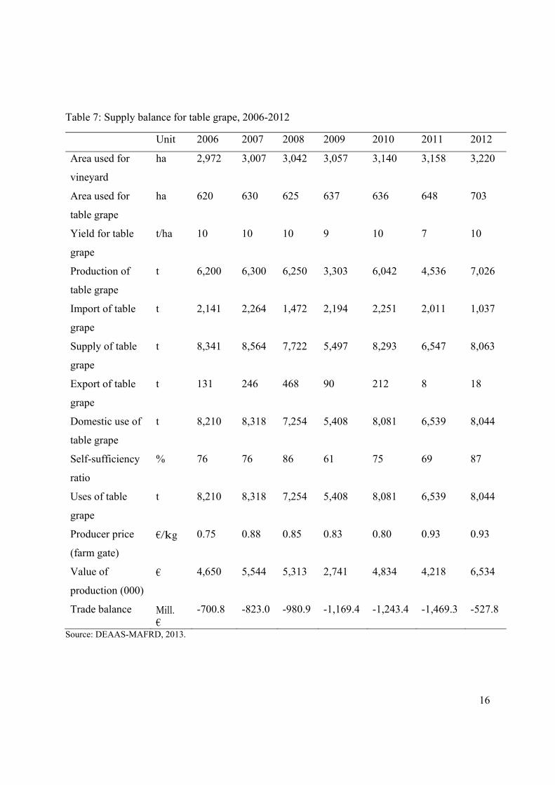
Table 7: Supply balance for table grape, 2006-2012 .................................................................... 16

Table 8: Total area distribution among cultivated wine and table grape varieties ....................... 17

Table 9: Wine production, 2008-2012 ......................................................................................... 18

Table 10: Stock of the selected animals in Kosovo in 000 of units, 2006-2012 ........................... 19

Table 11: Main agri-food import/export commodity by group in 2012 ....................................... 24

Table 12: Selected measures to be implemented in Kosovo for the period of time 2014-2020 ... 31

Table 13: Kosovo's MAFRD budget in million EUR, 2008-2012 ............................................... 32

Table 14: List of frequently cited positive and negative externalities provided by agriculture ... 55

Table 15: Distribution of Kosovo’s total area and agricultural used area by soil types ............... 64

Table 16: Information on the data obtained through the survey and the analysis performed ....... 67

Table 17: Parameters related to farm soil quality ......................................................................... 73

Table 18: Data and analysis performed to describe soil quality at farm level .............................. 73

Table 19: Data and analysis performed to assess agri-biodiversity provided by farms ................ 74

Table 20: Summary statistics of the farm household characteristics ............................................ 75

Table 21: Summary statistics of employment status of the family farms ..................................... 76

Table 22: Correlation of the farm household income sources with farm characteristics .............. 78

Table 23: Annual income of farm households by source of income ............................................ 79

Table 24: Distribution of the farms by farming experience .......................................................... 80

Table 25: Selected chemical soil quality indicators and scoring functions .................................. 85

Table 26: Pattern matrix of soil chemical parameters in cultivated land at tomato farms ............ 86

Table 27: Correlation matrix of the soil chemical parameters in cultivated land at tomato farms 87

Table 28: Calculation of the soil quality index at tomato farms ................................................... 88

Table 29: Soil quality index values and soil parameter threshold values and interpretations ...... 90

Table 30: The SQII and SQIO of tomato farms using normative approach ................................. 91

Table 31: The SQII and SQIO of grape farms using a normative approach ................................. 92

Table 32: The SQII and SQIO of apple farms using principle component analysis and a

normative approach ....................................................................................................................... 93

Table 33: Descriptive statistics of the input and output variables for TE estimation of tomato

farms ........................................................................................................................................... 110

Table 34: Average input oriented technical efficiency scores for tomato farms ........................ 110

Table 35: Bias-corrected efficiency scores for tomato farms under VRS assumption ............... 111

Table 36: Descriptive statistics of the input slacks for tomato farms ......................................... 112

Table 37: Bias-corrected efficiency scores for tomato farms under VRS assumption ............... 113

Table 38: Descriptive statistics of the inputs and output used for TE estimation of the grape

farms ........................................................................................................................................... 113

Table 39: Bias-corrected efficiency scores for grape farms under VRS assumption ................. 114

Table 40: Bias-corrected efficiency scores for grape farms under VRS assumption ................. 115

Table 41: Descriptive statistics of the inputs and output used for TE estimation of the apple farms

..................................................................................................................................................... 115

Table 42: Bias-corrected efficiency scores for apple farms under VRS assumption ................. 116

Table 43: Descriptive statistics of the input slacks at apple farms ............................................. 117

Table 44: Bias-corrected efficiency scores for apple farms under VRS assumption ................. 117

Table 45: Descriptive statistics of the input and output variables for CE and RE estimation of

tomato farms ............................................................................................................................... 118

Table 46: Descriptive statistics of the cost efficiency scores of tomato farms ........................... 118

Table 47: Descriptive statistics of allocative (input-mix) efficiency scores of tomato farms .... 119

Table 48: Distribution of the input-oriented efficiency scores of tomato farms ......................... 119

Table 49: Descriptive statistics of the revenue efficiency scores of tomato farms ..................... 120

Table 50: Distribution of the output-oriented efficiency scores of tomato farms ....................... 121

Table 51: Descriptive statistics of the input and output variables for CE and RE estimation of

grape farms .................................................................................................................................. 122

Table 52: Descriptive statistics of the cost efficiency scores of grape farms ............................. 122

Table 53: Descriptive statistics of allocative (input-mix) efficiency scores of grape farms ...... 122

Table 54: Distribution of the input-oriented efficiency scores of grape farms ........................... 123

Table 55: Descriptive statistics of the revenue efficiency scores of grape farms ....................... 124

Table 56: Distribution of the output-oriented efficiency scores of grape farms ......................... 124

Table 57: Descriptive statistics of the input and output variables costs of apple farms ............. 125

Table 58: Distribution of the input-oriented efficiency scores of apple farms ........................... 126

Table 59: Regression results of the efficiency scores and other tomato farm characteristics .... 129

Table 60: Regression results of the TE, CAE and SE scores and other grape farm characteristics

..................................................................................................................................................... 131

Table 61: Regression results of the efficiency scores and other apple farm characteristics ....... 134

Table 62: Descriptive statistics of the environmental variables included in efficiency measure of

tomato farms ............................................................................................................................... 137

Table 63: Descriptive statistics of the output-oriented ETE score of tomato farms ................... 137

Table 64: Bias-corrected ETE scores for tomato farms under VRS assumption ........................ 137

Table 65: Distribution of the output-oriented efficiency scores of tomato farms ....................... 138

Table 66: The group of tomato farms increased in ranking at ETE ............................................ 139

Table 67: The group of tomato farms with no difference in ranking at ETE ............................. 140

Table 68: The group of tomato farms which decreased in ranking at ETE ................................ 141

Table 69: Descriptive statistics of the environmental variables included in efficiency measure at

grape farms .................................................................................................................................. 142

Table 70: Bias-corrected ETE scores of grape farms under VRS assumption ........................... 143

Table 71: Distribution of the output-oriented efficiency scores of grape farms ......................... 143

Table 72: The group of grape farms increased in ranking at ETE .............................................. 144

Table 73: The group of grape farms with no difference in ranking at ETE ................................ 145

Table 74: The group of grape farms decreased in ranking at ETE ............................................. 146

Table 75: Descriptive statistics of the environmental variables included in the efficiency measure

of apple farms ............................................................................................................................. 147

Table 76: Bias-corrected ETE scores of apple farms under VRS assumption ........................... 147

Table 77: Distribution of the output-oriented efficiency scores of apple farms ......................... 148

Table 78: The group of apple farms increased in ranking at ETE .............................................. 149

Table 79: The group of apple farms with no difference in ranking at ETE ................................ 150

Table 80: The group of apple farms decreased in ranking at ETE ............................................. 151

List of Figures Figure 1: Indices of agricultural goods output 2005-2011 ............................................................ 10

Figure 2: Yield indices of the selected crops in the study, 2007-2013 ......................................... 13

Figure 3: Grape yields comparisons in t/ha with the EU and WBs, 2010-2012 ........................... 15

Figure 4: Stock indices of the selected animals in Kosovo, 2006-2012 ....................................... 20

Figure 5: Agricultural output price indices in Kosovo, 2005-2012 .............................................. 21

Figure 6: Agricultural input price indices in Kosovo, 2005-2012 ................................................ 22

Figure 7: Annual trade balance in food and agricultural products in Kosovo, 2005-2012, Mill.

EUR............................................................................................................................................... 23

Figure 8: Agro-food exports to EU, WBs and other countries in %, 2012 ................................... 24

Figure 9: Agro-food imports to EU, WBs and other countries in %, 2012 .................................. 24

Figure 10: Operational structure of the MAFRD .......................................................................... 28

Figure 11: Budgetary expenditure for agri-food sector in rural areas (million EUR) .................. 32

Figure 12: Structure of the direct payments based on area/animal 2008-2012, Kosovo .............. 33

Figure 13: Budgetary expenditure for rural development measures (million EUR) .................... 34

Figure 14: Budgetary expenditure for competitiveness (million EUR) ........................................ 35

Figure 15: Framework for performance assessment ..................................................................... 41

Figure 16: Production frontier of the single input and single output under CRS and VRS

assumption for the DMUs A, B, C, and D .................................................................................... 46

Figure 17: Technical efficiency .................................................................................................... 47

Figure 18: Pure technical and scale efficiency ............................................................................. 48

Figure 19: Classification of external effects ................................................................................. 52

Figure 20: Negative externality in a single commodity market .................................................... 53

Figure 21: Positive externality in a single commodity market ..................................................... 53

Figure 22: Typology of the total economic value approach ......................................................... 56

Figure 23: Pedological map of Kosovo ........................................................................................ 65

Figure 24: Location of the sampled tomato farms ........................................................................ 69

Figure 25: Location of the sampled apple farms .......................................................................... 70

Figure 26: Location of the sampled grape farms .......................................................................... 71

Figure 27: Scheme of the soil sampling ........................................................................................ 71

Figure 28: Distribution of the total soil samples among farms in cultivated and uncultivated land

....................................................................................................................................................... 72

Figure 29: Satisfied level of farmers in farming activities ........................................................... 81

Figure 30: A generalized framework for developing soil quality indices (from Karlen et al. 2001)

....................................................................................................................................................... 84

Figure 31: PCA scree plot of soil chemical parameters in cultivated land at tomato farms ......... 86

Figure 32: Comparison of the estimated SQI for cultivated and uncultivated land of tomato farms

using a normative approach .......................................................................................................... 91

Figure 33: Comparison of the estimated SQI for cultivated and uncultivated land of grape farms


Figure 34: Comparison of the estimated SQI for cultivated and uncultivated land of apple farms


Figure 35: SHDI graphical summary of tomato producers ......................................................... 100

Figure 36: SHDI graphical summary of grape producers ........................................................... 100

Figure 37: SHDI graphical summary of apple producers ........................................................... 101

Figure 38: Box-plot of SHDI of tomato, grape and apple farms ............................................... 102

Figure 39: Scatter-plot of the CAE scores and inputs used by tomato farms ............................. 120

Figure 40: Scatter-plot of the CAEInput-Mix scores and inputs used by grape farms .................... 123

Figure 41: Scatter-plot of the CAE scores and inputs used by apple farms ............................... 126

ABBREVIATIONS

AE Allocative Efficiency

ANOVA Analysis of Variance

ARDP Agriculture and Rural Development Program

BCC Banker, Charnes, and Cooper

CAE Cost Allocative Efficiency

CAP Common Agricultural Policy

CCR Charnes, Cooper and Rhodes

CE Cost Efficiency

CEFTA Central European Free Trade Agreement

CI Confidence Interval

CRS Constant Returns to Scale

DEA Data Envelopment Analysis

DMU Decision Making Unit

DRS Decreasing Returns to Scale

EAP Environmental Action Plan

ETE Environmental Efficiency

EU European Union

EUR Euro

FADN Farm Accounting Data Network

FAO Food and Agriculture Organization

FYROM Former Yugoslav Republic of Macedonia

GDP Gross Domestic Product

GVA Gross Value Added

HACCP Hazard Analysis and Critical Control Points

HH Household

HNV High Nature Value

IPA II Instrument for Pre-accession Assistance II

IPARD Instrument for Pre-Accession Assistance for Rural Development

IRS Increasing Return to Scale

LAG Local Action Groups

LFA Less Favored Areas

LP Linear Programming

LSF Linear Scoring Function

LS Linear Score

MAFRD Ministry of Agriculture Forestry and Rural Development

MA Managing Authority

MAO Municipal Agricultural Office

MC Monitoring Committee

MTE Mid-Term Evaluation

NA Normative Approach

NIRS Non Increasing Return to Scale

NSQI Normalized Soil Quality Index

NVA Net Value Added

PCA Principle Component Analysis

PD Paying Department

PIMDEA Performance Improvement Management Software

PTE Pure Technical Efficiency

PU Paying Unit

RAE Revenue Allocative Efficiency

RE Revenue Efficiency

SBM Slacks Based Measure

SD Standard Deviation

SE Scale Efficiency

SHDI Shannon's Diversity Index

SPSS Statistical Package of the Social Sciences

SQII Soil Quality Index in Cultivated Land

SQIO Soil Quality Index in Uncultivated Land

SQI Soil Quality Index

TE Technical Efficiency

UAA Utilized Agricultural Area

VA Value Added

VL Value Lost

VRS Variable Returns to Scale

WB Western Balkans

1

1. INTRODUCTION

Agriculture plays a multifunctional role by producing food and fiber which already have visible

values in the market (market prices). In addition, it also produces other goods and services that

do not have market prices and in general are not valued. Therefore, the system of completely free

market was not shown to be a perfect way of solving all economic problems and interventions to

modify the outcomes to '[correct] for market failure' became a necessity for achieving better

results for the welfare of society as a whole (Mankiw, N. G., 2007). The market mechanism does

not function for the provision of goods with a high degree of publicness (Cooper T., 2009). It

does not take into account externalities as one of the main deficiencies along with others like

imperfect knowledge, imperfect competition, friction in the market mechanism and failure to

reflect non-economic goals (Just R., 2004). The environmental externalities on which

interventions are based on are the outputs from production that can be either negative or positive.

Such outputs are usually disregarded by producers in their decision making process, as they

consider only private costs and benefits. Many of these non-marketable positive and negative

outputs are closely linked to the agriculture and forestry production. Whenever such positive

outputs occur, intervention to encourage these kinds of activities and production of more of these

products through support given to the farmers can be justified, as their role is not found only in

securing food supply but also in improving environmental quality. However, there are also

negative outputs ensuing from the agriculture and forestry production which are carrying costs

for the society which needs to be identified and corrected by intervention.

The debates and reforms on optimization of policies and instruments of the Common

Agricultural Policy (CAP) are reflecting/reflect the change of societal demand and political

priorities and have been taking place since the early 1990s. The Single European Act (1986) was

the major revision of the Treaty of Rome (1957), considering environmental protection in all

new Community legislation. The Treaties of Maastricht (1992) and Amsterdam (1997) made

sustainable development a core of European Union (EU) objective and the Agenda 2000

agreement included a revised set of objectives of the CAP that included 'integration of

environmental goals into the CAP' and the 'promotion of sustainable agriculture' (Hill B. , 2012).

2

A considerable share of the CAP's budget in Pillar two (rural development) goes to agri-

environment related schemes such as payments to farmers in Less Favored Areas (LFA),

conversion to organic production, and a relatively smaller amount to socio-economic purposes.

Up until now, a lot of criticism from different researchers was raised and addressed to the CAP

regarding inconsistencies between objectives and the policy measures implemented (Arovuori,

2008).

The Food and Agriculture Organization (FAO) concept note on the remuneration of positive

externalities in the agriculture and food sector is part of an effort to link CAP agri-environmental

policies to other payments for environmental services (FAO, 2010). The nature and reversal of

biodiversity decline is one of the four priorities identified in the Environmental Action Plan

(EAP) 2002-2012. The emphasis of action plan and policy primarily lays on confining

agricultural practices that pose threats to species and their habitats and encourage new practices

that bring benefits to them. Farmland biodiversity is considered to be a public good which has an

intrinsic value (Cooper T., 2009). The intensity level of agricultural production determines

enhancement of species richness and in this regard extensive agricultural practices is often

considered to be a good way of creating an optimal level of disturbances for generating multiple

ecological niches that support a wider range of species (Kleijn, 2008). Regardless if farmland

biodiversity is seen as being comprised of species and habitats or as a range of related services

that they provide to society, both definitions share the characteristics of public goods (Fisher B.,

and Turner R. K., 2008).

It is understood that market prices may serve as a poor proxy for individual or societal values

and that ecosystem service assessment need to include spatial and temporal aspects to be truly

policy relevant (Fisher B., 2011). Incorporating ecosystem services into land use decisions

typically favors conservation activities or sustainable management over the conversion of intact

ecosystems (Balmford A., 2002). Farm characteristics such as crop cover, varieties of crop, land

use, practices applied in input use, machinery, and size of the fields are considered to be the main

determinants of level at which agriculture can contribute to the provision of public goods e.g.

land fragmentation, land ownership and crop diversity (Manjunathaa A.V., 2012).

3

It is well known that most of the crops in horticultural production system are intensively

cultivated with significant use of fertilizers, pesticides and herbicides. On the one side, the

cultivation of horticultural crops on open fields can provide color and veriety for the landscape,

but as an intensive production system the provision of environmental public goods can increase

through adoption of organic methods, biological pest control, and good practices of soil

management that avoid soil erosion and contamination (Cooper T., 2009). Permanent crops like

grape and apple orchards provide an important habitat for many species including mammals,

birds, insects and plants. The number of cultivated grape and apple varieties is important

compound of biodiversity.

In addition to the private land owner's interest to manage the soil resource in a sustainable way

(e.g. through careful application of the fertilizers, pesticides, herbicides and machinery), society

also has interest in maintaining good soil functionality at the present time and for the future

generations, as it is seen not only as a base for food production but also to underpin the provision

of public goods (Cooper T., 2009). The contribution to soil functionality varies among soil

management techniques. Land cover with permanent trees and vegetation, not only contributed

positively to promoting biodiversity interest and soil function but also to the cultural landscapes

(Chen Q., 2014).

Agriculture plays an important role in provisioning of agricultural landscapes, farmland

biodiversity, and water and soil quality which are highly valued by society (Cooper T., 2009).

The absence of economic values for such environmental goods and services generally leads to

degradation of these goods (Kortelainen M., and Kuosmanen T., 2004). Even though there are

evidences for soil quality improvements in the EU countries from agricultural activities, the

situation is still unsatisfactory and there is still possibility for further progress (Cooper T., 2009).

In practice, the provision of biodiversity is not explicitly recognized as a positive output when

production efficiency is measured (Sipiläinen T., Marklund P., Huhtala A., 2008). Therefore,

efficiency measures based only on traditional marketable inputs and outputs without

incorporation of other non-marketable inputs or outputs yields biased efficiency scores.

4

1.1 Problem statement and justification

Despite of its comparative production advantage, due to the damages caused by the last war

(1999), in the last two decades Kosovo became a net importer for most of the agricultural

products, including horticultural products (Fischer Ch., 2004). Horticulture production is of high

importance for the agriculture sector, accounting for approximately 40% of the agricultural

output (Imami D., 2016). In the last decade, the demand for horticultural products increased

more than for any other agricultural product (MAFRD, 2014) and it is expected to further rise in

the future, driven by the augment in purchasing power (Imami D., 2016). According to the Green

Report 2014 published by the MAFRD, the self-sufficiency ratio for most of the horticultural

products (with exception of potatoes) is relatively low. The increase of the self-sufficiency ratio

for tomatoes was fairly low during the time period 2007-2013 (2007 - 49.9%; 2013 - 55.7%)

compared to the one for apples, which was significantly higher (2007 – 38.9%; 56.7%)

(MAFRD, 2014).

Since 2007 there has been a significant improvement of financial support from the Government

of Kosovo and the international donor community for the agriculture sector. In the last few years

the private side has shown a remarkable interest to invest in the agrifood sector. One of the main

objectives of the agriculture sector stated in the Kosovo Agriculture and Rural Development Plan

(ARDP) 2007-2013 as well as in the ARDP 2014-2020 is to increase competitiveness and the

efficiency of primary agricultural production which will yield higher income for the farmers and

improve living standards in rural areas, as well as impact import substitution and take advantage

of export markets.

Taking into account the stated objectives in the ARDP 2007-2013 and 2014-2020, we considered

that measuring the efficiency of farms is crucial in order to improve understanding of factors that

explain differences in the efficiency among farms and also provides possibilities for better

utilization of resources (land, labor and capital) by farms. Despite its importance until 2014 there

were no studies conducted on measuring neither farm efficiency, productivity growth nor

changes in the agriculture sector of Kosovo. A first study entitled ‘Migration and agriculture

efficiency-evidence from Kosovo’ was published in 2014 by Sauer J. et al.. The study used a

5

parametric stochastic frontier approach to estimate efficiency of the farms in Kosovo. The mean

of the technical efficiency for the whole sample was estimated to be 61.1% (SD = 24.3%) (Sauer

J., Gorton M., Davidova S., 2014). The data used in this study was coming from Annual

Agricultural Household Surveys conducted by Statistical Office of Kosovo 2005-2008. It should

be emphasized that agricultural households included in the sample were subsistence household

farms that cultivated more than 0.10 hectares (ha) of arable land or less than 0.10 ha of utilized

arable land but had at least: 1 cow or 5 sheep/goats or 3 pigs or 50 poultry or 20 beehives. Just

recently a new study was published by (Vuçitërna R., 2017) on ‘Efficiency and Competitiveness

of Kosovo Raspberry Producers’. The study used an input-oriented DEA method to measure

technical efficiency of the raspberry producers in Kosovo. Nevertheless the attention and support

given to the agriculture sector by the government and other international donor organizations has

increased significantly in recent years and is expected to further increase in the coming years

(Imami D., 2016).

Considering all these factors/circumstances, such as the objectives of the agriculture sector in

Kosovo, the low self-sufficiency ratio, the negative trade balance, the increased financial support

given to the agriculture sector, the importance of efficiency measurements and analysis in regard

to the agriculture sector’s objectives, the absence of studies on the efficiency, and the need for

more efficient use of existing technologies and resources. All these factors justify the need to

conduct a study on this topic.

1.2 Objective of the study

The overall objective of the study was to estimate efficiency levels among the private farms in

Kosovo which were oriented more on tomato, grape and apple production. The utilized

agricutlural area for vegetables and fruits was used as criterion in the selection process of crops

to be included in the study. Taking into consideration this criterion tomatoes (within vegetables),

apples and grapes (within fruits) were the most cultivated crops.

Within this context the study aimed to achieve the following specific objectives:

6

• Estimate economic efficiency of the three different production systems considered

in the study;

• Estimate environmental efficiency of three different production systems with the

inclusion of environmental variables into efficiency measure;

• Identify factors that comprehensively/extensively explain the variation of the

efficiency scores among the selected farms for each production system and

estimate potential reduction of the input costs or increase of output levels that can

improve economic and environmental efficiency of the farms.

• Derive recommendations for more efficient use of existing technology and

resources and foster the degree of multifunctionality.

7

2. OVERVIEW OF THE AGRICULTURE SECTOR IN KOSOVO

2.1Backgroundinformation

In 2012, the real Gross Domestic Product (GDP) growth was 2.5% and GDP per capita 2,721.0

EUR. Compared to 2011, an inflation rate in 2012 was lower for 2.5%. Even though

unemployment rate shows a decrease in 2013, it still remains a serious problem for the country’s

economy and at a very high rate in comparison to the other regional countries and with the EU

countries. The unemployment rate in 2013 was estimated to be 30.0 %. The share of food,

beverages and tobacco in total household’s expenditures in 2012 was at 45%.

Table 1: Macroeconomic indicators

Indicator Unit 2006 2007 2008 2009 2010 2011 2012

Total area km2 10,908 10,908 10,908 10,908 10,908 10,908 10,908

Population 000 2,100 2,130 2,153 2,181 2,181 1,740 1,816

GDP

(at current prices)

mill.

EUR 3,120 3,461 3,940 4,008 4,291 4,770 4,916

Value added

(at current prices)

mill.

EUR 2,745 3,034 3,487 3,533 3,697 4,043 :

Economic growth

(real change in

GDP) %

3.4 8.3 7.2 3.5 3.2

4.4 2.5

GDP per capita EUR 1,890 2,062 2,310 2,311 2,436 2,668 2,721

Inflation % 0.6 4.4 9.4 -2.4 3.5 7.3 2.5

Unemployment rate % 44.9 43.6 47.5 45.4 44.0 44.8 30.9

Source: Kosovo Agency of Statistics, 2006-2012.

8

2.2 The role of the agriculture sector in the country’s economy

Agriculture has historically been an important sector for the economy of Kosovo. The average

share of the agriculture, forestry, hunting and fishery sector in Gross Value Added (GVA) for the

period of time 2006-2011 was about 15%. The agriculture share in total employment rate in 2012

was estimated to be 4.6% (Table 2). When we consider the contribution of the agriculture sector

in GVA and the estimated employment rate into agriculture, it gives an indication of a sector

with good efficiency rate. However, this figure (4.6%) covers only formal employment in the

agriculture sector. The Agriculture sector in Kosovo aside from the employment and its

economic contribution it also provides a social safety net for a large number of the family farms

living in rural areas. Agriculture is at a small scale, predominating subsistence farms with small

land tenure and enormously fragmented (MAFRD, 2013).

Table 2: Key agricultural statistics

Unit 2006 2007 2008 2009 2010 2011 2012

GVA of the agriculture, forestry, hunting and fishery sector GVA (at current prices)

Mill. EUR 372.4 479.6 526.3 532.7 630.3 705.5 615

Share in GVA of all activities % 13.6 15.8 15.1 15.1 17.1 17.5 :

Employment in the agriculture, forestry, hunting and fishery sector

Number 000 : : : : : : 13900.

0Share in total employment % : : : : : : 4.6 Trade in food and agricultural products Export of agri-food products

Mill. EUR 9.9 17.0 18.15 17.4 24.7 26.2 20.6

Share in export of all products % 8.9 10.3 9.1 10.5 8.3 8.2 7.5Import of agri-food products

Mill. EUR 319.0 384.1 432.3 431.1 482.8 561.4 572.7

Share in import of all products % 24.4 24.4 22.4 22.3 22.4 22.5 22.8Trade balance in agri-food products

Mill. EUR -309.1 -367.1 -414.2 -413.7 -458.1 -535.2 -552.1

Source: Kosovo Agency of Statistics, 2006-2012; Green Report Kosovo 2013.

9

2.3 Land resource and farm structure

According to the latest statistics, the total agricultural land of Kosovo amounts at 357,748 ha, out

of which 253,563 ha is arable land, 7,071 ha land under permanent crops (orchards and

vineyards), and 97,114 ha land under permanent grassland (meadows and pastures). The total

farm land is used by 185,765 farms, out of which 185,424 (99%) are small farms (MAFRD,

2013). The share of the utilized agricultural area from total area is 25.4% and the utilized

agricultural area per 1,000 of population is 125.6 ha.

Kosovo has an unfavorable farm structure (Table 3), with an average Utilized Agricultural Area

(UAA) per holding of 1.5 ha, fragmented into 7 plots. For the period of time 2007-2012 the

number of farms remained almost constant but the UAA per holding increased by 5.7% and this

was notably taking place at large and specialized farms (MAFRD, 2013).

Table 3: Farm structure by size in 2012

Farm size (ha) Number of

farms

Area (ha) % of farms

0.01 – 0.5 45,818 13,300 24.7

0.51 – 1.0 51,665 39,385 27.8

1.01 - 1.5 35,589 43,772 19.2

1.51 - 2.0 15,719 27,830 8.5

2.01 – 3.0 19,995 49,340 10.8

3.01 – 4.0 5,777 20,009 3.1

4.01 – 5.0 3,748 16,646 2.0

5.01 – 6.0 2,317 12,622 1.2

6.01 – 8.0 2,582 17,847 1.4

8.01 – 10 1,007 8,972 0.5

> 10 1,547 27,641 0.8

Total 185,765 277,364 100.0

Source: Green Report Kosovo 2013, 2013.

10

2.4 Agricultural production and consumption

The agricultural production is characterized with a small farm size, outdated technology and

farming practices, inefficient management practices, inappropriate use of the agricultural inputs,

an unfavorable credit market and an insufficient provision of technical expertise. All these

highlighted factors bring Kosovo’s agricultural production/yields fairly below the EU averages.

The majority of the agricultural production is sold at the domestic market for human

consumption and limited amount to the processing industry, mainly without a long term

contractual bases. Due to the many small farms and the limited amount of the agricultural

production, Kosovo’s agricultural processors are facing high collection costs and consequently

making them less competitive in the market.

The average share of the crops in total agricultural goods output for the period of tie 2010-2012,

was considerably higher (54.3%) compared to the livestock output (45.7%). However, the

contribution of the livestock branch to the total agricultural goods output was apparently more

constant for the given period of time (Figure 1).

Figure 1: Indices of agricultural goods output 2005-2011

0

20

40

60

80

100

120

140

2005 2006 2007 2008 2009 2010 2011

Index (2005=100)

Total Agricultural Goods Output ‐ Crops ‐ Livestock

11

The most important crops for agricultural production are cereals, predominantly wheat and

maize. In 2012, the total cultivated area with cereals was 137,214 ha, out of which 31,181 ha was

cultivated with maize and 3,115 ha with rye, barley, malting barley and oat (Table 4). A high

proportion of the agriculture area is cultivated with forage crops such as hay, grass, alfalfa,

trefoil, vetch, wheat fodder, rye fodder, barley fodder, oat fodder, maize fodder and in total these

crops sum up to 94,400 ha.

Table 4: Crop production structure 2006-2012, in 000 ha

Crop 2006 2007 2008 2009 2010 2011 2012

Cereals 110.0 102.4 115.0 120.0 119.9 121.1 137.2

Potato 3.1 5.0 3.7 3.4 3.8 3.7 3.2

Grapes 3.0 3.0 3.0 3.1 3.1 3.2 3.2

Fruits 3.2 3.8 4.0 3.0 3.4 3.6 3.9

Vegetable 8.1 8.3 8.6 8.4 9.0 9.2 8.4

Beans 4.8 4.4 4.2 4.1 3.6 3.3 3.0

Forage 96.7 108.4 104.7 91.4 99 98.8 94.4


A considerable area of the agricultural land is occupied with vegetable production (8,405 ha,

2012; Table 5). The most cultivated and consumed vegetables in Kosovo are tomato, pepper,

cucumber, water melon, pumpkin, cabbage, and onion. In 2012, among the all cultivated

vegetables the highest increase of the cultivated area was recorded for tomato (31%) and the

production rose by 22%.

12

Table 5: Area and production of the main cultivated vegetables, 2006-2012

Cultivated area Unit 2006 2007 2008 2009 2010 2011 2012

Area used for vegetable ha 8111 8312 8592 8351 8987 9190 8405

Area used for tomato ha 787 923 903 821 935 967 1271

Tomato production t 15195 14697 20587 15107 60318 62358 13693

Share of tomato % 9.70 11.10 10.50 9.83 10.40 10.52 15.12

Yield t/ha 19.30 15.92 22.79 18.40 64.51 64.48 10.77

Area used for pepper ha 2733 2231 2523 2955 2914 2993 3153

Share of pepper % 33.69 26.84 29.36 35.38 32.42 32.56 37.51

Pepper production t 62925 35959 51274 46669 93924 96322 50744

Yield t/ha 23.02 16.11 20.32 15.79 32.23 32.18 16.09

Area used for cucumber ha 277 344 278 316 343 359 255

Share of cucumber % 3.41 4.13 3.23 3.78 3.81 3.90 3.03

Production of cucumber t 7528 7088 9032 7199 12902 13502 5239

Yield t/ha 27.17 20.60 32.48 22.78 37.61 37.61 20.54

Area used for water melon ha 700 901 1029 954 1141 1240 847

Share of water melon % 8.63 10.83 11.97 11.42 12.69 13.49 10.07

Production of water melon t 18821 15048 24736 18896 25743 27975 17080

Yield t/ha 26.88 16.70 24.03 19.80 22.56 22.56 20.16

Area used for cabbage ha 921 620 703 962 836 842 568

Share of cabbage % 11.35 7.45 8.18 11.51 9.30 9.16 6.75

Production of cabbage t 25012 15425 19041 27895 22988 23154 13975

Yield t/ha 27.15 24.87 27.08 28.99 27.49 27.49 24.60

Area used for onion ha 810 1059 1205 798 1043 1074 881

Share of onion % 9.98 12.74 14.02 9.55 11.60 11.68 10.48

Production of onion t 11376 10934 15987 8697 13257 13655 8601

Yield t/ha 14.04 10.32 13.26 10.89 12.71 12.71 9.76

Other % 23.21 26.87 22.70 18.50 19.75 18.66 17.01

Total cultivated area % 100 100 100 100 100 100 100

Source: Kosovo Agency of Statistics: Agricultural Households Survey, 2006-2012.

13

Increasing productivity and competitiveness of the agricultural production is a long term policy

objective in Kosovo. However, the average yields for crops (t/ha) still remain below the

European average. The average yield in wheat production for the period of time 2010-2012 was

73.3% of the EU-27 average. In 2012, the average maize yield was recorded at 2.8 t/ha which is

still fairly low compared to the EU-27. In 2012, the average yield for potatoes was 55% lower

compared to the years 2011 and 2010 (Figure 2). The average yield for potatoes from 2010-2012

was recorded at 19 t/ha, which is 69% of the average yields realized by EU farmers.

Figure 2: Yield indices of the selected crops in the study, 2007-2013

Source: Green Report 2014, MAFRD.

In 2012, the total area with the fruit production was 7,071 ha and the most cultivated fruits were

apple, pear, plum, sour cherry, and grape which all together take up to 95% of the cultivated area

with fruits. About 25% of the total cultivated area with fruits is planted with apple and compared

with the previous year this area in 2012 decreased by 4%. The range of the planted apple

cultivars is wide up to 20 but those most frequently grown are Idared, Golden Delicious,

Jonagold, Granny Smith and the rootstocks used are mainly M9, MM106, and M26

(Spornberger, et al., 2014). The total domestic production of the apple fruit fulfilled only 53% of

the domestic needs (Table 6) and out of the total domestic production around 60% is used for the

household needs (MAFRD, 2013).

0

50

100

150

200

250

300

350

400

450

2007 2008 2009 2010 2011 2012 2013

Tomato Apple Grape

14

Table 6: Supply balance for apple, 2006-2012

Unit 2006 2007 2008 2009 2010 2011 2012

Area used for fruits ha 6,157 6,812 6,999 6,027 6,578 6,733 7,071

Area used for apple ha 1,096 1,068 1,686 1,355 1,661 1,790 1,725

Share of apple % 17.8 15.7 24.1 22.5 25.3 26.6 24.4

Yield t/ha 8.55 5.91 7.48 8.67 7.55 7.55 4.71

Production t 9,372 6,307 12,612 11,742 12,545 13,523 8,120

Import of apple t 10,759 9,929 9,684 11,161 12,221 11,084 7,134

Supply t 20,131 16,236 22,296 22,903 24,766 24,607 15,254

Export of apple t 19 3 63 5 7 3 11

Domestic uses t 20,112 16,233 22,234 22,898 24,758 24,604 15,243

Self-sufficiency

ratio

% 46.6 38.9 56.7 51.3 50.7 55.0 53.3

Waste t 937 631 1,261 1,174 1,255 1,352 812

Own final

consumption

t 5,061 3,406 6,810 6,341 6,774 7,302 4,385

Human consumption

total

t 19,175 15,602 20,972 21,724 23,504 23,252 14,431

Domestic uses total t 20,112 16,233 22,234 22,898 24,758 24,604 15,243

Producer price (farm

gate)

€/kg 0.51 0.56 0.60 0.51 0.49 0.49 0.54

Value of production Mill.

EUR

4.3 3.2 6.8 5.4 5.5 6.0 3.9

Trade balance for

apple

Mill.EUR -2.3 -2.4 -2.7 -3.0 -3.4 -3.3 -4.2

Source: MAFRD, 2013.

Grape and wine production in Kosovo has a history of thousands of years. Different topographies

and archeological discoveries give an evidence of ancient Ilirian-Albanian tradition of the grape

and wine production. In the cadastral documents of XI-XV centuries, many villages of the

15

municipality of Vushtrri and the territory of Kosovo as whole, was recognized as grape cultivator

area (Gjonbalaj, et al., 2009).

Yet, the wine sector remains an important and most promising branch of the agriculture sector.

In 2012, the total cultivated area with grape reached at 3,220 ha out of which 22% belong to the

table grape varieties. Grape is the only fruit where Kosovo farmers attained higher average yields

in 2010-2012 (21.5%) compared to the EU farmers (Figure 3). In the last three years, the average

yield for grape was 7.9 t/ha which is 10% higher than in other Western Balkan countries. Kosovo

farmers reached comparable grape yields with Italian and Greek farmers.

Figure 3: Grape yields comparisons in t/ha with the EU and WBs, 2010-2012

Source: FAO/SWG Project.

In comparison to the previous year the total production of the table grape in 2012 increased by

55%. However, the trade balance remains negative with 528 Mill. EUR and the total production

of 7,026 tons cover 87% of the domestic needs (MAFRD, 2013).

0

2

4

6

8

10

12

14

CY BiH SK CZ RO PT BG HU RS FR ES HR AT SI KS MN IT EL DE MK LU

16

Table 7: Supply balance for table grape, 2006-2012

Unit 2006 2007 2008 2009 2010 2011 2012

Area used for

vineyard

ha 2,972 3,007 3,042 3,057 3,140 3,158 3,220

Area used for

table grape

ha 620 630 625 637 636 648 703

Yield for table

grape

t/ha 10 10 10 9 10 7 10

Production of

table grape

t 6,200 6,300 6,250 3,303 6,042 4,536 7,026

Import of table

grape

t 2,141 2,264 1,472 2,194 2,251 2,011 1,037

Supply of table

grape

t 8,341 8,564 7,722 5,497 8,293 6,547 8,063

Export of table

grape

t 131 246 468 90 212 8 18

Domestic use of

table grape

t 8,210 8,318 7,254 5,408 8,081 6,539 8,044

Self-sufficiency

ratio

% 76 76 86 61 75 69 87

Uses of table

grape

t 8,210 8,318 7,254 5,408 8,081 6,539 8,044

Producer price

(farm gate)

€/kg 0.75 0.88 0.85 0.83 0.80 0.93 0.93

Value of

production (000)

€ 4,650 5,544 5,313 2,741 4,834 4,218 6,534

Trade balance Mill. €

-700.8 -823.0 -980.9 -1,169.4 -1,243.4 -1,469.3 -527.8

Source: DEAAS-MAFRD, 2013.

17

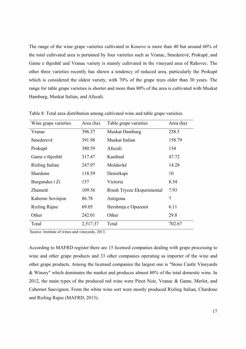
The range of the wine grape varieties cultivated in Kosovo is more than 40 but around 60% of

the total cultivated area is pertained by four varieties such as Vranac, Smederevë, Prokupë, and

Game e thjeshtë and Vranac variety is mainly cultivated in the vineyard area of Rahovec. The

other three varieties recently has shown a tendency of reduced area, particularly the Prokupë

which is considered the oldest variety, with 70% of the grape trees older than 30 years. The

range for table grape varieties is shorter and more than 80% of the area is cultivated with Muskat

Hamburg, Muskat Italian, and Afuzali.

Table 8: Total area distribution among cultivated wine and table grape varieties

Wine grape varieties Area (ha) Table grape varieties Area (ha)

Vranac 396.37 Muskat Hamburg 258.5

Smederevë 391.98 Muskat Italian 158.79

Prokupë 380.59 Afuzali 154

Game e thjeshtë 317.47 Kardinal 47.72

Rizling Italian 247.97 Moldavkë 14.28

Shardone 118.59 Demirkapi 10

Burgundez i Zi 157 Victoria 8.54

Zhametë 109.56 Rrush Tryeze Eksperimental 7.93

Kaberne Sovinjon 86.78 Antigona 7

Rizling Rajne 69.05 Hershmja e Opuzenit 6.11

Other 242.01 Other 29.8

Total 2,517.37 Total 702.67

Source: Institute of wines and vineyards, 2013.

According to MAFRD register there are 15 licensed companies dealing with grape processing to

wine and other grape products and 33 other companies operating as importer of the wine and

other grape products. Among the licensed companies the largest one is "Stone Castle Vineyards

& Winery" which dominates the market and produces almost 80% of the total domestic wine. In

2012, the main types of the produced red wine were Pinot Noir, Vranac & Game, Merlot, and

Cabernet Sauvignon. From the white wine sort were mostly produced Rizling Italian, Chardone

and Rizling Rajne (MAFRD, 2013).

18

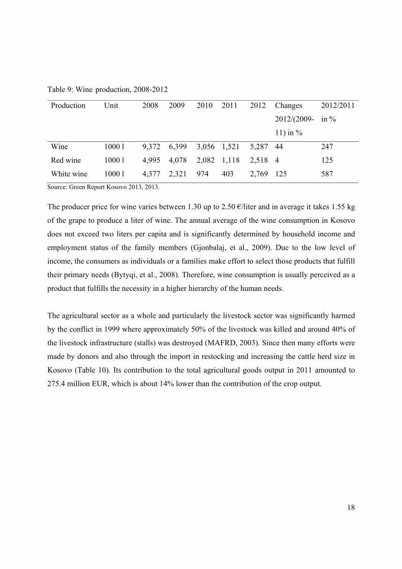
Table 9: Wine production, 2008-2012

Production Unit 2008 2009 2010 2011 2012 Changes

2012/(2009-

11) in %

2012/2011

in %

Wine 1000 l 9,372 6,399 3,056 1,521 5,287 44 247

Red wine 1000 l 4,995 4,078 2,082 1,118 2,518 4 125

White wine 1000 l 4,377 2,321 974 403 2,769 125 587


The producer price for wine varies between 1.30 up to 2.50 €/liter and in average it takes 1.55 kg

of the grape to produce a liter of wine. The annual average of the wine consumption in Kosovo

does not exceed two liters per capita and is significantly determined by household income and

employment status of the family members (Gjonbalaj, et al., 2009). Due to the low level of

income, the consumers as individuals or a families make effort to select those products that fulfill

their primary needs (Bytyqi, et al., 2008). Therefore, wine consumption is usually perceived as a

product that fulfills the necessity in a higher hierarchy of the human needs.

The agricultural sector as a whole and particularly the livestock sector was significantly harmed

by the conflict in 1999 where approximately 50% of the livestock was killed and around 40% of

the livestock infrastructure (stalls) was destroyed (MAFRD, 2003). Since then many efforts were

made by donors and also through the import in restocking and increasing the cattle herd size in

Kosovo (Table 10). Its contribution to the total agricultural goods output in 2011 amounted to

275.4 million EUR, which is about 14% lower than the contribution of the crop output.

19

Table 10: Stock of the selected animals in Kosovo in 000 of units, 2006-2012

Animal 2006 2007 2008 2009 2010 2011 2012

Cattle 381.9 321.6 341.6 344 356.7 361.8 329.21

of which milk

cows 205.38 189.70 191.5 190.2 194.9 196.1 183.34

Pigs 68.223 39.591 26.7 50.58 50.58 50.58 55.7

of which

breeding sows 18 10.4 7.3 12.2 12.2 12.2 :

Sheep/Goats 112.94 151.81 180.12 217.16 229.157 231.209 247.90

of which

breeding

ewes/goats 74.87 108.18 124.12 158.12 163.49 163.49 175.29

Horses 6663 6147 4973 4213 4213 4213 2139

Poultry 2,525 2,278 2,213 2,390 2,347 2,347 2,318

Beehives 72.16 60.95 43.29 43.15 46.95 44.63 46.48

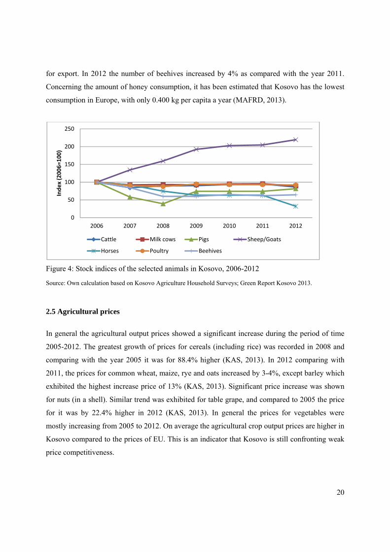
Source: Green Report Kosovo 2013, 2013. Out of the total number of cattle in 2012, dairy caws represent 55.6% and comparing with the

year 2011 the number of dairy caws in stock decreased by 6.5%.The number of total pigs and

breeding sows was increased by 10.1% in 2012 compared to the previous year. Compared to the

other selected animals, the total number of sheep and goats stock showed a significant increase

between 2006 and 2012. In 2006, Kosovo counted 112,943 sheep and goats and compared to the

stock counted in 2012 this number is doubled. In 2012, the number of sheep and goats increased

by 7.3% as compared to the previous year. Negative trend was shown in terms of the total

number of horses in stock for the period of time 2006-2012. In comparison with the last three

previous years, in 2012 the total number of horses in stock decreased by 51%.

The poultry production in Kosovo is characterized by small and medium–scale production units,

mainly oriented on eggs production for consumption, whereas, the production of chicken for

meat is in the consolidation stage. It has been estimated that the production of eggs fulfills the

needs of local costumers by 70% (MAFRD, 2013). Considering suitable environmental

conditions, honey and other beekeeping products were considered products with good potential

20

for export. In 2012 the number of beehives increased by 4% as compared with the year 2011.

Concerning the amount of honey consumption, it has been estimated that Kosovo has the lowest

consumption in Europe, with only 0.400 kg per capita a year (MAFRD, 2013).

Figure 4: Stock indices of the selected animals in Kosovo, 2006-2012

Source: Own calculation based on Kosovo Agriculture Household Surveys; Green Report Kosovo 2013.

2.5 Agricultural prices

In general the agricultural output prices showed a significant increase during the period of time

2005-2012. The greatest growth of prices for cereals (including rice) was recorded in 2008 and

comparing with the year 2005 it was for 88.4% higher (KAS, 2013). In 2012 comparing with

2011, the prices for common wheat, maize, rye and oats increased by 3-4%, except barley which

exhibited the highest increase price of 13% (KAS, 2013). Significant price increase was shown

for nuts (in a shell). Similar trend was exhibited for table grape, and compared to 2005 the price

for it was by 22.4% higher in 2012 (KAS, 2013). In general the prices for vegetables were

mostly increasing from 2005 to 2012. On average the agricultural crop output prices are higher in

Kosovo compared to the prices of EU. This is an indicator that Kosovo is still confronting weak

price competitiveness.

0

50

100

150

200

250

2006 2007 2008 2009 2010 2011 2012

Index (2006=100)

Cattle Milk cows Pigs Sheep/Goats

Horses Poultry Beehives

21

Compared to the crop products, the prices for livestock products were significantly increasing

faster for the given time 2005-2012 (Figure 5). If we compare the price of young cattle in 2005

with the price in 2012, it has increased by 31.8%. Between 2005 and 2012, approximately

similar price increases have occurred to the other livestock products such as pigs (36.1%), lams

(28.6%) and chicken (33.3%). Compared to these livestock products, the prices for eggs and milk

showed smaller increase between 2005 and 2012, 24.9% for eggs and 14.3% for cow’s milk.

The data on total agricultural input prices indicates a continuously increase of prices during the

period of time 2005-2012 (Figure 6). Compared to 2005, the price for seeds and other

reproductive material increased by 39% in 2012 and the highest price increase occurred in 2011

(42%) (KAS, 2013). The prices for energy, lubricants and fuels were at 41.6% higher in 2012

compared to 2005, which is the highest price increase from 2005 to 2012. Contrasting, the prices

for plant protection products increased only by 2.4% in 2012, taking 2005 as nominal year and

were even lower in 2008 and 2009 (KAS, 2013). Positive trend in terms of the price increase was

also shown for veterinary services, 29.9% higher in 2012 than 2005. Considering the prices of

most observed agricultural inputs, the highest price increase was recorded for fertilizer and other

soil improvers as well as for animal feed (KAS, 2013). If we compare the prices of these

products between 2005 and 2012, the price for fertilizer and other soil improvers increased by

87.7% and for the animal feed by 69%.

Figure 5: Agricultural output price indices in Kosovo, 2005-2012

Source: Kosovo Agency of Statistics, Output Price Indices 2005-2012.

0.0

20.0

40.0

60.0

80.0

100.0

120.0

140.0

2005 2006 2007 2008 2009 2010 2011 2012

Index (2005=100)

CROP PRODUCTS

ANIMALS AND LIVESTOCK PRODUCTS

TOTAL AGRICULTURE

22

Figure 6: Agricultural input price indices in Kosovo, 2005-2012

Source: Kosovo Agency of Statistics, Input Price Indices 2005-2012.

2.6 Trade in agriculture

Agricultural trade is of great importance for many countries. In July 2007, Kosovo became a

member of the Central European Free Trade Agreement (CEFTA), which is based on the concept

of free market economy for the countries aiming to become an EU member state. For several

years Kosovo is facing negative trade balance, which is dominated by import and significantly

lower level of export, resulting in a high country’s commercial deficit (Figure 7). The share of

agri-food exports in total exports of goods has continuously decreased from 2005 to 2012 and it

reached at 7.5% in 2012 (KAS, 2013). The share of agri-food imports in total imports of goods in

2012 amounted at 22.8%, which is considerable higher than the exports for agri-food products

(KAS, 2013). Free trade has been shown to heighten the negative trade balance for total export-

import of goods as well as for trade balance of agri-food products.

0.0

20.0

40.0

60.0

80.0

100.0

120.0

140.0

160.0

2005 2006 2007 2008 2009 2010 2011 2012

Index (2005=100)

Total input

Intermediate Consumption goods and services

Investment goods and services

23

Figure 7: Annual trade balance in food and agricultural products in Kosovo, 2005-2012, Mill. EUR

Source: Kosovo Agency of Statistics-External Trade Statistics 2005-2012.

The import value of the agri-food products in 2012 amounted at 572.7 million EUR, which is

18.6% higher than the import value recorded in 2010. Contrary to this, the export value of the

agri-food products in 2012 decreased by 21% compared to the previous year which amounted at

26.2 million EUR (KAS, 2013). More than 70% of the import value for agri-food products is

coming from dairy products, cereals, flour, meat and edible meat, tobacco. The most important

agri-food export commodities are edible fruits and nuts, processed vegetables, edible vegetables,

and products of the milling industry, beverages, spirits and vinegar (Table 11).

-800.0

-600.0

-400.0

-200.0

0.0

200.0

400.0

600.0

800.0

2005 2006 2007 2008 2009 2010 2011 2012

Export of agri-food products mill. EURImport of agri-food products mill. EURTrade balance in agri-food products mill. EUR

24

Table 11: Main agri-food import/export commodity by group in 2012

Exports Imports No. Commodities Value in

million EUR Share in total agri-food exports

Commodities Value in million EUR

Share in total agri-food imports

1 Preparations of vegetables, fruit or nuts

1.7 8.5 Preparations of cereals

44.9 7.8

2 Edible vegetables, plants, roots, tubers

1.8 8.8 Meat and edible meat

52.2 9.1

3 Products of the milling industry, malt, starches

5.4 26.3 Beverages, spirits and vinegar

57.5 10.0

4 Beverages, spirits and vinegar

7.1 34.4 Tobacco 59.5 10.3

Source: Kosovo Agency of Statistics, External Trade Statistics 2005-2012.

Figure 8: Agro-food exports to EU, WBs and other countries in %, 2012

Figure 9: Agro-food imports to EU, WBs and other countries in %, 2012

Source: Kosovo Agency of Statistics, External Trade Statistics 2012.

Source: Kosovo Agency of Statistics, External Trade Statistics 2012.

The main export partners for Kosovo within the EU countries were Germany, Italy and Slovenia

amounting at 1.9 million EUR in 2012. Within Western Balkans (WB) countries Kosovo mainly

exports agro-food products to Albania and former Yugoslav Republic of Macedonia (FYROM)

25

and smaller amount to Serbia and Croatia. With regard to imports for agro-food products from

EU, again Germany, Slovenia, Italy and Bulgaria are the main partners covering more than 60%

of the total agro-food imports. Within the WB countries, Kosovo imports agro-food products

mainly from FYROM, Croatia and Bosnia and Herzegovina.

2.7 Country agricultural strategy and policy concept

The Ministry of Agriculture Forestry and Rural Development (MAFRD) is the responsible

authority in developing and implementing agricultural policy and legislation at the national level.

The first compiled strategic document for agriculture in Kosovo was the Green Book entitled

“Sustainable Agriculture and Rural Development in Kosovo”, which was published in 2003 and

consisted of a medium-term strategy for sector development and agricultural policy. In order to

establish a legal framework for agriculture and rural development, the Assembly of the Republic

of Kosovo adopted the “LAW ON AGRICULTURE AND RURAL DEVELOPMENT No.03/L-

098” in 2009. The purpose of this law is the determination of the policies for agriculture and

rural development. Within this law are determined objectives, measures and programs for the

agricultural policy and rural development. This law determines the rules for providing

agriculture public services, research and professional training, data base and information in the

field of agricultural policies and rural development.

The Agriculture and Rural Development Program (ARDP) 2007-2013, was established and

approved by the Assembly of the Republic of Kosovo on 4th of April 2007. Its initial edition was

updated by MAFRD with the support of the Institutional Support for MARFD (ISMAFRD) for

the period of time 2009-2013. Later on, considering an extended scope of the ARDP in terms of

the inclusion of the direct payments and the provision of a comprehensive picture to pursue the

complex targets in the agriculture sector and sustainable rural development, the MAFRD staff

supported by Twining project KS2008/1b/AG/01 conducted the second update of the ARDP

2010-2013. Many key actors (competent national authority of the MAFRD, local

economic/social partners, municipalities, businesses, civil society, European Commission,

donors) were involved in the preparation of this policy document. The vision statement for

agriculture and rural development in Kosovo is to “make a balanced contribution to the

economic, environmental, social and cultural well-being of rural areas, and Kosovo as a whole,

26

through effective and profitable partnerships between the private sector, central/local

government and local communities within the European context” (ARDP 2007-2013, 2010). The

stated vision of the ARDP 2007-2013 was interpreted into the following main objectives:

“additional income for farmers and rural dwellers, leading to improved living standards

and working conditions in rural areas;

improved competitiveness and efficiency of primary agricultural production, in order to

achieve import substitution and take advantage of export markets;

improved processing and marketing of agricultural and forestry products, through

increased efficiency and competitiveness;

improved on-farm/in-factory quality and hygiene standards;

sustainable rural development and improved quality of life (including infrastructure)

through promotion of farming and other economic activities that are in harmony with the

environment;

creation of employment opportunities in rural areas, particularly through rural

diversification; and

alignment of Kosovo’s agriculture with that of the EU” (MAFRD, 2010).

In order to make these objectives achievable, specific measures were identified on which policy,

financial, legal, administrative and human resources were concentrated. The identified policy

measures targeting ARDP objectives constitute of direct support measures and rural development

support measures. The first pillar covers direct payments for the sheep and goat sector, the dairy

sector, the crop sector, payments for beehives and support of fuel for harvesting. Whereas, the

second pillar consists of rural development measures with a composition of four axes and eight

measures presented as below:

Axis I → Competitiveness

Measure 1: Development of vocational training to meet rural needs;

Measure 2: Restructuring physical potential in the agri-rural sector;

Measure 3: Managing water resources for agriculture;

Measure 4: Improving the processing and marketing of agricultural products;

27

Axis II → Environmental and improved land use

Measure 5: Improving natural resource management;

Axis III → Rural diversification and quality of rural life

Measure 6: Farm diversification and alternative activities in rural areas;

Measure 7: Improvement of rural infrastructure and maintenance of rural heritage;

Axis IV → Community-based local development strategies

Measure 8: Support for local community development strategies.

The MAFRD has established relevant operational structures such as the Monitoring Committee

(MC) M. d 01/99/09, the Managing Authority (MA) M. d 01/84/89 and the Paying Unit (PU) A.i

No 01/2010 responsible for ARDP 2007-2013 implementation.

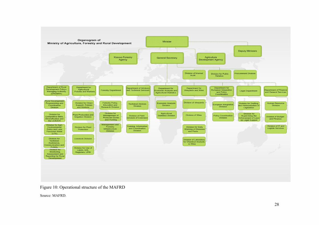
28

Figure 10: Operational structure of the MAFRD

Source: MAFRD.

29

Supported by the twinning project, the MAFRD prepared manuals on rules and procedures on

the functional structure of the MC, MA, manuals on programing, monitoring and evaluation, and

an organization chart and strategy for the further development of the PU. The MC, MA and PU

were established in accordance with the Law on Agriculture and Rural Development No.03/L-

098. In 2012, the PU was upgraded into the Paying Department (PD) which is now transformed

into the Paying Agency which is in full compliance with the Instrument for Pre-Accession

Assistance for Rural Development (IPARD) rules and procedures. The main duty of the PD is an

execution of the supported schemes drafted by the MA and funded by Kosovo’s Government,

bilateral and multilateral funds by the EU and other donor organizations. The Annual National

Program for Agriculture and Rural Development was the key implementation document of the

stated measures in ARDP 2007-2013. An implementation of the identified measures was also

supported with an extensive information campaign, aiming at the increase of farmers’ awareness

and promoting measures under the implementation.

An annual report of the Farm Accounting Data Network (FADN), annual monitoring and

implementation reports prepared by the MAFRD, respectively by the Division for Monitoring

and Evaluation and Paying Agency, are the key implementation and monitoring documents of

the ARDP. In September 2012, the MAFRD in cooperation with the Kastner International and

the Austrian Federal Institute of Agricultural Economics on behalf of the EU Twinning Project,

elaborated a Mid-Term-Evaluation (MTE) in implementing the ARDP. The MTE assesses all

implemented measures of the ARDP during the period of time 2007-2011. Based on the results

and recommendations drawn by the MTE as well as through an intensive discourse with socio-

economic partners, local action groups, agricultural producers and other organizations, the

MAFRD supported by the EU Twinning Project prepared the first draft strategy for the ARDP

2014-2020. On May 23rd, 2013 the draft strategy was firstly presented to the Steering Committee

and later on (3rd June, 2013) in conferences to all partners at interest. The conferences offered

valuable opportunities to engage the vast array of stakeholders and interest groups in discussions

and contributions to the agricultural policy debate and planning of the strategy for ARDP 2014-

2020. The Rural Development Policy of Kosovo 2014-2020 will be oriented according to the

new strategic directions of the EU Rural Development policy, by taking into consideration the

earned experiences during the ARDP 2007-2013 implementation as well as the Country Strategic

30

Paper Kosovo (09.2013). The stated objectives of the ARDP 2014-2020 are closely based on the

Instrument for Pre-accession Assistance II (IPA II) strategic policy objectives but also focus and

reflect country strategic objectives for development and specific needs of the Kosovo’s agri-food

sector, forestry and rural areas.

“Kosovo’s Rural Development Program 2014-2020 takes into account EU’s strategic objectives

for rural development and focuses on the following six priorities:

1) Fostering knowledge transfer for innovation in agriculture, forestry and rural areas;

2) Enhancing competitiveness in all types of agriculture and enhancing farm viability;

3) Promoting food chain organization and risk management in agriculture;

4) Restoring, preserving and enhancing ecosystems dependant on agriculture and

forestry;

5) Promoting resource efficiency and supporting the shift towards a low carbon and

climate resilient economy in the agriculture, food and forestry sectors;

6) Promoting social inclusion, poverty reduction and economic development in rural

areas”. (MAFRD, 2013).

The overall objectives of the ARDP 2014-2020 were defined as follows: “(i) to develop

competitive and innovation-based agrifood sector with an increased production and productivity

capable of producing high quality products and meeting the EU market standards, contributing to

the security and safety of the food supply, pursuing economic, social and environmental goals by

fostering employment and developing human and physical capital; (ii) to protect natural

resources and environment in rural areas, addressing the challenges of climate changes by

achieving sustainable and efficient land use and forestry management and by introducing

agricultural production methods which preserve the environment; (iii) to improve the quality of

life and diversify job opportunities in rural areas by fostering employment, social inclusion and

balanced territorial development of those areas”. (MAFRD, 2013).

The strategic objectives of the ARDP 2014-2020 will be achieved through an implementation of

the rural development priorities and measures under the EU IPA II and the National support

measures addressing income, land use and irrigation infrastructure financed by national budget

31

and donors initiatives. Table 12 presents the selected measures which will be implemented in

Kosovo, categorized under the four priorities of the EU IPA II for rural development.

Table 12: Selected measures to be implemented in Kosovo for the period of time 2014-2020

Priorities Measures

Enhancing farm viability and competitiveness Investments in the physical assets of

agricultural holdings;

Investments in the physical assets of the

processing and marketing of agricultural and

fishery products.

Restoring, preserving, enhancing ecosystems Agri-environmental measures and organic

farming;

Establishment and protection of forests.

Promoting social and economic inclusion Farm diversification and business

development;

Preparation and implementation of local

development strategies (LEADER).

Transfer of knowledge and innovation Improvement in training;

Advisory services;

Technical assistance.

Source: ARDP 2014-2020.

In out of nine selected measures, more than 60% of the ARDP resources will be allocated to the

measures under the priority one (enhancing farm viability and competitiveness). Budget

concentration into the priority one was based on strengths, weaknesses, opportunities, and threats

(SWOT) analysis of the Kosovo’s agriculture and food processing sector.

32

2.8 Agricultural policy measures main characteristics and changes 2007-2012 The allocation of the annual budget for agriculture and rural development is granted by the total

annual Kosovo consolidated budget. For the period of time 2008-2012, the average budget share

for agriculture and rural development out of the total public expenditures was 1.15%.

Table 13: Kosovo's MAFRD budget in million EUR, 2008-2012

Year 2008 2009 2010 2011 2012 Budget in € 8.6 13.9 14.2 15.0 25.0

Source: Ministry of Economy and Finance, 2008-2012.

Figure 11: Budgetary expenditure for agri-food sector in rural areas (million EUR)

Source: FAO/SWG. The aim of the direct support measures within ARDP was to increase agricultural production,

farmers’ income and to improve competitiveness of the agriculture sector relative to other sectors

and to import. Direct payments firstly started in 2008 with the support of fuel for harvesting as

input subsidy. In 2012, the allocated fund for the fuel support was 5.6% of the total expenses for

direct payments (MAFRD, 2014). No other input subsidies such as for fertilizer and pesticides or

0

2

4

6

8

10

12

14

16

18

2007 2008 2009 2010 2011

MISCELLANEOUS (not allocated)

GENERAL SERVICE SUPPORT

RDP MEASURES

MPS MEASURES

33

for seed and seedling were implemented for the period 2008-2012. Within direct producer

support measures the only supported measure was direct payment based on current cultivated

area with wheat seed, maize, oil plants, wine grape, payment per head of dairy cow, sheep, goats,

and beehives (MAFRD, 2014) .

Figure 12: Structure of the direct payments based on area/animal 2008-2012, Kosovo

Source: MAFRD, 2008-2012.

Of the total budget spent on rural development measures, more than 95% of the budget spent was

given for competitiveness and 1-2% on rural economy and population (Figure 13) (MAFRD,

2014). No founds were allocated for environment and countryside during the implementation of

ARDP 2007-2013.

0%

20%

40%

60%

80%

100%

2008 2009 2010 2011 2012

Payments for dairy cows Payments for ovine (sheep and goats)

Area payments for wheat Area payments for maize

Area payments for wheat seed Area payments for oil plants

34

Figure 13: Budgetary expenditure for rural development measures (million EUR)

Source: FAO/SWG.

Out of the total budget spent on competitiveness, more than 80% constituted farm restructuring

support (restructuring of the physical potential in the agri-rural sector, land consolidation,

managing water resources for agriculture and other on farm support) and 10-20% forestry

support (improving natural resource management) (Figure 13) (MAFRD, 2014). The structure of

the budgetary expenditure on competitiveness changed significantly in 2011 and 2012, where

more than 50% of the funds were spent on agri-food restructuring support (improving the

processing and marketing of agricultural products and establishment of collecting centers)

(MAFRD, 2014) .

0

1

2

3

4

5

6

7

8

9

10

2007 2008 2009 2010 2011

RDP- miscellaneous

Rural economy and population

Environment & countryside

Competitiveness

35

Figure 14: Budgetary expenditure for competitiveness (million EUR)

Source: FAO/SWG.

The initial implementation of the measure II on restructuring of the physical potential of the agri-

rural sector started in 2007 with the sub-measure II on milk. In 2012, out of the total budget

spent on measure II, 26.5% were allocated for sub-measure II (MAFRD, 2013). In 2008, the

MAFRD started with the implementation of sub-measures II on eggs, vegetables and vineyards.

The sub-measure II on vegetables covered the construction of new greenhouses, the expansion of

existing greenhouses and modernization of equipment/machinery and other infrastructure aiming

the improvement of quality and quantity of vegetable production. In 2012, this sub-measure had

the highest percentage share (29.4%) of the total budget spent on measure II (MAFRD, 2013).

Sub-measure II on vineyards aimed the improvement of quality and quantity of the table grape

production as well as the expansion of the cultivated areas with the table grape production. In

2012, the investment granted on the sub-measure vineyards was 2.5% of the total budget

expended on measure II (MAFRD, 2013). In 2009, out of the total sub-measures presented

within the measure II, the only supported measures were sub-measures on vegetables and

vineyards. In 2010, the MAFRD firstly started with the implementation of the sub-measure II on

fruits. The aim of this sub-measure was to increase the domestic production and quality of apple

and soft fruits. In 2012, the share of funds for this sub-measure was 20.9% of the total allocated

found for measure II (MAFRD, 2013).

0

1

2

3

4

5

6

7

8

9

2007 2008 2009 2010 2011

Miscellaneous

Forestry

Agri-food restructuring support

On farm restructuring

36

In 2008 and 2010, the measure on agricultural land consolidation was implemented through

capital investment projects. The aim of this measure was to improve the agricultural structure, to

build agricultural roads/paths and to protect land with a high level of biodiversity (MAFRD,

2013) .

The implementation of measure III on managing water resources for agriculture (axis 1 on

competitiveness) started in 2007 and was under implementation during the whole period of time

2007-2012. The aim of this measure was to increase the productivity and the quality of

agricultural products through the rehabilitation of the existing irrigation system as well as by

constructing new capacities. In 2012, the amount of the budget spent on this measure was 62.5%

lower compared to the previous year (MAFRD, 2013).

Measure IV on improving the processing and marketing of the agricultural products was under

implementation in the period of time 2010-2012. This measure supported construction of centers

for collecting, packaging and storing agricultural products. The measure covered dairy, meat,

grains, the fruits and vegetables subsector, bottled water, wine and beer. Support is meant to

improve the use of agricultural products through an enhancement of production of higher value

added, the establishment of collection centers, and the introduction of systematic preventive

approach to food safety Hazard Analysis and Critical Control Points (HACCP) in respect to food

safety, and of the production line and related facilities to meet EU requirements.

Since 2007, regular founds were allocated for improving natural resource management (measure

V). This measure was mainly focused on the reforestation of bare forest lands, and on monitoring

and maintaining afforested areas. In 2012, the amount of budget spent on this measure was twice

higher than the amount of budget expended in the previous year (MAFRD, 2013). According to

the Mid-Term Evaluation (MTE) report, problems related to the property rights and taking care

of saplings after planting need to be addressed rigorously to ensure that public money spent on

this measure is yielding results.

From 2009, the MAFRD started with the support of public and private projects which had an

impact on the improvement of living conditions of the rural population. Beneficiaries were Local

Action Groups (LAG) registered in Kosovo according to the LEADER principles. LAG

37

managers were responsible for the application and implementation of the projects that involve

rural community. Due to the budgetary constraints, farm diversification and alternative activities

in rural areas (measure VI) and improvement of rural infrastructure and maintenance of rural

heritage (measure VI) were not implemented at all in ARDP 2007-2013 (MAFRD, 2014).

From 2008 to 2012 more than 95% of the budget spent on general services comprised expenses

on food safety, particularly veterinary and phito-services, and a small percentage of the founds

was spent on research and development, advisory and expert services (MAFRD, 2013). The

measure on the development of vocational training to meet rural needs has been implemented

since 2008. The aim of this measure was to introduce new agricultural production technology,

environmental friendly production, and setting up networks and cooperation between farmers.

Training courses were delivered by contracted private companies in close cooperation with the

Municipal Agricultural Office (MAO). In 2012, the expended budget for vocational training was

by 65% higher than in 2011, while compared with the year 2008 it is about five times higher

(MAFRD, 2013). According to the MTE report vocational training measure contributed to an

increased agricultural production, more efficient use of farm inputs, and more specialized farm

activities (MAFRD, 2012).

38

3. LITERATURE REVIEW ON EFFICIENY

3.1 The efficiency concept and its interpretation The efficiency concept is considered to be a core of economics (Leibenstein, 1966). As a

criterion, it serves as bedrock for policy and planning approaches towards sustainable

development. The etymological origin of the English word ‘efficiency’ is derived from Latin

word ‘efficientia’ the present participle of the word ‘efficere’ meaning to accomplish, execute or

produce (Skeat, 1961).

The concept of efficiency has a wide range of interpretations and represents a multiplicity of

meanings derived from several disciplines such as thermodynamics, economics and lately

ecological theory, providing a rich mix of the efficiency concepts. An interpretation of the

efficiency term as “fitness or power to accomplish the purpose intended” (Simpson & Weiner,

1989) was taken from theological themes and in the context of the commercial activity of 18th

century Europe applied it more widely to the transient world (Jollands, 2003). As a result, the

key meaning of efficiency shifted from a theological basis to a logical positivist perspective

(Jollands N., 2006).

The importance of the efficiency criterion was raised and acknowledged with the substantial

increase of resource depletion and concerns for the efficiency of resource use. The term of

efficiency is omnipresent, and it has never been as prominent in our language as it is today

(Stein, 2001). In thermodynamic disciplines, energy efficiency is most commonly defined as the

ratio of the useable energy output to energy input (Patterson, 1996). The interpretation of the

economic efficiency measure is mostly related to the work of Vilfredo Pareto, to what is referred

now as allocative efficiency. Even within economic context, the term ‘efficiency’ does not

represent a single notion, rather it describes multidimensional interrelated concepts (Helm,

1988), which can be found in two main bodies of theory, namely production theory (technical

efficiency, production efficiency) and welfare economics (allocative efficiency, intertemporal

efficiency) (Jollands N., 2006).

39

“The world is complicated and no simple identity can capture everything” recognizing several

dimensions of the efficiency concept and integrating them into broader considerations is crucial

when analysing different aspects of the efficiency concept. In the principles of standard

economics, economy is seen as an “isolated system", which is useless for studying relationships

between economy and the environment (Daly, 1992).

Despite the multiplicity of meaning and the richness of the efficiency concept, for the purpose of

this study, its interpretation will be narrowed down within disciplinary boundaries. “In the

resource use context” potential interpretations of the efficiency term could be “from the ratio of

work output/energy inputs to Pareto efficiency” (Jollands N., 2006).

The theoretical foundations that do exist were developed and encouraged by the idea that

variation in efficiency might exist in some systematic fashion and be a phenomenon of

consequences (Grosskopf, 1985). In general, efficiency means obtaining the maximum amount

of output from a given set of resources, or production of a given output with minimum resources.

3.2 Economic Efficiency

Efficiency measurement and the interpretation of its behavior are of at most interest for business

firms and policy makers. Such measurements take the variety of forms in customary analysis

(e.g. cost per unit, profit per unit, etc.), and state them in the form of a OUTPUT/INPUT ratio

(Cooper W., 2002). Single factor indicator measurement (also called partial measurement) shows

the level of output produced by a asingle factor of production. It is estimated as the ratio of

output to the value of a single input (factor) considered. Commonly a single factor indicator is

calculated for labour and capital, as two types of output measures are used: gross output and

value added (Cooper W., 2002).

The main advantages of this indicators are: data is generally available (at firm, sector and

national levels), they are computed easily and can be used to determine the factor leading to the

efficiency improvement. But if not analysed in combination with the other indicators they can

40

produce misleading conclusions (Cooper W., 2002). Single input to single output measure can

mistakenly impute gain to one factor that is attributable to some other inputs (e.g. rising output

per worker may follow from additions to the capital stock) (Cooper W., 2002). Therefore,

moving from “partial efficiency measure” to “total factor measures” by taking into account all

outputs and all inputs, helps to avoid such problems and produces better indicator of the sector’s

efficiency. However, obtaining single input to single output ratios from all outputs and all inputs

poses some difficulties, such as the selection of inputs and outputs to be considered and the

weights to be used (Cooper W., 2002) .

The efficiency level varies depending on the production technology, production process and the

environment where the production is realized (Porcelli F., 2009). The producers are considered

to be efficient if they are able to produce as much output as possible with the inputs used and if

the output produced is at minimum cost (Greene, 1997). The efficiency measure is only one of

the components of performance measurement; the effectiveness is the other one that makes

overall performance measure complete (Figure15).

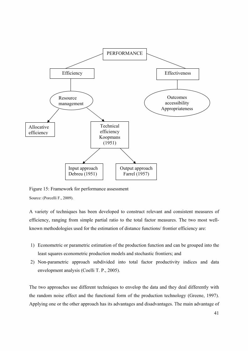
41

Figure 15: Framework for performance assessment

Source: (Porcelli F., 2009).

A variety of techniques has been developed to construct relevant and consistent measures of

efficiency, ranging from simple partial ratio to the total factor measures. The two most well-

known methodologies used for the estimation of distance functions/ frontier efficiency are:

1) Econometric or parametric estimation of the production function and can be grouped into the

least squares econometric production models and stochastic frontiers; and

2) Non-parametric approach subdivided into total factor productivity indices and data

envelopment analysis (Coelli T. P., 2005).

The two approaches use different techniques to envelop the data and they deal differently with

the random noise effect and the functional form of the production technology (Greene, 1997).

Applying one or the other approach has its advantages and disadvantages. The main advantage of

PERFORMANCE

Efficiency Effectiveness

Resource management

Outcomes accessibility

Appropriateness

Allocative efficiency

Technical efficiency Koopmans

(1951)

Input approach Debreu (1951)

Output approach Farrel (1957)

42

the econometric approach is that the method seeks the distinction between the effect of noise and

the effect of inefficiency. But as disadvantage is that it is a parametric method, meaning that it

requires specification of the functional form of production (Greene, 1997). A misspecification of

the functional form may lead to biased results of the efficiency scores (Barnes A.P., 2006). The

main advantage of the non-parametric approach is that it does not require this specification and

therefore is immune to misspecification of the functional form (Kelly E., 2012). The new

approach embodied in Data Envelopment Analysis (DEA) is that there is no need to prescribe

wights to be attached to each input or output, the variable weights are directly derived from the

data (Cooper W., 2002). On the other side, the non-parametric approach does not include error

term and it mixes the noise effect and the inefficiency effect under the voice of inefficiency

(Coelli T. P., 2005) but this problem can be exceeded using a bootstrapping method by (Simar

L., and Wilson W. P., 2007).

The method chosen for efficiency estimation also depends on the data availability. We used the

DEA approach and its models to measure the distance functions/efficiency scores. The

preference of DEA over the parametric approaches is that minimal assumptions are needed for

the frontier estimates. In addition, the DEA is a flexible technique that can easily fit the specific

purposes and needs of application as it approaches the valuation from a multidimensional

perspective.

3.3 Application of DEA in efficiency measure In recent years the DEA method has found a wide variety of applications from different entities

involved in many different kind of activities (Cooper W., 2002). It is considered to be one of the

most popular methods in operations research (Thanassoulis, 2001). It has offered a possibility for

identifying better benchmarks in many applied studies (Cooper W. W., 2011). In DEA, the

organization under study is called Decision Making Units (DMU) (Cooper W., 2002). In our

efficiency measurement, the DMU is considered a farm as an entity that converts inputs into

outputs. It is a linear programming optimization technique which measures the relative efficiency

of a set of comparable units. Another advantage of the method is that it can handle many outputs

43

and many inputs, relations (constraints) and loosens other requirements that come up when other

techniques are used (Cooper W., 2002).

According to (Koopmans T. C., 1951) definition of what is now called technical efficiency, a

feasible input-output vector is only technically efficient if it is technologically impossible to

increase any output and or reduce any input, without simultaneously reducing at least one other

output and or increasing at least one other input. Debreu (1951) was the first one providing an

index of the technical efficiency with his coefficient of resource utilization (Debreu G., 1951). It

is a radial measure of technical efficiency defined as one minus the maximum equiproportionate

reduction in all inputs consistent with continued production of given outputs (Debreu, 1951).

Farrell (1957) is considered to be the most influential by extending Koopmans and Debreu’s

work and was the first one to decompose overall efficiency into technical and allocative

efficiency. Farrell’s technical efficiency refers to the estimated efficiency measure based on the

physical relation of inputs and outputs used in the production function. For a ‘perfectly efficient

firm the efficiency takes the value of unity or 100 per cent and it might become indefinitely small

if the quantity of input per unit output become indefinitely large (Farrell, 1957).’ Initiated by the

Farrell’s work, the DEA became a new tool for measuring technical efficiency when Charnes,

Cooper and Rhodes (1978) proposed the initial DEA model known as CCR model (Cooper W.,

2002). The efficiency measure under the CCR model is obtained ‘as the maximum ratio of

weighted outputs to weighted inputs subject to the condition that similar ratios for every DMU

will be less than or equal to unity’ (Charnes A. C., 1978), which takes the form as presented in

the equations below:

(1)

∑

∑

subject to:

∑

∑ 1;

44

1,… . , ; , 0; 1, … . , ; 1, … . , . Where, , are known outputs and inputs of the j DMU; , 0 are wights to be assigned

by the problem solution (Charnes A. C., 1978). The fractional linear program can be converted

into linear form and the methods of linear programming can be applied (Boussofiane A., 1991).

Therefore, the fractional program of CCR is equivalent of a linear program (Cooper W., 2002)

which can be solved in n linear programs, one for each DMU (Charnes A. C., 1978).

(2)

subject to:

0, 1, 2, … . ,

1,

0 1, … , ,

0 1, … , .

The objective function of input-oriented approach of the CCR model is to minimize inputs while

keeping the outputs levels constant, whereas the output-oriented approach seeks maximizations

of the outputs with no additional inputs used (Cooper W., 2002). The two versions of the CCR

model were developed under the assumption of Constant Returns to Scale (CRS). Under such

45

assumption the activity (x, y) is feasible when, for every positive scalar t, the activity (tx, ty) is

also feasible (Cooper W., 2002). It means that a proportional increase in the input level will

proportionally increase the output level (Toloo M, and Nalchigar S., 2009).

Later the CCR model was extended by Banker, Charnes, and Cooper (1984) to a new model

known as BCC model, which estimates pure technical efficiency of the DMU-s (Toloo M.,

2009). The frontiers in the BCC model have piecewise linear and concave characteristics which

leads to Variable Returns to Scale (VRS) allowing identification of a DMU that it is performing

in increasing, decreasing, or constant returns to scale (Cooper W., 2002). ‘Increasing Return to

Scale (IRS) prevail if β > α, and Decreasing Returns to Scale (DRS) prevail if β < α (Cooper W.

W., 2011).’ Banker et al. (1984) and Banker and Thrall (1992) extended the concept of returns to

scale from single output case to multiple-output using DEA (Cooper W. W., 2011).

The BCC model (Banker RD., 1984) assumes n DMU-s, (DMUj: j = 1, 2,…, n) use m inputs (xi: i

= 1, 2,…, m) to produce s outputs (yr: r = 1, 2, …., s). The BCC input and output-oriented

approaches take forms as presented in the equation 3 and 4:

(3)

subject to

0, 1, 2, … . ,

1, ,

46

(4)

0, 1, 2, … . ,

1, ,

Where xij and yrj (all non-negative) are the inputs and outputs of the DMUj, wi and ur are the

input and output weights, xio and yro are the inputs and outputs of DMUo.

CRS

VRS

D

A

C

x

B

y

Figure 16: Production frontier of the single input and single output under CRS and VRS

assumption for the DMUs A, B, C, and D

Source: (Ortner K., 2006).

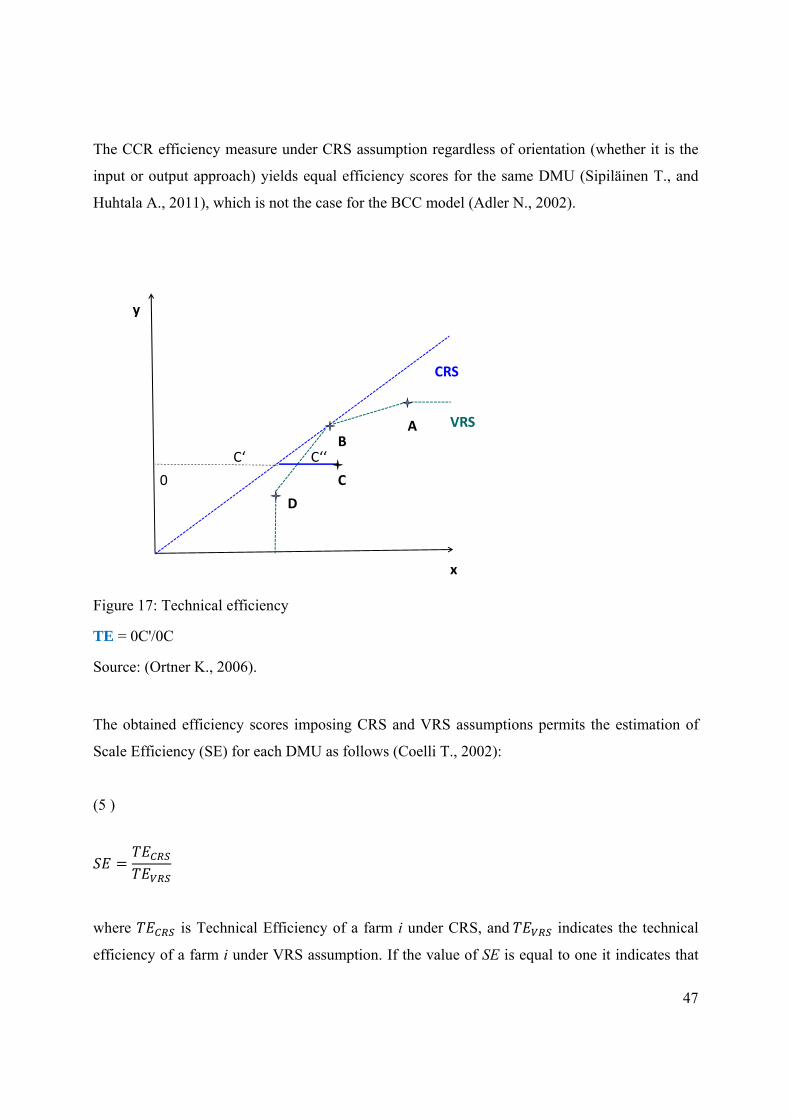
47

The CCR efficiency measure under CRS assumption regardless of orientation (whether it is the

input or output approach) yields equal efficiency scores for the same DMU (Sipiläinen T., and

Huhtala A., 2011), which is not the case for the BCC model (Adler N., 2002).

CRS

VRS

D

BA

C

x

0

C‘ C‘‘

y

Figure 17: Technical efficiency

TE = 0C'/0C


The obtained efficiency scores imposing CRS and VRS assumptions permits the estimation of

Scale Efficiency (SE) for each DMU as follows (Coelli T., 2002):

(5 )

where is Technical Efficiency of a farm i under CRS, and indicates the technical

efficiency of a farm i under VRS assumption. If the value of SE is equal to one it indicates that

48

the farm is operating at an optimal scale and at SE ˂ than one farm is scale inefficient and this

may come either due to the existence of IRS or DRS. The estimated technical efficiency scores

imposing Non Increasing Returns to Scale (NIRS) TENIRS provides an indication if the scale

inefficiency is due to the DRS which means that farm is larger than optimal scale (TENIRS =

, or as a result of the IRS, meaning that the farm is operating at smaller scale than optimal

(TENIRS ≠ ) (Coelli T., 2002).

CRS

VRS

D

BA

C

x

0 C‘‘

y

Figure 18: Pure technical and scale efficiency

Pure Technical Efficiency (PTE)= 0C‘‘ / 0C

Scale Efficiency (SE) = 0C‘ / 0C

TE = SE * PTE


Based on the basic models of CCR and BCC, other DEA models have been developed and

appeared in the literature (Cooper W W., 2000). The extended DEA models used different

assumptions related to the nature of returns to scale in the production frontiers. Shortly after the

BCC model's appearance, (Charnes A., 1985) introduced additive models to the DEA. The

49

additive models treat the slacks (the input excesses and output shortfalls) directly in the objective

function and combine input and output-oriented models into a single model (Cooper W., 2002).

According to the additive model definition the DMU is only fully efficient if there are zero

slacks in both inputs and outputs used in the production function (Cooper W., 2002). Thus, a

weakly efficient DMU (referring to Farrell’s efficiency) will be evaluated as an inefficient DMU

in the additive models, due to the presence of input or output-oriented slacks (Adler N., 2002).

Other features of the additive models are coordinate-free and are invariant in regard to the

translation of the coordinate system (Cooper W., 2002), but have no scalar measure (ratio

efficiency) (Tone K., 2001).

Another model for measuring the efficiency with a close connection to CCR and BCC models is

a Slacks Based Measure (SBM) of efficiency (Tone K., 2001). Earlier attempts were made by

Russell, 1988; Lovell and Pastor, 1995; Cooper and Pastor, 1997; Cooper and Tone, 1997 to

evaluate inefficiency based on slacks (Tone K., 2001). The SBM measure is interpreted as a

product of input and output inefficiencies; it also allows for adding in economic aspects

(information on costs and prices) since the model maximizes the virtual profit instead of virtual

ratio of the CCR model (Tone K., 2001).

The cross-evaluation matrix was firstly developed in 1986 by Sexton et al. (Adler N., 2002).

Later, Doyle J. and Green R. elaborated understanding of cross-efficiency in the concept of peer-

appraisal, differently from self-appraisal by simple efficiency (Doyle J., and Green R., 1994).

‘The cross-efficiency measure uses the set of weights chosen for a particular DMU to weight the

inputs and outputs for each of the other DMUs and calculates the cross efficiency of each of the

other DMUs based on the original DMU (Doyle J., and Green R., 1994).’ Doyle and Green

stressed out that the cross-efficiency method as a peer-appraisal has less of the arbitrariness of

additional constrains and is considered to be more connected to democratic process compared to

the simple efficiency (self-appraisal). Its main advantages are: (a) ability to order DMUs and (b)

the possibility to eliminate unrealistic weight schemes with no placement of weight restrictions

from application area experts (e.g. Anderson et al. 2002) (Cook D.W., and Zhu J., 2015). The

cross-efficiency measure is mainly used as a complementary method to the simple efficiency,

rather than in pure self-evaluation mode (Cook D.W., and Zhu J., 2015).

50

A new method for ranking the efficiency of DMUs called super-efficiency was developed by

Andersen and Petersen (1993). The super-efficiency model is similar to the BCC model, with the

difference that the DMU under evaluation is not included in the reference set (Anderesn P., and

Petersen N., 1993). This method allows distinction between efficient and inefficient units; the

unit under assessment is compared to a point in the efficient subset created from all other

observations in the sample (Anderesn P., and Petersen N., 1993). The index obtained through

this method can be interpreted as ‘the maximum possible proportional decrease in the input

vector nedeed to make the observation efficient’ and it can takes the values equal to or larger

than one for the efficient observation (Anderesn P., and Petersen N., 1993). Some issues were

raised in regard to the methodology used in supper-efficiency estimation, e.g. giving

“specialized” DMUs an excessivelly high ranking or the problem of infeasibility, meaning that if

it takes place, the super-efficiency technique can not give a complete ranking of all DMUs

(Adler N., 2002). In regard to the first concern (high ranking), Sueyoshi (1999) set up specific

bounds on the weights in the super-efficiency ranking method, whereas, concerning the problem

of infeasibility, Sueyoshi (1999) limited the super-efficiency scores to a scale with a maximum

of 2 by introducing an Adjusted Index Number (Adler N., 2002).

In addition to the models presented so far, other DEA models were developed and introduced to

the subject of efficiency ranking units e.g. Torgersen et al. (1996) developed a method for the

complete ranking of efficient DMUs through measuring their importance as a benchmark for

inefficient DMUs (Adler N., 2002). Others, like Zhu (2003a, 2009) provided DEA models which

are useful in performance evaluation and benchmarking (Cooper W. W., 2011). The DEA

method was also extended to another new model called Imprecise DEA (IDEA) which allows

treating not only the exact data but also imprecise data which are known only ordinally or within

prescribed bounds (Cooper WW., 2001). Moreover, Cooper et al. (2001) demonstrated ‘how

conditions on the variables (Assurance Region (AR-IDEA) as in Thomson et al. 1990, 1995) as

well as the data, including variable-data transformations as applied by Charnes et al. (1990) in

the cone-ratio envelopment, could be treated in the same manner.’

51

An additional approach which deals with the imprecise inputs and outputs in DEA models is the

‘fuzzy DEA’ method (Lertworasirikul S., 2003). This method takes the form of fuzzy linear

programming which is assisted by other methods to rank fuzzy sets i.e. the possibility approach

which transforms fuzzy DEA models into possibility DEA models where constraints are treated

as fuzzy events (Lertworasirikul S., 2003). In an attempt to narrow the gap between DEA and the

classical statistical approaches, many other additional methods were introduced and used in

efficiency ranking of the units under the study e.g. ‘multivariate statistics in the DEA context,

canonical correlation, linear discriminant, discriminant analysis of ratios for ranking, DEA and

multi-criteria decision making units (Adler N., 2002).’

3.4 Environmental Efficiency

3.4.1 Definition and concept of externalities

Economic value of a good is revealed and takes place in the market, but in many cases

contribution of the environmental goods and services are not channeled via functioning markets

and are missing markets (Pearce D. & Barbier E., 2000). Market competition leads to some

extent of social optimality. However, perfect market competition fails to fulfill some of the

imposed specific assumptions associated with rivalry, excludability, appropriability and

externalities (Just R., 2004). Therefore, public policy intervention can potentially improve the

market's allocation and reach Pareto optimality.

‘The economic assumptions to which the proofs of efficiency called attention concerned the

absence of externalities and public goods (Szenberg M. & Ramrattan L., 2004).’ A pure public

good is a good that is both non-excludable (once a good is available for consumption by one

individual, then others cannot be excluded from consuming it) and non-rival (the consumption of

the good by one individual does not prevent other individual’s enjoyment of consuming that

good) (Just R., 2004).

A pure private good is considered to be a good the production or consumption of which does not

destruct or help individuals that are not directly involved in its production or consumption

(Mankiw G., 2000). However, some private goods cannot be considered as pure private goods as

52

they do comprise externalities (Mankiw G., 2000). In the presence of externalities, society’s

interest in a market outcome includes the well-being of bystanders affected from buyers and

sellers in the market (Mankiw, N. G., 2007). An externality occurs when a person or economic

agent engages in an activity that influences the well-being of another and yet does not pay or

receive any compensation for that effect (Mankiw, N. G., 2007).

Figure 19: Classification of external effects

Source: (Bator, 1958).

The figure 19 shows the classification and the direction that the externalities can be imposed

from producers to consumers, consumers to consumers, consumers to producers and producers to

producers (Just R., 2004). It also indicates that externalities in one way can be associated with

the production of goods but also with the consumption of goods and services. The most well-

known external effects that received a lot of attention are those on consumers caused by

producers (Just R., 2004). Whereas, in terms of the variety, externality may be adverse, in which

case it is called a negative externality or beneficial, known as positive externality (Just R., 2004).

53

Figure 20: Negative externality in a single commodity market

Figure 21: Positive externality in a single commodity market

Source: (Mankiw, N. G., 2007). Source: (Mankiw, N. G., 2007).

In the case of negative externality (Figure 20) the market equilibrium quantity (Q Market) is

larger than the socially optimal quantity (Q Optimum), and this inefficiency takes place as the

market equilibrium considers only the private costs of production (Mankiw, N. G., 2007).

Therefore, the overproduction of goods that generate negative externalities happens as the

marginal private costs of production are lower than the marginal social costs of production

(Mankiw G., 2000). Some of the negative externalities are often due to the presence of ‘common

pool resources’ which leads to the situation of over used resources (e.g. community owned

pastures) (Mankiw G., 2000). Comparable to the previous figure, in the case of positive

externality (Figure 21), the social cost of production reflected in the supply curve is lower than

the private (Mankiw, N. G., 2007). As the marginal private benefit is lower than the marginal

social benefit, there is less incentive to generate positive externalities, which therefore are

generally under supplied by the market (Mankiw G., 2000).

There are various actions taken by private actors and public policymakers in response to the

externalities. In some situations, the problem of externalities is solved with moral codes and

social sanctions (private solution) (Mankiw, N. G., 2007). But private negotiation does not

adequately internalize all types of externalities without government intervention (Stavins R.,

54

2004). The Coase theorem (private solution) approach assumes that there are zero transaction

costs, no income effects, private goods (not public goods) and no third party impacts (Revesz R.

& Stavins R., 2004). Such assumptions are questioned, particularly from environmental scientists

and are often considered as virtually impossible (Rutherford D., 2007). In public policy, there are

mainly two types of policy approaches to the problem of externalities; the first one is the market

failures approach that follows the work of neoclassical economist Arthur Pigou (1932), which

aims to identify such externalities and internalize them through regulatory measures e.g.

command control, tradable emission permits, taxes for negative externalities and subsidies for

positive externalities (Oates W. & Portney P., 2003); and the second one is associated with the

‘Chicago School’ of economists and focuses on the creation and distribution of clearly defined

‘property rights’ (Hodgson G., 1999). Each of these two approaches face inherent difficulties in

addressing the problem of externalities; Pigovian's approach needs detailed expert information

on externalities that often is difficult to obtain, while the property rights approach often has a

deficiency of clearly defined property rights (Hodgson G., 1999). In addition to the economic

instruments, non-economic instruments, communicative policies and a combination of all (e.g.

agri-environmental schemes), there are other sets of instruments which are used to compensate

for market failures (Schader Ch., 2009).

Agriculture in addition to its multifunctional role associated to economic, food security, social

and cultural role (FAO, 1999), also affects other multiple ecosystem functions e.g. biodiversity,

water and soil quality (Waldhardt R. et al., 2010). Such functions are considered to be

unintended by-products, or externalities generated by agriculture, the economic values of which

markets do not take into account (FAO, 2001). Unlike other sectors, agriculture can produce both

positive and negative environmental externalities, and this depends on the demand for its

products. e.g. to a large extent on farmer production practices (Hayo M.G. van der Werf and

Petit J., 2002). Agriculture intensification contributes to the loss of biodiversity or increases

water pollution through the emission of agro-chemicals and animal waste (Blandford D., 2011).

For most of these externalities farmers do not directly bear any costs for generated negative

externalities or directly benefit from positive externalities (Cooper J. C., 2001). The unintended

agriculture externalities have an impact on people other than the producer of that externality

(Cooper J. C., 2001). Therefore, agriculture policy makers should find out if agriculture gives

55

more or less of the positive or negative externalities than the land use pattern that would exist

without policy intervention (Cooper J. C., 2001).

Table 14: List of frequently cited positive and negative externalities provided by agriculture

Environmental amenities

(positive externalities)

Environmental disamenities

(negative externalities)

Open space, scenic vistas, isolation from

congestion, watershed protection, flood

control, ground water recharge, soil

conservation, biodiversity, wildlife habitat.

Odour, nutrient/pesticide runoff, reduced

watershed protection, reduced flood control,

soil erosion, biodiversity loss, wildlife

habitat loss.

Source: (Cooper J. C., 2001).

Many studies have been focused on negative externalities generated from agriculture (e.g.

Weaver R.D., 1997; Weaver R.D. and Kim T., 1999; Reinhardt S. A. et al., 2000; Hayo M.G.

van der Werf and Petit J., 2002; Ball V.E et al., 2004; Garcia A.F and Shively G. E., 2010; Ullah

A. and Perret S.R., 2014). However, few studies considered positive externalities produced by

agriculture (e.g. Sipiläinen T. et al., 2008; Solovyeva I. and Nuppenau E.A., 2012), and they did

not appear until the 1980s, when the Japanese pioneered allocating monetary values to rice

paddies (Soda O., 2003).

The total economic value of a good or service consists of two main components: 1) its use value

(the value derived from its direct use); and 2) the non-use value which involves no actual

interaction between people and the environment and can be the value given for its existence,

inheritance value (the value given by current generation from knowing that the resource is

conserved for future) and option value (future use value) (Mendelsohn R. & Olmstead S., 2009).

56

Figure 22: Typology of the total economic value approach

Source: (Brander L., Gómez-Baggethun E., Martín-López B., Verma M., 2010).

3.4.2Methodsforassessingagricultureexternalities

Due to the socio-demographic and environmental differences, weights given to the positive or

negative externalities by society differ among the developed and developing countries (Cooper J.

C., 2001). In general, their economic value tends to be unknown as they do lack a developed

market and do not have prices in the market (FAO, 2001). This situation compelled

environmental economists to use non-market valuation techniques to estimate the economic

value of environmental costs and benefits (Feather P., 1999). The most common methods used in

the valuation of the environmental goods and services can be grouped in:

1. Direct market valuation methods;

2. Revealed preference methods; and

3. Stated preference methods;

57

The direct market valuation methods use different approaches such as (a) market price-based

approaches, (b) cost-based approaches, and (c) approaches based on production functions

(Brander L., Gómez-Baggethun E., Martín-López B., Verma M., 2010). The market price-based

approach is usually used to attain the value of provisioning services, as goods produced by

provisioning services are sold on the market (Brander L., Gómez-Baggethun E., Martín-López

B., Verma M., 2010). The cost-based approach estimates the raised costs if ecosystem service

benefits needed to be recreated from artificial means and it includes the avoided cost method,

replacement cost method and restoration cost method (Garrod, 1999). The approaches based on

the production function, estimates the contribution of ecosystem services to the improvement of

economic welfare or productivity (Pattanayak S. & Kramer R., 2001), or the contribution of a

given ecosystem service to the delivery of a commodity tradable in the market (Brander L.,

Gómez-Baggethun E., Martín-López B., Verma M., 2010). The main advantage of these methods

is that they are based on the market's data e.g. prices, quantities and costs, which are available

and rather easy to obtain (Brander L., Gómez-Baggethun E., Martín-López B., Verma M., 2010).

However, the use of such methods is limited, particularly in the evaluation of environmental

goods and services that do lack data in the market. Therefore, the policy decisions based on such

methods can lead to wrong decisions as they can provide biased and not reliable information

(Barbier E. B., 2007).

The revealed preference methods are based on the observation of individual choices in actual

markets associated to the ecosystem service in the focus of valuation (Brander L., Gómez-

Baggethun E., Martín-López B., Verma M., 2010). This group of methods consists of different

models such as (a) travel cost models, (b) hedonic property models, (c) hedonic wage models

and (d) averting behavior models (Mendelsohn R. & Olmstead S., 2009). The travel cost method

uses the travel costs people have to pay traveling to the sites and it is utilized as a proxy for the

unobservable price of natural resource (Kriström B., 1990). Travel cost models build the demand

function for any good or service based on the empirical relationships between travel cost and

visitation rates (Clawson M., 1959). Travel cost models are very popular and widely used in the

valuation of recreational demand which is an important part of the total economic value for many

natural goods and services (Mendelsohn R. & Olmstead S., 2009). It is considered to be a more

objective valuation method, but also has limitations as it is applicable only in cases where people

in one way or another already pay for the environmental goods and services (Brander L., Gómez-

58

Baggethun E., Martín-López B., Verma M., 2010). The main weak point of such models is that

many important factors are left out and therefore the generated results can be biased e.g.

opportunity cost of a travel time or multipurpose trips (Mendelsohn R. & Olmstead S., 2009).

The hedonic pricing approach uses the price of a good compounded from a sum of the implicit

prices for each characteristic of the marketed commodity e.g. the change in the value of a house

situated in a view on a nice landscape reflects the value of a change in biodiversity or ecosystem

services (Brander L., Gómez-Baggethun E., Martín-López B., Verma M., 2010). The Ricardian

model of agricultural land is one of the hedonic property approaches that evaluates the effect of

climate on the value of a farm land (Mendelsohn R. & Olmstead S., 2009). The averting behavior

models employ the avoidance costs of people to partially estimate the value of the damages from

pollution (Mendelsohn R. & Olmstead S., 2009). The hedonic property and wage models are

mainly suitable for work-related hazards and for assessing the impact of environment on

property values, whereas averting behavior models are mostly utilized in evaluating the effect of

pollution on peoples’ health (Barbier E. B., 2007). The revealed preference methods are

incapable of assessing non-use values, which is considered to be the main disadvantages of such

methods (Kontoleon A., 2007). In addition, the technical assumptions made about the

relationship between the environmental good and the surrogate market good, create a

dependency of the estimated values (Kontoleon A., 2007).

The stated preference methods create hypothetical markets in order to obtain the values through

the use of a designed surveys that asks directly individuals how much they are willing to pay for

the value of environmental goods and services (Mendelsohn R. & Olmstead S., 2009). The stated

preference methods include (a) contingent valuation methods, (b) conjoint analysis and (c)

choice experiments (Barbier E. B., 2007). The contingent valuation method starts with the clear

description of the amenity considered for evaluation and the policy change suggested; it proceeds

with a set of choice questions that ask an individual to set a value on the amenity, followed by

the assessment of a set of questions associated to the socioeconomic characteristics of the

individual that could potentially explain the variation of the stated value (Young RA., 2005). The

contingent valuation method relies on the subjective valuation of the environmental issues, as it

asks respondents directly about their willingness to pay for the environmental goods and services

(Kriström B., 1990). The advantages of the stated preference methods are their ability to value

environmental goods and services at levels of quality that are currently not existing and the

59

possibility to detain non-use values (Mendelsohn R. & Olmstead S., 2009). However, difficulties

are faced in the implementation phase of such methods, as giving the values on natural

ecosystem services requires information that allows a clear description of the changes of services

that people care about (Heal G.M., 2005). In addition, understandable explanations of the survey

instrument must be supplied, so people may become more familiar with valuation of changes in

natural ecosystem services and do not reject the valuation scenario (Heal G.M., 2005).

3.4.3 The DEA method for environmental performance valuation

The measurement of environmental performance at micro and macro level has recently received

great attention due to the increased concern associated with environmental issues and sustainable

development (Zhou P., 2016). A ‘non-parametric approach can easily take on the derivation of

environmental performance indicators into efficiency measures (Tyteca D., 2006).' Therefore, the

DEA is considered to be a useful alternative method for environmental performance valuation of

the units at different levels. In comparison to its use in other fields, such as applied economic

sciences, agricultural economics, development economics, financial and public economics, its

application in the field of environmental economics was less widely dispersed (Kuosmanen T. &

Kortelainen M., 2004). In traditional measure of the productivity and efficiency, the joint

production of good and bad outputs is usually ignored due to the absence of prices for such

outputs (Chung H. Y., Färe R. and Grosskopf S., 1997). In this regard, the advantage of the DEA

method is that it allows inclusion of variables of different nature (independent of units

measurement) (Lovell K., and Pastor J., 1995), and of the outputs without the presence of

market, hence without price, such as the generation of employment, quality indicators and

environmental measures (Antonio F. Amores F.A. and Contreras I., 2009). The unique valuation

feature of the DEA method is that it is independent of stated or revealed preferences, as it turns

the value problem the other way around and asks what kind of prices would favour that particular

good or service (Kuosmanen T., 2009). In the conventional DEA models, all outputs are assumed

to be desirable outputs (producing more outputs given the constraints of inputs) whereas, this

assumption does not hold in the case of undesirable outputs and it needs to be differently

incorporated into the DEA (Zhou P., 2016). Cropper and Oates used economic arguments to treat

60

detrimental variables as inputs, as both inputs and detrimental variables convey costs for a firm

and commonly the interest of firms is to decrease both types of variables (Kuosmanen T., 2005).

In the frame of the DEA method different approaches were developed and used in regard to the

inclusion of desirable and non-desirable outputs into the economic-environmental context

analysis. The approaches which treat undesirable outputs as inputs can be grouped in two

methods: (1) methods based on the translation invariance, where undesirable outputs are

multiplied by “-1” and after adding to the value obtained a number which is sufficient to make

all the undesirable outputs positive; (2) methods based on the concept of weak disposable

reference technology introduced by Färe et al. (1989) (Zhou P., 2016). In the Färe et al. (1989)

approach, the undesirable outputs were modelled either as weakly disposable outputs or as inputs

(Sipiläinen T., and Huhtala A., 2011). Weak disposability means that there are possibilities to

decrease emissions of undesirable outputs and other detrimental side-effects, through decreasing

production activities (Kuosmanen T., 2005). Whereas, on the technical side, emissions to the

environment usually are considered as outputs for a company (Kuosmanen T., 2005).

The extended Färe et al. (1989) hyperbolic efficiency measure allowed to obtain an

equiproportionate increase in desirable outputs while reducing the level of undesirable outputs

(Reinhard S., 1999). The approaches by Färe et al., (1993) and Hetemäki (1993) revealed

technical efficiency scores and shadow prices for undesirable outputs through a Trnaslog output

distance function estimation (Mulugeta E., 2013). Lovell et al. (1995) used the reciprocal of the

undesirable output as DEA output which means ‘the undesirable output is modeled as desirable

(f ( 1/ , where is one of the elements of the matrix U of the undesirable outputs i

of the DMU k (Gomes EG., and Lins MPE., 2007).’ Rheinhard et al. (1999) calculated a non-

radial environmental efficiency index estimated as the input oriented technical efficiency of a

single detrimental input (e.g. nitrogen surplus from a farm) (Reinhard S., 1999). For additive and

BCC models Ali and Seiford (1990) have demonstrated how ‘the translation of the data values

does not change the efficient frontier and therefore the ranking of DMUs is translation invariant

(Ali I. A., and Seiford M. L., 1990).’ Sheel (2001) incorporated undesirable output as a normal

output after the transformation of the data (Sipiläinen T., and Huhtala A., 2011). In DEA, there

are three cases of invariance in data transformation: (1) classification invariance, (2) ordering

61

invariance, (3) solution invariance (Seiford M. L., and Zhu J., 2002). Seiford and Zhu based on

the first case of invariance ‘classification invariance’ developed a model which incorporates

desirable and undesirable factors under the context of the BCC model.

The estimation of environmental DEA technology is more widely applied in modeling

environmental performance e.g. Zhou P., 2016; Solovyeva I., and Nuppenau A. E., (2013);

Sipiläinen T., et al. (2008); Kiatpathomchai S., (2008); De Koeijer et al. (2002) etc. In the

environmental DEA efficiency measures most of the studies assume technology that show

constant returns to scale (Zhou P, 2006). However, there are cases where production technology

exhibits variable returns to scale (Tyteca D., 2006). Tyteca (1996) adopted an aggregated

concept into the DMU environmental performance and emphasized that the developed models

would be inadequate at the process or product level such as those in the life cycle analysis or for

the companies that simply have to report their environmental impacts to the environmental audit.

Concerning the environmental DEA technology measures imposing variable returns to scale

assumption other authors (Scheel H., 2001) and (Färe R. and Grosskopf S., 2004) developed

models that allow joint environmental technology measures. Scheel (2001) concludes that in the

new “nonseperated” measures the DMUs will be less efficient as compared to the trigonal

measures which treats desirable and undesirable variables separately.

Mainly, most of the environmental DEA models incorporate undesirable outputs into the classic

Farrell's framework of the efficiency analysis, thus by adding the quantities of these detrimental

variables denoted by vector w, to the general production possibility set

, | , this production possibility set can be

redefined as , , | (Kuosmanen

T. & Kortelainen M., 2004). There are different orientations (environmental, input-

environmental, output-environmental, hyperbolic, and directional) used in the measurement of

environmental performance as distance to the environmental technology (Kuosmanen T. &

Kortelainen M., 2004). When it comes to the choice of orientation, Kuosmanen and Kortelainen

emphasize that it is advisable to consider constant factors that the firm cannot control and

decrease or increase factors which are under the firm’s control. Other measures or indicators in a

more aggregated method were suggested for measuring environmental or eco-efficiency e.g. Net

62

Value Added (NVA) which indicates the difference between annual Value Added (VA) and the

Value Lost (VL) which gives environmental performance indicator as ɛ=NVA/VA, pollution

performance index of a firm, pollutant risk, pollutant intensity index, overall pollution index etc.

(Tyteca D., 2006). Eco-efficiency can be attributed to commodities and also organizations and it

means ‘producing outputs with less natural resources and environmental degradation’

(Kuosmanen T., 2005). Another approach which is different from the environmental

performance measures of production economic approaches was developed by Kortelainen M.

and Kuosmanen T. (2004). This approach is more ecologically oriented as it focuses on

environmental pressures rather than specific undesirable outputs and it is defined as ‘production

activity is eco-efficient if and only if it is not possible to decrease any environmental pressure

without simultaneously increasing another pressure or decreasing the economic value added’

(Kortelainen M., and Kuosmanen T., 2004). Following this definition, Kortelainen and

Kousmanen's eco-efficiency measure was presented as the ratio of economic value added to the

index of environmental pressure denoted as D (Zn). The D (Zn) index was constructed by using

benefit of the doubt weighting scheme which gives weights that maximize the relative eco-

efficiency of the evaluated activity compared to the maximum potential eco-efficiency

(Kortelainen M., and Kuosmanen T., 2004).

63

4. DATACOLLECTIONANDDESCRIPTIVESTATISTICS

4.1Thestudyarea Kosovo is a small country with a total area of 10,908 km2, situated in the center of the Balkan,

between the Mediterranean Sea and the mountainous regions of Southeast Europe. According to

the latest census conducted in 2012, the country’s total population, which is the youngest in

Europe (with an average age of 30.2), was counted at 1,815,606 inhabitants. Compared to other

Western Balkan countries Kosovo has the highest population density (177.4 inhabitants/km2).

The majority of the population (61%) is living in rural areas and the average household size in

2012 was estimated to be 5.85 members.

Kosovo lies between N43°16´; S41°53´; E21°16´; W19°59´ and is divided in two main plains,

the Dukagjini plain in the west and the Kosovo plain in the east. The lowest point of altitude is

265 m above the sea level located at "Drini i Bardhë" at the border to Albania and raises up to

2,656 above the sea level which is located in the southern part of Kosovo called Gjeravica. In

total, approximately 80% of the entire area lies below 1,000 m. On June 2008, the Assembly of

Kosovo adopted the Law No.03/L-041 on Administrative Municipal Boundaries and on the basis

of this law the country composes of 5 regions, 38 municipalities and 1,469 settlements (KAS,

Statistical Yearbook of the Republic of Kosovo, 2014).

The Kosovo plain embraces the Ibar Valley which is influenced by continental air masses.

Therefore, winters in the Kosovo plain are much colder when compared to the Dukagjini plain,

which is influenced by air masses which cross the Adriatic Sea, and the temperatures during the

winter seasons vary between –10 °C down to –26 °C. The summers are usually very hot and the

temperatures vary in from 20 °C up to 37 °C. The climate in the Kosovo plain is moderately dry

with an average annual precipitation of 600 mm per year. In the Dukagjini plain, winters are

milder and the monthly mean temperatures vary in the range of 0.5 °C up to 22.8 °C. The

average annual precipitation of the Dukagjini plain is about 700 mm per year.

According to a digital map on soil types (scale 1:50000) produced by the Chair of Soil Science

of the University of Prishtina “Hasan Prishtina” and referring to the WRB-soil classification

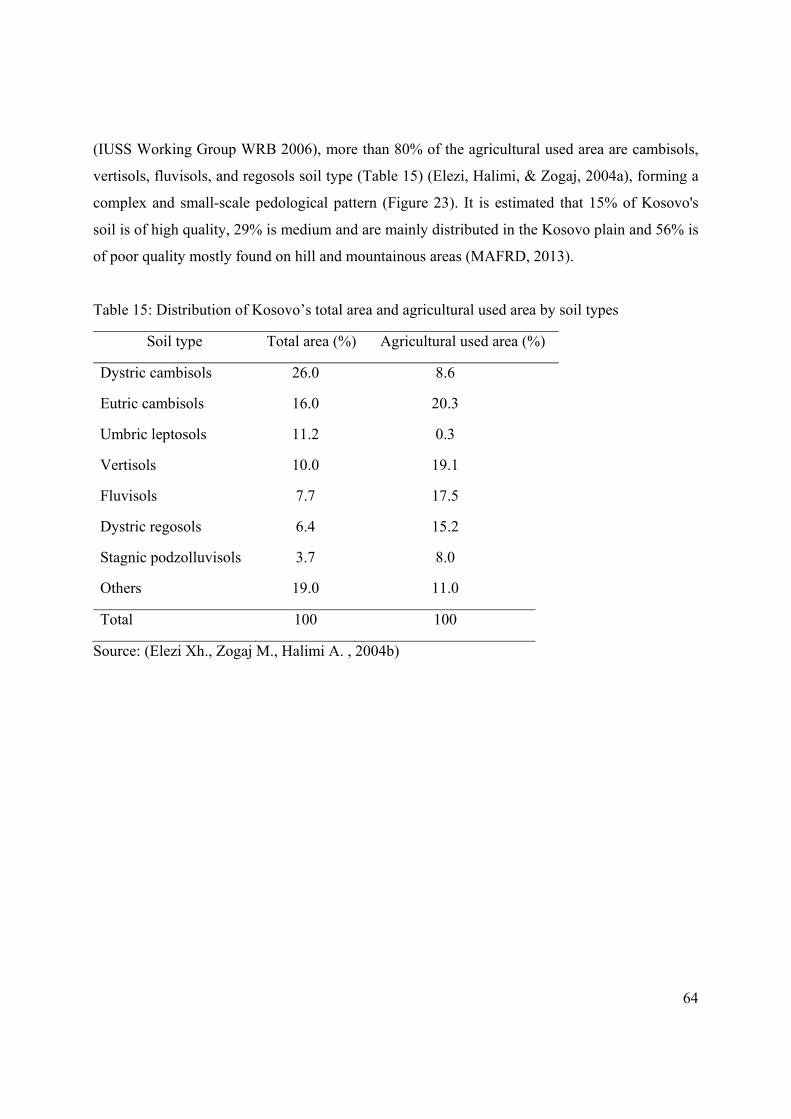
64

(IUSS Working Group WRB 2006), more than 80% of the agricultural used area are cambisols,

vertisols, fluvisols, and regosols soil type (Table 15) (Elezi, Halimi, & Zogaj, 2004a), forming a

complex and small-scale pedological pattern (Figure 23). It is estimated that 15% of Kosovo's

soil is of high quality, 29% is medium and are mainly distributed in the Kosovo plain and 56% is

of poor quality mostly found on hill and mountainous areas (MAFRD, 2013).

Table 15: Distribution of Kosovo’s total area and agricultural used area by soil types

Soil type Total area (%) Agricultural used area (%)

Dystric cambisols 26.0 8.6

Eutric cambisols 16.0 20.3

Umbric leptosols 11.2 0.3

Vertisols 10.0 19.1

Fluvisols 7.7 17.5

Dystric regosols 6.4 15.2

Stagnic podzolluvisols 3.7 8.0

Others 19.0 11.0

Total 100 100

Source: (Elezi Xh., Zogaj M., Halimi A. , 2004b)

65

Figure 23: Pedological map of Kosovo

Source: (Elezi, Halimi, & Zogaj, 2004a)

The study was carried out in three regions Prizren, Gjilan and Pejë, respectively at eight different

municipalities (Mamushë, Suharekë, Ferizaj, Rahovecë, Istog, Klinë, Viti, Ferizaj, Shtime.

4.1 Datacollection,samplingprocedureandtheanalysisperformed

The data set used in this study is entirely primary data and consists of two parts: (a) the data

covering information on household and farm characteristics and (b) the data associated with agri-

environmental issues, particularly with soil quality on the farm and the ecological aspect of

biodiversity generated by farms. Different data collection approaches were needed for each

objective stated in the study. The designed research for the study was conducted in three stages:

First stage: Preparing and conducting a survey with farmers

66

In the first phase of the study a survey was conducted with horticultural farms where tomato is

the main crop, intensively cultivated in greenhouses (cold poly-tunnels), grape-growing farms,

and apple farms. A structured questionnaire (Annex 2) was developed and used as an instrument

for data collection and it covered information on household and farm characteristics. The head of

the family members which in most of the cases was also the manager of the farm was included in

the interviewing process. The designed questionnaire comprised of five different sections and

within each section different questions were asked and measured on continuous, dichotomous,

multiple choice, open ended and rank order scale. The selection of the farms was performed

based on the registered farm list provided by the MAFRD. The farms were randomly selected

from the farm list. Initially, the total sample size comprised of 120 farms, which was equally

distributed for each selected crop in the study (40 per each crop). Later, in the phase of data

processing and analysis, 106 farms remained in the data set (38 tomato, 34 apple and 34 grape

farms) and 14 were removed due to either weak information provided by the farmers or detected

as outlier observation in the data set.

67

Table 16: Information on the data obtained through the survey and the analysis performed

Section Data Analysis Software used

1: Demographics

data on composition

of the farm

household

Age, education and

profession of the farm

household head and

other family members;

household size; and the

duration in years living

in the same village.

Descriptive statistics;

Analysis of Variance

(ANOVA);

Chi-square test.

Statistical Package

for the Social

Sciences (SPSS),

version 21

2: Employment

status, sources and

composition of the

income

Number of the

household members

employed in and out of

the farmstead; number of

the household members

working out of the

country;

composition and the

sources of income.


ANOVA;

Chi-square test;

Correlation.

SPSS version 21

3: Farm and land

use

Experience in farming;

reasons getting involved

in farming activities;

farmer’s satisfaction

with farming activities;

cultivated land in ha

(owned and leased land);

number of land parcels,

and farmer’s interest to

cultivate more land.


ANOVA;

Chi-square test;

Correlation.

SPSS version 21

4: Crop production Number of cultivated

crops; land allocated to

each cultivated crop.


SPSS version 21.

68

5: Yields, inputs

used in the

production process,

costs and gross

revenue.

Yields for considered

crops in the study;

quantity of inputs used

such as seeds/seedlings,

fertilizers, pesticides,

packaging, fuel, labor,

machinery.


efficiency analysis

including technical,

scale, cost, revenue

and allocative

efficiency;

truncated regression

analysis.

SPSS version 21

for descriptive

statistics;

Performance

Improvement

Management

Software (PIM-

DEA V3) for

efficiency analysis;

Eviews version 9

for truncated

regression analysis.

To ensure that the content of the developed questionnaire covers all information needed to

address the study objectives and it is functioning well in general, the validity of the instrument

was conducted using experts and field test.

69

Figure 24: Location of the sampled tomato farms

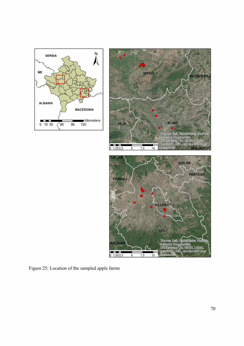
70

Figure 25: Location of the sampled apple farms

71

Figure 26: Location of the sampled grape farms

Second stage: Soil sampling and soil analysis

In the second stage of the study, soil samples were collected for each considered crop in the

study. In order to avoid the fall of sampling points in a straight line and to ensure that the entire

plot is represented, a grid pattern was applied as a scheme as it is shown in the Figure 27.

Figure 27: Scheme of the soil sampling

72

Soil samples for all selected crops where taken in a depth of 35cm from the surface, which

essentially represents the root zone where the plant can absorb soil nutrients. For the tomato

farms at each cold-poly tunnel with the dimension of 3*10m, five soil samples were collected

and merged as a composite sample per one cold-poly tunnel. The total number of cold poly-

tunnels at tomato farms was varying between 3 minimum to a maximum of 18, depending on the

farm size. Out of the total number of tunnels per farm, 2-3 tunnels were randomly selected and

included in the soil sampling procedure and the chemical soil valuation. Thus, in the end of the

process 2-3 replicates were obtained per each farm. In addition, five soil samples at the same

depth (35cm) were collected from uncultivated agricultural land situated near each farm and later

pooled as one composite sample representing uncultivated soil. For perennial trees (apple and

grape), replicates of the soil samples varied according to the orchard size. Similar to the tomato

farms, a grid pattern of the soil sampling was applied. In addition, a composite sample from five

soil samples representing uncultivated soils near each orchard (apple and grape) was collected. In

total (including replicates) 304 soil samples were attained for soil quality valuation.

Figure 28: Distribution of the total soil samples among farms in cultivated and uncultivated land

Laboratory chemical analysis were carried out in order to be able to describe internal soil

nutrition. Collected data based on laboratory chemical measurements were further aggregated

Total soil sampes n=340

Total soil samples at tomato farms

n=164

Cultivated land

n=124

Uncultivated land

n=40

Total soil samples at apple farms

n=80

Cultivated land

n=40

Uncultivated land

n=40

Total soil samples at grape farms

n=96

Cultivated land

n=56

Uncultivated land

n=40

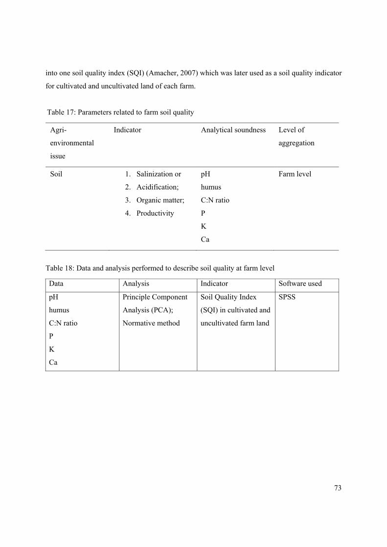
73

into one soil quality index (SQI) (Amacher, 2007) which was later used as a soil quality indicator

for cultivated and uncultivated land of each farm.

Table 17: Parameters related to farm soil quality

Agri-

environmental

issue

Indicator Analytical soundness Level of

aggregation

Soil 1. Salinization or

2. Acidification;

3. Organic matter;

4. Productivity

pH

humus

C:N ratio

P

K

Ca

Farm level

Table 18: Data and analysis performed to describe soil quality at farm level

Data Analysis Indicator Software used

pH

humus

C:N ratio

P

K

Ca

Principle Component

Analysis (PCA);

Normative method

Soil Quality Index

(SQI) in cultivated and

uncultivated farm land

SPSS

74

Third stage: Assessing ecological aspect of biodiversity provided by farm

In the third stage of the research, data associated with the habitat quality of cultivated farm land

was collected and considered as an indicator of the ecological aspect of biodiversity provided by

on-farm management practices.

Table 19: Data and analysis performed to assess agri-biodiversity provided by farms

Agri-

environmental

issue

Indicator Analytical soundness Level of

aggregation

Biodiversity 1. Number of

cultivated

varieties within a

crop

2. Ecological aspect

of biodiversity

Shannon’s Diversity

Index (SHDI)

% of open soil

% of annual species

% of perennial species

% of grasses

% of herbs

Farm level

4.2 Descriptiveanalysis

The first part of the results provide figures and analysis of the data set obtained from 1021 family

farms. Descriptive statistics, Analysis of Variance (ANOVA) and Chi-square test is used to

describe and relates the main household characteristics age, household size, and education with

other socio-economic factors. The next section proceeds with farm characteristics, land use, and

crop production.

1 8 farms were excluded from the data analysis due to missing data.

75

4.2.1 Householdcharacteristics The overall household size is relatively large, with an average of 9.76 (Standard Deviation (SD)

= 5.29) family members per household. On average, the household size of the farms oriented in

tomato production is significantly (p < 0.001) larger than the farms oriented in apple and grape

production. Study results showed a very high degree of inequality in regard to gender of the farm

household head where, 99% of the farms were male-headed. All family farms (in total 102) were

living in the same village since the head of the family farm was born. The average age of the

farmers from the entire sample is 46.75 (SD = 11.11) years old. On average, farmers oriented in

tomato production were significantly (p < 0.05) younger and considerably less educated (p <

0.01) compared to the apple and grape producers. The number of tomato farmers having

additional profession aside from a farmer was different and significantly ( = 9.13, df = 2 p <

0.05) lower compared to the two other group of farms. The likelihood of having additional

profession aside from a farmer was statistically proven to be dependent on the farmer's education

level ( = 14.49, df = 2 p < 0.01). This result corresponds with the statistical test performed for

differences in terms of education, where tomato farmers were significantly less educated among

the three group of farms.

Table 20: Summary statistics of the farm household characteristics

Farm household characteristic Mean SD Min Max

HH size at tomato farms 12.16 6.18 4 26

HH size at grape farms 9.40 4.96 4 27

HH size at apple farms 7.23 2.67 3 14

HH size for entire farms 9.76 5.29 3 27

Farmer's age at tomato farms 43.11 7.51 31 65

Farmer's age at grape farms 48.40 13.44 25 84

Farmer's age at apple farms 49.30 11.01 30 72

Farmer's age for entire farms 46.75 11.11 25 84

Farmer's education at tomato farms 9.89 2.87 4 20

Farmer's education at grape farms 11.97 2.94 8 18

Farmer's education at apple farms 13.83 2.30 8 18

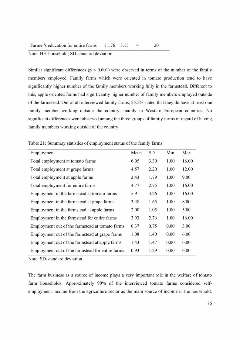
76

Farmer's education for entire farms 11.76 3.15 4 20

Note: HH-household; SD-standard deviation

Similar significant differences (p < 0.001) were observed in terms of the number of the family

members employed. Family farms which were oriented in tomato production tend to have

significantly higher number of the family members working fully in the farmstead. Different to

this, apple oriented farms had significantly higher number of family members employed outside

of the farmstead. Out of all interviewed family farms, 25.5% stated that they do have at least one

family member working outside the country, mainly in Western European countries. No

significant differences were observed among the three groups of family farms in regard of having

family members working outside of the country.

Table 21: Summary statistics of employment status of the family farms

Employment Mean SD Min Max

Total employment at tomato farms 6.05 3.30 1.00 16.00

Total employment at grape farms 4.57 2.20 1.00 12.00

Total employment at apple farms 3.43 1.79 1.00 9.00

Total employment for entire farms 4.77 2.75 1.00 16.00

Employment in the farmstead at tomato farms 5.91 3.26 1.00 16.00

Employment in the farmstead at grape farms 3.48 1.65 1.00 8.00

Employment in the farmstead at apple farms 2.00 1.05 1.00 5.00

Employment in the farmstead for entire farms 3.93 2.76 1.00 16.00

Employment out of the farmstead at tomato farms 0.37 0.75 0.00 3.00

Employment out of the farmstead at grape farms 1.08 1.40 0.00 6.00

Employment out of the farmstead at apple farms 1.43 1.47 0.00 6.00

Employment out of the farmstead for entire farms 0.93 1.29 0.00 6.00

Note: SD-standard deviation

The farm business as a source of income plays a very important role in the welfare of tomato

farm households. Approximately 90% of the interviewed tomato farms considered self-

employment income from the agriculture sector as the main source of income in the household.

77

Only 8.1% of the tomato family farms, income flows from self-employment excluding

agriculture and touristic sector was the main contribution of the household income. Grape family

farms choose to diversify more income sources in order to support living standards. In

comparison to the tomato farms, a smaller percentage (74%) of the grape family farms declared

that the generated income from agriculture activities is the main source of income for their

livelihood. A survey conducted in Albania reported that 60% of the farm household incomes

come from farming activity and 22% of the income derives from self-employment or waged

labor (Wehinger & Zhllima, 2013).

For other grape farms, wage income excluding agriculture and the tourist sector (14.3%), self-

employment income excluding agriculture and touristic activities (5.7%) and other income

sources like private and public transfers (5%) were considered to be the main source of income.

A completely different situation can be found for most of the apple producers where the farm

household wellbeing is mainly based on off-farm activities. Only 23.3 % of apple producers earn

income mainly from the agriculture activities. Majority (43.3%) make a living from wage

income and 33.3% from self-employment excluding agriculture and the tourist sector. For most

of the apple producers income from agriculture is an additional source of income with the

purpose to diversify and stabilize their household income.

Farm household income sources were further examined to see how the income pattern relates to

the other farm household characteristics. Study results did not show a significant association

between the sources of income and the age groups of farmers. Household size (all family

members dependent on the household financial support including students away at school), farm

size (all cultivated land including owned and leased land) were not shown to be significant

determinant factors for the household income sources. Farmer's education level and experience

in terms of the number of years active in farming were significantly correlated and the main

factors contributing to the income source determination of farm household. In terms of education

level, similar patterns were found in the study conducted by (Zezza, 2007) in cross comparison

of fifteen developing countries. Households with lower levels of education are likely to be more

engaged in on-farm activities and rely more on agriculture income. Study results from (Estudillo

& Otsuka, 2010) showed that secondary and tertiary education was positively corralled to non-

78

farm income. Another study conducted by (Miftari & Gjonbalaj, 2013) showed that the higher

the education level the higher probability that farm households will engage in non-farm

activities, having positive effect on household’s non-farm diversification as well as improved

household welfare.

Table 22: Correlation of the farm household income sources with farm characteristics

Farm household income sources

Farm characteristics Df p-value Cramer's V

Farmer's age 9.18 9 0.42 0.17

HH size 10.78 9 0.29 0.18

Farm size 9.00 6 0.17 0.29

Education 27.10 6 0.00 0.51

Experience 19.17 6 0.00 0.30

Note: HH size- household size.

Income of farm households and its contribution to the total household income varies according to

the farm typology and commodity. On average, tomato farms were having the highest share of

income from agriculture and compared to the two other groups of farms, the difference was

proved to be statistically significant (p < 0.001). For farmers oriented more on apple production

the average farm income contribution to the total household income was 55% (SD 30%). The

level of income earned from non-agricultural activities (mainly as wage or self-employment

income) was considerably higher for apple farm households. The average contribution of farm

income to the total income was slightly higher for grape producers 58% (SD 28%). However, for

tomato producers, farm income was the main contributor to the total household income with 83%

and the level of income from agriculture activities was significantly higher compared to grape

and apple farms (p < 0.05). Another part of income for tomato farms was mostly coming from

private (remittances) or public (pensions) transfers. The composition of human and natural assets

at farm household was a key determinant for the income level. The household size, number of

family members working actively on farm and farm size, were all positively and significantly

associated with the farm income. The Person's correlation coefficient of household size and

79

income was r = 0.198, p < 0.05, for employment r = 0.207, p < 0.05 and farm size r = 0.496 p <

0.001. No significant correlations were observed between farmer's age, education, and

experience in agriculture with the total income of farm household.

Table 23: Annual income of farm households by source of income

Source of income Mean SD Min Max

Total income at tomato farms 19,322 11,467 5,580 71,680

Total income at grape farms 21,883 20,112 3,600 92,000

Total income at apple farms 21,121 14,722 3,500 70,000

Total income for entire farms 20,730 15,700 3,500 92,000

Income from agriculture at tomato farms 14,456 6,466 725 30,000

Income from agriculture at grape farms 10,366 9,142 1,200 40,000

Income from agriculture at apple farms 9,494 7,978 1,000 35,000

Income from agriculture for entire farms 11,593 8,133 725 40,000

Income from non-agricultural activities at grape farms 6,310 2,569 2,400 14,400

Income from non-agricultural activities at apple farms 12,976 8,447 1,500 40,000

Note: Descriptive statistics of the income from non-agricultural activities for tomato farms were

not reported as only 5 household farms out of 37 were generating income from non-agricultural

activities.

4.2.2 Farmcharacteristics

The average size (in terms of physical measure-the number of hectares) of an apple farm was

6.32 ha (SD = 5.10). About 25% of the total apple farms were smaller than 3 ha and 75% lay

below 7.25 ha. The ANOVA test showed that on average, apple farms were significantly bigger

compared to the grape and tomato farms (p < 0.05). The average size of grape farms was 4.13 ha

(SD = 3.33), which is significantly smaller than apple farms but bigger than tomato farms with

3.30 ha (SD = 1.92). The size of tomato farms was ranging from 0.5 up to 8 ha.

Most of the farms are considered to be well established farms, as on average they were active in

farming for 28.46 years (SD = 15.57). The smallest mean of farming experience was for apple

80

producers 18.90 years (SD = 15.47), followed by tomato producers 28.53 years (SD = 12.57) and

the grape producers 36.57 (SD = 14.63). The mean of farming experience has been proven to be

statistically different among the three groups of farms (p < 0.001). No significant relationship

was observed between farming experience and farm size. The table 24 presents the distribution

of total farms by farming experience.

Table 24: Distribution of the farms by farming experience

Farming experience in years 1-10 < 10 -20 < 20-30 < 30

Frequency in % 20.6 11.8 27.5 40.2

The main reason for getting engaged in agriculture activities was differing among the three

groups of farms. A majority (63%) of the grape producers stated that "tradition" is the main

reason they got involved into farming. About 33% of the apple producers stated that "income

generation" is the only reason they were engaged in farming activities and an approximately

equal percentage (32%) of grape producers gave the same answer. The main stated reason

differed for tomato producers, where 43% declared that "no other opportunity" was the main

reason getting involved in farming activities and just about 22% because of income generation.

A smaller number out of the interviewed farmers stated other reasons, e.g. "because of hobby".

The stated reason of getting engaged to farming was significantly different among farmers

grouped by education level ( = 15.27, DF = 4, p < 0.01) and farming experience ( = 15.82,

DF = 8, p < 0.05). Whereas, farmers with primary education were involved in agriculture mainly

because of income generation or as there was no other opportunity for them, for those with

secondary and tertiary education "tradition" was the most affirmed reason. No statistically

significant dependency was examined between the farm size and farmer's age with the stated

reason of getting involved into farming activities. Figure 29 presents the satisfied level of

farmers in farming activities. The satisfaction level was proclaimed in the scale of 1-not satisfied

at all to 5-very satisfied.

81

Figure 29: Satisfied level of farmers in farming activities

4.2.3 Landuseandsoilquality The proportion of tomato farmers leasing land from other landowners was 59.5%. This

proportion was approximately the same for grape (20%) and apple farms (23.3%). The main

reason of leasing land for agriculture purposes is that this was the easiest way for farmers to

expand their agriculture business without high capital investment costs like buying additional

land. The rental price was varying from region to region and it was dependent on many different

factors like location, soil type, productivity and water availability. The minimum to maximum

annual price paid for leasing land was 100 to 200 EUR per ha. The price was significantly higher

in Mamusha region (500-1000 EUR per ha) as in the surrounding area where most of the tomato

farms were located, there is no much land available for renting, due to its intensive use for

vegetable production. For the entire sample, the farm land is considered to be very fragmented

and scattered over a wide area. There was no significant difference in the possession of land

plots between the three groups of farms (p > 0.05). The overall mean of the land plots was 5.47

(SD =2.87), where 25% of the total farms were having less than 4 land plots and 75% up to 7

plots. The number of land plots in the farm was positively and significantly correlated to the

farm size (r = 0.42, p < 0.001).

0

10

20

30

40

501

2

34

5

Apple farms Grape farms Tomato farms

82

4.2.4 Assessmentofsoilquality

Soil is considered to be a crucial component not only for producing food and fibers, but also for

maintaining local, regional and global environmental quality (Glanz AA., 1995). In addition to

the food and fiber production, high quality soil plays a key role in stabilizing natural ecosystems

and improving air and water quality (Gregorich E., 1993). There is a high level of interaction

between the environment and the production and therefore proper agricultural land management

practices improve the quality of soils and other environmental goods (Cooper T., 2009). The

level of soil quality is evaluated based on several indicators which include the proportion of

organic matter, its vulnerability by wind and water, structure and capacity for infiltration the

health of its biota and the level of contamination (SoCo, 2009). The soil quality concept is

considered to be a helpful tool in assessing the impact of land use and soil/crop management

practices on biological, chemical and physical components of the soil (Masto R.E., 2008).

Reduction in the crop yield is often attributed to land degradation caused by various factors and

one of them is also inability of small-scale farmers to adopt technologies that improve soil

fertility and conservation (Mbaga-Zemgawale Z., and Folmer H., 2000). Soil chemical

parameters were also shown to be significant determinants for floristic composition-

phytodiversity (Wellstein C., Otte A., and Waldhardt R., 2007). Soil quality variations at farm

level may be attributed from two possible sources: 1) natural differences in soil properties, and

farm-made differences due to the different farm practices such as fertilizers application, soil

conservation techniques etc. (Masterson T., 2007). Therefore, it is important that farmers get

motivated to follow farming practices to maintain and manage natural resources such as soil

(Cooper T., 2009). Cross compliance as a horizontal tool for pillar I and II plays a crucial role in

protection, conservation and improvement of soil (SoCo, 2009).

In our study, the soil quality assessment at the farm level refers mainly to the chemical

parameters. Several studies have shown that soil quality significantly determines technical

efficiency of agriculture (Nowak A., 2015). Nowak A., et al (2015) regressed soil productivity

index as independent variable and found out that variation on technical efficiency at farm level

was significanlty determined by soil productivity index. A study conducted by Karimov A.

(2013) showed that farmers with higher soil fertility index were attaining higher technical

83

efficiency scores, and suggests that further actions are needed towards preserving the soil quality

and improvement of land tenure system (Karimov A., 2013). Overall technical efficiency of

sugar cane farmers in Central Negors was positivelly related to soil type (Padilla-Fernandez M.

D., and Nuthall L. P., 2009). Statistically significant difference was also observed in the means

of soil quality indices between the farmers obtaining higher technical efficiency scores compared

to those defined as technically inefficient (Kelly E., 2012). It is understandable that farmers with

poor soil quality may attempt to increase yields through additional use of inputs e.g. fertilizers

and pesticides and as result achieve lower technical efficiency scores.

The Soil Quality Index (SQI) for each production system for cultivated and uncultivated land

was calculated using two different methods:

1. Principle Component Analysis (PCA), and

2. Normative approach (NA).

Chemical soil parameters used in SQI valuation: Total nitrogen (Nt) and total carbon (Ct) levels

were assessed using a CN-analyzer; the AL-method described by (Egner, Riehm, & Domingo,

1960) was used in estimating levels of plant available phosphorus (PALM) and potassium (KALM);

pH values were determined in water (1:2.5, soil water ratio) and CaCl2; The Weight Loss on

Ignition method was used for measuring organic matter in the soil.

The obtained laboratory values of soil chemical parameters were aggregated into one index

value.

84

Figure 30: A generalized framework for developing soil quality indices (from Karlen et al. 2001)

1. Soil quality estimation using PCA approach: in the first phase the values of thresholds

presented in the table 26, chemical soil parameter values were altered into unit less scores (0-1).

A Linear scoring function (LSF) as presented below was used to calculate the scores for each soil

property value (Masto R. E., 2008). In the case when soil chemical parameter was considered to

be as 'more is better' the following LSF was used:

(6)

LSF (LS) = (SPV – LTV) / (UTV – LTV)

whereas, in the case when soil chemical parameter was considered to be as 'less is better' the

following LSF was used:

(7)

(LS) = 1 – (SPV – LTV) / (UTV – LTV),

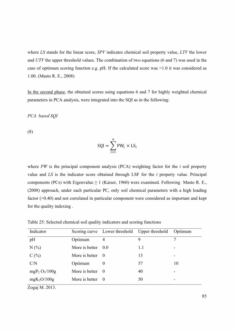
85

where LS stands for the linear score, SPV indicates chemical soil property value, LTV the lower

and UTV the upper threshold values. The combination of two equations (6 and 7) was used in the

case of optimum scoring function e.g. pH. If the calculated score was >1.0 it was considered as

1.00. (Masto R. E., 2008)

In the second phase, the obtained scores using equations 6 and 7 for highly weighted chemical

parameters in PCA analysis, were integrated into the SQI as in the following:

PCA based SQI

(8)

SQI PW LS

where PW is the principal component analysis (PCA) weighting factor for the i soil property

value and LS is the indicator score obtained through LSF for the i property value. Principal

components (PCs) with Eigenvalue ≥ 1 (Kaiser, 1960) were examined. Following Masto R. E.,

(2008) approach, under each particular PC, only soil chemical parameters with a high loading

factor (>0.40) and not correlated in particular component were considered as important and kept

for the quality indexing .

Table 25: Selected chemical soil quality indicators and scoring functions

Indicator Scoring curve Lower threshold Upper threshold Optimum

pH Optimum 4 9 7

N (%) More is better 0.0 1.1 -

C (%) More is better 0 13 -

C/N Optimum 0 57 10

mgP2 O5/100g More is better 0 40 -

mgK2O/100g More is better 0 50 -

Zogaj M. 2013.

86

PCA results for cultivated land at tomato farms

Figure 31: PCA scree plot of soil chemical parameters in cultivated land at tomato farms

Table 26: Pattern matrix of soil chemical parameters in cultivated land at tomato farms

Soil chemical parameter Component

1 2 3

C total % .961 .094 .096

C/N % .887 -.217 -.279

N total % .745 .286 .309

mgP2O5/100g -.131 .904 -.151

mgK2O/100g .159 .779 .047

pH (H2O) -.026 -.121 .975

Note: SPSS software has been used to perform PCA analysis.

87

Bold and underlined soil chemical parameters in components 1, 2 and 3 were showing high

loading factor (>0.40) and before considering for the soil quality indexing, a correlation matrix

was performed as presented in the table 27.

Table 27: Correlation matrix of the soil chemical parameters in cultivated land at tomato farms

N total

%

C total

%

C/N % mgP2O5/100g mgK2O/

100g

pH(H2O)

N total %

Pearson

Correlation

1 .896** .364* .219 .346* .244

Sig. (2-tailed) .000 .023 .181 .031 .134

C total %

Pearson

Correlation

.896** 1 .726** .059 .296 .117

Sig. (2-tailed) .000 .000 .722 .067 .480

C/N %

Pearson

Correlation

.364* .726** 1 -.153 .080 -.119

Sig. (2-tailed) .023 .000 .353 .629 .470

mgP2O5/

100g

Pearson

Correlation

.219 .059 -.153 1 .452** -.106

Sig. (2-tailed) .181 .722 .353 .004 .519

mgK2O/

100g

Pearson

Correlation

.346* .296 .080 .452** 1 .061

Sig. (2-tailed) .031 .067 .629 .004 .710

pH(H2O)

Pearson

Correlation

.244 .117 -.119 -.106 .061 1

Sig. (2-tailed) .134 .480 .470 .519 .710

**. Correlation is significant at the 0.01 level (2-tailed). *. Correlation is significant at the 0.05 level (2-tailed).

In the first component C total (%), C/N (%) and N total (%) were the highest loading factors, but

in the correlation matrix (Table 27) we can observe that C total (%) was statistically significantly

correlated with C/N (%) and N total (%). Therefore, only C total (%) from the first component

88

was considered in soil quality indexing. In the second component mgP2O5/100g and

mgK2O/100g were highly weighted factors, however the Pearson's correlation coefficient

between this two variables was statistically significant and therefore only mgP2O5/100g was

considered in indexing. In the third component only pH was highly weighted and included in the

index calculation.

Table 28: Calculation of the soil quality index at tomato farms

SQII SQII = (PWICtotal % * LSI Ctotal %) + (PWImgP2O5/100g * LSI mgP2O5/100g) + (PWIpH* LSIpH)

SQII = (0.961*0.090) + (0.904*0.658) + (0.975*0.380) = 1.053

SQII was normalized to get the maximum value of 1 as in the following formula:

NSQII = ƩSQII/ƩLSI; NSQII = 1.053/1.130 = 0.932

SQIO SQIO = (PWOCtotal % * LSO Ctotal %) + (PWOC/N %* LSOC/N %) + (PWOpH* LSOpH) +

(PWOmgK2O/100g * LSOmgK2O/100g)

SQIO = (0.965*0.075) + (0.843*0.116) + (0.885*0.342) + (0.623*0.155) = 0.570

NSQIO = ƩSQO/ƩLS; NSQII = 0.570/0.689 = 0.827

Note: SQII stands for soil quality index in cultivated land; SQIO is soil quality index in

uncultivated land; NSQI indicates normalized soil quality index; PWI is PCA weighting factor

for soil chemical parameters in cultivated land; PWO is PCA weighting factor for soil chemical

parameters in uncultivated land; LSI stand for linear scoring in cultivated land and LSO for

linear scoring in uncultivated land. Same calculation was performed for apple and grape farms.

As it can be seen from the calculations (table 28) the soil quality index in cultivated and

uncultivated land was composed of different soil chemical parameters. Therefore, it was not

considered an appropriate approach to be compared for the differences between the SQII and

SQIO. As a result, a normative approach was considered as presented in the following formula.

89

2. Soil quality estimation using normative approach:

The individual index values for all chemical soil parameters were summed to give a total SQI:

Total SQI = Ʃ individual soil property index values

The maximum value that SQI could take was 12, which is calculated based on the six chemical

parameters measured. The total SQI is then expressed as a percentage of the maximum possible

value of the total SQI for the soil parameters measured (Amacher M. C., 2007).

( 9)

%

∗ 100

90

Table 29: Soil quality index values and soil parameter threshold values and interpretations

Parameter Level Interpretation Index

mgP2O5/100g 0 up to 10 Low-possible deficiencies 0

> 10 up to 20 Moderate-adequate levels 1

> 20 High-excellent reserve 2

mgK2O/100g 0 up to 10 Low-possible deficiencies 0

> 10 up to 20 Moderate-adequate levels 1


mgCa/100g up to 20 Low-possible deficiencies 0

>20 up to 400 Moderate-adequate levels 1


C% total >0-1 Very low 0

>1-2 Low-possible deficiencies 1

>2-3 Moderate-adequate levels 2

>3-13 High-excellent reserve 2

N% total >0-0.1 Very low 0

>0.1-0.2 Low-possible deficiencies 1

>0.2-0.3 Moderate-adequate levels 2

>0.3-1.1 High-excellent reserve 2

pH 3.1-4.0 Strongly acid 0

4.01-5.5 Moderately acid 1

5.51-6.8 Slightly acid 2

6.81-7.2 Near neutral 2

7.21-7.5 Slightly alkaline 1

7.51-8.5 Moderately alkaline 1

>8.5 Strongly alkaline 0

Source: (Amacher M. C., 2007).

91

4.2.5 Resultsofthesoilqualityindexunderthreedifferentproductionsystems

As the SQI was calculated for cultivated and uncultivated lands in three production systems, we

distinguished SQI into SQII, standing for cultivated land, and SQIO for uncultivated land. The

average SQIIPCA for tomato farms was estimated to be 0.80 (SD = 0.18) with a range from

minimum 0.32 to maximum 0.95. The SQIOPCS was slightly smaller than SQIIPCA with an

average of 0.75 (SD = 0.04), a minimum of 0.64 and maximum of 0.84. Different SQI results

were obtained with a normative approach (Table 30).

Table 30: The SQII and SQIO of tomato farms using normative approach

SQI Mean SD Minimum Maximum

SQIINA 0.63 0.12 0.33 0.92

SQIONA 0.57 0.13 0.33 0.83

Note: Subscript NA stands for normative approach.

Figure 32: Comparison of the estimated SQI for cultivated and uncultivated land of tomato farms

using a normative approach

The average SQIIPCA for grape farms was estimated to be 0.970 (SD = 0.05) with a range from

minimum 0.619 to maximum 0.987. The SQIOPCS was slightly smaller than SQIIPCA with an

0

0.1

0.2

0.3

0.4

0.5

0.6

0.7

0.8

0.9

1

1 3 5 7 9 11 13 15 17 19 21 23 25 27 29 31 33 35 37

SQII SQIO

92

average of 0.937 (SD = 0.08), a minimum of 0.544 and maximum 0.975. The table below present

results for the SQI of grape farms obtained using a normative approach.

Table 31: The SQII and SQIO of grape farms using a normative approach


SQIINA 0.46 0.16 0.16 0.83

SQIONA 0.41 0.14 0.08 0.66

Note: Subscript NA stands for normative approach.

93

Figure 33: Comparison of the estimated SQI for cultivated and uncultivated land of grape farms


Table 32: The SQII and SQIO of apple farms using principle component analysis and a normative approach


SQIIPCA 0.62 0.03 0.50 0.71

SQIINA 0.62 0.11 0.33 0.83

SQIOPCA 0.70 0.11 0.18 0.79

SQIONA 0.62 0.13 0.33 0.91

Note: Subscript PCA stands for principle component analysis, NA-normative approach.

0

0.1

0.2

0.3

0.4

0.5

0.6

0.7

0.8

0.9

1 2 3 4 5 6 7 8 9 10111213141516171819202122232425262728293031323334

SQII SQIO

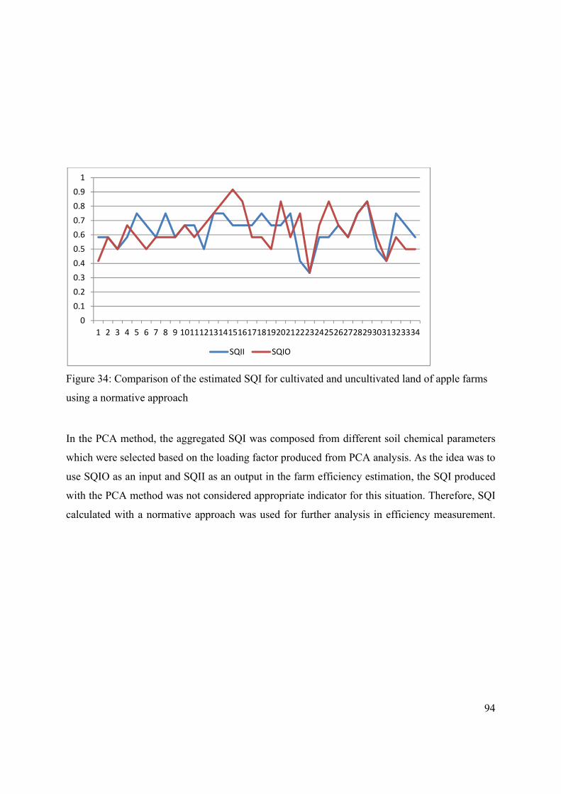
94

Figure 34: Comparison of the estimated SQI for cultivated and uncultivated land of apple farms


In the PCA method, the aggregated SQI was composed from different soil chemical parameters

which were selected based on the loading factor produced from PCA analysis. As the idea was to

use SQIO as an input and SQII as an output in the farm efficiency estimation, the SQI produced

with the PCA method was not considered appropriate indicator for this situation. Therefore, SQI

calculated with a normative approach was used for further analysis in efficiency measurement.

0

0.1

0.2

0.3

0.4

0.5

0.6

0.7

0.8

0.9

1

1 2 3 4 5 6 7 8 9 10111213141516171819202122232425262728293031323334

SQII SQIO

95

4.3 Biodiversitydefinitionanditsimportance

A considerable number of studies highlight that the term “biological diversity” came into

prominence in the early 1980s. Magurran (2004) relates its earliest reference to Gerbilskii and

Petrunkevich (1955, p.86) who used this term in the context of intraspecific variation in the

behavior and life history (Magurran A. , 2004). Haper and Hawksworth (1995) date its first use

back to the 80s when Lovejoy used it to indicate the number of species present and to Norse et

al. (1986), who firstly dissected biological diversity into three levels: genetic (within species),

species (species numbers) and ecological (community) diversity (Aswathanarayana, 2012). The

biodiversity concept is widely used; (Callicot, 1999) distinguishes it between compositionalism

which is based on a biological hierarchy of organisms in species populations interacting in biotic

communities and functionalism which is based on thermodynamic energy flows and nutrient

cycles and the ontology of processes and functions. The United Nations Conventions on

Biological Diversity defines it as:

'the variability among organisms from all sources, including inter allia, terrestrial, marine

and other aquatic ecosystems and the ecological complexes of each they are part; these include

diversity within species, between species, and of ecosystems' (UNEP, 1992).

This involves three main hierarchical levels of biodiversity (Lévéque C., & Mounolou J. C.,

2003):

Diversity within species: variation of genes within species

Diversity between species: diversity of various species i.e species richness

Diversity of ecosystems: variations of the habitats and ecological niches from region to global scale

96

According to (Wilson, 1988) definition it is 'the variety of life at every hierarchical level and

spatial scale of biological organizations: genes within populations, populations within species,

species within communities, communities within landscapes, landscapes within biomes, biomes

within biosphere'. Biodiversity also refers to the totality of the species across the full range of

terrestrial organisms (i.e. invertebrate animals, protists, bacteria and fungi, above and below

ground and vertebrates and plants which constitute the main concerns of biodiversity

conservation (Swift M.J, 2004).

Taking into consideration that biological diversity implies different levels, from genes to species

to ecosystems, the value of biodiversity can be defined in a number of different ways (Waldhardt

R., and Otte A. , 2003). A hierarchical characterization of biodiversity that identifies the major

components at several levels, provides a useful conceptual framework to assess the overall status

of biodiversity (Noss F. R. , 1990). 'The hierarchical concept recognizes that the effects of

environmental stresses will be expressed in different ways at different levels of biological

organization and the effects at one level can be expected to reverberate through other levels

(Noss F. R. , 1990).' According to Noss (1990), habitat variables presented in the scheme (Annex

1) were assumed to be important to the species and it obviates the need to monitor the

populations. However, habitat valuation data was not further used in the environmental

efficiency estimation.

The most important functions that biodiversity can provide to humankind can be grouped into

utilitarian also called direct use, indirect and intrinsic known also as non-use values using total

economic value framework (Brander L., 2010). Direct use value is mainly derived from goods

that can be extracted, consumed and enjoyed directly, whereas indirect, also known as a non-

extractive use value, is mainly derived from the services the environment provides (Dixon J.,

Pagiola S., 1998). Non-use or intrinsic values include existence value, which ensures the survival

of biological sources (Pearce R. K., Turner D. W., 1990) and relates to human cultural, social

and ethical values (Swift M.J, 2004). Biodiversity contributes to ecosystem life support functions

and the preservation of ecological structure and integrity, which is the functional value of

97

diversity, recognized lately in the economic literature (Kerry-Turner, 2004). Biodiversity

performs fundamental life-support services without which human civilization would cease to

thrive (Daily G. C. & et al, 1997).

(Vandermeer J., 1998) defines the role of biodiversity in agro-ecosystems and links between

diversity and function in three main hypotheses: 1) Biodiversity enhances ecosystem function

because different species perform different functions and thus redundancy is built into the

system; 2) Biodiversity is neutral or negative as there are more species compared to functions; 3)

Biodiversity enhances ecosystem function as those components appearing redundant at one point

in time become important when environmental changes occur.

In agriculture systems, land use changes and agriculture intensification through specialization in

one or few productive plant or animal species of value to humans often reduces diversity to

genetically homogenous species. In systems (Swift, 1996) distinguishes planned diversity,

implying the plants and livestock are purposely retained and managed by the farmer and

associated diversity related to the composition of planned diversity which influences the nature

of the associated biota like plants animal microbes.

Biodiversity is usually higher on farmland that is managed at low intensity (Beaufoy G., 2007).

Landscapes rich in biodiversity are in benefit also for soil conservation, which is being lost

mainly due to the intensive farming practices (Beaufoy G., 2007). In Europe, starting from the

early 1990s it has been acknowledged that maintain of low intensive farming practices that co-

creates landscapes and biotopes is important for biodiversity conservation (O'Rourke E. and

Kramm N., 2012). The relatively new concept known as High Nature Value (HNV) farming

systems have a tendency to yield lower incomes from the market and receive income payments

from CAP 'Pillar 1' (O'Rourke E. and Kramm N., 2012). The aim of this concept is to distinguish

extensive farming systems to intensive farming systems that degrade nature (Solovyeva I. and

Nuppenau A. E., 2013) and to link ecology, farming and public policies components and

management practices that promote HNV farming systems (Beaufoy G., 2007). Furthermore, the

98

HNV farming concept supports a holistic system of extensive land use practices including the

connectivity between farming and nature (Solovyeva I., and Nuppenau E. A., 2012).

The biodiversity as a multifunctional use of an ecosystem is economically valuable to

communities and to society as whole and therefore is of high importance (Balmford A., 2002).

Valuation of biodiversity and its recognition as a good that society esteems ensures better

balance in the decision-making and orientation of policy makers concerning biodiversity use and

its management. Impact assessment in a decision making system and management utilizing

trade-off analysis is essential for the sensible use of ecosystem sources (Müller F., 2010).

4.4 Measurementofbiodiversity The quantitative measurement of biodiversity is considered to be essential in understanding how

biodiversity contributes to ecosystem functioning, enhances human well-being and the services

that are being lost when biodiversity declines. The two main classes, ecological and economic,

traditionally employed different concepts for biodiversity measurement. Ecologists weight

species according to the relative abundance, while economists argue that in diversity

measurement, different species should be weighted differently according to the attributes they

possess (Baumgärter, 2005). No single unified approach and measure of biodiversity exists.

Therefore it is difficult and quite challenging to identify proper indicators. Ecologists employ

different concepts in regard to this measure, like species richness, Shannon-Wiener-entropy,

Simpson's index, and the Berger-Parker index, economists in general employ pairwise-

dissimilarity between species or weighted attributes of species.

In agricultural systems, intensification and specialization derived by market demands and land

use changes and often influenced by subsidies are considered to be influencing factors of the

biodiversity loss. In this regard, does the divergence between those who influence the provision

of services and those who benefit from this services bring up the issue of externality? Farming

activities may provide positive or negative effects which markets failed to internalize and

99

therefore farmers do not pay or get compensated in the case of negative or positive provisions.

Ecologists have quantified the species level of biodiversity in two ways: richness - the number of

species in a given area and evenness - how evenly balanced are the abundances of each species,

where the abundance of species is the number of individuals present (Armsworth P. R., 2004). A

considerable number of environmental economic studies have quantified evenness and richness

of diversity using the Shannon-Weiner diversity index (SHDI) e.g. (Pacini C., 2003) (Miettinen,

2004) (Di Falco S., and Perrings C., 2005) (Sipiläinen T., 2008) (Sipiläinen T., and Huhtala A.,

2011). In our economical production theory we use planned diversity, more specifically diversity

within species, as a positive by-product output in addition to yielding marketable outputs such as

in the tomato, grape and apple production.

The SHDI adapted from information theory measures both richness and evenness:

( 10)

∗ ,

Where S is the number of cultivated varieties within a given species, indicates the proportion

of the area covered by a specific variety within given species, and ln is the natural logarithm. The

index equals zero if the farmer is cultivating only one variety of a given species and it increases

with the number of cultivated varieties. The index reaches its maximum if the varieties are

cultivated in equal shares 1/ (McGarical K., Marks B. J., 1995). The obtained results of

the SHDI for each crop are presented the following graphical summary figures.

100

2.42.01.61.20.8

Median

Mean

1.901.851.801.751.701.651.60

1st Q uartile 1.5275M edian 1.75963rd Q uartile 1.9843M axim um 2.5038

1.6023 1.8639

1.6179 1.9290

0.3244 0.5148

A -S quared 0.63P -V alue 0.093

M ean 1.7331S tD ev 0.3979V ariance 0.1583S kew ness -0.592193K urtosis 0.277604N 38

M inim um 0.8468

A nderson-D arling N orm ality T est

95% C onfidence I nterv a l for M ean

95% C onfidence I nterv a l for M edian

95% C onfidence I nterv a l for S tD ev9 5 % C o nf id e nce I nte r v a ls

SHDI of tomato producers

Figure 35: SHDI graphical summary of tomato producers

Note: Minitab software was used to produce a graphical summary of SHDI.

2.01.61.20.80.4

Median

Mean

1.31.21.11.0

1st Q uartile 0.8461M edian 1.17663rd Q uartile 1.3709M aximum 2.0508

0.9599 1.2734

0.9649 1.2940

0.3623 0.5912


M ean 1.1167S tD ev 0.4492V ariance 0.2018S kew ness -0.231988Kurtosis -0.412041N 34

M inimum 0.2967

A nderson-D arling N ormality Test

95% C onfidence Interv al for M ean

95% C onfidence Interv al for M edian

95% C onfidence Interv al for S tD ev9 5 % C onfidence Inter v als

SHDI of grape producers

Figure 36: SHDI graphical summary of grape producers

101

2.01.61.20.8

Median

Mean

1.61.51.41.3

1st Q uartile 1.1976M edian 1.34343rd Q uartile 1.7192M aximum 2.0895

1.2560 1.5107

1.2828 1.5917

0.2944 0.4805


M ean 1.3834S tD ev 0.3650V ariance 0.1333S kew ness -0.308470Kurtosis -0.329748N 34

M inimum 0.5623

A nderson-D arling N ormality Test

95% C onfidence Interv al for M ean

95% C onfidence Interv al for M edian

95% C onfidence Interv al for S tD ev9 5 % C onfidence Inter v als

SHDI of apple producers

Figure 37: SHDI graphical summary of apple producers

The differences in the mean of SHDI between tomato, grape and apple producers were tested and

statistically significant differences at 5% level were observed among the three groups (F-statistic

= 21.01, p = 0.000). The SHDI of tomato producers was the highest among the three groups

followed by apple and grape producers. Due to many reasons, production systems under

perennial trees offer less possibilities to quickly change the compound and distribution of

varieties within a given species.

102

Apple producersGrape producersTomato producers

2.5

2.0

1.5

1.0

0.5

0.0

SHD

I

Figure 38: Box-plot of SHDI of tomato, grape and apple farms

103

5 ECONOMICEFFICIENCYANALYSIS Both input and output are relevant for evaluating the efficiency of DMU (Decision Making

Unit). This chapter presents the results of the efficiency measure including technical, cost,

revenue and allocative efficiency of the three different crops selected in the study. A set of linear

programs are presented and solved for all types of the efficiency estimations. Non-parametric

method DEA input and output oriented approaches were used to analyze the efficiency estimates

of the farms oriented towards tomato, grape and apple production. The obtained efficiency scores

from DEA analysis were further examined using truncated regression analysis to reveal the

relationships and determine how the variation of the efficiency scores can be explained by

factors describing farm characteristics.

5.1 Efficiencyestimation

5.1.1 Technicalefficiencyestimation Input oriented approach: Using the DEA input oriented model specification and assuming that

all farms are operating at an optimal scale, accounting for Constant Returns to Scale (CRS)

situation as defined by (Charnes A. C., 1978) and (Coelli T. P., 2005), the technical efficiency

scores for a given farm i is obtained by the following linear program (LP) problem:

( 11)

, ,

0,

0,

0,

104

where I farms with K inputs and M outputs, presented by the vectors xi - K x 1 vector of inputs of

the i-th farm; qi is a M x 1 vector of outputs of i-th farm; X is a K x I input matrix; Q is a M x I

output matrix; is a scalar and is an I x 1 vector of constraints.

The aim of the input oriented model is to minimize the input vector xi while satisfying at least the

given output levels. By virtue of the constraints, the optimal objective value of the scalar is at

most 1, meaning that the DMU is efficient if =1, otherwise the DMU is inefficient. The input

oriented model under CRS assumes that every increase in all inputs will result in a proportional

increase of the output. At CRS all farms are assumed to operate at an optimal scale. Results of

the Technical Efficiency (TE) measures under CRS specification will be confounded by Scale

Efficiency (SE), if not all farms are operating at an optimal scale. Therefore, calculation of the

TE scores under Variable Returns to Scale (VRS) assumption permits TE measures free of these

SE effects.

At VRS model as used by (Banker RD., 1984), additional constraint is added to the LP problem,

where N1' 1 replaces the constraint 0. This approach shapes a convex hull of

intersecting facets which envelops data more tightly than the CRS conical hull and as a result the

technical efficiency scores are greater or equal to those calculated using the CRS model (Coelli

T. P., 2005). The technical efficiency scores using VRS model are expressed in the following LP

problem:

(12)

, ,

0,

0, 1 1,

0,

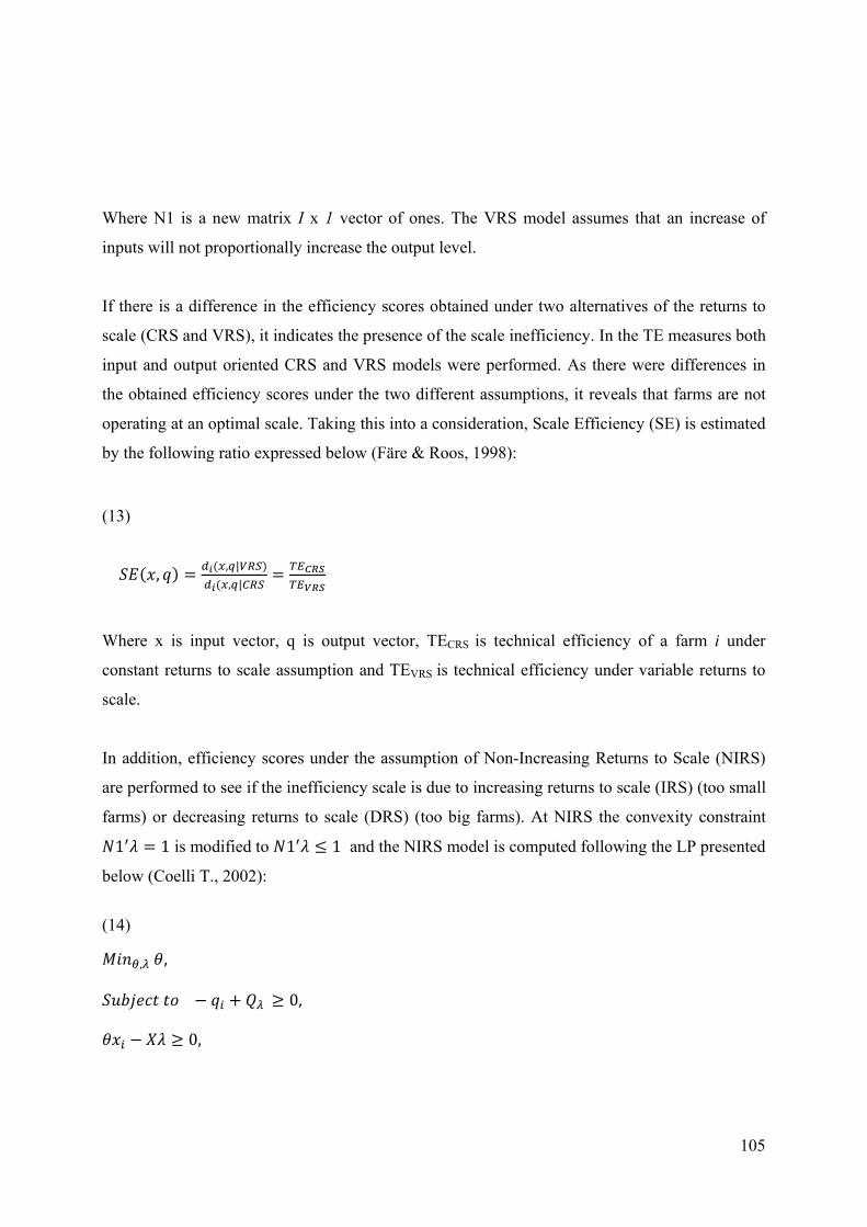
105

Where N1 is a new matrix I x 1 vector of ones. The VRS model assumes that an increase of

inputs will not proportionally increase the output level.

If there is a difference in the efficiency scores obtained under two alternatives of the returns to

scale (CRS and VRS), it indicates the presence of the scale inefficiency. In the TE measures both

input and output oriented CRS and VRS models were performed. As there were differences in

the obtained efficiency scores under the two different assumptions, it reveals that farms are not

operating at an optimal scale. Taking this into a consideration, Scale Efficiency (SE) is estimated

by the following ratio expressed below (Färe & Roos, 1998):

(13)

,, |

, |

Where x is input vector, q is output vector, TECRS is technical efficiency of a farm i under

constant returns to scale assumption and TEVRS is technical efficiency under variable returns to

scale.

In addition, efficiency scores under the assumption of Non-Increasing Returns to Scale (NIRS)

are performed to see if the inefficiency scale is due to increasing returns to scale (IRS) (too small

farms) or decreasing returns to scale (DRS) (too big farms). At NIRS the convexity constraint

1 1 is modified to 1 1 and the NIRS model is computed following the LP presented

below (Coelli T., 2002):

(14)

, ,

0,

0,

106

1 1, 0,

Output oriented approach: As previously mentioned both approaches are important in efficiency

measure, hence in addition to the input oriented model, output oriented TE measure is performed

for the three types of crops. Regardless of the orientation chosen, the TE scores are identical

under CRS assumption, therefore only an output-oriented model under the assumption of VRS

was calculated by solving the following LP problem (Coelli T. P., 2005):

(15)

, ,

0,

0,

1 1,

0,

where 1≤ <∞, and 1 is the proportional increase in outputs that could be achieved by the i-

th farm, given fixed inputs quantities.

107

5.1.2 Cost,revenueandallocativeefficiencyestimation

Input oriented approach: As input and output prices were available and behavioral assumption

like cost minimization or revenue maximization were made, the farm performance was estimated

by incorporating this information into the efficiency measurement. For the case of VRS cost

minimization, the input oriented DEA is conducted following the LP solution (Coelli T. P.,

2005):

(16)

, ∗ ∗

0,

∗ 0,

1,

0,

where wi represents the vector of input price in the farm i, xi* is the cost-minimising vector of

input quantity in the farm i, given the input price wi and the output level yi. The constraint

1 1 ensures the calculation of the minimum total costs for the farm i under VRS scale. The

Cost Efficiency (CE) for each farm is then calculated using the following ratio:

(17)

wixi ∗wixi

where, the numerator wixi ∗ is the minimum total cost obtained for the farm i and the

denominator wixi is the actual total costs observed in farm i.

The calculation of the allocative efficiency in the input-mix is presented in the equation below:

108

(18)

CAE = CE/TEinput-oriented

where CAE is the cost allocative efficiency. The CE is the product of both TE and AE

represented as CE = TE*AE (Farrell, 1957).

Output oriented approach: For the case of VRS revenue maximization, the following LP

problem was solved:

(19)

, ∗ ∗,

∗ 0,

0,

1 1, 0,

where pi is a vector of output prices in the farm i, ∗ is the revenue maximizing vector of output

quantities for farm i given the output prices pi and the input levels xi.

The overall revenue efficiency (RE) is calculated as the ratio of observed revenue to the

maximum revenue for the farm i (Coelli T. P., 2005).

(20)

piqi ∗

109

Revenue allocative efficiency in output-mix can be calculated as ratio of the RE and output

oriented TE of the farm i.

(21)

RAE = RE/TEoutput-oriented

Note: Performance Improvement Management DEA (PIM-DEA) software was used to obtain

scores of TE, SE, CE, CAE, RE and RAE efficiency scores.

5.2 Efficiencyanalysis

5.2.1 Technicalefficiencyoftomatofarms

The data set used in the technical efficiency estimation is a combination of common inputs used

in the tomato production process. Technical efficiency scores were obtained using tomato

saplings, fertilizer (artificial, crystal and manure), packing, machinery and labor as inputs and

tomato yields as output. In practice, very often farmers are not able to report all required input or

output variables. Descriptive statistics of variables used in the technical efficiency estimation for

tomato farms are presented in the table 33.

110

Table 33: Descriptive statistics of the input and output variables for TE estimation of tomato farms

Variable Unit Mean SD Minimum Maximum

Inputs

Saplings Saplings/ha 30,755.07 6,602.09 20,000.00 42,553.19

Artificial fertilizer Kg/ha 1,137.71 782.64 199.00 4,000.00

Manure Kg/ha 65,112.54 45,174.87 3,999.00 204,255.32

Crystalline fertilizer Kg/ha 761.97 1,024.30 61.50 6,153.85

Packing Boxes/ha 25,280.26 9,627.56 1,050.00 42,857.14

Machinery Fuel/ha 1,419.99 809.98 239.17 3,570.00

Labor Working

days/ha

569.68 229.40 280.00 1,244.00

Output

Tomato yield Kg/ha 144,462.41 37,320.62 77,777.78 245,000.00

Note: SD-standard deviation.

The share of tomato farms operating under input-oriented variable returns to scale and fully TE

is 67%, which is considerably higher than constant returns to scale model 47%.

Table 34: Average input oriented technical efficiency scores for tomato farms

Efficiency Mean SD Minimum Maximum

TECRS 0.889 0.135 0.583 1

TEVRS 0.957 0.075 0.731 1

The average TEInput-Oriented score for tomato farms under the assumption of VRS was estimated to

be 0.957, which indicates that on average tomato producers could further reduce the level of

inputs used and still remain at the same level of output produced. The quantity of inputs used by

technically inefficient farms was significantly higher compared to those TEInput-Oriented. This

111

applies particular to artificial fertilizer (46%), manure (13%) and fuel for machinery (12%). As

the TEInput-oriented scores are calculated under two different scenarios CRS and VRS, scale

efficiency (SE) is estimated to examine if the tomato farms are operating at optimal scale. The

SEInput-Oriented score ranges from 0.592 up to 1, with an average score of 0.926 showing that

tomato farms are operating close to optimal scale. No more than 18 out of 38 tomato farms were

operating at fully optimal scale. In addition, efficiency scores under the assumption of non-

increasing returns to scale (NIRS) are performed to see if the inefficiency scale is due to

increasing returns to scale (IRS) (too small farms) or decreasing returns to scale (DRS) (too big

farms). The estimated results under the NIRS scenario show that a majority (18 out of 20) of the

tomato farms are operating inefficiently at scale due to being too small.

Given that efficiency scores are too sensitive to measurements and sampling errors, the real

efficiency scores may be lower than those obtained. Boostrapping procedure permits valid

inference and improves statistical efficiency in the second-stage regression (Simar L., and

Wilson W. P., 2007). Simar and Wilson (2007) argue that two-stage approach may be invalid as

it does not describe the data-generating process in the model and it suffers from serial correlation

of the estimated efficiencies. Simar and Wilson (2007) show that 'truncated regression combined

with bootstrapping as a resampling technique best overcomes the unknown serial correlation

(Wanke P., 2016). Therefore, bootstrapping for TEInput-Oriented measures was performed, to

encounter such problems by estimating confidence intervals and bias-corrected TEInput-Oriented

scores.

Table 35: Bias-corrected efficiency scores for tomato farms under VRS assumption

Orientation Bias-corrected efficiency score

Bias-corrected 95% CI†

SD of bias-corrected efficiency score

Input 0.954 0.942-0.958 0.078 Note: CI-confidence interval; † 2000 replications were used for bootstrapping (Simar L., and Wilson W. P., 2007) .

Bias-corrected efficiency scores presented in the table above shows that there is a little more

space for performance improvement of the tomato farms. Slacks of the bias-corrected scores

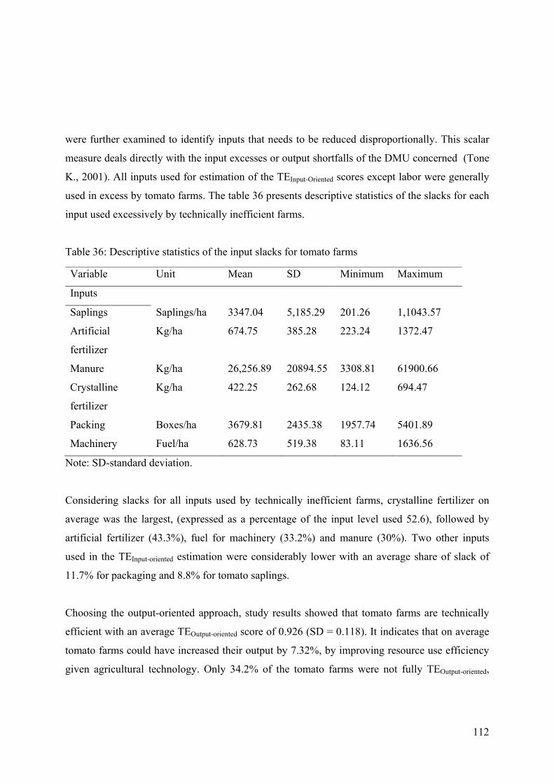
112

were further examined to identify inputs that needs to be reduced disproportionally. This scalar

measure deals directly with the input excesses or output shortfalls of the DMU concerned (Tone

K., 2001). All inputs used for estimation of the TEInput-Oriented scores except labor were generally

used in excess by tomato farms. The table 36 presents descriptive statistics of the slacks for each

input used excessively by technically inefficient farms.

Table 36: Descriptive statistics of the input slacks for tomato farms


Inputs

Saplings Saplings/ha 3347.04 5,185.29 201.26 1,1043.57

Artificial

fertilizer

Kg/ha 674.75 385.28 223.24 1372.47

Manure Kg/ha 26,256.89 20894.55 3308.81 61900.66

Crystalline

fertilizer

Kg/ha 422.25

262.68 124.12 694.47

Packing Boxes/ha 3679.81 2435.38 1957.74 5401.89

Machinery Fuel/ha 628.73 519.38 83.11 1636.56


Considering slacks for all inputs used by technically inefficient farms, crystalline fertilizer on

average was the largest, (expressed as a percentage of the input level used 52.6), followed by

artificial fertilizer (43.3%), fuel for machinery (33.2%) and manure (30%). Two other inputs

used in the TEInput-oriented estimation were considerably lower with an average share of slack of

11.7% for packaging and 8.8% for tomato saplings.

Choosing the output-oriented approach, study results showed that tomato farms are technically

efficient with an average TEOutput-oriented score of 0.926 (SD = 0.118). It indicates that on average

tomato farms could have increased their output by 7.32%, by improving resource use efficiency

given agricultural technology. Only 34.2% of the tomato farms were not fully TEOutput-oriented,

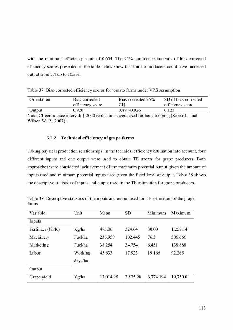
113

with the minimum efficiency score of 0.654. The 95% confidence intervals of bias-corrected

efficiency scores presented in the table below show that tomato producers could have increased

output from 7.4 up to 10.3%.

Table 37: Bias-corrected efficiency scores for tomato farms under VRS assumption




Output 0.920 0.897-0.926 0.125 Note: CI-confidence interval; † 2000 replications were used for bootstrapping (Simar L., and Wilson W. P., 2007) .

5.2.2 Technicalefficiencyofgrapefarms

Taking physical production relationships, in the technical efficiency estimation into account, four

different inputs and one output were used to obtain TE scores for grape producers. Both

approaches were considered: achievement of the maximum potential output given the amount of

inputs used and minimum potential inputs used given the fixed level of output. Table 38 shows

the descriptive statistics of inputs and output used in the TE estimation for grape producers.

Table 38: Descriptive statistics of the inputs and output used for TE estimation of the grape farms


Inputs

Fertilizer (NPK) Kg/ha 475.06 324.64 80.00 1,257.14


Marketing Fuel/ha 38.254 34.754 6.451 138.888

Labor Working

days/ha

45.633 17.923 19.166 92.265

Output

Grape yield Kg/ha 13,014.95 3,525.98 6,774.194 19,750.0

114

The share of grape farms being fully efficient was 35.3% under CRS assumption and 58.8%

under VRS. The average TEInput-Oriented score under CRS assumption was 0.834 (SD=0.181) and

0.905 (SD=0.148) for VRS assumption. It can be seen that grape farmers use more inputs than

were needed to obtain the same amount of output. On average grape producers could have

reduced the quantity of inputs used by a maximum of 16.6% and still gain the same level of

output. The average SE score was estimated to be 0.920, indicating that most of the grape

producers were operating at relatively high optimal scale. The scale inefficiency was present at

64.7% or 22 out of 34 grape farms. The estimated results under NIRS model showed that scale

inefficiency was mainly coming from small holder farms.

Table 39: Bias-corrected efficiency scores for grape farms under VRS assumption




Input 0.897 0.871-0.906 0.156 Note: CI-confidence interval; † 2000 replications were used for bootstrapping.

DEA bootstrapping method indicates that the efficiency estimates for grape farms are likely to

vary from 0.871 to 0.906, which also illustrates the sensitivity of efficiency estimates to

variations in sample composition. The LP solution presented above may not always identify all

efficiency. Therefore, after the efficiency scores were obtained, slacks were calculated and

examined for the farms being in the best practice frontier. The main intention was to find out the

presence of grape farms being weakly efficient and see the possibilities of further reduction of

any individual input at different proportion. The calculated slacks showed that there was no

chance to further reduce any of the individual inputs as 58.8% of the farms being fully efficient

had zero slacks. Nine out of fourteen or 64% of the inefficient grape farms were using fertilizer

NPK in excessive amounts.

In the output-oriented approach, the average TEOutput-oriented score under VRS model was

estimated to be 0.906 (SD = 0.144) with a minimum TEOutput-oriented score of 0.512. This result

115

shows that grape producers on average could have increased the level of output by 9.4% and still

keep the same level of inputs used.

Table 40: Bias-corrected efficiency scores for grape farms under VRS assumption




Output 0.898 0.877-0.906 0.151 Note: CI-confidence interval; † 2000 replications were used for bootstrapping. No difference is observed between input-oriented and output-oriented approaches of the TE

scores, suggesting that farms do not vary in terms of production assortment and quality.

5.2.3 Technicalefficiencyofapplefarms

The estimated TE scores of the apple farms were obtained using four different inputs and one

output. Both input and output oriented models under CRS and VRS assumptions were

performed. Descriptive statistics of the inputs and output used in the estimation of TE at apple

farms is presented in the following table.

Table 41: Descriptive statistics of the inputs and output used for TE estimation of the apple farms


Inputs

Fertilizer (NPK) Kg/ha 744.59 406.14 200.00 1,250.00


Marketing Boxes/ha 1,399.70 1,042.13 4,250.00 220.00

Labor Working

days/ha

61.22 36.14 17.26 154.00

Output

Apple yield Kg/ha 54,339 38,795.60 10,000 170,000

116

The share of apple farms being technically efficient under CRS assumption was 23.52 %. The

share of technically efficient farms was shown to be higher under VRS assumption 41.17%. The

mean of TE Input-oriented score under CRS was 0.695 (SD = 0.242) and ranges from 0.254 and 1.00.

The average of TE Input-oriented under VRS was estimated to be 0.876 (SD = 0.163) with the range

of 0.428 and 1.00. This result indicates that apple producers on average could reduce the amount

of inputs used by 12.38% and keep the same level of the output produced. The mean of SE is

0.799 (SD = 0.22) with the range of 0.254 to 1.000. The percentage of farms operating at an

optimal scale was 25.8, for the majority of the farms 51.6% the scale inefficiency was due to

being too small. The percentage of the farms being scale inefficient due to being too big in size

was smaller (22.5%).

Table 42: Bias-corrected efficiency scores for apple farms under VRS assumption




Input 0.862 0.826-0.876 0.172 Note: CI-confidence interval; † 2000 replications were used for bootstrapping.

Slacks were calculated and examined further for the farms being in the best practice frontier. The

number of total farms being technically efficient in VRS input oriented model was 11 and out of

them 2 were found to be weakly technically efficient having slacks in the same inputs (labor and

machinery). The table below presents descriptive statistics of the slacks found at each input used

excessively by the technically inefficient farms.

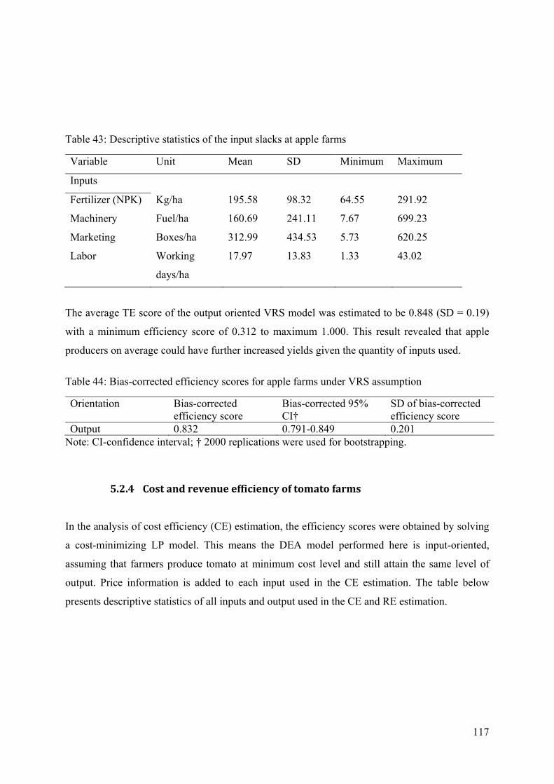
117

Table 43: Descriptive statistics of the input slacks at apple farms


Inputs

Fertilizer (NPK) Kg/ha 195.58 98.32 64.55 291.92


Marketing Boxes/ha 312.99 434.53 5.73 620.25

Labor Working

days/ha

17.97 13.83 1.33 43.02

The average TE score of the output oriented VRS model was estimated to be 0.848 (SD = 0.19)

with a minimum efficiency score of 0.312 to maximum 1.000. This result revealed that apple

producers on average could have further increased yields given the quantity of inputs used.

Table 44: Bias-corrected efficiency scores for apple farms under VRS assumption




Output 0.832 0.791-0.849 0.201 Note: CI-confidence interval; † 2000 replications were used for bootstrapping.

5.2.4 Costandrevenueefficiencyoftomatofarms In the analysis of cost efficiency (CE) estimation, the efficiency scores were obtained by solving

a cost-minimizing LP model. This means the DEA model performed here is input-oriented,

assuming that farmers produce tomato at minimum cost level and still attain the same level of

output. Price information is added to each input used in the CE estimation. The table below

presents descriptive statistics of all inputs and output used in the CE and RE estimation.

118

Table 45: Descriptive statistics of the input and output variables for CE and RE estimation of tomato farms


Inputs

Saplings EUR/ha 3,947.63 1,058.97 2,418.98 7,500.00

Fertilizers EUR/ha 2,464.82 1,666.06 362.5 10,769.23

Irrigation EUR/ha 384.32 353.31 53.00 1,800.00

Marketing EUR/ha 9,311.95 2,946.02 2,167.90 16,000.00

Machinery EUR/ha 1,305.37 730.13 421.00 5,030.74

Labor EUR/ha 6,921.69 3,096.53 3,700.00 17,074.47

Output

Tomato sales EUR/ha 36,771.25 9,299.75 19,444.44 61,250.00


Table 46: Descriptive statistics of the cost efficiency scores of tomato farms


CECRS 0.681 0.122 0.493 1

CEVRS 0.781 0.119 0.589 1

Note: CE-cost efficiency; VRS-variable returns to scale; CRS-constant returns

to scale; SD-standard deviation.

The mean CE score under VRS assumption is 0.781, which implies that given the input prices,

tomato farmers could minimize total costs by 31.9%, without worsening the current level of

output. The share of CE farms under VRS is relatively small, only 10% or 4 out of 38 tomato

farms were fully costly efficient. Comparing input by input, CE farms were having in general

lower input costs than the mean input cost of the total sample.

119

Table 47: Descriptive statistics of allocative (input-mix) efficiency scores of tomato farms


CAECRS 0.771 0.108 0.570 1

CAEVRS 0.816 0.108 0.589 1

Note: CAE- cost allocative efficiency; VRS-variable returns to scale; CRS-constant returns


The mean of cost allocative (input-mix) efficiency (CAE) score under VRS assumption across

farms is 0.816, indicating that there is sufficient space (18.3%) for performance improvement

through the use of inputs in optimal proportions, given their prices and the production

technology. The correlation coefficient of CEVRS scores with AEVRS is stronger (0.847, p=0.000),

compared to TEInput-OrientedVRS scores (0.455, p=0.004), demonstrating that improvements in

AEInput-Mix would have higher impact on CE improvements. The table below presents the

distribution of the input-oriented technical, cost and cost allocative efficiency scores for 38

tomato farms.

Table 48: Distribution of the input-oriented efficiency scores of tomato farms

Efficiency range

TEVRS no. of farms %

CEVRS no. of farms %

CAEVRS no. of farms %

=1 25 65.7 4 10.5 4 10.5 >0.9 < 1.0 5 13.1 2 5.2 4 10.5 >0.8 < 0.9 6 15.7 10 26.3 13 34.2 >0.7 < 0.8 2 5.2 8 21.0 10 26.3 >0.6 < 0.7 0 0 12 31.5 6 15.7 >0.5 < 0.6 0 0 2 5.2 1 2.6 <0.5 0 0 0 0 0 0 38 100 38 100 38 100

The efficiency scores were further investigated in regard to the size-efficiency relationships. The

obtained correlation coefficients did not show significant relationships between farm size and

TEInput-oriented, CE and CAE efficiency scores.

120

2000015000100005000 40003000200010000

1 .0

0 .9

0 .8

0 .7

0 .6

18000150001200090006000

1 .0

0 .9

0 .8

0 .7

0 .6

15000100005000

T otal input s EUR/ha

Allo

cati

ve e

ffic

ienc

y sc

ores

T ot al mach ine ry cost s EUR/ha

Labor EUR/ha T ot al marke t ing cost s EUR/ha

Figure 39: Scatter-plot of the CAE scores and inputs used by tomato farms

The revenue efficiency was estimated from the perspective of output based models. The method

sought to identify inefficiency of the tomato farms as proportional increase in output production,

by holding inputs fixed.

Table 49: Descriptive statistics of the revenue efficiency scores of tomato farms


RECRS 0.863 0.137 0.598 1

REVRS 0.926 0.124 0.603 1

Note: RE-revenue efficiency; VRS-variable returns to scale; CRS-constant returns


The mean of RE score under VRS assumption is 0.926, indicating that on average tomato

producers could maximize their revenues by 7.4%, given the input costs. On average, tomato

farms have a tendency to be more technical efficient followed by scale, revenue, cost allocative

having the lowest average on cost efficiency.

121

Table 50: Distribution of the output-oriented efficiency scores of tomato farms

Efficiency range


REVRS no. of farms %

=1 25 65.78 26 68.42 >0.9 < 1.0 3 7.89 2 5.26 >0.8 < 0.9 1 2.63 2 5.26 >0.7 < 0.8 6 15.78 4 10.52 >0.6 < 0.7 3 7.89 4 10.52 >0.5 < 0.6 0 0 0 0 <0.5 0 0 0 0

Total 38 100 38 100

It can be seen from the distribution of TEVRS input and output oriented efficiency scores that

there is no significant difference among the efficiency ranges. In both approaches, 25 farms

appeared to be fully technically efficient, with slight changes in other efficiency classes. The

distribution of farms completely changes when cost-minimization and revenue-maximization

objective functions were imposed. In this regard, tomato farmers were performing perfectly in

marketing their product. The situation is notably different when CEVRS was estimated, where

only 4 or 10.5% of the farms belonged to the fully cost efficient class. Taking into a

consideration that many of the farms were full TE and RE but few of them CE, it demonstrates

that input prices were playing an important role on farm performance when cost-minimization

objective function was considered.

5.2.5 Costandrevenueefficiencyofgrapefarms Similar to the section above, cost minimization and revenue maximization LP-s for grape

producers were solved, by adding up prices to the inputs used and output produced. Variables

included in the CE and RE analysis are presented in table 51.

122

Table 51: Descriptive statistics of the input and output variables for CE and RE estimation of grape farms


Inputs

Fertilizer (NPK) EUR/ha 203.05 155.82 32.73 666.67

Machinery EUR/ha 290.87 128.13 91.80 704.00

Marketing EUR/ha 93.93 68.942 22.00 300.00

Labor EUR/ha 683.34 266.84 267.50 1,365.00

Output

Grape sales EUR/ha 4,113.31 1,435.87 1,913.33 7,258.00


Table 52: Descriptive statistics of the cost efficiency scores of grape farms


CECRS 0.424 0.156 0.237 1

CEVRS 0.689 0.189 0.334 1

Note: CE-cost efficiency; VRS-variable returns to scale; CRS-constant returns


The obtained CEVRS scores, show that on average, grape farmers could reduce total costs by 31%

without any reductions in the output level. The share of grape farms operating on the production

frontier and having zero slacks was 8.8%.

Table 53: Descriptive statistics of allocative (input-mix) efficiency scores of grape farms


CAECRS 0.519 0.184 0.270 1

CAEVRS 0.766 0.178 0.334 1

Note: CAE- cost allocative efficiency; VRS-variable returns to scale; CRS-constant returns


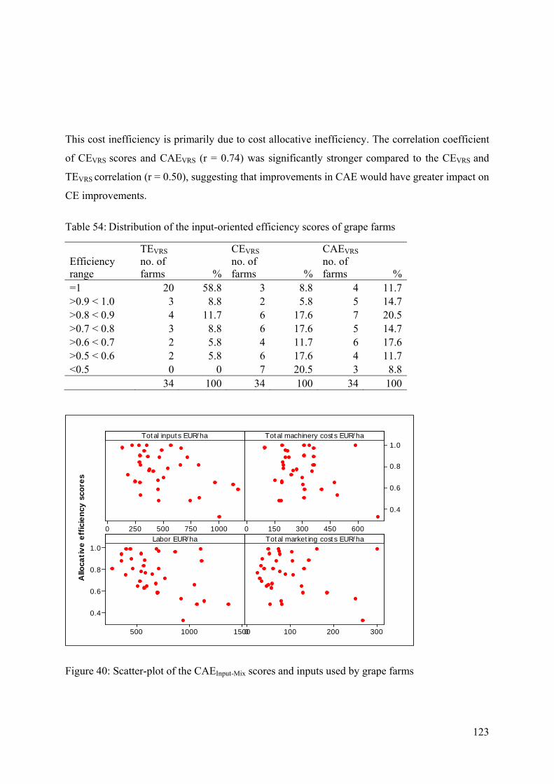
123

This cost inefficiency is primarily due to cost allocative inefficiency. The correlation coefficient

of CEVRS scores and CAEVRS (r = 0.74) was significantly stronger compared to the CEVRS and

TEVRS correlation (r = 0.50), suggesting that improvements in CAE would have greater impact on

CE improvements.

Table 54: Distribution of the input-oriented efficiency scores of grape farms

Efficiency range




=1 20 58.8 3 8.8 4 11.7 >0.9 < 1.0 3 8.8 2 5.8 5 14.7 >0.8 < 0.9 4 11.7 6 17.6 7 20.5 >0.7 < 0.8 3 8.8 6 17.6 5 14.7 >0.6 < 0.7 2 5.8 4 11.7 6 17.6 >0.5 < 0.6 2 5.8 6 17.6 4 11.7 <0.5 0 0 7 20.5 3 8.8 34 100 34 100 34 100

10007505002500 6004503001500

1.0

0.8

0.6

0.4

15001000500

1.0

0.8

0.6

0.4

3002001000

Total inputs EUR/ha

Allo

cati

ve e

ffic

ienc

y sc

ores

Total machinery costs EUR/ha

Labor EUR/ha Total marketing costs EUR/ha

Figure 40: Scatter-plot of the CAEInput-Mix scores and inputs used by grape farms

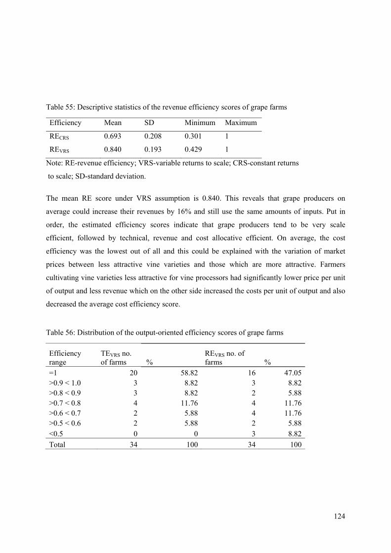
124

Table 55: Descriptive statistics of the revenue efficiency scores of grape farms


RECRS 0.693 0.208 0.301 1

REVRS 0.840 0.193 0.429 1

Note: RE-revenue efficiency; VRS-variable returns to scale; CRS-constant returns


The mean RE score under VRS assumption is 0.840. This reveals that grape producers on

average could increase their revenues by 16% and still use the same amounts of inputs. Put in

order, the estimated efficiency scores indicate that grape producers tend to be very scale

efficient, followed by technical, revenue and cost allocative efficient. On average, the cost

efficiency was the lowest out of all and this could be explained with the variation of market

prices between less attractive vine varieties and those which are more attractive. Farmers

cultivating vine varieties less attractive for vine processors had significantly lower price per unit

of output and less revenue which on the other side increased the costs per unit of output and also

decreased the average cost efficiency score.

Table 56: Distribution of the output-oriented efficiency scores of grape farms

Efficiency range


REVRS no. of farms %

=1 20 58.82 16 47.05 >0.9 < 1.0 3 8.82 3 8.82 >0.8 < 0.9 3 8.82 2 5.88 >0.7 < 0.8 4 11.76 4 11.76 >0.6 < 0.7 2 5.88 4 11.76 >0.5 < 0.6 2 5.88 2 5.88 <0.5 0 0 3 8.82

Total 34 100 34 100

125

An almost similar distribution is shown between TE input and output scores among different

efficiency classes. In total 20 out of 34 farms were fully technical efficient in input and output

oriented approach. The distribution of the efficiency scores changes slightly for the revenue

maximization approach. A smaller number of farms belongs to the range fully efficient and

movement of the farms towards lower RE efficiency scores is mainly due to price variations

among the grape varieties farmers cultivate. The cost-minimization approach presents a different

situation, where only 3 out of 34 farms belongs to the full cost efficient class. As for tomato

producers, input costs are a determinant factor for the farm performance level.

5.2.6 Costandrevenueefficiencyofapplefarms In the cost efficiency measure, the objective function was to minimize the costs of the inputs

used given the same level of output. Price information was added to each input used in the TE

measure. The table 57 presents descriptive statistics of the costs of all inputs and output used in

the CE and RE estimation.

Table 57: Descriptive statistics of the input and output variables costs of apple farms


Inputs

Fertilizer (NPK) EUR/ha 349.04 239.49 60 976.56

Machinery EUR/ha 245.28 278.23 27.77 1,150

Marketing EUR/ha 663.87 517.96 110 2,125

Labor EUR/ha 895.84 505.28 258.9 1,970

Output

Apple sales EUR/ha 1,8061.56 1,1853.57 3,300 53,833.33


The overall mean of the CE score in VRS model was estimated to be 0.613 (SD = 0.241) with

the minimum range of 0.211. On average, apple producers could have decreased the input costs

126

by 38.7% and still achieve the same level of output. The share of apple farms being fully cost

efficient with zero slacks was 9.6%. The average CAE score in the VRS model was 0.697 (SD =

0.230) and the minimum score was 0.214, showing that apple producers on average could have

improved their performance with a better mix of inputs and the prices.

Table 58: Distribution of the input-oriented efficiency scores of apple farms

Efficiency range




=1 14 45.16 3 9.67 3 9.67 >0.9 < 1.0 3 9.67 0 0.00 2 6.45 >0.8 < 0.9 5 16.12 5 16.12 10 32.25 >0.7 < 0.8 5 16.12 4 12.90 4 12.90 >0.6 < 0.7 2 6.45 6 19.35 1 3.22 >0.5 < 0.6 0 0.00 4 12.90 4 12.90 <0.5 2 6.45 9 29.03 7 22.58 31 100 31 100 31 100

10007505002500 10007505002500

100

80

60

40

20

200015001000500

100

80

60

40

202000150010005000

Fertilizer EUR/ha

Allo

cati

ve e

ffic

ienc

y sc

ores

Total machinery costs EUR/ha

Labor EUR/ha Total marketing costs EUR/ha

Figure 41: Scatter-plot of the CAE scores and inputs used by apple farms

127

The average of the RE score in the VRS model was 0.848 (SD = 0.190) with a minimum of

0.321. Based on the obtained results we could say that apple producers can improve their farm

performance through further increase of revenues given the input costs. The share of farms being

fully revenue efficient was 45.16%. Looking at all estimated efficiency scores, it is shown that

apple producers on average are performing relatively well in terms of technical efficiency which

was the highest on average, followed by revenue efficiency and scale efficiency. The average

cost efficiency score was the lowest, indicating high variation of market input output prices

among the farmers.

5.3 Regressionanalysis

5.3.1 Regressionanalysisoftomatofarms

Regression analysis was performed to find out how the variation of the efficiency scores could

be explained by other farm characteristics. The truncated regression model is presented in the

following function:

(22)

assume that is the deterministic part of the classical regression model. Then

, i=1,....,n

where

| ~ 0, ,

so that

| ~ , .

The interest here is on the distribution of given that is greater than the truncation point a.

The conditional mean is therefore a nonlinear function of a, σ, x, β. In the given model

128

represents the efficiency score of the farm i; are unknown parameters to be estimated; =1

to n are explanatory variables for the farm; and is an error term which is independently and

normally distributed with mean 0 and constant variance (Greene H.W., 2003). Truncated

regression analysis were performed using EViews (version 9) software.

The variables used to explain the variation of the efficiency scores were: 1. farmer's age (in

years); 2. education (in years); 3. household size (number of the family members living regularly

at farm house); 4. employment (number of the family members working regularly at farm); 5.

number of income sources; 6.experience in agriculture (number of years active in farming); 7.

farm size (in ha); 8. number of parcels; and 9. number of cultivated crops. After testing,

redundant explanatory variables were omitted from the initial model. Regression coefficients of

the best fitted model for tomato farms are presented in the table 59.

129

Table 59: Regression results of the efficiency scores and other tomato farm characteristics

Independent variables Coefficient

TEVRS

Coefficient

CEVRS

Coefficient

CAEVRS

SE

Household size 0.004266 *

(0.002107)

0.007252 *

(0.003132)

- -

Number of income sources 0.000536

(0.000752)

-0.001093

(0.001100)

-0.001389

(0.001038)

0.025762

(0.021644)

Number of parcels -0.005013

(0.003727)

- - -

Farmer's age - 0.002800

(0.002373)

0.002751

(0.002247)

-0.002807

(0.002210)

Number of cultivated crops - -0.016443 *

(0.007377)

-0.016044

(0.009240)

-

Employment - - - -0.012816

(0.007057)

Farm size - - 0.014255

(0.012501)

0.028582 *

(0.011803)

Experience - - - -0.001691

(0.001472)

Constant 0.931762

(0.030978)

0.692866

(0.120397)

0.768795

(0.111843)

1.033831

(0.101204)

Σ 0.078780 0.116465 0.110163 0.102695

Log-likelihood 44.20566 30.32861 32.38696 34.74596

Note: TE, technical efficiency; CE, cost efficiency; CAE, allocative efficiency; SE, Scale efficiency; VRS, variable returns to scale. Asterisks *, represent statistical significance at the 5% level. Number in parenthesis and italics are standard errors.

The obtained coefficient with truncated regression analysis shows that household size was

positively correlated and significantly determined TEVRS and CEVRS scores of the tomato farms.

The TEVRS scores were negatively correlated with the number of parcels in the farm, indicating

130

that the smaller the number of parcels, the higher TEVRS scores were for the farm. A significant

negative effect on technical efficiency captured by Simpson’s index and the number of plots was

also found in the study by Sauer J., et al., 2014 and Di Falco et al., 2010. The number of income

sources of the farm was positively correlated with the TEVRS scores, even though this has not

been proven to be statistically significant. Besides household size, number of cultivated crops on

the farm had significant but negative impact on the CEVRS scores. This indicates that diversified

farms tend to have greater economic inefficiency than those specialized in smaller number of

cultivated crops. The other remaining factors of the CEVRS model had no significant effects on

the CE scores variation. Farm size in terms of cultivated ha is the only explanatory variable that

has a significant positive effect on the SE scores. Showing that farm size significantly determines

the scale operation of the farm. This was also demonstrated by the estimated efficiency scores

under NIRS scenario.

5.3.2 Regressionanalysisofgrapefarms

Using the method described in the section above, technical, cost-allocative and scale efficiency

scores of the grape farms were related to factors that describe other farm characteristics. Finding

out factors that could explain the differences in efficiency scores among farms is of major

interest to farmers and other stakeholders as by improving these factors opportunities to improve

farm performance will be better. In the truncated regression model (equation 22) technical, cost-

allocative and scale efficiency scores were related to: 1. farmer's age (in years); 2. farmer's

education (in years); 3. household size (number of the family members living regularly at farm

house); 4. employment (number of the family members working regularly at farm); 5.experience

in agriculture (number of years active in farming); 6. farm size (in ha); 7. number of parcels; and

8. number of cultivated crops. A coefficient diagnostics test was performed and redundant

variables were omitted from the initial model. Regression coefficients of the best fitted model are

presented in the table 60.

131

Table 60: Regression results of the TE, CAE and SE scores and other grape farm characteristics


TEVRS

Coefficient

CAEVRS

SE

Household size 0.011860*

(0.005279)

- -

Farmer's age - 0.004970

(0.004299)

-0.003567

(0.002718)

Education 0.018711*

(0.007377)

-0.023694*

(0.011241)

0.020392**

(0.007205)

Number of parcels - - -

Number of cultivated crops -0.018068

(0.012677)

-0.018099

(0.016113)

0.024886*

(0.010045)

Employment -0.024317

(0.015315)

0.016954

(0.017785)

-

Farm size 0.013459

(0.007503)

- -

Experience - -0.002471

(0.004193)

0.004941

(0.002659)

Constant 0.643859

(0.113482)

0.886039

(0.207073)

0.606183

(0.127409)

Σ 0.127892 0.176793 0.111353

Log-likelihood 25.59841 14.58928 29.68857

Note: TE, technical efficiency; CAE, allocative efficiency; SE, Scale efficiency; VRS, variable

returns to scale. Asterisks *, represent statistical significance at the 5% and ** 1% level. Number in

parenthesis and italics are standard errors. None of the independent variables included in the censored

regression model were statistically significant in explaining the variation of the CE scores.

The level at which grape farmers were educated was positively correlated and significantly

determined the variation of technical and scale efficiency scores. Farmer's education has

significant impact on cost-allocative efficiency scores but it was shown to be negatively

132

correlated. This could be explained by the education profile of the grape producers. Most of

those who are considered to be better educated (high school or university) graduated in

agronomy, meaning that they know much more about cultivation of grapes and production

techniques but a majority does not keep records of their expenses and revenues. As a result, they

are not able to conduct more specialized duties like calculation of the production costs or their

profit margins, which is essential for farm performance improvement and making better

investments decisions. Household size was positively correlated and appears to have significant

impact on technical efficiency suggesting that bigger families are more efficient in the use of

resources. The number of cultivated crops in a farm was shown to have a positive and significant

effect on farm scale efficiency, indicating that farmers who diversify their crop portfolio more do

perform on a more optimal scale.

133

5.3.3 Regressionanalysisofapplefarms The technical, cost, and cost-allocative efficiency scores were regressed to the same variables as

in the previous regression models with tomato and grape producers. Initial regression model was

simplified through backward elimination of the redundant variables and the best fitted models

and estimated coefficients for three types of the estimated efficiency (TE, CE and CAE) are

presented in the following table.

Finding out factors that could explain the differences in efficiency scores among farms are of

major interest to farmers and other stakeholders as by improving these factors, opportunities to

improve farm performance will be better. In the censored regression model (see equation 13)

technical, cost-allocative and scale efficiency scores were related to: 1. farmer's age (in years); 2.

farmer's education (in years); 3. household size (number of the family members living regularly

at farm house); 4. employment (number of the family members working regularly at farm); 5.

experience in agriculture (number of years active in farming); 6. farm size (in ha); 7. number of

parcels; and 8. number of cultivated crops. Coefficient diagnostics test was performed and

redundant variables were omitted from the initial model. Regression coefficients of the best fitted

model are presented in the table 61.

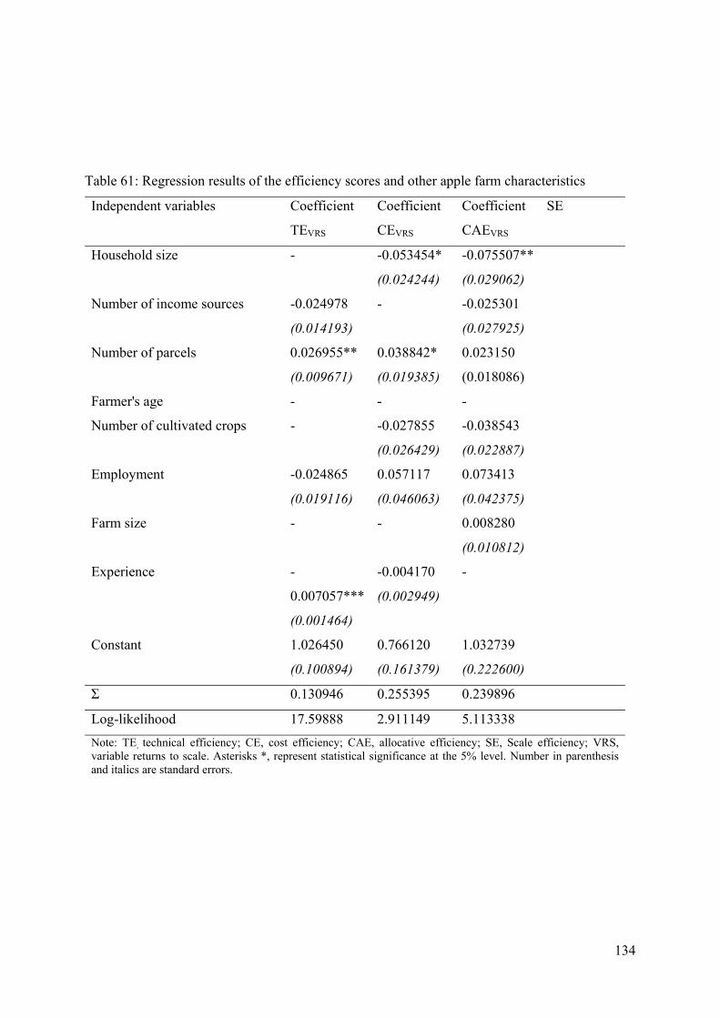
134

Table 61: Regression results of the efficiency scores and other apple farm characteristics


TEVRS

Coefficient

CEVRS

Coefficient

CAEVRS

SE

Household size - -0.053454*

(0.024244)

-0.075507**

(0.029062)

Number of income sources -0.024978

(0.014193)

- -0.025301

(0.027925)

Number of parcels 0.026955**

(0.009671)

0.038842*

(0.019385)

0.023150

(0.018086)

Farmer's age - - -

Number of cultivated crops - -0.027855

(0.026429)

-0.038543

(0.022887)

Employment -0.024865

(0.019116)

0.057117

(0.046063)

0.073413

(0.042375)

Farm size - - 0.008280

(0.010812)

Experience -

0.007057***

(0.001464)

-0.004170

(0.002949)

-

Constant 1.026450

(0.100894)

0.766120

(0.161379)

1.032739

(0.222600)

Σ 0.130946 0.255395 0.239896

Log-likelihood 17.59888 2.911149 5.113338

Note: TE, technical efficiency; CE, cost efficiency; CAE, allocative efficiency; SE, Scale efficiency; VRS, variable returns to scale. Asterisks *, represent statistical significance at the 5% level. Number in parenthesis and italics are standard errors.

135

6.ENVIRONMENTALEFFICIENYANALYSIS This chapter presents the results of the extended efficiency measure and analysis for tomato,

grape and apple producers. The extension considered involves environmental variables (soil

quality and number of cultivated varieties given the cultivated crop) that could influence the

efficiency of a farm.

6.1 Environmentalefficiencyestimation In addition to the traditional inputs and output data, we introduced environmental data into the

environmental efficiency analysis that could affect the efficiency level of a farm. The model of

TE estimation was extended by adjusting two other variables that describe the environment, such

as soil quality and the number of cultivated varieties within a given crop (tomato, grape or

apple).

The soil quality index (SQI) was used as an indicator of the quality of land where a particular

crop was cultivated. The two stage method was performed to determine the direction of influence

of the SQI into TE scores. In the first stage, an output oriented TE model under VRS assumption

(as in equation 24) was performed, and after, in the second stage the obtained TE scores from the

first stage method has been regressed upon the SQI, using the truncated regression method as in

equation 23. The positive sign of the coefficient of the SQI indicated the direction of influence

into TE scores. Moreover, on average the estimated SQI of cultivated land was higher than the

SQI of uncultivated land (SQI 6% higher in cultivated land). Taking these results into an

account, we considered the SQI of cultivated land as a positive or desirable output which is

jointly produced in addition to the traditional output (tomato, grape and apple). The Shannon's

diversity index (SHDI) was considered as measure of biodiversity, calculated based on the

number of cultivated varieties within given crop. In several studies SHDI is considered as

positive output in addition to the traditional outputs in agriculture e.g. (Sipiläinen T., 2008) and

(Solovyeva I. and Nuppenau A. E., 2013). At the farm level, cultivation of the different varieties

of a specific crop on given area is related to conservation of biological variation, which is a good

136

that the society values. Following the Coelli (2005) model, both environmental variables SQI

and SHDI were introduced in the LP as positive outputs. The output-oriented TEVRS LP changes

as following in the LP (Coelli T. P., 2005):

(23)

, ,

0,

0,

0,

1 1,

0,

where "positive effect" environmental variables were denoted by the Lx1 vector for the i-th

farm and by the LxN matrix Z for the full sample. The sign on the dual variable associated with

the Z-variable has indicated whether the variable has a desirable on non-desirable effect upon the

efficiency of a farm. The i-th farm is compared with a theoretical frontier farm that has an

environment that is no better than the one of the i-th farm.

6.1.1 Environmentalefficiencyresultsoftomatofarms

In the environmental efficiency analysis, the method seeking to identify inefficiency of the

tomato farms as equi-proportional increase in outputs produced by holding the quantities of the

inputs used fixed. The environmental variables were directly introduced into the LP formulation

as ordinary variables. The purpose of this analysis was to evaluate the effect of the inclusion of

environmental variables into the farm performance assessment. Descriptive statistics of the

variables included in the environmental efficiency measure are shown in the table below.

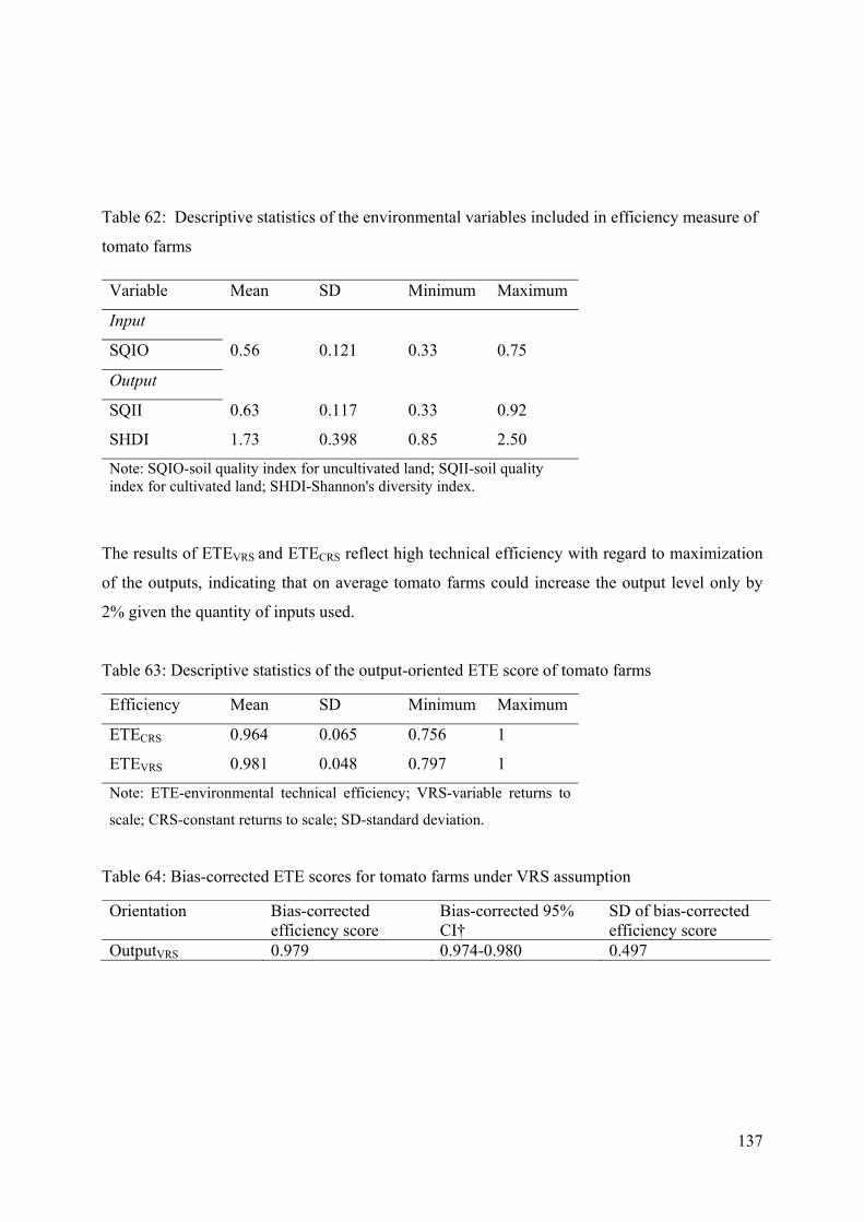
137

Table 62: Descriptive statistics of the environmental variables included in efficiency measure of

tomato farms

Variable Mean SD Minimum Maximum

Input

SQIO 0.56 0.121 0.33 0.75

Output

SQII 0.63 0.117 0.33 0.92

SHDI 1.73 0.398 0.85 2.50

Note: SQIO-soil quality index for uncultivated land; SQII-soil quality index for cultivated land; SHDI-Shannon's diversity index.

The results of ETEVRS and ETECRS reflect high technical efficiency with regard to maximization

of the outputs, indicating that on average tomato farms could increase the output level only by

2% given the quantity of inputs used.

Table 63: Descriptive statistics of the output-oriented ETE score of tomato farms


ETECRS 0.964 0.065 0.756 1

ETEVRS 0.981 0.048 0.797 1

Note: ETE-environmental technical efficiency; VRS-variable returns to

scale; CRS-constant returns to scale; SD-standard deviation.

Table 64: Bias-corrected ETE scores for tomato farms under VRS assumption




OutputVRS 0.979 0.974-0.980 0.497

138

Table 65: Distribution of the output-oriented efficiency scores of tomato farms

Efficiency range


ETEVRS no. of farms %

1 25 65.78 30 78.94>0.9 < 1.0 3 7.89 5 13.15>0.8 < 0.9 1 2.63 2 5.26>0.7 < 0.8 6 15.78 1 2.63>0.6 < 0.7 3 7.89 0 0>0.5 < 0.6 0 0 0 0<0.5 0 0 0 0

Total 38 100 38 100

In general, the inclusion of additional variables into the DEA analysis leads to an increase of the

efficiency scores. Therefore, the mean of efficiency scores with additional desirable outputs was

in general greater compared to the one estimated with the traditional output. From the

distribution of the efficiency scores (Table 65) we can also see the tendency of farms from lower

to higher efficiency ranges between TE and ETE. As TE and ETE are considered to be two

different production systems, we were not able to directly compare the means of efficiency

scores between TE and ETE. A non-parametric Wilcoxon test was firstly performed using the

SPSS software. The mean rank and sum of ranks for ETE was relatively higher compared to the

TE, but this difference has not been proven to be statistically significant (exact sig. 2-tailed

0.085, 1-tailed 0.042). Later, a comparison of two models was done based on the rank of each

farm in TE and ETE as for e.g. Areal et al. (2012) and Solovyeva I., and Nuppenau A. E., (2013).

Further possible explanations for the ranking differences between the two models were sought.

The differences in ranking were observed for each farm and three different groups in terms of

positioning within in ranking were found:

Group 1: Farms which showed an increase in ranking at ETE when compared to TE;

Group 2: Farms with no differences in ranking;

Group 3: Farms showing a decrease in ranking at ETE when compared to TE.

139

Group 1: The total number of farms showing an increase in ranking at ETE was 7. On average,

this group of farms was having lower yields (131,984.12 kg/ha) compared to the overall sample

mean (144,462.41). In regard to the environmental variables, SHDI was higher (1.852) when

compared to the overall sample mean (1.733). Farms in this group, mostly maintained a good

level of soil quality. The mean of the SQII (0.61) and the SQIO (0.595) were slightly smaller

than the means of the overall sample (SQI = 0.63, SQIO = 0.56).

Table 66: The group of tomato farms increased in ranking at ETE

Farm increased in

ranking Yield ka/ha SQII SQIO SHDI

H05 138,888.89 0.58 0.75 2.24

H25 130,000.00 0.42 0.50 0.85

H28 180,000.00 0.75 0.58 1.73

H34 100,000.00 0.67 0.42 2.14

H12 125,000.00 0.58 0.58 2.07

H19 130,000.00 0.67 0.67 1.86

H29 120,000.00 0.67 0.67 2.08

Mean of the group 131,984.13 0.62 0.60 1.85

Mean of total sample 144,462.41 0.63 0.56 1.73

Group 2: This group of farms showed no differences in ranking as they were fully efficient in

the TE model and due to this we cannot clearly observe the environmental effect as they were

performing fully technically and environmentally efficient. The total number of total farms

belonging to this group was 26. The average yield in this group was significantly higher

(152,865.40 kg/ha) than the overall sample mean. The mean of the SQII (0.64) was also greater

than the overall sample mean. However the SQIO (0.56) and the SHDI (1.73) were almost equal

to the overall sample means.

140

Table 67: The group of tomato farms with no difference in ranking at ETE

Farms with no difference

in ranking Yield ka/ha SQII SQIO SHDI

H01 85,937.50 0.75 0.33 2.00

H02 212,765.96 0.75 0.67 1.88

H04 112,500.00 0.67 0.67 1.69

H06 200,000.00 0.58 0.50 1.96

H07 133,333.33 0.58 0.58 1.91

H08 166,666.67 0.58 0.67 1.95

H09 150,000.00 0.67 0.67 1.56

H10 150,000.00 0.33 0.33 1.74

H11 162,500.00 0.75 0.67 1.53

H15 146,666.67 0.67 0.58 1.86

H16 192,307.69 0.75 0.67 2.50

H17 153,333.33 0.67 0.50 1.51

H18 245,000.00 0.92 0.58 0.85

H38 140,000.00 0.67 0.67 1.73

H35 100,000.00 0.58 0.50 1.98

H30 153,846.15 0.33 0.42 2.05

H31 140,000.00 0.67 0.67 1.03

H32 144,000.00 0.50 0.42 2.19

H33 166,666.67 0.67 0.42 1.80

H13 133,333.33 0.58 0.42 2.41

H20 200,000.00 0.58 0.33 0.95

H21 200,000.00 0.58 0.75 1.59

H22 77,777.78 0.67 0.75 1.78

H24 125,000.00 0.67 0.58 1.62

H27 130,000.00 0.75 0.58 1.10

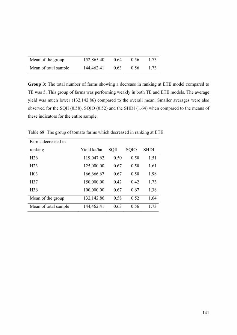
141

Mean of the group 152,865.40 0.64 0.56 1.73


Group 3: The total number of farms showing a decrease in ranking at ETE model compared to

TE was 5. This group of farms was performing weakly in both TE and ETE models. The average

yield was much lower (132,142.86) compared to the overall mean. Smaller averages were also

observed for the SQII (0.58), SQIO (0.52) and the SHDI (1.64) when compared to the means of

these indicators for the entire sample.

Table 68: The group of tomato farms which decreased in ranking at ETE

Farms decreased in


H26 119,047.62 0.50 0.50 1.51

H23 125,000.00 0.67 0.50 1.61

H03 166,666.67 0.67 0.50 1.98

H37 150,000.00 0.42 0.42 1.73

H36 100,000.00 0.67 0.67 1.38

Mean of the group 132,142.86 0.58 0.52 1.64


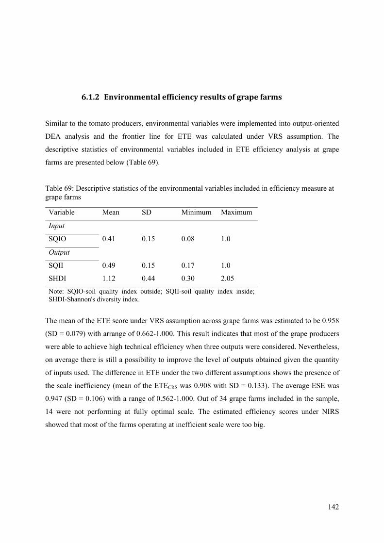
142

6.1.2 Environmentalefficiencyresultsofgrapefarms Similar to the tomato producers, environmental variables were implemented into output-oriented

DEA analysis and the frontier line for ETE was calculated under VRS assumption. The

descriptive statistics of environmental variables included in ETE efficiency analysis at grape

farms are presented below (Table 69).

Table 69: Descriptive statistics of the environmental variables included in efficiency measure at grape farms


Input

SQIO 0.41 0.15 0.08 1.0

Output

SQII 0.49 0.15 0.17 1.0

SHDI 1.12 0.44 0.30 2.05

Note: SQIO-soil quality index outside; SQII-soil quality index inside; SHDI-Shannon's diversity index.

The mean of the ETE score under VRS assumption across grape farms was estimated to be 0.958

(SD = 0.079) with arrange of 0.662-1.000. This result indicates that most of the grape producers

were able to achieve high technical efficiency when three outputs were considered. Nevertheless,

on average there is still a possibility to improve the level of outputs obtained given the quantity

of inputs used. The difference in ETE under the two different assumptions shows the presence of

the scale inefficiency (mean of the ETECRS was 0.908 with SD = 0.133). The average ESE was

0.947 (SD = 0.106) with a range of 0.562-1.000. Out of 34 grape farms included in the sample,

14 were not performing at fully optimal scale. The estimated efficiency scores under NIRS

showed that most of the farms operating at inefficient scale were too big.

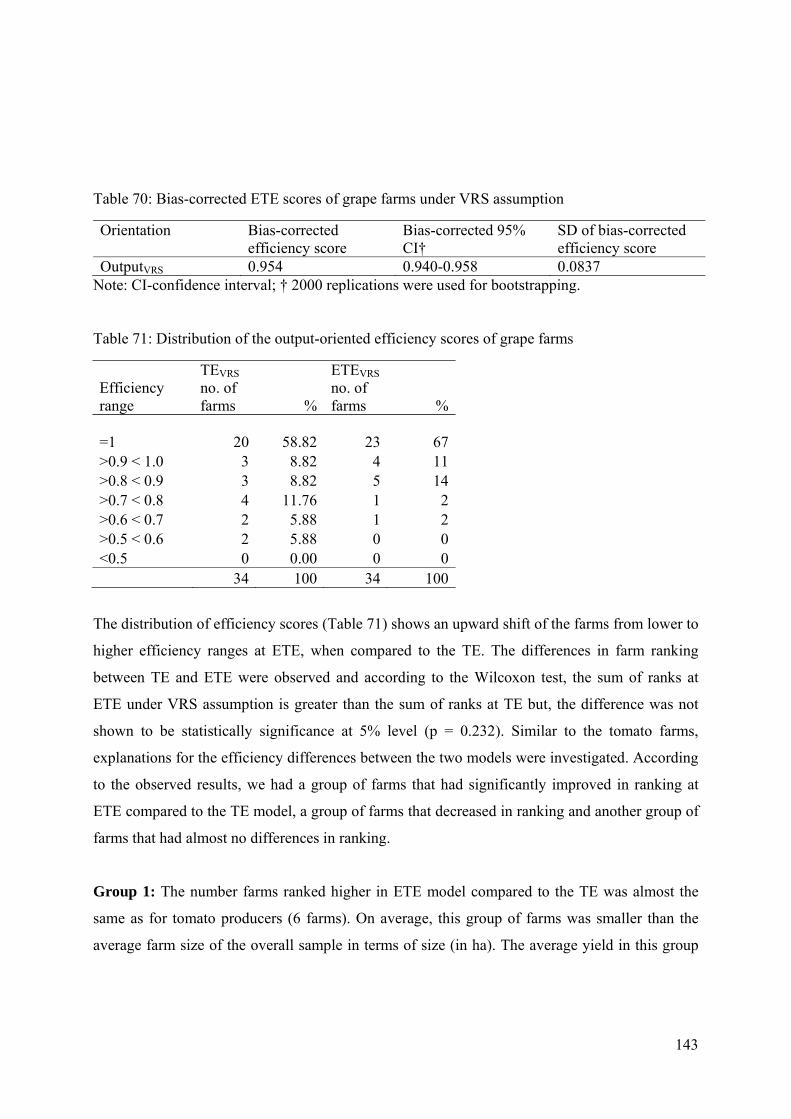
143

Table 70: Bias-corrected ETE scores of grape farms under VRS assumption




OutputVRS 0.954 0.940-0.958 0.0837 Note: CI-confidence interval; † 2000 replications were used for bootstrapping. Table 71: Distribution of the output-oriented efficiency scores of grape farms

Efficiency range



=1 20 58.82

23 67>0.9 < 1.0 3 8.82 4 11>0.8 < 0.9 3 8.82 5 14>0.7 < 0.8 4 11.76 1 2>0.6 < 0.7 2 5.88 1 2>0.5 < 0.6 2 5.88 0 0<0.5 0 0.00 0 0 34 100 34 100

The distribution of efficiency scores (Table 71) shows an upward shift of the farms from lower to

higher efficiency ranges at ETE, when compared to the TE. The differences in farm ranking

between TE and ETE were observed and according to the Wilcoxon test, the sum of ranks at

ETE under VRS assumption is greater than the sum of ranks at TE but, the difference was not

shown to be statistically significance at 5% level (p = 0.232). Similar to the tomato farms,

explanations for the efficiency differences between the two models were investigated. According

to the observed results, we had a group of farms that had significantly improved in ranking at

ETE compared to the TE model, a group of farms that decreased in ranking and another group of

farms that had almost no differences in ranking.

Group 1: The number farms ranked higher in ETE model compared to the TE was almost the

same as for tomato producers (6 farms). On average, this group of farms was smaller than the

average farm size of the overall sample in terms of size (in ha). The average yield in this group

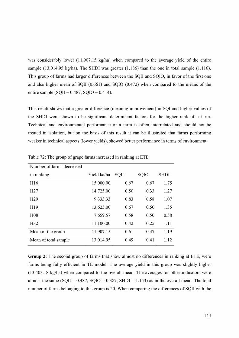
144

was considerably lower (11,907.15 kg/ha) when compared to the average yield of the entire

sample (13,014.95 kg/ha). The SHDI was greater (1.186) than the one in total sample (1.116).

This group of farms had larger differences between the SQII and SQIO, in favor of the first one

and also higher mean of SQII (0.661) and SQIO (0.472) when compared to the means of the

entire sample (SQII = 0.487, SQIO = 0.414).

This result shows that a greater difference (meaning improvement) in SQI and higher values of

the SHDI were shown to be significant determinant factors for the higher rank of a farm.

Technical and environmental performance of a farm is often interrelated and should not be

treated in isolation, but on the basis of this result it can be illustrated that farms performing

weaker in technical aspects (lower yields), showed better performance in terms of environment.

Table 72: The group of grape farms increased in ranking at ETE

Number of farms decreased

in ranking Yield ka/ha SQII SQIO SHDI

H16 15,000.00 0.67 0.67 1.75

H27 14,725.00 0.50 0.33 1.27

H29 9,333.33 0.83 0.58 1.07

H19 13,625.00 0.67 0.50 1.35

H08 7,659.57 0.58 0.50 0.58

H32 11,100.00 0.42 0.25 1.11

Mean of the group 11,907.15 0.61 0.47 1.19


Group 2: The second group of farms that show almost no differences in ranking at ETE, were

farms being fully efficient in TE model. The average yield in this group was slightly higher

(13,403.18 kg/ha) when compared to the overall mean. The averages for other indicators were

almost the same (SQII = 0.487, SQIO = 0.387, SHDI = 1.153) as in the overall mean. The total

number of farms belonging to this group is 20. When comparing the differences of SQII with the

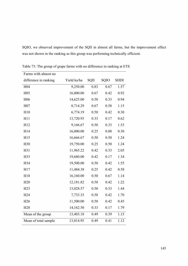
145

SQIO, we observed improvement of the SQII in almost all farms, but the improvement effect

was not shown in the ranking as this group was performing technically efficient.

Table 73: The group of grape farms with no difference in ranking at ETE

Farms with almost no

difference in ranking Yield ka/ha SQII SQIO SHDI

H04 9,250.00 0.83 0.67 1.57

H05 16,000.00 0.67 0.42 0.92

H06 14,625.00 0.58 0.33 0.94

H07 8,714.29 0.67 0.58 1.15

H10 6,774.19 0.50 0.42 0.30

H11 13,720.93 0.33 0.17 0.62

H12 9,166.67 0.50 0.33 1.53

H14 16,000.00 0.25 0.08 0.30

H15 16,666.67 0.50 0.50 1.24

H30 19,750.00 0.25 0.50 1.24

H31 11,965.22 0.42 0.33 2.05

H33 19,680.00 0.42 0.17 1.34

H34 19,500.00 0.50 0.42 1.55

H17 11,484.38 0.25 0.42 0.58

H18 16,160.00 0.50 0.67 1.14

H20 12,181.82 0.58 0.42 1.22

H23 13,028.57 0.50 0.33 1.44

H24 7,733.33 0.58 0.42 1.70

H26 11,500.00 0.58 0.42 0.45

H28 14,162.50 0.33 0.17 1.79

Mean of the group 13,403.18 0.49 0.39 1.15


146

Group 3: The third group of farms that show a decrease in ranking, consisted mostly fo farms

that had a lower average yield (12,875 kg/ha). The average SQII (0.395) has shown a decrease

when compared to the SQIO (0.437) and the SQII of the total sample. Contrary to this, the SQIO

of this group was higher than the average SQIO of the entire sample. In addition, the mean SHDI

was much lower (0.971). In summary, this group of farms had lower averages in all indicators

which is reflected in weaker performance sat TE and ETE and also a decrease in the ranking

scores.

Table 74: The group of grape farms decreased in ranking at ETE

Farms decreased in


H21 12,500.00 0.50 0.58 0.97

H02 17,142.86 0.42 0.50 0.60

H13 11,323.53 0.50 0.50 0.96

H25 16,500.00 0.42 0.25 1.19

H03 12,526.32 0.25 0.25 1.29

H01 14,042.55 0.17 0.33 1.31

H09 8,966.67 0.50 0.67 1.16

H22 10,000.00 0.42 0.42 0.30

Mean of the group 12,875.24 0.40 0.44 0.97


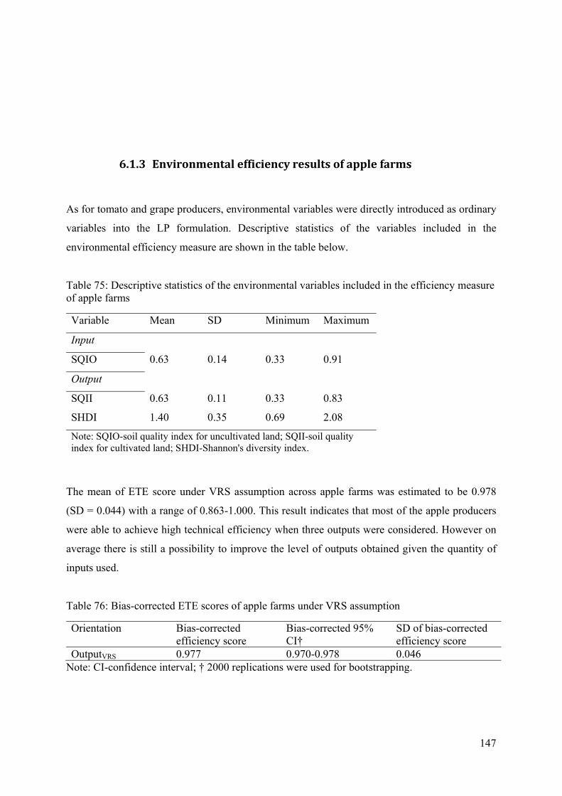
147

6.1.3 Environmentalefficiencyresultsofapplefarms

As for tomato and grape producers, environmental variables were directly introduced as ordinary

variables into the LP formulation. Descriptive statistics of the variables included in the

environmental efficiency measure are shown in the table below.

Table 75: Descriptive statistics of the environmental variables included in the efficiency measure of apple farms


Input

SQIO 0.63 0.14 0.33 0.91

Output

SQII 0.63 0.11 0.33 0.83

SHDI 1.40 0.35 0.69 2.08

Note: SQIO-soil quality index for uncultivated land; SQII-soil quality index for cultivated land; SHDI-Shannon's diversity index.

The mean of ETE score under VRS assumption across apple farms was estimated to be 0.978

(SD = 0.044) with a range of 0.863-1.000. This result indicates that most of the apple producers

were able to achieve high technical efficiency when three outputs were considered. However on

average there is still a possibility to improve the level of outputs obtained given the quantity of

inputs used.

Table 76: Bias-corrected ETE scores of apple farms under VRS assumption




OutputVRS 0.977 0.970-0.978 0.046 Note: CI-confidence interval; † 2000 replications were used for bootstrapping.

148

Table 77: Distribution of the output-oriented efficiency scores of apple farms

Efficiency range



=1 14 45.16 23 74.19>0.9 < 1.0 3 9.67 4 12.90>0.8 < 0.9 4 12.9 4 12.90>0.7 < 0.8 3 9.67 0 0>0.6 < 0.7 3 9.67 0 0>0.5 < 0.6 2 6.45 0 0<0.5 2 6.45 0 0 31 100 31 100

The distribution of efficiency scores (Table 77) shows a significant upward shift of the apple

farms from lower to higher efficiency ranges at ETE. Similar to the two other production systems

we had a group of farms that had significantly improved in ranking at ETE, a group of farms that

decreased in ranking and another group of farms that had almost no differences in ranking.

Group 1: The number farms ranked higher in ETE model was 9. The SHDI was greater (1.60)

than the one in total sample (1.41). On average the difference between SQII and SQIO was very

small (SQII = 0.61, SQIO = 0.60) and the averages were close to the ones obtained for the total

sample (SQII = 0.63, SQIO = 0.63). The average yield in this group was considerably higher

(59,156.80 kg/ha) when compared to the average yield of the total sample (54.339.35 kg/ha).

These higher values of the SHDI were shown to be significant determinant factors for the higher

rank of a farm.

149

Table 78: The group of apple farms increased in ranking at ETE

Farms improved in


H03 62,500.00 0.75 0.75 1.73

H04 55,000.00 0.50 0.67 2.09

H07 93,000.00 0.58 0.67 1.28

H12 119,615.38 0.33 0.33 1.59

H15 79,333.33 0.67 0.50 1.33

H21 45,500.00 0.75 0.58 1.84

H24 15,000.00 0.67 0.50 1.24

H06 35,062.50 0.58 0.58 1.81

H10 27,400.00 0.67 0.83 1.50

Mean of the group 59,156.80 0.61 0.60 1.60


Group 2: The second group of farms that show almost no differences in ranking at ETE, were

farms being fully efficient in TE model. The averages for SQI and SHDI were almost the same

(SQII = 0.64, SQIO = 0.66, SHDI = 1.39) as in the overall mean. The average yield in this group

was lower (46,748.41 kg/ha) when compared to the overall mean. The total number of farms

belonging to this group was 15.

150

Table 79: The group of apple farms with no difference in ranking at ETE

Farms with no

difference in ranking Yield ka/ha SQII SQIO SHDI

H05 60,416.67 0.58 0.83 0.69

H09 170,000.00 0.67 0.92 1.79

H11 83,000.00 0.58 0.42 1.60

H13 42,857.14 0.75 0.75 1.35

H14 15,000.00 0.75 0.58 1.74

H16 45,000.00 0.75 0.58 1.63

H17 45,000.00 0.42 0.75 1.28

H19 26,550.00 0.58 0.58 1.75

H20 10,920.00 0.50 0.50 1.92

H22 98,750.00 0.83 0.83 1.39

H23 35,000.00 0.42 0.42 1.04

H26 11,000.00 0.58 0.67 1.72

H29 10,000.00 0.75 0.58 1.34

H31 11,040.00 0.67 0.58 0.94

H01 36,692.31 0.75 0.83 0.75

Mean of the group 46,748.41 0.64 0.66 1.39


Group 3: Third group of farms that show decrease in ranking, were mostly farms that had

significantly higher average yield (64,411.79 kg/ha). The average SQII (0.65) showed a small

increase when compared to the SQIO (0.62). The mean of SHDI was much lower (1.16)

compared to the overall mean.

151

Table 80: The group of apple farms decreased in ranking at ETE

Farms decreased in


H27 78,666.00 0.75 0.58 1.33

H28 79,000.00 0.67 0.50 1.32

H08 123,461.54 0.67 0.83 1.38

H30 78,789.00 0.67 0.67 1.28

H34 15,900.00 0.67 0.67 0.89

H02 48,500.00 0.58 0.50 0.82

H32 26,566.00 0.58 0.58 1.08

Mean of the group 64,411.79 0.65 0.62 1.16


152

7 CONCLUSIONS

Efficiency analysis serves as bedrock for better resource utilization and policy making. The

standard efficiency measurement does not take into consideration the environmental goods and

services in the production function. Environmental externalities which are non-marketable

outputs are usually disregarded by producers in their decision making process, reflecting only

private costs and benefits. Externalities can be either negative or positive and take place when

economic entity through the production process influences the welfare of others and yet does not

pay or receive any compensation for the given effect. Positive externalities are usually

undersupplied in the market as the marginal private benefit is lower than the marginal social

benefit. Therefore, whenever positive externalities are generated policy intervention is needed to

encourage production of more positive externalities.

Agriculture plays a multifunctional role related to economic, environmental and social dimension

but it also affects other ecosystem functions such as biodiversity and soil quality. The provision

of these ecosystem functions highly depends on farmer production practices e.g. extensive

agriculture that uses less inputs (labor, fertilizers and capital) to the utilized agricultural area can

contribute to the increase of biodiversity and improve the soil quality. Rich biodiversity in

agricultural production systems contributes to the protection of ecological structure and also is in

benefit of soil conservation. Maintenance of healthy soil is not only important for production of

healthy food but it is also important for stabilization of the natural ecosystems and for better air

and water quality. Many of the conducted studies considered negative externalities generated

from agriculture into efficiency estimation. However, fewer studies were focused on positive

externalities produced by agriculture and they did not appear until the 1980s.

The overall farm household size is relatively large and it was proved to be significantly larger for

the farms oriented in tomato production when compared to apple and grape farmers. Almost all

farms included in the study were male-headed. On average farmers producing tomato were

significantly younger and considerably less educated than apple and grape farmers. The

likelihood of having additional profession aside from a farmer was proven to be dependent on

153

farmer's education. Agriculture plays an important role in the welfare of the family farms

producing tomato and it was considered to be one of the main sources of income. Family farms

producing grape choose to diversify more income sources in order to support living standards.

Whereas, different situation stands for apple producers where family farm wellbeing was mainly

based on off-farm activities. Farmer's education and the experience in terms of years active in

farming were shown to be important factors on income source determination. The household

size, number of family members working actively in farm and farm size were significantly

positively correlated with farm income.

Most of the farms are considered to be well established farms, as on average they were active in

farming for more than two decades. The average size of the farms included in the study was

considerably higher when compared to the average farm size at national level. Farm size of apple

producers was bigger followed then by grape and tomato producers. For the farmers with

primary education, the main reason of being involved in agriculture is that there was no other

opportunity for them. While, those with secondary and tertiary education 'tradition' was the most

affirmed reason. Farmers producing tomato tend to lease more land from other landowners when

compared to apple and grape producers. This is considered to be the easiest way to expand their

agriculture business without high capital investment costs. The farm land was very fragmented

for three production systems in the study and scattered over a wide area.

The soil quality index was calculated for cultivated and uncultivated farm land. Based on the

obtained results, the soil quality index of tomato farms was higher than the two other group of

farms, indicating better quality of soil for tomato producers. In general, the soil quality index at

cultivated farm land was greater when compared to the uncultivated farm land. This difference in

soil quality can be due to the effect of farm practices. The Shannon's diversity index of tomato

farms was the highest among the three groups. This shows that production systems under

perennial trees offer less possibilities to quickly change the compound and the distribution of

varieties within a given species.

154

Almost half of the total tomato farms were operating fully technically efficient under the two

different assumptions (constant and variable returns to scale) of the input oriented model. The

average technical efficiency score of tomato farms was high and there was small extent to further

reduce the level of inputs used and still obtain the same level of output produced. Choosing the

output oriented model of technical efficiency estimation, results showed that tomato producers

can further increase their output level of production by improving the resource use efficiency

given agricultural technology. Less than fifty percent of the tomato farms were operating close to

the optimal scale. The scale inefficiency of the tomato farms was mainly due to the small scale

farm.

On average grape producers used more inputs than it was needed to produce the same amount of

the output. The share of grape farms being fully efficient (under variable returns to scale

assumption at input oriented model) was over fifty percent. At the output oriented model

(variable returns to scale assumption), grape producers on average could have increased the level

of output by ten percent and still keep the same level of inputs used. Most of the grape farms

were operating at relatively high optimal scale. The estimated results under non-increasing

returns to scale showed that scale inefficiency was mainly present of small holder farms.

The share of apple farms being fully technical efficient under variable returns to scale

assumption was less than fifty percent. This result indicates that apple producers on average

could have reduced the amount of inputs used given the level of output produced. When output

oriented model under variable returns to scale assumption was performed, the results showed that

on average apple farms could produce fifteen percent more of the output, using the same quantity

of inputs. The level of fully scale efficient farms producing apple was considerably smaller when

compared to the two other groups of farms. Similar to tomato and grape producers, for majority

of the apple producers the inefficiency scale was present due to being too small farms.

At the estimation of environmental efficiency, the output oriented model under the variable

returns to scale assumption was extended by adding up two additional variables that signified

155

soil quality of the farm land and agro-biodiversity provision by each production system

considered in the study. In DEA the efficiency score increases when additional inputs or outputs

are introduced into the model. Therefore, at the environmental efficiency estimation farm

efficiency scores were in general higher when were directly compared to the technical efficiency

scores of the output oriented model.

As the environmental efficiency and technical efficiency models were not constituting similar

production function, a direct comparison between environmental and technical efficiency scores

for each farm was not appropriate. As a result, the differences in ranking between the two models

were observed. Three different groups in terms of positioning in ranking were found. The first

group consisted of farms which showed an increase in ranking at environmental efficiency when

compared to the technical one. In the second group, were farms that did not show differences in

ranking and in the third group were farms that decreased in ranking at environmental efficiency

when compared to the technical efficiency estimation.

Farms which showed increase in ranking at environmental efficiency estimation, were mostly

those that improved or maintained good level of soil quality and had a high value of Shanno's

diversity index. The second group of farms that did not show difference in ranking, were fully

efficient in environmental and technical efficiency estimation. That is why it was not possible to

distinguish the inclusion effect of environmental factors into the efficiency estimation. The third

group of farms were performing weakly in both, technical and environmental efficiency

estimation. In general, for this group of farms, smaller averages were observed for the soil

quality index and the Shannon's diversity index when compared to the averages of total sample.

Based on the study results smaller farms in terms of UAA seemed to stand better at estimated

environmental efficiency. However, further research is needed in order to bring more evidence

and knowledge associated to environmental performance of farms by size. The inclusion of more

indicators from agro-ecological and socio-territorial scale will provide broader picture for more

sustainable farming systems.

156

Environmental efficiency estimation is completely new approach in Kosovo and it can serve as a

good base for further research towards environmental and sustainability performance of farms. It

will be particularly important for smaller farms as they were usually excluded from the policy

support and by considering other dimensions into efficiency estimation the support given to them

might be justified. The results of the efficiency analysis in the study can serve as model for the

development of evidence based policies.

157

WorksCitedAdler N., F. L.-S. (2002). Review of ranking methods in the data envelopment analysis context.

European Journal of Operational Research 140 (2002) 249–265 .

Ali I. A., and Seiford M. L. (1990). Translation invariance in Data Envelopment Analysis.

Operations Research Letters 9 (1990) 403-405 .

Amacher M. C., O. P. (2007). Soil vital signs: a new soil quality index (SQI) for assessing forest

soil health. Forest Service-United Stated Department of Agriculture.

Amacher, M. C. (2007). Soil Vital Signs : A New Soil Quality Index (SQI) for Assessing Forest

Soil Helath. US: Rocky Mountain Research Station.

Anderesn P., and Petersen N. (1993). A procedure for ranking efficient units in Data

Envelopment Analysis. Management Science 39 (10): 1261-1264 ,

http://pubsonline.informs.org/doi/pdf/10.1287/mnsc.39.10.1261.

Antonio F. Amores F.A. and Contreras I. (2009). New approach for the assignment of new

European agricultural subsidies using scores from data envelopment analysis: Application to

olive-growing farms in Andalusia (Spain). European Journal of Operational Research 193

(2009) 718–729 , www.elsevier.com/locate/ejor.

Armsworth P. R., K. B. (2004). An introduction to biodiversity concepts for environmental

economists. Resource and Energy Economics , pp. 115-136.

Arovuori, K. (2008). Controversies between Stated Agricultural Policy Objectives and Policy

Measures in the EU's CAP. 12th Congress of the European Association of Agricultural

Economists-EAAE 2008 , http://ageconsearch.umn.edu/bitstream/43844/2/620.pdf.

158

Arovuori, K. (2008). Controversies between Stated Agricultural Policy Objectives and Policy

Measures in the EU's CAP. 12th Congress of the European Association of Agricultural

Economists - EAAE. Ghent-Belgim.

Aswathanarayana, U. (2012). Natural Resources: Technology, Economics and Policy. Taylor &

Francis Group, LLC: eBook-PDF.

B. F. (1958, August). The Anatomy of Market Failure. The Quarterly Journal of Economics,

Vol.72, No.3, in MIT Press http://opim.wharton.upenn.edu/~sok/papers/b/Bator-market-

failure.pdf , pp. 351-379.

Balmford A., B. A. (2002). Economic reasons for conserving wild nature. Science , pp.950-953.

Banker RD., C. A. (1984). Some Models for Estimating Technical and Scale Inefficiencies in

Data Envelopment Analysis. Management Science 30 (9) , 1078-1092.

Barbier E. B. (2007). Valuing ecosystem services as productive inputs. Economic Policy 22(49):

177–229. , http://earthtek.org/EVPP524/ProdFunc_Barbier2007EP.pdf.

Barnes A.P. (2006). Does multi-functionality affect technical efficiency? A non-parametric

analysis of the Scottish dairy industry. Journal of Environmental Management 80:287-294 .

Baumgärter, S. (2005, September 5). Measuring the diversity of what? and for what? A

conceptual comparison of ecological and economic biodiversity indices. Department of

Economics, Univeristy of Heidelberg, Germany .

Beaufoy G. (2007). HNV Farming-Explaining the Concept and Interpreting EU and National

Policy Commitments. European Forum on Nature Conservation and Pastoralism .

159

Blandford D. (2011). The Contribution of Agriculture to Green Growth. Pennsylvania State

University, University Park, PA 16802, United States: Professor of Agricultural and

Environmental Economics. https://www.oecd.org/tad/sustainable-agriculture/48258861.pdf.

Boussofiane A., D. R. (1991). Applied Data Envelopment Analysis. European Journal of

Operational Research 52 (1991) 1-15 .

Bowlin, W. (1998). Measuring Performance: An Introduction to Data Envelopment Analysis

(DEA). Journal of Cost Analysis .

Brander L., G.-B. E.-L. (2010). The economics of valuing ecosistem serrvices and biodiversity.

The Ecological and Economic Foundations.

Brander L., Gómez-Baggethun E., Martín-López B., Verma M. (2010). The Economics of

Ecosystems and Biodiversity: The Ecological and Economic Foundations. London and

Washington: Pushpam Kumar, Earthscan.

Bytyqi, H., Vegara, M., Gjonbalaj, M., Mehmeti, H., Gjergjizi, H., Miftari, I., et al. (2008).

Analysis of Consumer Behavior in Regard to Dairy Products in Kosovo. J.Agric.Res .

Callicot, J. C. (1999). Current normative concepts in conservation. Conservation Biology , 13:

23-24.

Charnes A., C. W. (1985). Foundations of Data Envelopment Analaysis for Pareto-Koopmans

efficient empirical production functions. Journal of Econometrics 30 (1985) 91-107. North

Holland.

Charnes, A. C. (1978). Measuring the efficiency of decision-making units. European Journal of

Operational Research , 429-444.

160

Charnes, A. W., & al., e. (1978). Measuring the infficiency of cecision making units. European

Journal of Operational Research , 429-444.

Chen Q., S. T. (2014). Assessment of Agri-Environmental Externalities at Regional Levels in

Finland. Sustainability 2014, 6, 3171-3191; doi:10.3390/su6063171 .

Chung H. Y., Färe R. and Grosskopf S. (1997). Productivity and Undesirable Outputs: A

Directional Distance Function Approach. Journal of Environmental Management (1997) 51,

229–240 .

Clawson M. (1959). Methods of measuring the demand and value of outdoor recreation. In:

Mendelsohn R. & Olmstead S., 2009.he Economic Valuation of Environmental Amenities and

Disamenities: Methods and Applications.Annual Reviews.School of Forestry and Environmental

Studies,. Washington, DC: Resour. Future, Reprint 10.

Coelli T., R. S. (2002). Technical, Allocative, Cost and Scale Efficiencies in Bangladesh Rice

Cultivation: A Non-parametric Approach. Journal of Agricultural Economics , 53 (2002): 607-

26.

Coelli, T. P. (2005). "An Introduction to efficiency and Productivity Analysis", 2nd Edition. New

York, USA: Springer Science & Business Media, Inc.

Coelli, T. (1995). Recent Developments in Frontier Modeling and Efficiency Measurement.

Australian Journal of Agricultural Economics , 219-45.

Cook D.W., and Zhu J. (2015). Data Envelopment Analysis. Ch.2: DEA Cross Efficiency. New

York: Springer Science+Business Media. International Series in Operations Research &

Management Science 221, DOI 10.1007/978-1-4899-7553-9_2.

161

Cooper J. C. (2001). The environmental roles of agriculture: economic valuation of the

environmental externalities of agriculture. Rome, Italy March19 to 21, 2001: 31–88.

Expert Meeting Proceedings: First Expert Meeting on the Documentation and Measurement of

the Roles of Agriculture in Developing Countries.

Cooper T., H. K. (2009). Provision of Public Goods through Agriculture in the European Union.

Institute for European Environmental Policy.

Cooper W W., S. L. (2000). Data envelopment analysis: a comprehensive text with models,

references and DEA-Solver Software applications. Boston: Kluwer Academic Publishers.

Cooper W. W., L. M. (2011). Handbook on Data Envelopment Analysis. Chapter 2: Returns to

Scale in DEA. International Series in Operations Research & Management Science 164, Springer

Science+Business Media, LLC 2011.

Cooper W., S. L. (2002). Data Envelopment Analysis. A comprehensive Text with Models,

Applications, References and DEA Solver Software. New York, Boston, Dordrecht, London,

Moscow: Kluwer Academic Publishers.

Cooper WW., P. K. (2001). IDEA (Imprecise Data Envelopment Analysis) with SMDs (Column

Maximum Decision Making Units). Journal of the Operational Research Society (2001) 52, 176-

181 , https://www.jstor.org/stable/pdf/254145.pdf.

Daily G. C., A. S., & et al, ,. D. (1997). Ecosystem Services: benefits supplied to human societies

by natural ecosystems. Issues in Ecology (2).

Daly, E. H. (1992). Steady-State Economics: Concepts, Questions, Policies. Ecological

Economics No.6 pp.333-338 .

162

Debreu G. (1951). The coefficient of resource utilization. Econometrica , 19 (3): 273-292.

Debreu, G. (1951). The coefficient of resource utilization. Econometrica 19 (3): 273-292 .

Di Falco S., and Perrings C. (2005). Crop biodiversity, risk management and the implications of

agricultural assistance. Ecological Economics , pp. 459-446.

Dixon J., Pagiola S. (1998). Economic Analysis and Environmental Assessment. Environmental

Economics and Indicators Unit, Environment Department.

Doyle J., and Green R. (1994). Efficiency and Cross-efficiency in DEA: Derivations, Meanings

and Uses. Journal of Operational Research Society. Vol.45, No.5, pp.567-578 .

EC. (2013). Overview of CAP Reform 2014-2020. Available at:

http://ec.europa.eu/agriculture/policy-perspectives/policy-briefs/05_en.pdf.

Egner, H., Riehm, H., & Domingo, W. (1960). Untersuchungen uber die chemische

Bodenanalyse als Grunlage fur die Beurteilung des Nahrstoffzustandes der Boden II. Chemische

Extractionsmethoden zu Phosphor un Kaliumbestimmung. K. Lantbr. Hogsk. Annlr. W.R. 26:

199-215.

Elezi Xh., Zogaj M., Halimi A. . (2004b). Bazat e shkencës së tokës II. Material intern për

student. Fakulteti i Bujqësisë dhe Veterinarisë-Universiteti i Prishtinës "Hasan Prishtina":

Prishtinë.

Elezi, X., Halimi, A., & Zogaj, M. (2004a). Digitization of Kosovo's pedological map (in

Albanian). Prishtine: Chair of Soil Scince at Agriculture and Veterinary Faculty-University of

Prishtina "Hasan Prishtina".

163

Erjavec, E., & Dimitrievski, D. (2008). EU Common Agricultural Policy and Accession Tasks

for Western Balkan's Countires. Skopje: Faculty of Agricultural Sciences and Food.

Estudillo, J. O., & Otsuka, E. (2010). Rural poverty and income dynamics in southeast Asia.

Norrthe Holland-Amsterdam: In: Evenson, R., Pingali, P., Handbook of Agricultural Economics.

FAO. (2010). From payment of environmental externalities to remuneration of positive

externalities in the agriculture and food sector. Rome: FAO.

FAO. (1999). Taking stock of the multifunctional character of agriculture and land. Paper for

FAO/Netherlands Conference on the Multifunctional character of Agriculture and Land.

Maastricht, The Netherlands September 12–19, 1999.

FAO. (2001). The Environmental Roles of Agriculture, Summary Report for First Expert

Meeting on the Documentation and Measurement of the Roles of Agriculture in Developing

Countries, Rome, Italy March19 to 21, 2001. Rome, Italy: FAO.

Färe R. and Grosskopf S. (2004). Modeling undesirable factors in efficiency evaluation:

Comment. European Journal of Operational Research 157 (2004) 242–245 .

Färe, R. G., & Roos, F. G. (1998). "Malmquist productivity indexes: a survey of theory and

practice", in Coelli, T.J., Prasada Rao, D.S. O'Donnell, C.J and Battese,G.E (2005) "An

Introduction to efficiency and Productivity Analysis", 2nd Edition. New York, USA: Springer

Science & Business Media, Inc.

Farrell, M. (1957). The Measurement of Production Efficiency. Journal of the Royal Statistical

Society , 253-90.

164

Feather P., H. D. (1999). Economic Valuation of Environmental Benefits and the Targeting of

Conservation Programs. Economic Research Service/USDA.

Fischer Ch. (2004). Assesing Kosovo's horticultural potential-the market for fruits and

vegetables on the Balkans. Institute of Agricultural Development in Central and Eastern Europe

, http://ageconsearch.umn.edu/bitstream/92025/2/dp67.pdf.

Fisher B., and Turner R. K. (2008). Ecosystem Services: clasification for valuation. Biological

Conservation , 1167-1169.

Fisher B., B. I. (2011). Valuing ecosystem services: Benefits, Values, Space and Times.

Environment for Development .

Garrod, G. W. (1999). Economic Valuation of the environment. In:Brander L., Gómez-

Baggethun E., Martín-López B., Verma M. 2010.The Economics of Ecosystems and Biodiversity:

The Ecological and Economic Foundations.Pushpam Kumar, Earthscan. London and

Washington DC. Cheltenham: Edward Elgar.

Gjonbalaj, M., Miftari, I., Pllana, M., Fetahu, S., Bytyqi, H., Gjergjizi, H., et al. (2009,

December Zagreb). Analyses of Consumer Behavior and Wine Market in Kosovo. Agriculturae

Conceptus Scientificus , pp. Vol. 74, No. 4 (333:338)

http://www.agr.unizg.hr/smotra/pdf_74/acs74_58.pdf.

Glanz AA. (1995). Saving Our Soil: Solutions for Sustaining Earth's Vital Resource. In: Masto

R.E et al. (2008) Soil quality indices for evaluation of long term land use and soil management

practices in semi-arid sub-tropical india. Land Degradation and Development. Johnson Books.

165

Gomes EG., and Lins MPE. (2007). Modelling undesirable outputs with zero sum gains data

envelopment analysismodels. Journal of the Operational Research Society , www.palgrave-

journals.com/jors.

Greene H.W. (2003). Econometric Analysis. New Jersey: Pearson education, Inc.

Greene, W. H. (1997). Frontier production functions, In Francesco Porcelli: Measurement of

Technical Efficiency. A brief survey on parametric and non-parametric techniques.

Gregorich E., C. M. (1993). Towards a minimum data set to assess soil organic matterquality in

agricultural soils. Canadian Journal of Soil Science .

Grosskopf, S. (1985). The Measurement of Efficiency of Production. Kluwer-Nijholff Publishing,

USA .

Hayo M.G. van der Werf and Petit J. (2002). Evaluation of the environmental impact of

agriculture at the farm level: a comparison and analysis of 12 indicator-based methods.

Agriculture, Ecosystems and Environment 93 (2002) 131–145 , www.elsevier.com/locate/agee.

Heal G.M., E. B. (2005). Valuing Ecosystem Services: Toward Better Environmentla Decision

Making. In: Barbier E. B, 2007. Valuing ecosystem services as productive inputs.Economic

Policy 22(49): 177–229. Washington DC: The National Academics Press.

Helm, D. (1988). Theoretical Concepts and Criteria of Appraisal. Consortia Paper One.

Electricity Industry Task Froce, Willington.

Hill, B. (2012). Understanding the Common Agricultural Policy. USA and Canada: Earthscan.

Hill, B. (2012). Understanding the Common Agricultural Policy. London: Earthscan.

166

Hodgson G. (1999). ECONOMICS AND UTOPIA Why the learning economy is not the end of

history. 11 New Fetter Lane, London EC4P 4EE: Routledge.

Imami D. (2016). Agriculture value chain analysis in Kosovo. Prishtine: MAFRD-FAO.

Jollands N. (2006). Concepts of efficiency in ecological economics: Sisyphus and the decision

maker. Ecological Economics 56 (359-372) , www.elsevier.com/locate/ecolecon.

Jollands, N. (2003). An Ecological Economics of Eco-Efficiency: Theory, Interpretations and

Applications to New Zeland. Massey University, PhD thesis.

Just R., H. D. (2004). The welfare economics of public policy. Northampton, Massachusetts

USA: Edward Elgar Publishing, Inc.

Karimov A. (2013). Productive Efficiency of Potato and Melon Growing Farms in Uzbekistan: A

Two Stage Double Bootstrao Data Envelopment Analysis. Agriculture , 3 (2013) 503-515.

KAS. (2013). Agricultural input price indices. Kosovo Agency of Statistics .

KAS. (2013). Agricultural output price indices. Kosovo Agency of Statistics .

KAS. (2013). External Trade Statistics; Agro-food trade data according to Combine

Nomenclature of Custom Tariffs (CNCT 1-24). Kosovo Agency of Statistics .

KAS. (2013). External Trade Statistics; Agro-food trade data according to Combine

Nomenclature of Custom Tariffs (CNCT 1-24). Kosovo Agency of Statistics .

KAS. (2014). Statistical Yearbook of the Republic of Kosovo. Prishtinë.

167

Kelly E., S. L. (2012). Application of data envelopment analysis to measure technical efficiency

on a sample of dairy farms. Irish Journal of Agricultural and Food Research 51: 63-77 .

Kerry-Turner, R. (2004). Environmental and ecological economics perspectives. In: Biodiversity

and ecosystem services in agricultural landscapes- are we asking the right questions? Agriculture

Ecosystems & Environment .

Kleijn, D. B. (2008). In research for key biogeochemical factors affecting plant species

persistence in heathland and acidic grasslands: a comparison of common and rare spcies. Journal

of Applied Ecology , 680-687.

Kontoleon A., P. U. (2007). Biodiversity Economics: Principles, Methods and Applications.

In:Brander L., Gómez-Baggethun E., Martín-López B., Verma M. 2010.The Economics of

Ecosystems and Biodiversity: The Ecological and Economic Foundations. Pushpam Kumar,

Earthscan. London: Cambridge University Press, pp.343-368.

Koopmans, T. (1951). An analysis of production as an efficient combination of activities. In T.C.

Koopmans (ed) Activity Analysis of production and allocation. New York. John Wiley and sons,

Inc.: Cowles Commission ofr Resarch in Economics. Monograph 13.

Koopmans, T. C. (1951). 'An Analysis of Production as an Efficient Combination of Activities,'

In, T.C Koopmans (ed.) Activity Analysis of Production and Allocation. New York & London:

John Wiley & Sons; Chapman & Hall, Limmited.

Kortelainen M., and Kuosmanen T. (2004). Measuring eco-efficiency of production a frontier

approach. Department of Business and Economics, University of Joensuu and Environmental

Economics and Natural Resources Group, Wageningen University .

168

Kriström B. (1990). Valuing environmental benefits using the contingent valuation method.

Sweden: Umeå Economic Studies No.291-University of Umeå.

Kuosmanen T. & Kortelainen M. (2004). Data envelopment analysis in environmental valuation:

environmental performance, eco-efficiency and cost-benefit analysis.

Kuosmanen T. (2005). Measurement and Analysis of Eco-efficiency-An Economist's

Perspective. Journal of Industrial Ecology V. 9. No.4 .

Kuosmanen T. (2005). Weak disposability in nonparametric production analysis with undesirable

outputs. American Journal of Agricultural Economics 87 (4) (November 2005):1077-1082 .

Kuosmanen T., B. N. (2009). Environmental cost–benefit analysis of alternative timing strategies

in greenhouse gas abatement: A data envelopment analysis approach. Ecological Economics 68

(2009) 1633-1642 .

Leibenstein, H. (1966, June Volume 56, Issue 3, 392-415). Allocative Efficiency vs. "X-

Efficiency". The American Economic Review .

Lertworasirikul S., F. S.-C. (2003). Fuzzy data envelopment analysis (DEA): a possibility . Fuzzy

Sets and Systems 139 (2003) 379–394 .

Lévéque C., & Mounolou J. C. (2003). Biodiversity. London: John Wily & Sons, Ltd.

Lovell K., and Pastor J. (1995). Units invariant and translation invariant DEA models.

Operations Research Letters 18 (1995) 147-151 .

M., Kuosmanen T. & Kortelainen. (2006). Valuing Environmental Factors in Cost-Benefit

Analysis Using Data Envelopment Analysis. The Fondazione Eni Enrico Mattei ,

http://www.feem.it/Feem/Pub/Publications/WPapers/default.htm.

169

MAFRD. (2010). Agriculture and Rrual Development Program 2007-2013. Prishtine.

MAFRD. (2013). Agriculture and Rural Development Program 2014-2020. Prishtine.

MAFRD. (2013). Green Report 2012. Ministry of Agriculture Forestry and Rural Development .

MAFRD. (2014). Green Report 2013. Prishtine: Ministry of Agriculture Forestry and Rural

Development.

MAFRD. (2014). Green Report 2013. Ministry of Agriculture Foresty and Rural Development .

MAFRD. (2013). Green Report Kosovo 2013. Prishtinë: Ministry of Agriculture Forestry and

Rural Development.

MAFRD. (2013). Horticultural strategy of Kosovo 2009-2013. Prishtine: MAFRD.

MAFRD. (2003). Kosovo Gren Book-Agriculture and Rural Sustainable Development Strategy

in Kosovo. Prishtine.

MAFRD. (2012). Mid-Term Evaluation Report of the ARDP 2007-2013. Prishtine.

Magurran, A. (2004). Measuring Biological Diversity. Blackwell Science Ltd: UK.

Magurran, A. (2004). Measuring Biological Diversity. Blackwell Science Ltd: UK.

Manjunathaa A.V., A. R. (2012). Impact of land fragmentation, farm size, land ownership and

crop diversity on profit and efficiency of irrigated farms in India. Land Use Policy .

170

Mankiw G. (2000). Principles of Microeconomics 2nd Edition. Harcourt College Pub.

Mankiw, N. G. (2007). Principles of Microeconomics 4th Edition. Thomson South Western.

Masterson T. (2007). Productivity, Technical Efficiency, and Farm Size in Paraguayan

Agriculture. Working Paper No. 490 of the Levy Economics Institute of Bard College .

Masto R.E., C. P. (2008). Soil quality indices for evaluation of long term land use and soil

management practices in semi-arid and sub-tropical India . Land Degradation & Delopment .

Mbaga-Zemgawale Z., and Folmer H. (2000). Household adoption behaviour of improved soil

conservation: The case of North Pare and West Usambara Mountains of Tanzania. Land Use

Policy , 17 (4): 321-36.

McGarical K., Marks B. J. (1995). FRAGSTATS: Spatial Pattern analysis program for

quantifying landscape structure. Portland, OR, USA: USDA Forest Services.

Mendelsohn R. & Olmstead S. (2009). The Economic Valuation of Environmental Amenities and

Disamenities: Methods and Applications. School of Forestry and Environmental Studies, Yale

University, New Haven: Annual Reviews.

Miettinen, A. L.-K. (2004). On diversity effects of alternative agricultural policy reforms in

Finland: An agricultural sector modeling approach. Agricultural and Food Science , pp.229-246.

Miftari, I. &., & Gjonbalaj, M. (2013). Farm Diversification and alternative activities in rural

areas in Kosovo. Prishtine: On behalf of the GIZ project: Rural Economic Development (RED)

in Kosovo (PN: 09.2289.8_001.00).

Moschini, G. H., & Hennessy, M. (2001). Handbook of Agricultural Economics. Elsevier.

171

Müller F., D. G. (2010). Ecosystem services at the landscape scale: the need for integrative

approches. Landscape Online .

Mulugeta E. (2013). An economic valuation of biodiversity and livestock. NUI Galway

http://hdl.handle.net/10379/3400.

Noss F. R. . (1990). Indicators for Monitoring Biodiversity: A Hierarchical Approach.

Conservation Biology .

Nowak A., K. T. (2015). Technical efficiency and its determinants in the European Union

agriculture. Agric.Econ – Czech, 61, 2015 (6): 275–283 .

Oates W. & Portney P. (2003). The political economy of environmentla policy. Department of

Economics, University of Maryland, College Park, MD, and Resources for the Future :

Washington, DC, USA.

O'Rourke E. and Kramm N. (2012). High Nature Value (HNV) farming and the management of

upland diversity-a review. European Countryside , 2 (2012) 116-133.

Ortner K., H. J. (2006). The efficiency of dairy farms in Austria - do natural conditions matter?,

(pp. 96th EAAE-Sem. 1/2006). Tänikon, CH.

Pacini C., W. A. (2003). Evaluation of sustainability of organic, integrated and conventional

farming systems: farm and field-scale. Agriculture Ecosystems and Environment .

Padilla-Fernandez M. D., and Nuthall L. P. (2009). Technical efficiency in the production of

sugar cane in Cerntral Negros area, Philippines: An application of Data Envelopment Analysis.

J. ISSAAS Vol.15 No. 1: 77-90 (2009) .

172

Pattanayak S. & Kramer R. (2001). Worth of watersheds: a producer surplus approach for

valuing drought mitigation in Eastern Indonesia. Environment and Development Economics ,

http://dukespace.lib.duke.edu/dspace/bitstream/handle/10161/6747/Pattan-

Kramer_Worth_Watersheds_EDE_2001.pdf?sequence=1.

Patterson, M. G. (1996). What is energy efficiency? Concepts, indicators and methodological

issues. Energy Policy .

Pearce D. & Barbier E. (2000). Blueprint for a Sustainable Economy, In: Holder J. and Lee M.,

2007, Environmental Protection, Law and Policy 2nd Edition, Cambridge University Press, New

York, USA. London: Earthscan.

Pearce R. K., Turner D. W. (1990). Economics of natural resources and the environment.

Harvester Wheatsheaf.

Porcelli F. (2009). Measurement of technical efficiency: A brief survey on parametric and non-

parametric techniques.

Reinhard S., L. K. (1999). Econometric estimation of technical and environmental efficiency: an

application to Dutch dairy farms. American Journal of Agricultural Economics, Vol. 81, No. 1

(Feb., 1999), pp. 44-60 .

Revesz R. & Stavins R. (2004). Environmental Law and Public Policy. Resources for the future:

Discussion paper 04-03. rev .

Rutherford D. (2007). ECONOMICS-The key concepts. London and New York: Routledge.

173

Sauer J., Gorton M., Davidova S. (2014). Migration and Agricultural Efficiency: evidence from

Kosovo. Selected Paper prepared for presentation at the Agricultural & Applied Economics

Association’s 2014 .

Schader Ch. (2009). Cost-effectiveness of organic farming for achieving environmental policy

targets in Zwitzerland. Zwitzerland: Research Institute of Organic Agriculture (FiBL).

Scheel H. (2001). Undesirbale outputs in efficiency valuations. European Journal of Operational

Research 132 (2001) 400-410 .

Seiford M. L., and Zhu J. (2002). Modeling undesirable factors in efficiency evaluation.

European Journal of Operational Research142 (2002) 16–20 .

Simar L., and Wilson W. P. (2007). Estimation and inference in two-stage, semi-parametric

models of production processes. Journal of Econometrics 136 (2007) 31–64 .

Simpson, J., & Weiner, E. (1989). The Oxford English Dictionary. Oxford: Clarendon Press.

Sipiläinen T., and Huhtala A. (2011). Opportunity costs of providing crop diversity inorganic

and conventional farming: would targeted environmentl policies make economic sense? EAAE

Congress: Change and Uncertainty Challenges for Agriculture, Food and Natural Resources.

Zurich, Switzerland.

Sipiläinen T., M. P.-O. (2008). Efficiency in Agricultural production of biodiversity: organic vs

conventional practices. EAAE Seminar "Modeling of Agricultural and Rural Development

Policies. Sevilla, Spain.

Sipiläinen T., Marklund P., Huhtala A. (2008). Efficiency in agricultural production of

biodiversity: organic vs. conventional practices. Paper prepared for presentation at the 107th

174

EAAE Seminar "Modeling of Agricultural and Rural Development Policies". Sevilla, Spain,

January 29th -February 1st, 2008 .

Skeat, W. (1961). An Etymological Dictionary of the English Language. Clarendon Press,

Oxford.

SoCo. (2009). Final report on the project 'Sustainable agriculture and soil conservation' . JRC

Scientific and Technical Reports.

Soda O. (2003). Nogaku Genron. Translated by Y. Zhang Chinese ed. China Renmin University

Press, Baijing (in Chinese). In: Yao Lv, Shu-zhong Gu, Dong-mei Guo, 2010,Valuing

environmental externalities from rice–wheat farming in the lower reaches of the Yangtze River.

Ecological Econimics, 69 (2010) 1436–1442.

Solovyeva I. and Nuppenau A. E. (2013). Environmental Efficiency of Traditional Farming with

Consideration of Grassland Biodiversity: Implication for the Ukrainian Carpathians . 87th

Annual Conference of the Agricultural Economics Society, University of Warwick, United

Kingdom .

Solovyeva I., and Nuppenau E. A. (2012). Improving Measures for Targeting Agri-

Environmental Payments: The Case of High Nature Value Farming. European Association of

Agricultural Economists, 126th Seminar, Capri, Italy, 27-29 June, 2012, AgEconSearch .

Spornberger, A., Kullaj, E., Mehmeti, A., Ohlinger, B., Sylana, S., Demaj, D., et al. (2014).

Organic apple growing in Kosovo and Albania-a survey of the current situation and possibilities

for improvement.

175

Stavins R. (2004). Introduction to the Political Economy of Environmental Regulation. KSG

Faculty Research Working Paper Series. John F. Kennedy School of Government & Harvard

University .

Stein, J. G. (2001). The Cult of Efficiency. House of Anansi Press. Canada: www.anansi.ca.

Swift M.J, A.-M. I. (2004). Biodiversity and ecosystem services in agriculture landscapes- are

we asking the right questions. Agriculture Ecosystems & Environment .

Swift, M. V. (1996). Biodiversity and agroecosystem function. In: Cushman, J.H., Mooney,

H.A., Medina, E., Sala, O.E., Schulze, E.D. Functional Roles of Biodiversity: A Global

Perspective. Wiley, Chichester, pp.261-298.

Szenberg M. & Ramrattan L. (2004). New Frontiers in Economics. New York, USA: Cambridge

University Press. Taking stock of the multifunctional character of agriculture and land. Paper.

(n.d.).

Thanassoulis, E. (2001). Introduction to the theory and application of data envelopment

analysis: a foundation text with integrated software. Boston: Kluwer Academic Publisher.

Toloo M, and Nalchigar S. (2009). A new integrated DEA model for finding most BCC-efficient

DMU. Applied Mathematical Modelling 33 (2009) 597–604 ,

http://www.sciencedirect.com/science/article/pii/S0307904X08000395.

Toloo M., S. B. (2009). A new method for ranking discovered rules from data mining by DEA.

Expert Systems with Applications ,

http://www.sciencedirect.com/science/article/pii/S0957417408007586.

176

Tone K. (2001). A slacks-based measure of efficiency in data envelopment analysis. European

Journal of Operational Research .

Tyteca D. (2006). On the Measurement of the Environmental Performance of Firms—A

Literature Review and a Productive Efficiency Perspective. Journal of Environmental

Management (1996) 46, 281–308 .

UNEP. (1992). Convention on Biological Diversity.

Vandermeer J., N. M. (1998). Global change and and multi-species agroecosystems: Concpets

and issues. Agriculture Ecosystems & Environment .

Volk, T. (2010). Agriculture in the Western Balkan Countries. Leibniz Institute of Agricultural

Development in Central and Eastern Europe IAMO: Halle.

Volk, T., Rednak, M., Erjavec, E., & Juvančič, L. (2012). Development of a tool for comparative

analysis of agricultural and rural development policies measures and its application on Western

Balkan countries. Selected Poster prepared for presentation at the International Association of

Agricultural Economists (IAAE) Triennial Conference, Foz do Iguaçu, Brazil, 18-24 August,

2012 , http://ageconsearch.umn.edu/bitstream/126918/2/Juvan%c4%8di%c4%8d.pdf.

Vuçitërna R., T. R. (2017). Efficiency and Competitiveness of Kosovo Raspberry Producers.

Selected Paper prepared for presentation at the Southern Agricultural Economics Association’s

2017 Annual Meeting, Mobile, Alabama, February 4-February 7, 2017 .

Waldhardt R. et al. (2010). Evaluating Today's Landscape Multifunctionality and Providing an

Alternative Future: A Normative Scenario Approach. Ecology and Society ,

http://www.ecologyandsociety.org/vol15/iss3/art30/.

177

Waldhardt R., and Otte A. . (2003). Indikation floristischer Diversität in Agrarlandschaften über

Habitatmuster und deren Altersstruktur. Schr.reihe agrarspectrum 36: 199-205.

Wanke P., B. C. (2016). Assessing productive efficiency of banks using integrated Fuzzy-DEA

and bootstapping: A case of Mozambican banks. European Journal of Operational Research ,

249 (2016) 378-389.

Wehinger, T., & Zhllima, W. (2013). Sector Analysis for the diversification of the rural Economi

in Albania. Tirana: UN0 FAO on the request of the Minister for Agriculture, Rural Development

and Water Administration (MARDWA) of the Republic of Albania.

Wellstein C., Otte A., and Waldhardt R. (2007). Impact of site and management on the diversity

of Central European mesic grassland. Agriculture, Ecosystems and Environment .

Wilson, E. O. (1988). The diversity of life. Cambridge: Harvard University Press.

Young RA. (2005). Determining the Economic Value of Water: Concepts and Methods. In:

Mendelsohn R. & Olmstead S., 2009. The Economic Valuation of Environmental Amenities and

Disamenities: Methods and Applications, Annual Reviews. Washington, DC: Resour Future.

Zezza, A. W. (2007). Rural household access to assets and agrarian intitutions: A cross country

compariosn. . In:ESA Working Paper, FAO, Rome , 07-17.

Zhou P, A. B. (2006). Measuring environmental performance under different environmental

DEA technologies. Energy Economics 30 (2008) 1–14 , Available online at

www.sciencedirect.com.

Zhou P., P. L. (2016). Handbook of Operations Analytics Using Data Envelopment Analysis. Ch.

2. Data Envelopment Analysis for Measuring Environmental Performance. New York: Springer

178

Science + Business Media-International Series in Operations Research & Management Science

239, DOI 10.1007/978-1-4899-7705-2_2.

179

Annex 1: Scheme of classification of the habitat types

Habitat-Type Annual Perennial Grasses Herbs Open soil HerbicideRuderal Herbs open < 50 % >50 % <50 % >50 % <50 % Yes Ruderal Herbs open < 50 % >50 % <50 % >50 % <50 % No Ruderal Herbs dense < 50 % >50 % <50 % >50 % >50 % Yes Ruderal Herbs dense < 50 % >50 % <50 % >50 % >50 % No Ruderal Grasses open < 50 % >50 % >50% <50% <50 % Yes Ruderal Grasses open < 50 % >50 % >50% <50% <50 % No Ruderal Grasses dense < 50 % >50 % >50% <50% <50 % Yes Ruderal Grasses dense < 50 % >50 % >50% <50% <50 % No Weed Herbs open > 50 % <50 % <50 % >50 % <50 % Yes Weed Herbs open > 50 % <50 % <50 % >50 % <50 % No Weed Herbs dense > 50 % <50 % <50 % >50 % >50 % Yes Weed Herbs dense > 50 % <50 % <50 % >50 % >50 % No Weed Grasses open > 50 % <50 % >50% <50% <50 % Yes Weed Grasses open > 50 % <50 % >50% <50% <50 % No Weed Grasses dense > 50 % <50 % >50% <50% <50 % Yes Weed Grasses dense > 50 % <50 % >50% <50% <50 % No

181

Different habitat types between and within the rows of the apple and grape orchards.

182

Annex 2: Questionnaire of the tomato, grape and apple farms

Questionnaire

Contents

I. Basic information

II. Demographics data on composition of the farmhouse

III. Employment status, sources and composition of income

IV. Information at farm level

V. Information on land use

VI. Information on crop production and market

VII. Information on IPM production system

VIII. Information on construction of the greenhouses

IX. Information on gross revenue and production costs

X. Information on fertilizer and pesticide application

I. Basic information

Number of questionnaire: [_______]

Date (Day/Month/Year): [_______][_______][_______]

Time: [_______][_______]

Farmer’s name: [________________________]

Phone number:

E-mail:

[________________________]

[________________________]

Village: [________________________]

Municipality: [________________________]

Region: [________________________]

183

II. Demographics data on composition of the farmhouse

Q 1) Farmer’s age: [_______]

Q 2) Formal education (in years): [_______]

Q 3) Form of the education: [_____________________]

Q 4) Do you have another profession besides farmer?

[0] [ ] Yes [1] [ ] No

If yes, please indicate your additional profession: [_____________________]

Q 5) Since when do you live in this village?

[ ] Since I was born.

[ ] Since [_______] Please indicate the year you came to this village.

Q 6) Including yourself, how many people live here regularly as members of this household?

Write down number: [_______]

Q 7) With whom you (household head) are living presently? Please indicate your relationship

and the family members.

No. Family member Age Education in years Profession

1 Mother

2 Father

3 Wife

4 Husband

5 Sister

6 Brother

7 Daughter

8 Son

9 Sister in law

10 Brother in law

11

12

13

14

184

III. Employment status, sources and composition of income

Q 8)How many persons of your household are currently employed (in and out of your

farmstead)?

Write down number: [_______]

Q 9) How many persons of your household work in your farmstead?

[_______] persons

Q 10) How many persons of your household are in paid work outside of your farmstead?

[_______] persons

Q 11) Do you have a family member who works outside the country?

[0] [ ] Yes [1] [ ] No

If the answer is yes, please indicate the number of family members working outside the country?

[_______] persons

Q 12) What is the current employment status of the household head and the family members

respectively?

Please check all that apply 1 2 3 4 5 6 7 8 9 10

Self employed in agriculture

Self employed in tourism

Self employed (neither agriculture nor tourism)

Wage employee in agriculture

Wage employee in tourism

Wage employee (neither agriculture nor tourism)

Housewife/houseman

Pensioner

Veteran

Disabled

Unemployed

In school (student)

Other (please indicate): _______________

185

Q 13) Please consider the income of all household members and any income which may be

received by the household as a whole. What is the main source of income in your household?

Wage income from the agricultural sector [____]

Wage income from the touristic sector [____]

Wage income (excluding agricultural and touristic sector) [____]

Self employment income from the agricultural sector [____]

Self employment income from the touristic sector [____]

Self employment income (excluding agricultural and touristic sector) [____]

Pensions [____]

Unemployment/redundancy benefit [____]

Any other social benefits or grants [____]

Income from investment, savings, insurance or property [____]

Private transfers (e.g. remittances) [____]

Public transfers (e.g. pensions, social payments) [____]

Other (please indicate)___________________________________ [____]

Refused [____]

Don’t know [____]

Q 14) Do you receive a financial support from the family members who are working outside the

country?

[0] [ ] Yes [1] [ ] No

If yes, please indicate the average monthly amount you receive (indicate the amount in Euro):

[_______]

Q 15) If you add up the income from all sources, what is the average family income per month

(year)?

Please indicate the amount in Euro: [_______]

Q 16) What is your family income composed of? Please indicate the amount of euro you gained

in the last 12 months from the activities listed below:

Agricultural activities [_______]

186

Tourism activities [_______]

Non-agricultural activities [_______]

Private transfers (e.g. remittances) [_______]

Public transfers (e.g. pensions, social benefits) [_______]

Leasing out land [_______]

Subsidy

Other (please indicate): _____________________________ [_______]

IV. Information at farmlevel

Q 17) For how many years have you been active in farming?

[_______] years

Q 18) What is the main reason you are engaged in agricultural activities? Please give one of the

main reasons listed below.

Because of income generation [_______]

Because of tradition [_______]

Hobby [_______]

There is no other opportunity [_______]

Other (please

indicate):______________________

[_______]

Q 19) How satisfied are you with your farming activities?

Please indicate on the scale to what extend you are satisfied.

Very

satisfied

5 4 3 2 1 Not satisfied at all

Q 20) Will one of your children take over your farmstead when you retire?

[0] [ ] Yes [1] [ ] No

V. Information on land use

187

Q 21) How much land do you cultivate presently (in total)?

Please indicate in hectares: [_______] hectares

Q 22) Of the total land you cultivate today, how much land is on your ownership?

Please indicate in hectares.

[_______] hectares

Q 23) Do you lease land from someone else?

[0] [ ] Yes [1] [ ] No

If the answer is yes, how much land do you lease? Please indicate in hectares.

[_______] hectares

Q 24) What is the price you pay per hectare for the land you lease? Please indicate the amount in

Euro: [_______]

Q 25) In how many land parcels it is divided (owned and leased)? Please indicate the number of

parcels.

[_______] parcels

Q 26) How large is

the parcel?

Q 27) What type

of land is the

parcel?

Q 28) What is your

ownership status of

the parcel?

Q 29) How is

the distance

from your

house to the

parcel?

Indicate in hectares. 1 = Land below

the house

1 = Owned by

household

members

Indicate in

meters.

2 = Land around

the house,

garden

2 = Owned by

other family

members

3 = Arable land 3 = Leased from

the state/local

government

188

4 = Perennials 4 = Leased from

large private

persons

5 = Orchards 5 = Leased from

large agricultural

enterprises

6 = Hay

meadows

6 = Use rights

(communal

ownership)

7 = Pasture 7 = Other, please

indicate

8 = Other,

please indicate

1 ha m

2 ha m

3 ha m

4 ha m

5 ha m

6 ha m

7 ha m

8 ha m

9 ha m

10 ha m

Q 30) Would you like to cultivate more land than you do at the moment?

[0] [ ] Yes [1] [ ] No

VI. Information on crop production and market

Q 31) Of the total land you cultivate: what are the crops you produce?

Please list all kind of crops you grow below.

189

1. [__________________]

5. [__________________]

2. [__________________]

6. [__________________]

3. [__________________]

7. [__________________]

4. [__________________]

8. [__________________]

9. [__________________]

10. [__________________]

Number of crops [_______]

Q 32) Of the crops you cultivate: how many hectares is being used for each kind of crop?

Please indicate the number of hectares.

1. [__________________]

5. [__________________]

2. [__________________]

6. [__________________]

3. [__________________]

7. [__________________]

4. [__________________]

8. [__________________]

9. [__________________]

10. [__________________]

Q 33) How do you usually sale crops you produce? Please check all that you apply.

1 Directly from the farm [_______]

2 In the streets in the village I live in [_______]

3 In a store in the village I live in [_______]

4 On a farmer’s market in the village I live in [_______]

5 In a store in the surrounding village [_______]

6 On a farmer’s market in the surrounding villages [_______]

7 In bigger cities [_______]

8 Wholesale market [_______]

9 Supermarket [_______]

10 Store (bigger cities) [_______]

11 Restaurants [_______]

12 Other (please indicate): [_______]

190

Q 34) Do you face difficulties in sealing crops you produce?

[0] [ ] Yes [1] [ ] No

If the answer is yes,

Q 35) Please indicate what the main difficulties are you facing in the sale of crops you produce?

State on the scale of 1 for the difficulty less frequently pronounced to 6 for the difficulty most

frequently pronounced.

Market access [_______]

Unfair competition [_______]

Price [_______]

Packaging [_______]

Product quality [_______]

Promotion [_______]

Inefficient policy [_______]

Late crops outcome in the market [_______]

Other (please indicate): [_______]

Q 36) Which of the product features is most important for your buyers? Please indicate on the

scale of 1 for the feature less important to 4 for the feature most important.

Price [_______]


Packaging [_______]

Other (please indicate) [_______]

Q 37) How do you manage to keepyour buyers nearby?

By maintaining product quality [_______]

By offering products with lower prices [_______]

Fair cooperation [_______]

Other (please indicate) ______________ [_______]

191

Q 38) What are the most common objections of your buyers?Please indicate on the scale of 1 for

the objection less frequently stressed to 4 for the objection most frequently stressed.

Price [_______]


Packaging [_______]


Q 39) How do you usually manage selling of your products?

Selling everything to one place [_______]

Selling directly to costumers [_______]

U-pick field [_______]

Community supported agriculture [_______]


Q 40) Could you please mention the names of major trading companies that you supply?

[_______________________] [______________________] [_______________________] [_____________________] [_______________________] [_____________________] [_______________________] [_____________________]

Q 41) Do you organize selling jointly with other producers?

[0] [ ] Yes [1] [ ] No

VII. Information on production system

Q 42) For how many years have you been active in applying IPM production system? Please

indicate the number of years.

[_______] years

192

Q 43) Why did you start applying IPM production system? Please state one of the main reasons

listed below.

It produces food with higher quality (healthier for costumers) [_______]

It creates higher income for the farm [_______]

It reduces human and environmental exposure to hazardous chemicals [_______]

[_______]

It reduces overall costs of pesticide application material and labor [_______]

It reduces farmers exposure to hazardous chemicals [_______]

Other (please indicate): _______________________________________

Q 44) How large is the area you apply IPM production system?

Please indicate in m2.

[_______] m2

Q 45) What are the crops you cultivate employing IPM production system? Please list the crops

you cultivate below.

[______________] [______________]

[______________] [______________]

[______________] [______________]

Number of crops [_______]

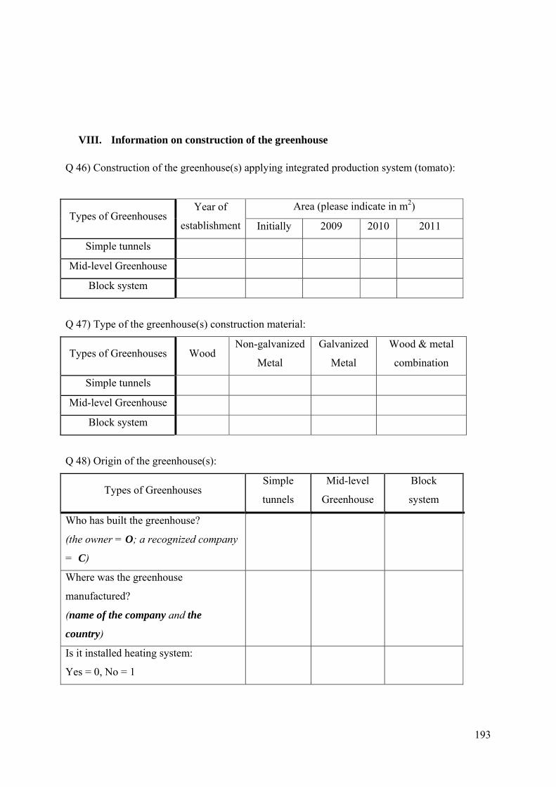
193

VIII. Information on construction of the greenhouse

Q 46) Construction of the greenhouse(s) applying integrated production system (tomato):

Types of Greenhouses Year of

establishment

Area (please indicate in m2)

Initially 2009 2010 2011

Simple tunnels

Mid-level Greenhouse

Block system

Q 47) Type of the greenhouse(s) construction material:

Types of Greenhouses Wood Non-galvanized

Metal

Galvanized

Metal

Wood & metal

combination

Simple tunnels

Mid-level Greenhouse

Block system

Q 48) Origin of the greenhouse(s):

Types of Greenhouses Simple

tunnels

Mid-level

Greenhouse

Block

system

Who has built the greenhouse?

(the owner = O; a recognized company

= C)

Where was the greenhouse

manufactured?

(name of the company and the

country)

Is it installed heating system:

Yes = 0, No = 1

194

Q 49) Present condition of the greenhouse(s):

Types of Greenhouses Simple

tunnels

Mid-level

Greenhouse

Block

system

What is the height of the

greenhouse(s)?

(indicate in meters)

Type of cover used:

(plastic = P + durability in years;glass

= G + durability in years)

What kind of ventilation system does

the greenhouse(s) have?

(front& back = F&B; lateral = L; roof

= R; lateral + roof = L&R.)

What kind of irrigation system is used

in the greenhouse(s)?

(drip irrigation = DI; sprinkler = S;

both = DI&S; none = N )

What is the source of the water supply?

(a well = W; a river = R - state name;

water pipes = P - state company; or

another source = state it)

What heating system is used?

(none = N; diesel = D; gas = G; wood

= W; coal = C; another fuel = state it)

During what period of the year are the

greenhouses used?

(from month X to month Y)

What vegetables do you cultivate in

195

GH?

(tomatoes = T; cucumbers = C;

peppers = P; lettuce = L; other = state

which).

Q 50) Waste Management:

What do you do with the old or damaged plastic?

I use it for other purposes [_______]

I burn it [_______]

I throw it away [_______]

I sell it to recycling companies [_______]

Other (please indicate): [_______]

Q 51) Future investment plan:

Do you have a plan to expand your agricultural activities applying IPM production system?

[0] [ ] Yes [1] [ ] No

If the answer is yes, what will be the source of the investment?

A bank loan [_______]

Own savings [_______]

Other sources (please indicate) __________ [_______]

Q 52) How much money did you spend on building the greenhouses you apply Integrated

Production System?

Building material Capacity Price in€ Total value€

Construction material

Covering

Heating system

Irrigating system

Ventilation system

Well

196

Q 53) What kind of mechanization do you have? Please indicate the type of mechanization, year

and money you spent buying it.

Type of mechanization Year Price in €

Total

Q 54) What are other equipment you use in farming activities? Please indicate the type of

equipment, year, and money you spent buying it.

Type of equipment Year Price in €

Pump for irrigation

Pump for spraying

Other (please indicate):

_____________________

_____________________

_____________________

_____________________

_____________________

_____________________

Total

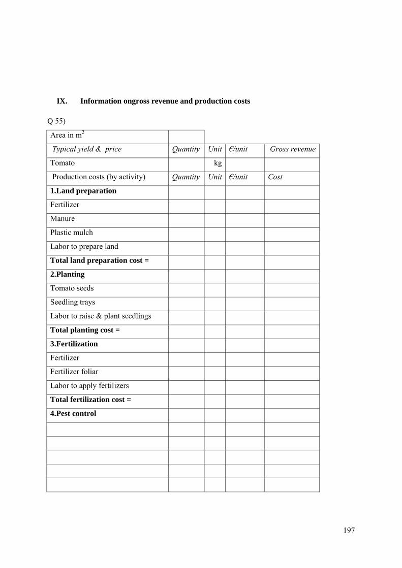
197

IX. Information ongross revenue and production costs

Q 55)

Area in m2

Typical yield & price Quantity Unit €/unit Gross revenue

Tomato kg

Production costs (by activity) Quantity Unit €/unit Cost

1.Land preparation

Fertilizer

Manure

Plastic mulch

Labor to prepare land

Total land preparation cost =

2.Planting

Tomato seeds

Seedling trays

Labor to raise & plant seedlings

Total planting cost =

3.Fertilization

Fertilizer

Fertilizer foliar

Labor to apply fertilizers

Total fertilization cost =

4.Pest control

198

Labor to apply pesticides

Total pest control cost =

5.Irrigation

Water

Labor to apply water

Total irrigation cost =

6.Warming

Fuel

Labor to apply warming

Total warming cost =

7.Harvesitng

Taking care, pruning, etc.

Labor to harvest

Boxes

Total harvesting cost =

8.Marketing

Labor to transport to market

Total marketing cost =

9.Mechanized operations

Fuel, oil & lube

Total machinery cost =

10.Operating overhead

Operating interest

Excise tax

Commissions

Management

Office overhead

Total operating overhead =

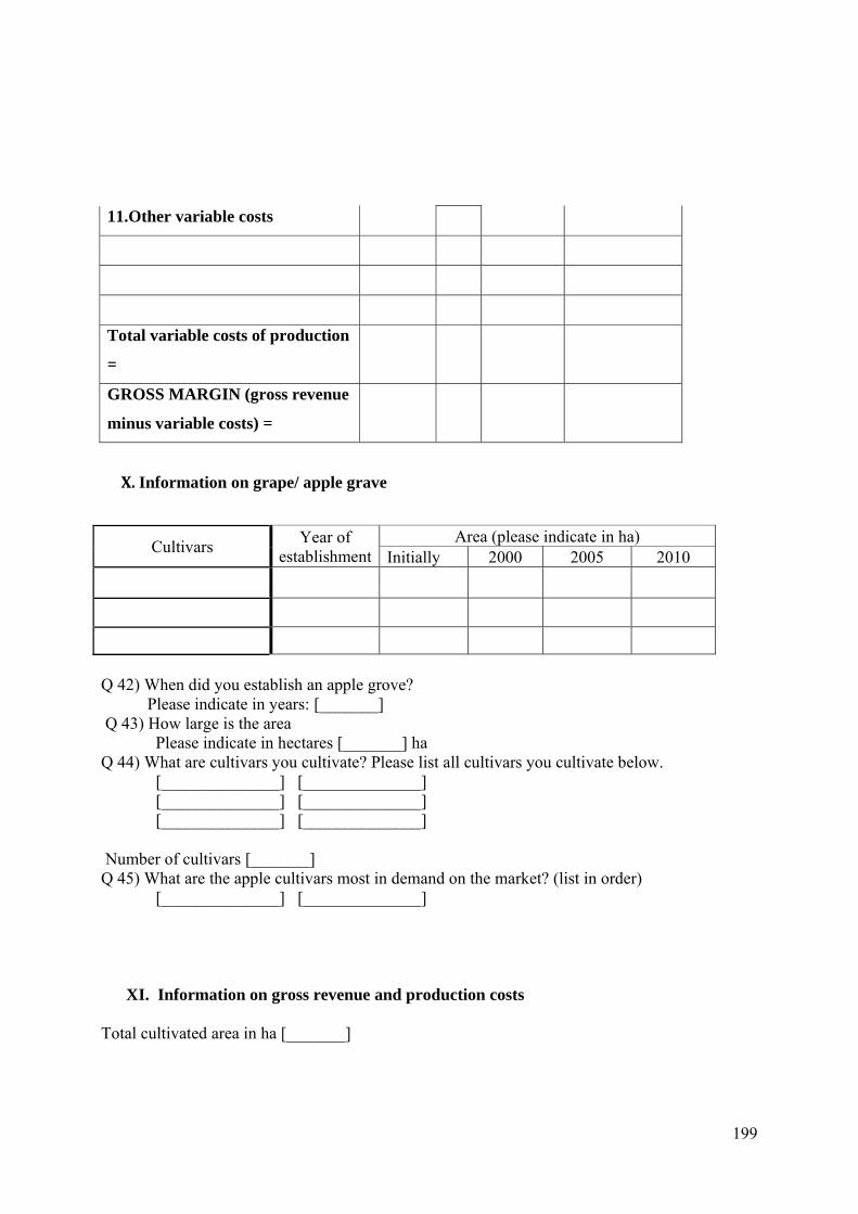
199

11.Other variable costs

Total variable costs of production

=

GROSS MARGIN (gross revenue

minus variable costs) =

X.Information on grape/ apple grave

Cultivars Year of

establishmentArea (please indicate in ha)

Initially 2000 2005 2010

Q 42) When did you establish an apple grove? Please indicate in years: [_______] Q 43) How large is the area Please indicate in hectares [_______] ha Q 44) What are cultivars you cultivate? Please list all cultivars you cultivate below. [______________] [______________] [______________] [______________] [______________] [______________] Number of cultivars [_______] Q 45) What are the apple cultivars most in demand on the market? (list in order) [______________] [______________] XI. Information on gross revenue and production costs Total cultivated area in ha [_______]

200

Q 46) Costs of producing apple: Production costs (by activity) Quantity Unit €/unit Cost Variable costs Pruning Training Fertilization Manure Fertilizer Foliar fertilizer Labor to apply fertilizers Total fertilization cost = Beehives Pest control Labor to apply pesticides Total pest control cost = Irrigation Water Electricity/Fuel Labor to apply water Total irrigation cost = Harvesting Picking labor Other labor (checkers, tractor drivers) Boxes Hauling apples Total harvesting cost = Marketing Labor to transport to market Transport costs Total marketing cost = Mechanized operations Fuel, oil & lube Maintenance and repairs

201

Fixed costs Interest Depreciation Taxes (land) Other expenses Cultivars Number

of trees Yield Price in euro

per kg Total Q 47) Future investment plan Do you have a plan to expand cultivated area with apple? [0] [ ] Yes [1] [ ] No If the answer is yes, what will be the source of the investment? A bank loan [_______] Own savings [_______] Other sources (please indicate) __________

[_______]

Q 48) What were the main diseases appeared last year: ____________________________ ____________________________ ____________________________ ____________________________ ____________________________

202

Q 49) What kind of mechanization do you have? Please indicate the type of mechanization, year and money you spent buying it. Type of mechanization Year Price in

euro2

Actual price in euro

Number of total hours used within a year

Number of total hours used in apple production

Total

Q 50) What are other equipment you use in farming activities? Please indicate the type of equipment, year, and money you spent buying it. Type of equipment Year Price in

€3

Actual price in market

Number of total hours used within a year

Number of total hours used in apple production

Pump for irrigation Pump for spraying Other (please indicate): _____________________ _____________________ _____________________ _____________________ _____________________ _____________________ Total

2 (whentheequipmentwasbought) 3 (whentheequipmentwasbought)

203

I. Information on fertilizer and pesticide application

56) Fertilizer application record

MAKE A RECORD OF EACH APPLICATION OF EACH FERTILIZER

App.

1

App.

2

App

3

App.

4

App.

5

Field or Site Location (give name or number of the field

treated)

Date (Day, Month Year):

Size of Area Treated (in m2):

Fertilizer Used (Brand Name) and total amount applied

____________________________

____________________________

____________________________

____________________________

____________________________

____________________________

Crop/Commodity or Site

Formulation

Additives

204

Method of Application

Stage of Crop Growth

Purpose of Application

Temperature

Time of Day

Wind

Cloud Cover

Effectiveness

Q57) Pesticide application record

MAKE A RECORD OF EACH APPLICATION OF EACH PESTICIDE

App.

1

App.

2

App

3

App.

4

App.

5

Field or Site Location (give name or number of the field

treated)

Date (Day, Month Year):

Size of Area Treated (in m2):

Pesticide Used (Brand Name) and total amount applied

InsecticideFungicideHerbicide

205

Crop/Commodity or Site

Formulation

Additives

Method of Application

Stage of Crop Growth

Purpose of Application

Stage of Development of Pest

Soil Conditions

Temperature

Time of Day

Wind

Cloud Cover

Effectiveness

206

Annex 3. Gross margins of tomato producers

A

INCOME Unit Quantity Price/Unit Value Quantity (ha)

Value (EUR/ha)

1.1 Total tomato yield Kg/ha 137,500 0.26 35,750.00 85937.50 22343.75

Total income 35,750.00 22343.75

2 VARIABLE COSTS

2.1 Inputs

Seeds-Sapling Sapling 33000 0.13 4,158.00 20625.00 2681.25

Artificial fertilizer (NPK) kg/ha 925 0.60 555.00 578.13 346.88

Manure kg/ha 55500 0.03 1,480.00 34687.50 1040.63

Crystaline Fertilizer kg/ha 990 0.68 668.92 618.75 420.75

Foliar feeding l/ha 0.00 0.00 0.00 0.00 0.00

Total pesticides kg/l/ha 0.00 0.00 119.00 0.00 74.38

Plastic mulch m2 0.00 0.00 0.00 0.00 0.00

Packing (boxes) piece 27500 0.28 7,700.00 17187.50 4812.50

Irrigation 0.00 0.00 0.00 0.00 150.00

Total inputs 14,680.92 9526.38

2.2 Mechanized operations

Plugging l/diesel 60 1.2 72.00 37.50 45.00

Harrowing l/diesel 60 1.2 72.00 37.50 45.00

Planting l/diesel 10 1.20 12.00 6.25 7.50

Fertilization l/diesel 0.00 0.00 0.00 0.00 0.00

Spraying l/diesel 0.00 0.00 0.00 0.00 0.00

Diesel fuel for irrigation l/ha 345 1.20 414.00 215.63 258.75

Transport to market Lump sum 375 1.20 450.00 234.38 281.25

Maintenance Lump sum 25.00

Total working machinery costs 1,020.00 662.50

B Total variable costs 15,700.92 10188.88

3 CONTRIBUTION MARGIN (A-B) 20,049.08 12154.88

4 FAMILY LABOUR FORCE

Labor to prepare land p/d 2.0 15.00 30.00 1.25 18.75

Planting p/d 70.0 15.00 1,050.00 43.75 656.25

Fertilization p/d 10.0 15.00 150.00 6.25 93.75

Spraying p/d 24.0 15.00 360.00 15.00 225.00

Seedlings connection p/d 70.0 15.00 1,050.00 43.75 656.25

Removal of buds p/d 120 15.00 1,800.00 75.00 1125.00

207

Harvesting p/d 450.0 15.00 6,750.00 281.25 4218.75

Transport to market p/d 15.0 15.00 225.00 9.38 140.63

Total work 761.00 11,415.00 475.63 7134.38

5 GROSS MARGIN BEFORE DEPRECIATION

8,634.08 5020.50

Depreciation Lump sum

1,241.32 1241.32

6 NET MARGIN WHEN 100% OF WORKS CARRIED OUT BY FAMILY MEMBERS

20,049.08 10913.55

Works carried out by family members 11,415.00 7134.38

NET REVENUE 8,634.08 3779.18

208

Annex 4. Gross margins of grape producers

Unit Quantity Price

per unit Value in

EUR % Quantity

(ha) Valu in

EUR (ha)

REVENUE

Grapes kg/ha 27,520 0.25 6742.4

11,965.22

2,931.48

Subsidy EUR/ha 0 0

Total income 6742.4

100% 0

2,931.48

VARIABLE COST 0 0

Inputs 0 0

Strings kg/ha 4.6 3.00

13.80 2 6

NPK kg/ha 900 0.46

410.0

391.30

178.26 NAG kg/ha 0 0.00

0.0 0 0

Leaf fertilizer kg/ha 0 0.00

0.0 0 0

Pesticides kg/ha 11 23.09

254.0

4.78

110.43

Other consumables Lump sum

0.0 0

-

Total inputs 677.80 10% 0

294.70

Machinery services 0 0

Spring plowing (2 times) l/diessel

268 1.20 321.60

116.52

139.83

Autum plowing (2 times) l/diessel

268 1.20 321.60

116.52

139.83

Cultivation (2 times) l/diessel 268 1.20 321.60

116.52

139.83

Fertilization NPK l/diessel 20 1.20 24.00

8.70

10.43

Additional fertilization NAG l/diessel 0.00 0.00

0 0

Spraying (3 times) l/diessel 75 1.20 90.00

32.61

39.13

Other works l/diessel 0 0.00 0.00 0 0

Total cost of machinery services 1,078.80

16% 0

469.04

Marketing costs 0.00 0 0.00 0 0

Transport Operations 37.5 4.00 150.00

16.30 65.2173913

Total cost of marketing 150.00 2% 0

65.22

Total variable costs 1906.60 28% 0

828.96

CONTRIBUTION MARGIN (A-B) 4835.80 0

2,102.52

209

Labour 0 0

Pruning p/d

29 0.00 0.00

12.61

-

Cleaning vines p/d 0 0.00 0.00

0 0

Maintenance p/d 0 0.00 0.00

0 0

Binding vines p/d

10 0.00 0.00

4.35

-

Digging, cleaning soil p/d 0 0.00 0.00

0 0

Removing weeds (2 times) p/d

16 0.00 0.00

6.96

-

Binding branches p/d 0 0.00 0.00

0 0

Spraying (3 times) p/d

3 15.00 45.00

1.30

19.57

Harvesting p/d

20 0.00 0.00

8.70

-

Total labour costs 78.00 45.00 0.67%

33.91

19.57

GROSS MARGIN BEFORE DEPRECIATION 4790.80 0

2,082.96

Depreciation Lump sum 300.00 4.45% 0

130.43

NET MARGIN WHEN 100% OF WORKS CARRIED OUT BY FAMILY MEMBERS 4490.80 66.61% 0

1,952.52

210

Annex 5: Gross margins of apple producers

Unit Quantity/ ha Unit price Euro Total cost Euro/ha

Apples kg/ha 32000 0.36 11520

Total income 11520

VARIABLE COST

Inputs

Manure Mt/ha 60 5 300

Fertilizer kg/ha 825 0.7 577.5

PPP kg/ha 14 60 840

Total inputs 1767.5

Works

Cultivation between rows service/day 3 30 90

Spraying (6 times) service/day 6 30 180

Other works Lump sum 100

Total works 370

Marketing costs

Boxes Pieces 4000 0 0

Transport Operations 14 50 700

Total marketing 700

Total variable costs 2837.5

GROSS MARGIN 8682.5

Labour

Pruning Price per tree 1600 1 1600

Manuring p/d 8 15 120

Fertilizing p/d 2 15 30

Irrigating p/d 2 15 30

Spraying p/d 14 15 210

Fruit thinning p/d 8 15 120

Harvesting p/d 80 15 1200

Other labor p/d 2 15 30

Total labour 128.00 3,340.00

300.00

NET MARGIN 5342.5

211

Ich erkläre: 'Ich habe die vorgelegte Dissertation selbständig und ohne unerlaubte fremde Hilfe

und nur mit den Hilfen angefertigt, die ich in der Dissertation angegeben habe. Alle Textstellen,

die wörtlich oder sinngemäß aus veröffentlichten Schriften entnommen sind, und alle Angaben,

die auf mündlichen Auskünften beruhen, sind als solche kenntlich gemacht. Bei den von mir

durchgeführten und in der Dissertation erwähnten Untersuchungen habe ich die Grundsätze guter

wissenschaftlicher Praxis, wie sie in der Satzung der Justus-Liebig-Universität Gießen zur

Sicherung guter wissenschaftlicher Praxis niedergelegt sind, eingehalten.'

Gießen, den ____________________

efficiency analysis of alternative production systems in...

Documents