TGU-ECON Discussion Paper Series

#2020-2

Efficiency and Group Size in the Voluntary Provision of Public Goods with Threshold Preference

Yoshito Funashima

Faculty of Economics, Tohoku Gakuin University

February 2020

Efficiency and group size in the voluntary provision of

public goods with threshold preference∗

Yoshito Funashima†

Faculty of Economics, Tohoku Gakuin University

February 5, 2020

Abstract

What is the optimal group size in the voluntary provision of public goods in a

purely altruistic economy? The popular consensus on this fundamental question is

that the free-rider problem worsens as group size increases. This study provides a

counterexample to the consensus, featuring threshold preferences that are plausible

for certain typical public goods. Under these threshold preferences, marginal utility

hardly diminishes below a threshold level, but declines significantly around the

threshold, becoming almost zero over the threshold. We show that the threshold

preferences significantly reduce inefficiency. We also show that if the marginal cost

increases, the threshold preferences are contrary to the consensus and lead to a

partly positive relationship between efficiency and group size, thereby detecting the

local efficient group size. Moreover, the local efficient group size is proportional to

the slope of marginal cost as well as the threshold of marginal utility.

Keywords: Threshold preferences, Voluntary provision of public goods, Group size

JEL classification: H41, D61

∗Financial support for this research from a Grant-in-Aid for Scientic Research by the Japan Societyfor the Promotion of Science (No. 17K03770) is gratefully acknowledged.

†1-3-1 Tsuchitoi, Aoba-ku, Sendai, Miyagi 980-8511, Japan; E-mail: funashima@mail.tohoku-gakuin.ac.jp

1

1 Introduction

What effect the group size of a voluntary economy has on the degree of efficiency in the

private provision of public goods has been one of the fundamental questions in public eco-

nomics since the pioneering work of Olson (1965). To date, many researchers have studied

the issue and theoretical studies have reached a broad consensus that there is a mono-

tonically decreasing relationship between efficiency and group size in a purely altruistic

economy with noncooperative contributors, as shown by Andreoni (1988), among others.1

The theoretical consensus is robust regardless of the type of standard preferences.2

Although we often take such consensus for granted, in this study, we show that, in

particular cases, there is more to this issue than previously thought. In the early theo-

retical works, the possible preference features of public goods have not been sufficiently

addressed.3 Recognizing that there would be no appropriate preferences for all types

of public goods, it is all the more important to investigate how (in)efficient resource al-

locations can arise from every conceivable angle. Specifically, it cannot be ruled out a

priori that the diminishing degree of marginal utility depends to a greater extent on the

consumption level than usual. As part of the possible preferences, the present analysis

considers the case of individuals who have a threshold preference for public goods con-

sumption. Under this threshold, marginal utility hardly diminishes below a minimum

threshold, but declines significantly around the threshold, becoming close to zero over the

threshold; that is, unlike the standard case, utility increases in an approximately linear

fashion below the threshold and hardly increases over the threshold, as shown in Figure

1. We refer to this as individuals’ threshold preference (of public goods).

[Insert Figure 1 around here]

The threshold preference is in fact considered plausible in some cases of well-recognized

public goods such as charitable volunteer activities and clean environments. For example,

one could imagine a charity for natural-disaster victims as a social contribution issue. In

this case, the marginal utility of supportive activities could potentially decrease very little

1In this study, unless otherwise noted, we use “altruism” to mean the pure altruism in which individualshave a preference depending only on the total supply of the public goods. While beyond the scope of thisstudy, a branch of the literature considers impure altruism (warm-glow giving) in which individuals havea preference depending on their own contributions, including Harbaugh (1998) and Diamond (2006). SeeAndreoni (1990) for the details of an impure altruism case. In addition, while also beyond the scopeof this study, some research highlights the role of the cooperative behavior of contributors; see Wilson(1992), Pecorino (1999), Fehr and Gachter (2000), and Keser and Winden (2000), among others.

2See, e.g., Mueller (1989) for Cobb–Douglas preferences and Cornes and Sandler (1985) for quasi-linearpreferences. Isaac and Walker (1988) provide experimental support for the theoretical consensus.

3One important exception is Hayashi and Ohta (2007), who consider the satiation at some consumptionlevels of public goods, as detailed below.

2

at insufficient levels of total contributions, because the victims still tolerate the inconve-

niences of an unsettled lifestyle. Rather than assuming an immediately diminishing rate

of the marginal utility, it is more likely that the marginal utility substantially decreases

only after total contributions are sufficient to aid the victims. Once their standard of

living is sufficiently restored, the marginal utility could become virtually zero.

As another example, consider garbage-strewn beaches and a local beach clean-up effort

as an environmental issue. Irrespective of how much some people clear up the garbage,

the marginal utility of additional clean-up would remain high, as long as the remaining

garbage stands out, thereby spoiling an intrinsically beautiful landscape. Only after

beaches are restored to a satisfactory level of cleanliness, would the marginal utility finally

begin to noticeably decrease. Eventually, little marginal utility is derived from removing

the remaining very small and inconspicuous garbage.

In contrast to the preceding theoretical consensus, our analysis reveals that public

goods provision in the Nash equilibrium can lead to approximately efficient outcomes.

To this end, we consider a very simple and standard model in the literature assuming

an altruistic economy, except the utility function with the following three features: (a)

marginal utility is relatively slowly-diminishing when public goods are below the threshold,

(b) it is relatively sharply-diminishing only when public goods provision is in the vicinity

of a threshold value, and (c) it is almost zero when it exceeds the threshold. We emphasize

that these three features are involved with relative changes in the marginal utility and

retain the standard assumptions; that is, positive marginal utility and law of diminishing

marginal utility. Thus, our analysis is in line with the underlying framework in the

altruism literature, but it nevertheless reaches a conclusion that voluntary provision of

public goods can attain approximately efficient resource allocations.

In addition, we find that if the marginal cost of contributions by individuals is in-

creasing, the threshold preferences are contrary to the broad consensus that an increase

in group size inevitably makes efficiency worse. Although much of the previous litera-

ture assumes constant marginal cost, increasing marginal cost seems rather natural in

the provision of some public goods. For example, in the case in which the provision of

public goods involves some sort of physical tasks, contributors are gradually fatigued as

their contributions increase and they eventually become exhausted. The aforementioned

examples, charitable volunteer activities and environmental cleaning, apply to this case.4

On the basis of this natural assumption, we demonstrate that the threshold preferences

lead to a partly positive relationship between efficiency and group size, detecting the local

efficient group size. Within the confines of simple noncooperative behavior of contributors

in a purely altruistic economy, the present study is first to uncover the existence of the

4Other examples of the increasing marginal cost can be found in Hayashi and Ohta (2007).

3

local efficient group size.

This study is at the crossroads of two lines of research. One is the work raising the

issue of efficiency–group size nexus in the voluntary provision of public goods in a purely

altruistic economy, with certain representative studies already mentioned above. Among

others, Hayashi and Ohta (2007) deserves special mention as an important precursor to

this study. The authors took a step in this direction by positing two assumptions: in-

creasing marginal cost of voluntary provision and the existence of a finite satiety point

in utility. As a result, they claim that inefficiency is alleviated as group size increases,

and optimality is achieved when group size approaches infinity. While their work overlaps

with ours, there are notable differences in both assumptions and findings. Specifically,

we assume threshold preferences instead of a finite satiety point in utility and find sub-

stantial improvements in efficiency when group size is not infinite. The characteristics of

threshold preferences are similar to the assumption of satiation in that the threshold level

of provision could be interpreted as roughly corresponding to the satiation level; how-

ever, there are crucial differences between the two—in threshold preferences, marginal

utility is slowly-diminishing below the threshold level and sharply-diminishing around the

threshold level. In addition to these differences in preferences, we relax the assumption

of the increasing marginal cost, in which the marginal cost is required to approach zero

as contributions by individuals approach zero.

The second line of research is characterization of types of public goods (e.g., pure

and impure public goods). Traditionally, there are various types, such as congestible

goods and local public goods. In this line of research, this study is most closely related

to the recently growing body of literature on the so-called threshold public goods (e.g.,

Cadsby and Maynes, 1999; Spencer et al., 2009; Corazzini et al., 2015; Li et al., 2016;

Brekke et al., 2017). While much of the literature exploits experimental approaches to

investigate a public goods game, threshold public goods are characterized as those that

are consumable only when total contributions surpass a minimum threshold (provision

point). Thus, threshold public goods and the present threshold preferences are analogous

in that total contributions have meaningful threshold values; however, they critically differ

from each other in that marginal utility is positive only after total contributions exceed

a critical level in threshold public goods whereas it is sizable only when below a critical

level in threshold preferences.

The rest of this paper is organized as follows. In section 2, we formally define threshold

preferences and present our model. In section 3, we analytically examine the relationship

between efficiency and group size. In section 4, we provide further results using numerical

analysis. Concluding remarks are presented in section 5.

4

2 Basic theory

2.1 The model

Consider an economy in which n identical individuals exist, with n ∈ (1,∞). Let x and

G denote a private good (numeraire) and a public good, respectively. The individuals are

considered to have preferences that are represented as a quasilinear utility function

U = U(x,G) = x+ f(G), (1)

where f(G) satisfies the standard assumptions, and is strictly increasing and concave,

f ′ > 0 and f ′′ < 0. The marginal rate of substitution is given by

π(G) =∂U/∂G

∂U/∂x= f ′(G). (2)

As explained in our introduction, we assume threshold preferences in which the marginal

utility, ∂U/∂G = f ′(G), is rapidly diminishing around a threshold level of public goods

γ. Staying coordinated with the above standard features of utility function, threshold

preferences are defined in the following way.

Definition 1. The utility function U(x,G) is called a threshold utility function if the

marginal utility, ∂U/∂G = f ′(G) > 0, is a twice continuously differentiable function with

f ′′(G) < 0 for all G ∈ [0,∞), and if it satisfies the following properties:

(i) limG→∞ f ′(G) = 0, and limG→∞ f ′′(G) = 0.

(ii) f ′(G) has a unique inflection point (γ, f ′(γ)); that is, f ′′′(G) = 0 if and only if G = γ.

(iii) f ′(G) is a strictly concave (convex) function when G < γ (G > γ); that is, f ′′′(G) ≷ 0

if and only if G ≷ γ.

(iv) An arbitrary small neighborhood of γ, (γ − γl, γ + γh) exists, such that

0 ≲∣∣∣f ′′(G)

∣∣G/∈(γ−γl, γ+γh)

∣∣∣ ≪ 1 ≪∣∣∣f ′′(G)

∣∣G=γ

∣∣∣, (3)

where γl, γh > 0, and f ′′(G)∣∣G=γ

is a global minimum.

A public good is supplied by individuals’ voluntary contributions, and the total con-

tributions G are the sum of all individuals’ voluntary contribution g (i.e., G =∑

g). An

individual’s endowment w is divided into two parts: private consumption x and the cost

of producing their contribution to a public good c(g). Hence, each individual faces the

budget constraint

w = x+ c(g). (4)

5

As the property of cost function c(g), we consider the two cases of the marginal cost c′(g).

The first case is a standard assumption in the literature, that is, the marginal cost is

positive and constant (i.e., c′(g) = θ > 0). In the second case, as in Hayashi and Ohta

(2007), the marginal cost is assumed to be increasing (i.e., c′′(g) > 0). In what follows,

to examine the relationship between group size and efficiency, we assume the following

conditions for each case.

Assumption 1. If c′(g) is constant θ, then 0 < θ < f ′(0).

Assumption 2. If c′(g) is increasing and c′′(g) > 0, then 0 ≤ c′(0) < f ′(0).

While both assumptions are required to guarantee that solutions are interior, we make

some remarks on Assumption 2, which is related to Hayashi and Ohta (2007). To present a

counterexample to the inverse relationship between group size and efficiency, Hayashi and

Ohta (2007) impose a restriction on increasing marginal costs, such that they approach

zero as g → 0 (i.e., c′(0) = 0). Note that Assumption 2 encompasses this restriction and

allows for the positive values (i.e., c′(0) > 0).

2.2 Nash equilibrium and efficient resource allocation

The present problem with Nash behavior of an individual is to maximize (1) subject to (4)

by choosing x and g, given contributions by others. Noting that our model is an identical

economy, the following equation is satisfied in Nash equilibrium

f ′ (G)= c′ (g) , (5)

where G = ng, and upper bars represent the equilibrium values. In preparation for the

following analysis, it is useful to consider the group size elasticity. Totally differentiating

(5) with respect to G and n yields the group size elasticity of equilibrium provision:

dG

dn

n

G=

c′′ (g) /n

c′′ (g) /n− f ′′(G) . (6)

On the other hand, solving the problem to maximize (1) subject to (4) by choosing x

and G, we obtain the Samuelson condition:

f ′ (G∗) =c′ (g∗)

n, (7)

where G∗ = ng∗, and asterisks represent optimal values. As before, totally differentiating

(7) with respect to G∗ and n yields the group size elasticity of optimal provision:

dG∗

dn

n

G∗ =c′′ (g∗) /n+ c′ (g∗) /G∗

c′′ (g∗) /n− nf ′′ (G∗). (8)

6

3 Efficiency and group size

We now examine the discrepancies between Nash and optimal provisions under the thresh-

old preferences. We begin by examining the case in which marginal costs are constant.

3.1 Constant marginal costs

In the case of constant marginal costs, the right-hand side (RHS) of (5) is θ and that of (7)

is θ/n. Thus, G∗ increases as n increases, whereas G does not depend on n; accordingly,

an inverse relationship exists between group size and efficiency. This inverse relationship

can also be confirmed in terms of group size elasticity. Since c′′ = 0, the Nash group

size elasticity in (6) becomes zero. In contrast, the optimal group size elasticity in (8) is

−θ/ [nG∗f ′′ (G∗)], while it takes positive values and converges zero as n → ∞.

[Insert Figure 2 around here]

Thus, G∗−G inevitably increases as n increases due to the law of diminishing marginal

utility (f ′′(G) < 0); however, given the group size n, the threshold preferences could

alleviate the inefficiency of the private provision of a public good. To confirm our intuition,

we depict the representative shape of (5) and (7) as Figure 2, in which Panels A and B

respectively show the cases of standard and threshold preferences. Under the standard

preferences, marginal utility f ′(G) immediately decreases, and the left-hand side (LHS)

of (5) and (7) has a markedly negative slope even when G is small. By contrast, in the

case of the threshold preferences, the slope of marginal utility is flatter for small values

of G and steeper around G = γ than in the case of the standard preferences. As a result,

given the group size n, the Nash equilibrium provision G increases and approaches the

optimal provision G∗. In particular, when the curvature of marginal utility approaches

infinity, both G and G∗ converge to the threshold level γ, as shown by the dashed line in

Panel B of Figure 2.

In summary, the following proposition is obtained.

Proposition 1. Assume that marginal costs are constant and Assumption 1 holds. Then,

while G∗ − G increases as n increases, it decreases as the curvature of the threshold

preferences becomes large.

3.2 Increasing marginal costs

Turning to the case of increasing marginal costs, the slope of the RHS of (5) can be

represented as c′′(G/n)/n and decreases as n increases. It follows that G is strictly

7

increasing in n, unlike the case of constant marginal cost. The slope of the RHS of (7) is

c′′(G/n)/n2 and smaller than that of (5) for all G.

[Insert Figures 3 and 4 around here]

Even when assuming increasing marginal cost, the introduction of the threshold pref-

erences could make the voluntary provision less suboptimal. As before, Figure 3 shows

the representative shape and illustrates how the introduction of the threshold preferences

alleviates suboptimality. Panels A and B depict the standard and threshold preferences,

respectively. The figure exemplifies that if we assume the threshold preferences, then G

increases and G∗ decreases. It should be noted that in contrast to the case of constant

marginal costs, this exemplification is not universally applicable for any n. Specifically,

consider a case in which n is small and the slopes of the RHS of (5) and (7) are steep, as

shown in Figure 4. In the figure, a red line represents the LHS in threshold preferences.

In this situation, G∗ −G increases as the curvature of the threshold preferences becomes

large. The main results are summarized in the following proposition.

Proposition 2. Suppose that marginal costs are increasing and Assumption 2 holds.

Then, G∗ −G decreases as the curvature of the threshold preferences becomes large, pro-

vided that n is not small.

We next investigate how the inefficiency G∗ − G relates to the group size n. First,

noting that limn→1G = limn→1G∗, we denote the limits as Ginf . It is obvious that if we

consider a situation such that Ginf ≥ γ, then G∗ −G is monotonically increasing with n.

To exclude the monotonicity case, we assume the following condition:

Assumption 3. If c′(g) is increasing and c′′(g) > 0, then Ginf < γ.

Assumption 3 implies that the threshold level γ is not an extremely small amount.

[Insert Figure 5 around here]

Importantly, whileG∗ is larger thanG for any n, G∗−G is not monotonically increasing

with n, provided that Assumption 3 is satisfied. The reason behind the non-monotonicity

is straightforward, and we can understand this by considering the potential three stages

of group size. In the first stage, where group size is small (G ≪ γ) and f ′′ ≃ 0 as shown

in Panel A of Figure 5, we can respectively reformulate the group size elasticity in (6)

and (8) as

dG

dn

n

G≃ 1, (9)

dG∗

dn

n

G∗ ≃ 1 +nc′ (g∗)

G∗c′′ (g∗). (10)

8

It evidently follows that the optimal group size elasticity is larger than the Nash group

size elasticity, and G∗ −G is increasing with n when n is small.

In the second stage, where group size n is large to some extent and G∗ reaches the

values around the threshold level γ as shown in Panel B of Figure 5, the optimal group

size elasticity in (8) becomes approximately zero because f ′′(G∗) takes large negative

values. On the other hand, G is smaller than γ and the Nash group size elasticity in (6) is

positive. In this case, the Nash group size elasticity is larger than the optimal group size

elasticity, and G∗ − G is decreasing with n. In a limiting case, as shown by the dashed

line in Panel B of Figure 5, when the curvature of marginal utility approaches infinity,

the Nash equilibrium provision and the efficient provision converges.

In the last stage, as shown in Panel C of Figure 5, when group size n is sufficiently

large so that c′′ (g∗) /n ≃ 0, and f ′′ (G∗) ≲ 0 so that nf ′′ (G∗) takes finite values,

dG

dn

n

G≃ 0, (11)

dG∗

dn

n

G∗ ≃ − c′ (g∗)

G∗nf ′′ (G∗). (12)

This suggests that when group size n is sufficiently large, G∗ −G is increasing with n.

The second and third stages indicate that a U-shaped relationship exists between

G∗ − G and n, meaning the existence of local efficient group size n∗. Thus, we establish

the following proposition:

Proposition 3. Suppose that marginal costs are increasing and Assumptions 2 and 3

hold. Then, a unique n∗ that locally minimizes G∗ −G around G = γ exists.

This result is striking and has some important implications. A monotonically inverse

relationship between efficiency and group size in the private provision of public goods is

a widely accepted result; that is, a large group size aggravates the free-rider problem.

However, Proposition 3 indicates that even if group size becomes large, the efficiency

could be better. This implies, for example, that there is suboptimal population size n∗ of

nations or local municipalities, when some national or local public goods are voluntarily

provided.

[Insert Figures 6 and 7 around here]

It is intuitive that n∗ depends on γ. Figure 6 illustrates the effect of an increase in

γ. In this case, f ′(G) locus shifts right by the amount of the increase in γ from γ1 to γ2.

When γ = γ1, G∗ −G is G∗

1 −G1 and small. When γ = γ2, G∗ −G becomes G∗

2 −G2 and

larger; in this case, G∗ − G could substantially decrease by increasing n. This suggests

9

that n∗ becomes larger as γ increases. Moreover, n∗ depends on slopes of marginal costs,

c′′(g). Figure 7 exemplifies the case of increases in the slopes of marginal costs. Due to

the increases, both G∗ and G decrease, and there is room to decrease G∗−G by increasing

n. In other words, n∗ becomes larger as the slopes of marginal costs increase. Thus, from

Proposition 3, the following corollaries are immediately apparent.

Corollary 1. Suppose that marginal costs are increasing and Assumptions 2 and 3 hold.

Then, n∗ is proportional to γ.

Corollary 2. Suppose that marginal costs are increasing and Assumptions 2 and 3 hold.

Then, n∗ is proportional to c′′(g).

4 Quantitative analysis

The previous section analytically shows that threshold preferences could allow the allevi-

ation of inefficiency in the voluntary provision of public goods. In particular, if we assume

threshold preferences and increasing marginal cost, the general consensus undergoes mod-

ification. That is, the monotonical increasing relationship between inefficiency and group

size no longer holds.

In this section, we undertake several numerical analyses of the model, focusing on the

case of increasing marginal costs. Our purpose here is to illustrate the qualitative effects

of threshold preferences on inefficiency and to present further results that are analytically

ambiguous. For example, although the analysis thus far has explained the existence of

local efficient group size n∗, we still lack an understanding of the extent to which the local

efficient level deviates from the global efficient level. First, we consider the specification

of threshold preferences.

4.1 Parameterization

Up to this point, f(G) is not a specific function. To study this numerically, we now specify

threshold preferences. Note that, as shown below, the marginal utility of the following

specified utility function has the form whose graphs are seen to be mirror images of the

graphs of the logistic function with reference to the vertical axis. For this reason, we call

this an axisymmetric-logistic utility function, which has the following form.

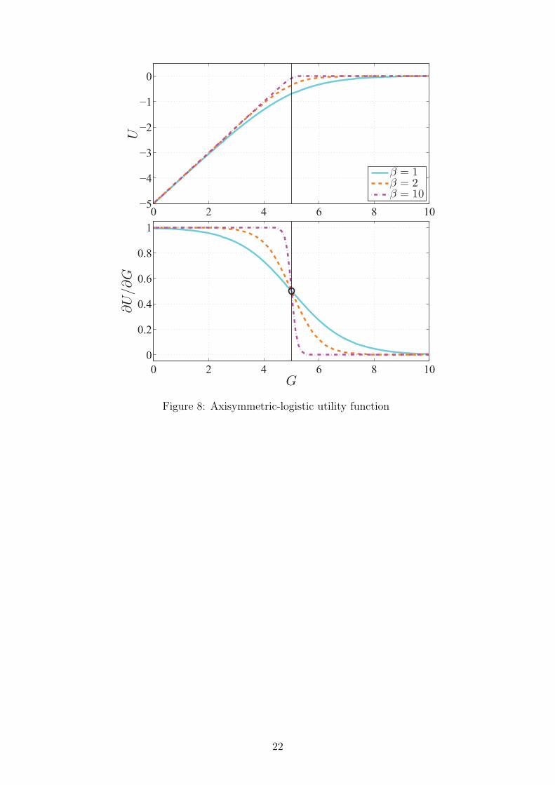
Definition 2. An axisymmetric-logistic utility function is defined as

U(x,G) = x− α

βln (1 + exp [−β(G− γ)]), (13)

with α, β, γ > 0.

10

Lemma 1. Consider the axisymmetric-logistic utility function. Then, it holds that

(i) the marginal utility, ∂U/∂G, is a twice continuously differentiable function and satisfies

the law of diminishing marginal utility.

(ii) The marginal utility has a unique inflection point (γ, α/2).

(iii) If G < γ (G > γ), the marginal utility is a strictly concave (convex) function.

Proof. The law of diminishing marginal utility can be straightforwardly confirmed, such

that

∂U

∂G=

α exp [−β(G− γ)]

1 + exp [−β(G− γ)]> 0, (14)

∂2U

∂G2= − αβ exp [−β(G− γ)]

(1 + exp [−β(G− γ)])2< 0. (15)

Moreover, since we have

∂3U

∂G3=

αβ2 exp [−β(G− γ)] (1− exp [−β(G− γ)])

(1 + exp [−β(G− γ)])3⪌ 0 ⇔ G ⪌ γ, (16)

it is obvious that a unique inflection point of ∂U/∂G is (γ, α/2).

[Insert Figure 8 around here]

Lemma 1 means that this felicity function has the properties stated in Definition 1

of the threshold preferences. β and γ are key parameters characterizing the threshold

preferences. β determines the curvature of the marginal utility, and γ represents the

threshold levels. To confirm these, Figure 8 plots (13) and (14) when α = 1 and γ = 5

together with some values of β. When β = 1, the curvature of the utility function appears

to be relatively mild, the marginal utility declines across the board values of G. If we

examine the case of β = 2, the marginal utility declines at a narrower range centering

around G = γ = 5. When β = 10, the utility function is almost linear except the vicinity

of G = γ = 5, and accordingly, the marginal utility exhibits a sharp decline around the

threshold level. Thus, we have the next lemma.

Lemma 2. Consider the axisymmetric-logistic utility function. Then, when β is large,

this function is regarded as a form of threshold utility function.

To present quantitative analysis, specification of c(g) is also required. We then specify

the cost for the voluntary contribution to be quadratic

c(g) =ϕ

2g2 + ηg. (17)

11

From (5) and (7), the voluntary and optimal provision are respectively obtained by

solving the following equations

α exp[−β(G− γ)

]1 + exp

[−β(G− γ)

] = ϕg + η, (18)

α exp [−β(G∗ − γ)]

1 + exp [−β(G∗ − γ)]=

ϕg∗ + η

n. (19)

Since these cannot be solved analytically, we present the results on numerical solution

below.

There are five parameters characterizing the equilibria. From now on, unless otherwise

noted, we set α = 1, β = 1, and γ = 100 for the threshold preferences; similarly, ϕ = 1

and η = 0 for the cost function.

4.2 Effects of threshold preferences

Our first step is to provide an illustration of the basic result that the suboptimality is

improved when individuals have threshold preferences. Figure 9 shows the relationship

between group size n and inefficiency G∗ − G for various parameters of β. Note that

the figure is a double logarithmic plot, and the minimum of n is set to 2. Consistent

with Proposition 2, G∗ −G shrinks considerably when β is large, on the whole. When n

is small and less than approximately 10, G∗ − G rises. However, when β is large, such

rises appear much less pronounced. Furthermore, consistent with Proposition 3, when

β = 10−1, 100, and 101, a unique n∗ (local efficient group size) exists between 102 and

103. More importantly, in addition to these illustrations of Propositions 2 and 3, we find

that when β = 101, n∗ is not local minimum but a global minimum.

[Insert Figure 9 around here]

According to Corollary 1, higher threshold levels cause local efficient group size to

also be higher. Figure 10 illustrates this point by plotting the relationship between n and

G∗ − G for various γ. By definition, the degree of n∗ becomes higher as γ gets higher.

A striking pattern that emerges from the figure is that G∗ −G undergoes a much larger

change for higher γ; consequently, in contrast to the widespread consensus, a large group

size could substantially improve the efficiency of the private provision of public goods.

[Insert Figure 10 around here]

Similarly, according to Corollary 2, steeper slopes of marginal cost cause local efficient

group size to be also higher. In fact, Figure 11 shows that the degree of n∗ becomes higher

12

as ϕ increases, illustrating the result in Corollary 2. Compared with changes in γ (Figure

10), maximum values of G∗ −G are less influenced by changes in ϕ.

[Insert Figure 11 around here]

Finally, Figure 12 explores their relationships for various η. As expected, we notice

the qualitatively similar results to the case of ϕ, but the effects of η appear quantitatively

negligible. In comparison to Hayashi and Ohta (2007), what is more noteworthy is that

the outcomes are less sensitive to c′(0) (i.e., η in the present case). In Hayashi and Ohta’s

(2007) framework, the assumption that c′(0) = 0 is indispensable for achieving a notable

conclusion that the inefficiency converges zero as the group size approaches infinity. In

contrast, our results are robust to the situation in which c′(0) > 0.

[Insert Figure 12 around here]

Overall, the numerical results consistently exhibit that if individuals have threshold

preferences, the increasing relationship between group size and inefficiency is different

depending on group size; comparing the increasing phases, aggravation of efficiency is

more severe when group size is small than large. This offers a new insight that the

free-rider problem becomes less serious when group size is large rather than small.

5 Conclusion

Since Samuelson’s (1954) influential article, most undergraduate public economics text-

books state that public goods are underprovided in static games with voluntary contri-

butions and inefficiency arises in a general context. Moreover, there is now a general

consensus in the existing literature that the relationship between inefficiency and group

size is monotonically increasing. Although there is no doubt of the validity of such consen-

sus in general, this study has shed new light on this fundamental issue in particular cases.

In other words, there are plausible cases in which the inefficiency can be substantially

lessened and the monotonical increasing relationship is broken. To present the results, we

analyzed standard models except for a newly proposed preference of individuals, called

threshold preference. Although the proposed utility function seems plausible in some

types of public goods and satisfies standard assumptions such as the law of diminishing

marginal utility, it nevertheless alleviates inefficiency. Furthermore, if we additionally as-

sume increasing marginal cost, which also seems plausible in some cases, a local efficient

group size is shown to exist, in contrast to the general consensus.

13

References

Andreoni, J. (1988). Privately provided public goods in a large economy: The limits of

altruism, Journal of Public Economics, 35(1), 57–73.

Andreoni, J. (1990). Impure altruism and donations to public goods: A theory of warm-

glow giving. Economic Journal, 100(401), 464–477.

Andreoni, J. (1998). Toward a Theory of Charitable Fund-Raising, Journal of Political

Economy, 106(6), 1186–1213.

Bagnoli, M., Lipman, B.L. (1989). Provision of Public Goods: Fully Implementing the

Core through Private Contributions, Review of Economic Studies, 56(4), 583–601.

Brekke, K.A., Konow, J., Nyborg, K. (2017). Framing in a threshold public goods

experiment with heterogeneous endowments, Journal of Economic Behavior & Or-

ganization, 138, 99–110.

Cadsby, C.B., Maynes, E. (1999). Voluntary provision of threshold public goods with

continuous contributions: experimental evidence, Journal of Public Economics,

71(1), 53–73.

Corazzini, L., Cotton, C., Valbonesi, P. (2015). Donor coordination in project funding:

Evidence from a threshold public goods experiment, Journal of Public Economics,

128, 16–29.

Cornes, R., Sandler, T. (1985). The simple analytics of pure public good provision,

Economica, 52, 103–116.

Diamond, P. (2006). Optimal tax treatment of private contributions for public goods

with and without warm glow preferences, Journal of Public Economics, 90(4-5),

897–919.

Fehr, E., Gachter, S. (2000). Cooperation and Punishment in Public Goods Experiments,

American Economic Review, 90(4), 980–994.

Harbaugh, W.T. (1998). What do donations buy? A model of philanthropy based on

prestige and warm glow, Journal of Public Economics, 67(2), 269–284.

Hayashi, M., Ohta, H. (2007). Increasing Marginal Costs and Satiation in the Private

Provision of a Public Good: Group Size and Optimality Revisited, International

Tax and Public Finance, 14(6), 673–683.

14

Isaac, M., Walker, J. (1988). Group-size effects in public goods provision: the voluntary

contributions mechanism, Quarterly Journal of Economics, 103(1), 179–201.

Keser, C., Winden, F.V. (2000). Conditional Cooperation and Voluntary Contributions

to Public Goods, Scandinavian Journal of Economics, 102(1), 23–39.

Li, Z., Anderson, C.M., Swallow, S.K. (2016). Uniform price mechanisms for threshold

public goods provision with complete information: An experimental investigation,

Journal of Public Economics, 144, 14–26.

Mueller, D.C. (1989). Public choice II: a revised edition of public choice, Cambridge:

Cambridge University Press.

Olson, M. (1965). The logic of collective action, Cambridge: Harvard University Press.

Pecorino, P. (1999). The effect of group size on public good provision in a repeated game

setting, Journal of Public Economics, 72(1), 121–134.

Samuelson, P. A. (1954). The pure theory of public expenditure, Review of Economics

and Statistics, 36(4), 387–389.

Spencer, M.A., Swallow, S.K., Shogren, J.F., List, J.A. (2009). Rebate rules in threshold

public good provision, Journal of Public Economics, 93(5-6), 798–806.

Wilson, L.S. (1992). The Harambee movement and efficient public good provision in

Kenya, Journal of Public Economics, 48(1), 1–19.

15

Utility

Threshold Public goods

Standard preference

Threshold preference

Figure 1: Threshold preference

16

A

B

(0)

RHS (Nash)

RHS (Optimal)

LHS

Figure 2: Case of constant marginal costs

17

A

(0) RHS (Nash)

RHS (Optimal)

LHS(0)

(0)

B

(0) RHS (Nash)

RHS (Optimal)

LHS(0)

(0)

Figure 3: Case of increasing marginal costs

18

Figure 4: Case of increasing marginal costs when n is small

19

A

(0)

RHS (Nash)

RHS (Optimal)

LHS

(0)

(0)

B

(0) RHS (Nash)

RHS (Optimal)

LHS

(0)

(0)

C

(0)

RHS (Nash)

RHS (Optimal)

LHS

(0)

(0)

Figure 5: Three phases in case of increasing marginal costs

20

(0) RHS (Nash)

RHS (Optimal)

LHS

(0)

(0)

Figure 6: The effects of increases in threshold levels

(0) RHS (Nash)

RHS (Optimal)

LHS

(0)

(0)

Figure 7: The effects of increases in slopes of marginal costs

21

0 2 4 6 8 10−5

−4

−3

−2

−1

0

U

0 2 4 6 8 10

0

0.2

0.4

0.6

0.8

1

∂U/∂

G

G

β = 1

β = 2

β = 10

Figure 8: Axisymmetric-logistic utility function

22

100

102

104

106

108

1010

1012

10−1

100

101

102

103

104

105

106

G∗−G

n

β = 10−4

β = 10−3

β = 10−2

β = 10−1

β = 100

β = 101

Figure 9: Group size and suboptimality for various β

100

102

104

106

108

1010

1012

100

101

102

103

104

105

106

G∗−G

n

γ = 101

γ = 102

γ = 103

γ = 104

γ = 105

γ = 106

Figure 10: Group size and suboptimality for various γ

23

100

102

104

106

108

1010

1012

10−3

10−2

10−1

100

101

102

103

G∗−G

n

φ = 10−2

φ = 10−1

φ = 100

φ = 101

φ = 102

φ = 103

Figure 11: Group size and suboptimality for various ϕ

100

102

104

106

108

1010

1012

100

101

102

G∗−G

n

η = 0

η = 0.1

η = 0.2

η = 0.3

η = 0.4

η = 0.5

Figure 12: Group size and suboptimality for various η

24