efficient and effective algorithms for training single hidden layer ...€¦ · handwritten digit...
TRANSCRIPT
Submitted to Pattern Recognition Letters, March 2011 1
Dong Yu1, Li Deng
Microsoft Research, One Microsoft Way, Redmond, WA 98052, USA
{dongyu, deng}@microsoft.com
Abstract—Recently there have been renewed interests in single-hidden-layer neural
networks (SHLNNs). This is due to its powerful modeling ability as well as the existence of
some efficient learning algorithms. A prominent example of such algorithms is extreme
learning machine (ELM), which assigns random values to the lower-layer weights. While
ELM can be trained efficiently, it requires many more hidden units than is typically needed
by the conventional neural networks to achieve matched classification accuracy. The use of a
large number of hidden units translates to significantly increased test time, which is more
valuable than training time in practice. In this paper, we propose a series of new efficient
learning algorithms for SHLNNs. Our algorithms exploit both the structure of SHLNNs and
the gradient information over all training epochs, and update the weights in the direction
along which the overall square error is reduced the most. Experiments on the MNIST
handwritten digit recognition task and the MAGIC gamma telescope dataset show that the
algorithms proposed in this paper obtain significantly better classification accuracy than
ELM when the same number of hidden units is used. For obtaining the same classification
accuracy, our best algorithm requires only 1/16 of the model size and thus approximately
1/16 of test time compared with ELM. This huge advantage is gained at the expense of 5 times
or less the training cost incurred by the ELM training.
1 Corresponding author, phone: 425-707-9282; fax: 425-936-7329.
Efficient and Effective Algorithms for Training
Single-Hidden-Layer Neural Networks

Submitted to Pattern Recognition Letters, March 2011 2
Keywords—neural network, extreme learning machine, accelerated gradient algorithm,
weighted algorithm, MNIST
1. INTRODUCTION
Recently there have been renewed interests in single-hidden-layer neural networks (SHLNNs) with
least square error (LSE) training criterion, partly due to its modeling ability and partly due to the
existence of efficient learning algorithms such as extreme learning machine (ELM) (Huang et al.
2006).
Given the set of input vectors [ ], in which each vector is denoted by
[ ] where is the dimension of the input vector and is the total number
of training samples. Denote the number of hidden units and the dimension of the output vector,
the output of the SHLNN is where (
) is the hidden layer output, is an
weight matrix at the upper layer, is an weight matrix at the lower layer, and ( ) is
the sigmoid function. Note that the bias terms are implicitly represented in the above formulation if
and are augmented with 1’s.
Given the target vectors [ ], where each target [ ]
, the
parameters and are learned to minimize the square error
‖ ‖ [( )( ) ] (1)
where [ ] . Note that once the lower-layer weights are fixed, the
hidden-layer values [ ] are also determined uniquely. And subsequently, the
upper-layer weights can be determined by setting the gradient
[( )( )
]
( )
(2)
to zero, leading to the closed-form solution
( ) (3)
Note that (3) defines an implicit constraint between the two sets of weights, and , via the

Submitted to Pattern Recognition Letters, March 2011 3
hidden layer output H, in the SHLNN. This gives rise to a structure that our new algorithms will
exploit in optimizing the SHLNN.
Although solution (3) is simple, regularization techniques need to be used in actual
implementation to deal with sometimes ill-conditioned hidden layer matrix H (i.e., is
singular). A popular technique, which is used in this study, is based on the ridge regression theory
(Hoerl and Kennard, 1970). More specifically, (3) is converted to
(
)
(4)
by adding a positive value ⁄ to the diagonal of , where is the identity matrix and is a
positive constant to control the degree of regularization. The resultant solution (4) actually
minimizes ‖ ‖ ‖ ‖ , where ‖ ‖ is an L2 regularization term. Solution (4) is
typically more stable and tends to have better generalization performance than (3) and is used
throughout the paper whenever pseudo inverse is involved.
It has been shown in Huang et al. (2006) that the lower-layer weights can be randomly
selected and the resulting SHLNN can still approximate any function by setting the upper-layer
weights according to (3). The training process can thus be reduced to a pseudo-inverse problem
and hence it is extremely efficient. This is the basis of the extreme learning machine (ELM) (Huang
et al. 2006).
However, the drawback of ELM is its inefficiency in using the model parameters. To achieve
good classification accuracy, ELM requires a huge number of hidden units. This inevitably
increases the model size and the test time. In practice, the test time is much more valuable than the
training time due to two reasons. First, training is only needed to be done once while test needs to
be done as many times as the service is live. Second, training can be done offline and can tolerate
long latency while test typically requires real time response. To reduce the model size, a number of
algorithms, such as evolutionary-ELM (Zhu et al. 2005) and enhanced random search based
incremental ELM (EI-ELM) (Huang and Chen 2008), have been proposed in the literature. These

Submitted to Pattern Recognition Letters, March 2011 4
algorithms randomly generate all or part of the lower-layer weights and select the ones with the
LSE. However, these algorithms are not efficient in finding good model parameters since they only
use the value of the objective function in the search process.
In this paper, we propose a series of new efficient algorithms to train SHLNNs. Our algorithms
exploit both the structure of SHLNNs, expressed in terms of the constraint of (3), and the gradient
information over all training epochs. They also update the weights in the direction that can reduce
the overall square error the most. We compare our algorithms with ELM and EI-ELM on the
MNIST handwritten digit recognition dataset (LeCun et al. 1998) and the MAGIC gamma
telescope dataset. The experiments show that all algorithms proposed in this paper obtain
significantly better classification accuracy than ELM and EI-ELM when the same number of
hidden units is used. To obtain the same classification accuracy, our best algorithm requires only
1/16 of the model size and thus test time needed by ELM at the cost of 5 folds or less training time
by ELM. The 2048 hidden unit SHLNN trained using our best algorithm achieved 98.9%
classification accuracy on the MNIST task. This compares favorably with the three-hidden-layer
deep belief network (DBN) (Hinton and Salakhutdinov, 2006).
The rest of the paper is organized as follows. In Section 2 we describe our novel efficient
algorithms. In Section 3 we report our experimental results on the MNIST and MAGIC datasets.
We conclude the paper in Section 4.
2. NEW ALGORITHMS EXPLOITING STRUCTURES
In this section, we propose four increasingly more effective and efficient algorithms for learning
the SHLNNs. Although the algorithms are developed and evaluated based on the sigmoid network,
the techniques can be directly extended to SHLNNs with other activation functions such as radial
basis function.
2.1. Upper-layer-Solution-Unaware Algorithm
The idea behind this first algorithm is simple. Since the upper-layer weights can be determined

Submitted to Pattern Recognition Letters, March 2011 5
explicitly using the closed-form solution (4) once the lower-layer weights are determined, we can
just search for the lower-layer weights along the gradient direction at each epoch.
Given fixed current and , we compute gradient
[( ( ) )( ( ) )
]
[ ( ) ( ) ]
(5)
where is element-wise product. This first algorithm first updates using the gradient defined
directly in (5) as
(6)
where is the learning rate. It then calculates using the closed-form solution (4). Since it is
unaware of the upper-layer solution when calculating the gradient, we name it as
“upper-layer-solution-unaware” or USUA. The USUA algorithm is simple to implement and each
epoch takes less time than other algorithms we will introduce in the next several subsections thanks
to the simple form of the gradient (5). However, it is less effective than other algorithms and
typically requires more epochs to converge to a good solution and more hidden units to achieve the
same accuracy.
2.2. Upper-layer-Solution-Aware Algorithm
In the USUA algorithm we do not take into consideration the fact that completely depends on
. As a result, the direction defined by gradient (5) is suboptimal. In the
upper-layer-solution-aware (USA) algorithm we derive the gradient ⁄ by considering ’s
effect on the upper-layer weights and thus its effect on the square error as the training objective
function. By treating a function of and plugging (3) into criterion (1) we obtain the new
gradient
[( )( ) ]
(7)
Submitted to Pattern Recognition Letters, March 2011 6
[([( ) ] )([( ) ] ) ]
[ ( ) ]
[( ) ]
[( ( )[ ( )] ) ( ) [ ( )] ]
[ ( ) [ ( )( ) ( )]]
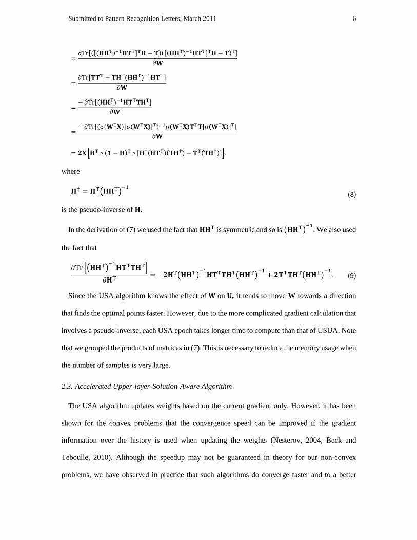
where
( )
(8)
is the pseudo-inverse of .
In the derivation of (7) we used the fact that is symmetric and so is ( )
. We also used
the fact that
[( ) ]
( )
( )
( )
(9)
Since the USA algorithm knows the effect of on , it tends to move W towards a direction
that finds the optimal points faster. However, due to the more complicated gradient calculation that
involves a pseudo-inverse, each USA epoch takes longer time to compute than that of USUA. Note
that we grouped the products of matrices in (7). This is necessary to reduce the memory usage when
the number of samples is very large.
2.3. Accelerated Upper-layer-Solution-Aware Algorithm
The USA algorithm updates weights based on the current gradient only. However, it has been
shown for the convex problems that the convergence speed can be improved if the gradient
information over the history is used when updating the weights (Nesterov, 2004, Beck and
Teboulle, 2010). Although the speedup may not be guaranteed in theory for our non-convex
problems, we have observed in practice that such algorithms do converge faster and to a better

Submitted to Pattern Recognition Letters, March 2011 7
place, we have observed in practice that such algorithms do converge faster and to a better place.
Actually, similar but less principled techniques such as momentum (Negnevitsky and Ringrose
1999) have been successfully applied to train non-convex multi-layer perceptrons (MLPs). In this
paper, we used the FISTA algorithm (Beck and Teboulle, 2010) to accelerate the learning process.
More specifically, we choose and set and during initialization. We then
update , and according to
(10)
( √
) (11)
( ) (12)
We name this algorithm accelerated USA (A-USA).
Note that since the A-USA algorithm needs to keep track of two sets of weights and , it is
slightly slower than the USA algorithm for each epoch. However, since it used the gradient
information from the history to determine the search direction, it can find the optimal solution with
less epochs than the USA algorithm. Additional information on how FISTA and similar techniques
can speed up the gradient descent algorithm can be found in (Nesterov, 2004, Beck and Teboulle,
2010).
2.4. Weighted Accelerated USA Algorithm
In (7), each sample is weighted the same. It is intuitive, however, that we may improve the
convergence speed by focusing on the samples with most errors for two reasons. First, it allows the
training procedure to slightly change the search direction (since weighted sum is different) at each
epoch and thus has better chance to jump out of the local optimums. Second, since the training
procedure focuses on the samples with most errors, it can reduce the overall errors faster.
In this work, we define the weight

Submitted to Pattern Recognition Letters, March 2011 8
‖ ‖
(
‖ ‖
) ( )⁄ (13)
for each sample , where is the square error over the whole training set, is the training set size,
and is a smoothing factor. The weighting factors are so chosen that they are positively
correlated to the errors introduced by each sample while being smoothed to make sure weights
assigned to each sample is at least ( )⁄ . is typically set to 1 initially and increases over
epochs so that eventually the original criterion defined in (1) is optimized.
At each step, instead of minimizing directly we can minimize the weighted error
[( ) ( ) ] (14)
where [ ] is an by diagonal weight matrix.
To minimize , once the lower-layer weights are fixed the upper-layer weights can be
determined by setting the gradient
[( ) ( ) ]
( )
(15)
to zero, which has the closed-form solution
( ) (16)
By plugging (16) into (14) and using similar derivation steps used to derive
in (7), we obtain
the gradient
[( ) ( ) ]
[([( ) ] ) ([( ) ] ) ]
[ ( ) ]
[( ) ]
[ ( ) [ ( )( ) ( )]]
(17)
where

Submitted to Pattern Recognition Letters, March 2011 9
( ) (18)
Note that since we re-estimate the weights after each epoch, the algorithm will try to move the
weights with a larger step toward the direction where the error can be most effectively reduced.
Once the error for a sample is reduced, the weight for that sample becomes smaller in the next
epoch. This not only speeds up the convergence but also makes the training less likely to be trapped
into local optima. Because this algorithm uses adaptive weightings, we name it weighted
accelerated USA (WA-USA).
3. EXPERIMENTS
We evaluated and compared the four learning algorithms described in Section 2 against the basic
ELM algorithm and the EI-ELM algorithm on the MNIST dataset (LeCun et al. 1998) and the
MAGIC gamma telescope dataset (Frank and Asuncion 2010).
3.1. Dataset Description
The MNIST dataset contains binary images of handwritten digits. The digits have been
size-normalized to fit in a 20x20 pixel box while preserving their aspect ratio and centered in a
28x28 image by computing and translating the center of mass of the pixels. The task is to classify
each 28x28 image into one of the 10 digits. The MNIST training set is composed of 60,000
examples from approximately 250 writers, out of which we randomly selected 5,000 samples as the
cross validation set. The test set has 10,000 patterns. The sets of writers of the training set and test
set are disjoint.
The MAGIC gamma telescope dataset was generated using the Monte Carlo procedure to
simulate registration of high energy gamma particles in a ground-based atmospheric Cherenkov
gamma telescope using the imaging technique. Cherenkov gamma telescope observes high energy
gamma rays, taking advantage of the radiation emitted by charged particles produced inside the
electromagnetic showers initiated by the gammas, and developing in the atmosphere. This
Cherenkov radiation leaks through the atmosphere and gets recorded in the detector, allowing
Submitted to Pattern Recognition Letters, March 2011 10
reconstruction of the shower parameters.
The MAGIC dataset contains 19020 samples out of which we randomly selected 10% (1902
samples) as the cross validation set, 10% (1902 samples) as the test set, and the rest as the training
set. Each sample in the dataset has 10 real-valued attributes and a class label (signal or
background). The task is to classify the observation to either the signal class or background class
based on the attributes. Note that these attributes have some structures. However, in this study we
did not exploit these structures since our goal is not to achieve the best result on this dataset but
compare different algorithms proposed in the paper.
3.2. Experimental Results on MNIST
We compared the basic ELM algorithm, the EI-ELM algorithm, and all four algorithms
described in Section 2 with the number of hidden units in the set of {64, 128, 256, 512, 1024, 2048}
on the MNIST dataset. The results are summarized in Table I. We ran each configuration 10 times
and report the mean and standard deviations in test-set classification accuracy, training-set
classification accuracy, and training time. The test time only depends on the model size and is
summarized in Table II. Not surprisingly, the test time approximately doubles when the hidden
layer size (and model size) doubles.
For EI-ELM, we randomly generated 50 new configurations of weights at each step first. The one
with least square error (LSE) was selected and survived. We noticed, however, that if we added
only one hidden unit at each time, the training process can be very slow. To make the training speed
comparable to other algorithms discussed in this paper, we added 16 hidden units at each step.
For USUA and USA, we set the maximum number of epochs to 30 and used simple line search
that doubles or halves the learning rate so as to improve the training objective function. When the
learning rate is smaller than 1e-6 the algorithms stopped even if the maximum number of epoch
was not reached.
We did not use line search for A-USA and WA-USA. The learning rate used in A-USA was fixed

Submitted to Pattern Recognition Letters, March 2011 11
for all epochs and was set to 0.001. We used the learning rate of 0.0005 in WA-USA for all settings,
which is smaller than that used for A-USA since the update is expected to move with large steps
along some directions. The cross validation set is used to select the best configuration and to
determine when to stop training.
The results summarized in Table I can be compared from several perspectives. To make
observation easier, we plot the test set accuracy in Fig. 1. If we compare the accuracy across
different algorithms for the same number of hidden units, we can clearly see that all the algorithms
proposed in this paper significantly outperform ELM and EI-ELM. We also notice that from the
accuracy point of view, WA-USA performs best, followed by A-USA, which in turn performs
better than USA and USUA. If we compare the training time for the SHLNNs with the same
number of hidden units, we can indeed see that ELM takes considerably less time (about two orders
of magnitude) than all other algorithms. Note all the algorithms proposed in this paper significantly
outperform EI-ELM with similar training time. This is expected since EI-ELM only uses the 0-th
order information while all our algorithms used first-order gradient information. Among the
algorithms proposed in this paper, WA-USA and A-USA perform faster than USA since they are
accelerated algorithms.
These results can be examined from a different angle. Instead of comparing results with the same
network size, we can compare SHLNNs with the same test-set’s accuracy. From Fig. 1 and Table I
we see that the best average accuracy obtained using ELM is 94.68% with 2048 hidden units.
EI-ELM is only slightly better than ELM with an average accuracy of 94.78%. This is because
when the number of hidden units increases, random selection becomes less effective. This fact is
also indicated by smaller standard deviations as the number of hidden units increases in ELM.
However, using USUA, we obtained accuracy of 94.84% with only 1024 hidden units. This would
cut the test time by half. Further improvement is achieved when we use USA with accuracy of
94.78% using only 512 hidden units. For A-USA only 256 hidden units are needed to achieve
95.87% accuracy. Further, only 128 hidden units are needed to obtain comparable accuracy of

Submitted to Pattern Recognition Letters, March 2011 12
94.80% using WA-USA. In other words, WA-USA can achieve the same accuracy as ELM using
only 1/16 of the network size and test time. This is extremely favorable for practical usage since a
1/16 test time translates to 16 times more throughput. Also note that it takes only 155 seconds to
train a network with 128 hidden units using WA-USA. This is in comparison to 28.35 seconds
needed to train a 2048 hidden unit ELM model and 2,220 seconds for a 1024 hidden unit EI-EIM
model. If 2048 hidden units are used, we can obtain 98.55% average test set accuracy with
WA-USA, which is very difficult to obtain using ELM.
Note that we can consistently achieve 100% classification accuracy on the training set when we
use WA-USA with 1024 and more hidden units which is not the case when other algorithms are
used. This prevents further improvement on the classification accuracy on both training and test
sets even though square error continues to decline. This also explains the smaller gain when the
number of hidden units increases from 1024 to 2048 when WA-USA is used.
TABLE I
SUMMARY OF TEST SET ACCURACY, TRAINING SET ACCURACY, AND TRAINING TIME ON
MNIST DIGIT CLASSIFICATION TASK
Algorithm # hid units Test Acc (%) Train Acc (%) Training Time (s)
ELM 64 67.88±2.01 66.88±2.00 1.05±0.14
ELM 128 78.99±1.20 78.06±1.28 1.89±0.07
ELM 256 85.55±0.44 84.9±0.36 3.46±0.12
ELM 512 89.65±0.28 89.41±0.27 6.96±0.06
ELM 1024 92.65±0.21 92.85±0.13 13.8±0.07
ELM 2048 94.68±0.06 95.31±0.05 28.35±0.17
EI-ELM 64 73.68±0.87 72.84±0.57 147.59±0.88
EI-ELM 128 81.46±0.63 80.61±0.44 282.37±1.27
EI-ELM 256 86.74±0.40 86.2±0.30 550.13±11.17
EI-ELM 512 90.52±0.35 90.24±0.17 1069.73±6.27
EI-ELM 1024 92.92±0.14 93.23±0.10 2220.47±18.41
EI-ELM 2048 94.78±0.15 95.51±0.07 4629.67±91.81
USUA 64 84.78±1.42 84.27±1.49 99.13±3.03
USUA 128 88.42±1.05 88.06±1.10 177.81±5.86
USUA 256 90.73±0.46 90.82±0.5 347.35±14.83
USUA 512 93.24±0.39 93.79±0.47 681.88±20.04
USUA 1024 94.84±0.37 95.82±0.41 1323.04±64.35
USUA 2048 96.27±0.14 97.86±0.13 2643.73±84.18
USA 64 86.4±1.06 85.89±1.25 114.68±2.00

Submitted to Pattern Recognition Letters, March 2011 13
USA 128 89.81±0.76 89.62±0.87 221.1±3.37
USA 256 92.59±0.86 92.86±0.83 463.97±10.43
USA 512 94.87±0.35 95.58±0.46 1029.47±13.45
USA 1024 96.47±0.13 97.63±0.10 2471.36±10.35
USA 2048 97.39±0.07 98.95±0.07 7116.77±19.10
A-USA 64 90.12±1.66 89.98±1.82 88.1±5.81
A-USA 128 94.35±0.16 94.82±0.11 153.77±0.41
A-USA 256 95.87±0.13 96.64±0.11 320.9±0.33
A-USA 512 97.01±0.12 98.04±0.17 717.64±0.60
A-USA 1024 97.64±0.06 99.3±0.03 1727.17±1.89
A-USA 2048 98.02±0.08 99.87±0.01 4916.57±2.64
WA-USA 64 93.64±0.46 94.12±0.46 84.51±0.61
WA-USA 128 96.03+0.25 97.08±0.20 154.9±0.85
WA-USA 256 97.09±0.21 98.720.12 322.4±1.91
WA-USA 512 97.59±0.13 99.56±0.09 757.34±0.75
WA-USA 1024 98.45±0.12 100±0 1965.28±7.10
WA-USA 2048 98.55±0.11 100±0 5907.17±10.81
Fig. 1. The average test set accuracy as a function of the number of hidden units and different
learning algorithms on the MNIST dataset.
Our proposed algorithms also compare favorably over other SHLNN training algorithms
previous proposed. For example, with random initialization WA-USA can achieve 97.3% test set
accuracy using 256 hidden units. This result is better than 95.3% test set accuracy achieved using
SHLNN with 300 hidden units but trained using conventional back-propagation algorithm with
mean square error criterion (LeCun et al. 1998).
Furthermore, using the WA-USA algorithm and the single 2048 hidden layer weights initialized
with the restricted Boltzmann machine (RBM), we obtained average test set accuracy of 98.9%
which is slightly better than the 98.8% obtained using a 3-hidden-layer DBN initialized using RBM

Submitted to Pattern Recognition Letters, March 2011 14
(Hinton and Salakhutdinov, 2006) with significantly less training time.
TABLE II
TEST TIME AS A FUNCTION OF THE NUMBER OF HIDDEN UNITS ON MNIST DATASET
# hidden
units Test Time (s)
64 0.19±0.01
128 0.38±0.03
256 0.76±0.06
512 1.48±0.13
1024 2.65±0.10
2048 4.97±0.08
3.3. Experimental Results on MAGIC Dataset
Similar comparison experiments have been conducted on the MAGIC dataset. Fig. 2
summarizes and compares the classification accuracy using ELM, EI-ELM, USUA, USA, A-USA,
and WA-USA algorithms as a function of the number of hidden units. Although the relative
accuracy improvement is different from those observed in MNIST dataset, the accuracy curves
share the same basic trend as that in Fig. 1. We can see that, esp. when the number of hidden units is
small, the proposed algorithms significantly outperform ELM and EI-ELM. Although when the
number of hidden units increases to 256, the gap between the accuracies obtained using proposed
approaches and that achieved using ELM and EI-ELM decreases, the difference is still very large.
Actually, ELM obtained the highest test set accuracy of 87.0% when 1024 hidden units are used
and when 2048 hidden units are used, it overfits the training data and the test set accuracy becomes
lower. However, we can achieve same or higher accuracies as the best achievable using ELM
algorithm with 64, 32, and 32 hidden units, respectively, using USA, A-USA, and WA-USA
algorithms. This indicates that at test time we can achieve the same or higher accuracy with 1/16,
1/32, and 1/32 of computation time using these algorithms compared to the ELM algorithm. Note
that to train a 32-hidden-unit SHLNN using the A-USA or WA-USA algorithm we only need to
spend less than four times of the time needed to train a 1024 hidden unit model using ELM.

Submitted to Pattern Recognition Letters, March 2011 15
Fig. 2. The average test set accuracy as a function of the number of hidden units and different
learning algorithms on the MAGIC dataset.
4. CONCLUSION
In this paper we presented four efficient algorithms for training SHLNNs. These algorithms
exploit information such as the structure of SHLNNs and gradient values over epochs, and update
the weights along the most promising direction. We demonstrated both the efficiency and
effectiveness of these algorithms on the MNIST and MAGIC datasets. Among all the algorithms
developed in this work, we recommend using the WA-USA and A-USA algorithms since they
converge fastest and typically to a better model. We believe this line of work can help improve the
scalability of neural networks in speech recognition systems (e.g., Dahl et al. 2012, Yu and Deng
2010) which typically require thousands of hours of training data.
ACKNOWLEDGMENT
We thank Dr. Guang-Bin Huang at Singapore Nanyang Technological University for fruitful
discussions on ELM.
70%
72%
74%
76%
78%
80%
82%
84%
86%
88%
90%
8 16 32 64 128 256
Acc
ura
cy
Number of Hidden Units
ELM
EI-ELM
USUA
USA
A-USA
WA-USA

Submitted to Pattern Recognition Letters, March 2011 16
REFERENCES
[1] Beck, A. and Teboulle, M. (2010) “Gradient-based methods with application to signal recovery
problems," Convex Optimization in Signal Processing and Communications, D. Palomar and
Y. Eldar (Eds.), Cambridge University Press.
[2] Dahl, G. E., Yu, D., Deng, L. and Acero, A. (2012) "Context-dependent pre-trained deep neural
networks for large vocabulary speech recognition", IEEE Transactions on Audio, Speech, and
Language Processing - Special Issue on Deep Learning for Speech and Language Processing.
[3] Frank, A. & Asuncion, A. (2010). UCI Machine Learning Repository
[http://archive.ics.uci.edu/ml]. Irvine, CA: University of California, School of Information and
Computer Science.
[4] Hinton, G. E. and Salakhutdinov, R. R. (2006) “Reducing the dimensionality of data with
neural networks”, Science, Vol. 313. no. 5786, pp. 504 - 507.
[5] Hoerl, A. E. and Kennard, R. W. (1970) “Ridge regression: biased estimation for
nonorthogonal problems”, Technometrics, vol. 12, no. 1, pp. 55-67.
[6] Huang, G.-B., Zhu, Q.-Y. and Siew, C.-K. (2006) “Extreme learning machine: theory and
applications”, Neurocomputing, vol. 70, pp. 489-501.
[7] Huang, G.-B. and Chen, L. (2008) “Enhanced random search based incremental extreme
learning machine,” Neurocomputing, vol. 71, pp. 3460-3468.
[8] LeCun, Y., Bottou, L., Bengio, Y. and Haffner, P. (1998) “Gradient-based learning applied to
document recognition”, Proceedings of the IEEE, 86(11):2278-2324.
[9] Negnevitsky, M., Ringrose, M. (1999) "Accelerated learning in multi-layer neural networks ",
Neural Information Processing, 1999, ICONIP, Vol. 3, pp 1167 – 1171.
[10] Nesterov, Y. (2004) Introductory Lectures on Convex Optimization: A Basic Course, Kluwer
Academic Publishers.

Submitted to Pattern Recognition Letters, March 2011 17
[11] Yu, D. and Deng, L. (2011) "Deep learning and its relevance to signal and information
processing", IEEE Signal Processing Magazine, vol. 28, No. 1, pp. 145-154.
[12] Zhu, Q.-Y., Qin, A. K., Suganthan, P. N. and Huang, G.-B. (2005) “Evolutionary extreme
learning machine,” Pattern Recognition, vol. 38, pp. 1759-1763.