efficient and safe global constraints for handling · efficient and safe global constraints 2077...

EFFICIENT AND SAFE GLOBAL CONSTRAINTS FOR HANDLINGNUMERICAL CONSTRAINT SYSTEMS∗

YAHIA LEBBAH†¶, CLAUDE MICHEL‡¶, MICHEL RUEHER‡¶, DAVID DANEY§¶, AND

JEAN-PIERRE MERLET§¶

SIAM J. NUMER. ANAL. c© 2005 Society for Industrial and Applied MathematicsVol. 42, No. 5, pp. 2076–2097

Abstract. Numerical constraint systems are often handled by branch and prune algorithms thatcombine splitting techniques, local consistencies, and interval methods. This paper first recalls theprinciples of Quad, a global constraint that works on a tight and safe linear relaxation of quadraticsubsystems of constraints. Then, it introduces a generalization of Quad to polynomial constraintsystems. It also introduces a method to get safe linear relaxations and shows how to computesafe bounds of the variables of the linear constraint system. Different linearization techniques areinvestigated to limit the number of generated constraints. QuadSolver, a new branch and prunealgorithm that combines Quad, local consistencies, and interval methods, is introduced. QuadSolver

has been evaluated on a variety of benchmarks from kinematics, mechanics, and robotics. On thesebenchmarks, it outperforms classical interval methods as well as constraint satisfaction problemsolvers and it compares well with state-of-the-art optimization solvers.

Key words. systems of equations and inequalities, constraint programming, reformulationlinearization technique, global constraint, interval arithmetic, safe rounding

AMS subject classifications. 65H10, 65G40, 65H20, 93B18, 65G20

DOI. 10.1137/S0036142903436174

1. Introduction. Many applications in engineering sciences require finding allisolated solutions to systems of constraints over real numbers. These systems maybe nonpolynomial and are difficult to solve: the inherent computational complexityis NP-hard and numerical issues are critical in practice (e.g., it is far from beingobvious to guarantee correctness and completeness as well as to ensure termination).These systems, called numerical CSP (constraint satisfaction problem) in the restof this paper, have been approached in the past by different interesting methods:1

interval methods [35, 24, 38, 20, 40], continuation methods [37, 2, 62], and constraintsatisfaction methods [30, 6, 11, 61]. Of particular interest is the mathematical andprogramming simplicity of the latter approach: the general framework is a branch andprune algorithm that requires only specifying the constraints and the initial range ofthe variables.

The purpose of this paper is to introduce and study a new branch and boundalgorithm called QuadSolver. The essential feature of this algorithm is a globalconstraint—called Quad—that works on a tight and safe linear relaxation of the poly-nomial relations of the constraint systems. More precisely, QuadSolver is a branch

∗Received by the editors October 15, 2003; accepted for publication (in revised form) June 3,2004; published electronically February 25, 2005.

http://www.siam.org/journals/sinum/42-5/43617.html†Departement Informatique, Faculte des Sciences, Universite d’Oran Es-Senia, BP 1524, El-

M’Naouar Oran, Algeria ([email protected]).‡Universite de Nice-Sophia Antipolis, I3S-CNRS, 930 route des Colles, BP 145, 06903 Sophia

Antipolis Cedex, France ([email protected], [email protected]).§INRIA, 2004 route des Lucioles, BP 93, 06902 Sophia Antipolis Cedex, France (David.Daney@

sophia.inria.fr, [email protected]).¶COPRIN Project INRIA–I3S–CNRS, 2004 route des Luciales, BP 93, Sophia Antipolis Cedex

06903, France.1Alternative methods have been proposed for solving nonlinear systems. For instance, algebraic

constraints can be handled with symbolic methods [13] (e.g., Groebner basis, resultant). However,these methods can neither handle nonpolynomial systems nor deal with inequalities.

2076

EFFICIENT AND SAFE GLOBAL CONSTRAINTS 2077

and prune algorithm that combines Quad, local consistencies, and interval methods.That is to say, QuadSolver is an attempt to merge the best interval and constraintprogramming techniques. QuadSolver has been evaluated on a variety of benchmarksfrom kinematics, mechanics, and robotics. On these benchmarks, it outperforms clas-sical interval methods as well as CSP solvers and it compares well with state-of-the-artoptimization solvers.

The Quad-filtering algorithm [27] has first been defined for quadratic constraints.The relaxation of quadratic terms is adapted from a classical linearization method,the reformulation-linearization technique (RLT) [54, 53]. The simplex algorithm isused to narrow the domain of each variable with respect to the subset of the linearset of constraints generated by the relaxation process. The coefficients of these linearconstraints are updated with the new values of the bounds of the domains and theprocess is restarted until no more significant reduction can be done. We have demon-strated [27] that the Quad algorithm yields a more effective pruning of the domainsthan local consistency filtering algorithms (e.g., 2b-consistency [30] or box-consistency[6]). Indeed, the drawback of classical local consistencies comes from the fact that theconstraints are handled independently and in a blind way.2 That is to say, classicallocal consistencies do not exploit the semantic of quadratic terms; in other words,these approaches do not take advantage of the very specific semantic of quadraticconstraints to reduce the domains of the variables. Conversely, linear programmingtechniques [1, 54, 3] do capture most of the semantics of quadratic terms, e.g., convexand concave envelopes of these particular terms.3

The extension of Quad for handling any polynomial constraint system requiresreplacing nonquadratic terms by new variables and adding the corresponding identi-ties to the initial constraint system. However, a complete quadrification [58] wouldgenerate a huge number of linear constraints. Thus, we introduce here an heuristicbased on a good tradeoff between a tight approximation of the nonlinear terms andthe size of the generated constraint system. This heuristic works well on classicalbenchmarks (see section 8).

A safe rounding process is a key issue for the Quad framework. Let us recall thatthe simplex algorithm is used to narrow the domain of each variable with respect tothe subset of the linear set of constraints generated by the relaxation process. Thepoint is that most implementations of the simplex algorithm are unsafe. Moreover,the coefficients of the generated linear constraints are computed with floating pointnumbers. So, two problems may occur in the Quad-filtering process.

1. The whole linearization may become incorrect due to rounding errors whencomputing the coefficients of the generated linear constraints.

2. Some solutions may be lost when computing the bounds of the domains ofthe variables with the simplex algorithm.

We propose in this paper a safe procedure for computing the coefficients of thegenerated linear constraints. Neumaier and Shcherbina [42] have addressed the second

23b-consistency and kb-consistency are partial consistencies that can achieve a better pruningsince they are “less local” [11]. However, they require numerous splitting steps to find the solutionsof a system of quadratic constraints; so, they may become rather slow.

3Sherali and Tuncbilek [55] have also proposed four different filtering techniques for solvingquadratic problems. Roughly speaking, the first filtering strategy performs a feasibility check oninequality constraints to discard subintervals of the domains of the variables. This strategy is veryclose to box-consistency filtering (see [60]). The three other techniques are based on specific propertiesof optimization problems with a quadratic objective function: the eigenstructure of the quadraticobjective function, fathoming node, and Lagrangian dual problem. Thus, these techniques can beconsidered as local consistencies for optimization problems (see also [59] and Neumaier’s survey [41]).

2078 LEBBAH, MICHEL, RUEHER, DANEY, AND MERLET

problem.4 They have proposed a simple and cheap procedure to get a rigorous upperbound of the objective function. The incorporation of these procedures in the Quad-filtering process allows us to call the simplex algorithm without worrying about safety.So, with these two procedures, linear programming techniques can be used to tacklecontinuous CSPs without losing any solution.

The rest of this paper is organized as follows. Section 2 gives an overview of theapproach whereas section 3 contains the notation. Sections 4 and 5 recall the basicsof interval programming and constraint programming. Section 6 details the principleof the Quad algorithm, the linearization process, and the extension to polynomialconstraints. Section 7 introduces the rounding process we propose to ensure the saferelaxations. Section 8 describes the experimental results and discusses related work.Concluding remarks are given in section 9.

2. Overview of the approach. As mentioned, QuadSolver is a branch andprune algorithm that combines Quad and a box-consistency.

Box-consistency is the most successful adaptation of arc-consistency [31] toconstraints over the real numbers. The box-consistency implementation of Van-Hentenryck, McAllester, and Kapur [60] is computed on three-interval extensionsof the initial constraints: the natural interval extension, the distributed interval ex-tension, and the Taylor interval extension with a conditioning step. The leftmost andthe rightmost zeros are computed using a variation of the univariate interval Newtonmethod.

The QuadSolver we propose here combines Quad-filtering and box-consistencyfiltering to prune the domain of the variables of numerical constraint systems. Oper-ationally, QuadSolver performs the following filtering processes:

1. box-consistency filtering,2. Quad-filtering.

The box-consistency is first used to detect some inconsistencies before startingthe Quad-filtering algorithm which is more costly. These two steps are wrapped into aclassical fixed point algorithm which stops when the domains of the variables cannotbe further reduced.5

To isolate the different solutions, Quad uses classical branching techniques.Before going into the details, let us outline the advantages of our approach on a

couple of small examples.

2.1. Quad-filtering. Consider the constraint system C = {2xy+y = 1, xy = 0.2}which represents two intersecting curves (see Figure 2.1). Suppose that x = [−10,+10]and y = [−10,+10] are the domains of the variables x and y. An interval x = [x, x]denotes the set of reals {r|x ≤ r ≤ x}.

The RLT (see section 6.2) yields the following constraint system:⎧⎪⎪⎨⎪⎪⎩

y + 2w = 1, w = 0.2,yx + xy − w ≤ xy, yx + xy − w ≥ xy,yx + xy − w ≥ xy, yx + xy − w ≤ xy,x ≥ x, x ≤ x, y ≥ y, y ≤ y,

(a)

where w is a new variable that stands for the product xy. Note that constraint system(a) implies that w ∈ [x, x] ∗ [y, y].

4They have also suggested a solution to the first problem though their solution is dedicated tomixed integer programming problems.

5In practice, the loop stops when the domain reduction is lower than a given ε.


0

y

x

Fig. 2.1. Geometrical representation of {2xy + y = 1, xy = 0.2}.

Substituting x, y, x, and y by their values and minimizing (resp., maximizing) x, y,and w with the simplex algorithm yield the following new bounds:

x = [−9.38, 9.42], y = [0.6, 0.6], w = [0.2, 0.2].

By substituting the new bounds of x, y, and w in the constraint system (a), we ob-tain a new linear constraint system. One more minimizing (resp., maximizing) stepis required to obtain tight bounds of x. Note that numerous splitting operations arerequired to find the unique solution of the problem with a 3b-consistency filteringalgorithm. The proposed algorithm solves the problem by generating 6 linear con-straints and with 8 calls to the simplex algorithm. It finds the same solution as asolver based on 3b-consistency but without splitting and in less time.

2.2. A safe rounding procedure. Consider the constraint system

C =

{w1 + w2 = 1, w1x1 + w2x2 = 0,w1x1x1 + w2x2x2 = 1, w1x1x1x1 + w2x2x2x2 = 0,

which represents a simple Gaussian quadrature formula to compute integrals [9]. Sup-pose that the domains of variables x1, x2, w1, and w2 are all equal to [−1,+1]. Thissystem has two solutions:

• x1 = −1, x2 = 1, w1 = 0.5, w2 = 0.5,• x1 = 1, x2 = −1, w1 = 0.5, w2 = 0.5.

A straightforward implementation of Quad would only find one unsafe solutionwith

x2 ∈ [+0.9999 . . . 944,+0.9999 . . . 989].

Indeed, when we examine the Quad-filtering process, we can identify some linear pro-grams where the simplex algorithm steps to the wrong side of the objective.

With the corrections we propose in section 7, we obtain a tight approximationof the two correct solutions (with x2 ∈ [−1.000000 . . . ,−0.999999 . . . ] and x2 ∈[0.999999 . . . , 1.000000 . . . ]).

3. Notation and basic definitions. This paper focuses on CSPs where thedomains are intervals and the constraints Cj(x1, . . . , xn) are n-ary relations over thereals. C stands for the set of constraints.

x or Dx denotes the domain of variable x, that is to say, the set of allowed valuesfor x. D stands for the set of domains of all the variables of the considered constraint


system. R denotes the set of real numbers whereas F stands for the set of floatingpoint numbers used in the implementation of nonlinear constraint solvers; if a is aconstant in F, a+ (resp., a−) corresponds to the smallest (resp., largest) number of F

strictly greater (resp., lower) than a.x = [x, x] is defined as the set of real numbers x verifying x ≤ x ≤ x. x, y denote

real variables, X,Y denote vectors whereas X,Y denote interval vectors. The widthw(x) of an interval x is the quantity x − x while the midpoint m(x) of the intervalx is (x + x)/2. A point interval x is obtained if x = x. A box is a set of intervals:its width is defined as the largest width of its interval members, while its center isdefined as the point whose coordinates is the midpoint of the ranges. IR

n denotes theset of boxes and is ordered by set inclusion.

We use the RLT notation introduced in [54, 3] with slight modifications. Moreprecisely, we will use the following notations: [c]L is the set of linear constraintsgenerated by replacing the nonlinear terms by new variables in constraint c, and [c]LI

denotes the set of equations that keep the link between the new variables and thenonlinear terms while [c]R contains linear inequalities that approximate the semanticsof nonlinear terms of constraint c. These notations will be used indifferently whetherc is a constraint or C is a set of constraints.

Rounding is necessary to close the operations over F (see [18]). A rounding func-tion maps the result of the evaluation of an expression to available floating-point num-bers. Rounding x towards +∞ maps x to the least floating point number xf such thatx ≤ xf . �(x) (resp., �(x)) denotes a rounding mode of x towards −∞ (resp., +∞).

4. Interval programming. This section recalls the basic concepts of intervalarithmetic that are required to understand the rest of the paper. Readers familiarwith interval arithmetic may skip this section.

4.1. Interval arithmetic. Interval arithmetic has been introduced by Moore [35].It is based on the representation of variables as intervals.

Let f be a real-valued function of n unknowns X = (x1, . . . , xn). An intervalevaluation of f for given ranges X = (x1, . . . ,xn) for the unknowns is an interval ysuch that

y ≤ f(X) ≤ y for all X = (x1, . . . , xn) ∈ X = (x1, . . . ,xn).(4.1)

In other words, y and y are lower and upper bounds for the values of f when thevalues of the unknowns are restricted to the box X.

There are numerous ways to calculate an interval evaluation of a function [20, 46].The simplest is the natural evaluation in which all the mathematical operators in fare substituted by their interval equivalents. Interval equivalents exist for all classicalmathematical operators. Hence interval arithmetic allows us to calculate an intervalevaluation for all nonlinear expressions, whether algebraic or not. For example, iff(x) = x + sin(x), then the interval evaluation of f for x ∈ [1.1, 2] can be calculatedas follows:

f([1.1, 2]) = [1.1, 2] + sin([1.1, 2]) = [1.1, 2] + [0.8912, 1] = [1.9912, 3].

Interval arithmetic can be implemented with directed rounding to take into ac-count round-off errors. There are numerous interval arithmetic packages implementingthis property: one of the most famous library is BIAS/Profil,6 but a promising new

6http://www.ti3.tu-harburg.de/Software/PROFILEnglisch.html.


package—based on the multiprecision software MPFR7—is MPFI [47].The main limitation of interval arithmetic is the overestimation of interval func-

tions. This is due to two well-known problems:• the so-called wrapping effect [35, 39], which overestimates by a unique vector

the image of an interval vector (which is in general not a vector). That is tosay, {f(X)|X ∈ X} is contained in f(X) but is usually not equal to f(X);

• the so-called dependency problem [20], which is due to the independence ofthe different occurrences of some variables during the interval evaluation ofan expression. In other words, during the interval evaluation process thereis no correlation between the different occurrences of a same variable in anequation. For instance, consider x = [0, 10]. x−x = [x−x, x−x] = [−10, 10]instead of [0, 0] as one could expect.

In general, it is not possible to compute the exact enclosure of the range for anarbitrary function over the real numbers [25]. Thus, Moore introduced the conceptof interval extension: the interval extension of a function is an interval function thatcomputes outer approximations on the range of the function over a domain [20, 36].Two main extensions have been introduced: the natural extension and the Taylorextension [46, 20, 38].8 Due to the properties of interval arithmetic, the evaluation ofa function may yield different results according to the literal form of the equations.Thus, many literal forms may be used as, for example, factorized form (Horner forpolynomial system) or distributed form [60].

Nevertheless, in general, neither the natural form nor the Taylor expansion allowsus to compute the exact range of a function f . For instance, considering f(x) =1 − x + x2 and x = [0, 2], we have

ftay([0, 2]) = f(x) + (2x − 1)(x − x) = f(1) + (2[0, 2] − 1)([0, 2] − 1) = [−2, 4],

f([0, 2]) = 1 − x + x2 = 1 − [0, 2] + [0, 2]2 = [−1, 5],(4.2)

ffactor([0, 2]) = 1 + x(x − 1) = 1 + [0, 2]([0, 2] − 1) = [−1, 3],

whereas the range of f over X = [0, 2] is [3/4, 3]. In this case, this result could directlybe obtained by a second form of factorization: ffactor2([0, 2]) = (x − 1/2)2 + 3/4 =([0, 2] − 1/2)2 + 3/4 = [3/4, 3].

4.2. Interval analysis methods. This section provides a short introductionto interval analysis methods (see [35, 20, 38, 40] for a more detailed introduction).We limit this overview to interval Newton-like methods for solving a multivariatesystem of nonlinear equations. Their use is complementary to methods provided bythe constraint programming community.

The aim is to determine the zeros of a system of n equations fi(x1, . . . , xn) in nunknowns xi inside the interval vector X = (x1, . . . ,xn) with xi ∈ xi for i = 1, . . . , n.

First, consider solving an interval linear system of equations defined as follows:

AX = b, A ∈ A, b ∈ b,(4.3)

where A is an interval matrix and b is an interval vector. Solving this linear intervalsystem requires us to determine an interval vector X containing all solutions of allscalar linear systems noted AX = b such that A ∈ A and b ∈ b. Finding the exactvalue of X is a difficult problem, but three basic interval methods exist: Gaussian

7http://www.mpfr.org.8ftay(X) = f(X) + A(X −X), where A is the Jacobian or the interval slope matrix.


elimination, Gauss–Seidel iterative method, or Krawczyk method (see [24, 38, 20, 40]).They may provide an overestimated interval vector X1 including X. However, ingeneral the computed intervals are too wide and a preconditioning is required, thatis to say, a multiplication of both sides of (4.3) by the inverse of a midpoint of A.The matrix m(A)−1A is then “closer” to the identity matrix and the width of X1 issmaller [20].

To solve nonlinear systems, an interval Newton algorithm is often used—see[20] or [38]. The basic idea is to solve iteratively a linear approximation of thenonlinear system obtained by a Taylor expansion. Many improvements [24, 19], basedon variations of the resolution of the linear subsystem or the preconditioning, havebeen proposed. Note that many interesting properties are provided by Newton-likemethods: existence and/or uniqueness of a root, convergence area/rate, . . . .

5. Constraint programming. This section recalls the basics of constraint pro-gramming techniques which are required to understand the rest of this paper. Adetailed discussion of these concepts and techniques can be found in [6, 26].

5.1. The general framework. The constraint programming framework is basedon a branch and prune scheme which was inspired by the traditional branch and boundapproach used in optimization problems. That is to say, it is best viewed as an itera-tion of two steps [60]:

1. pruning the search space;2. making a choice to generate two (or more) subproblems.

The pruning step ensures that some local consistency holds. In other words, thepruning step reduces an interval when it can prove that the upper bound or the lowerbound does not satisfy some constraint. Informally speaking, a constraint system Csatisfies a partial consistency property if a relaxation of C is consistent. For instanceconsider x = [x, x] and c(x, x1, . . . , xn) ∈ C. Whenever c(x, x1, . . . , xn) does not holdfor any values a ∈ x = [x, x′], then x may be shrunk to x = [x′, x]. Local consistenciesare detailed in the next subsection. Roughly speaking, they are relaxations of arc-consistency, a notion that is well known in artificial intelligence [31, 34].

The branching step usually splits the interval associated to some variable in twointervals with the same width. However, the splitting process may generate more thantwo subproblems and one may split an interval at a point different from its midpoint.The choice of the variable to split is a critical issue in difficult problems. Sophisticatedsplitting strategies have been developed for finite domains but few results [23] areavailable for continuous domains.

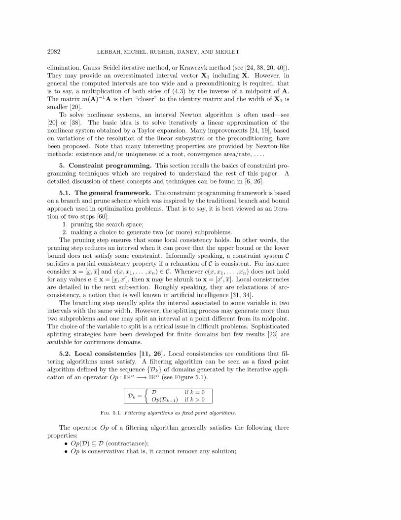
5.2. Local consistencies [11, 26]. Local consistencies are conditions that fil-tering algorithms must satisfy. A filtering algorithm can be seen as a fixed pointalgorithm defined by the sequence {Dk} of domains generated by the iterative appli-cation of an operator Op : IR

n −→ IRn (see Figure 5.1).

Dk =

{D if k = 0Op(Dk−1) if k > 0

Fig. 5.1. Filtering algorithms as fixed point algorithms.

The operator Op of a filtering algorithm generally satisfies the following threeproperties:

• Op(D) ⊆ D (contractance);• Op is conservative; that is, it cannot remove any solution;


• D′ ⊆ D ⇒ Op(D′) ⊆ Op(D) (monotonicity).

Under those conditions, the limit of the sequence {Dk}, which corresponds to thegreatest fixed point of the operator Op, exists and is called a closure. A fixed pointfor Op may be characterized by an lc-consistency property, called a local consistency.The algorithm achieving filtering by lc-consistency is denoted lc-filtering. A CSP issaid to be lc-satisfiable if lc-filtering of this CSP does not produce an empty domain.

Consistencies used in numerical CSP solvers can be categorized in two mainclasses: arc-consistency-like consistencies and strong consistencies. Strong consis-tencies will not be discussed in this paper (see [30, 26] for a detailed introduction).

Most of the numerical CSP systems (for example, BNR-prolog [43], Interlog [8],CLP(BNR) [7], PrologIV [12], UniCalc [4], Ilog Solver [22], Numerica [61], andRealPaver [5]) compute an approximation of arc-consistency [31] which will be namedac-like-consistency in this paper. An ac-like-consistency states a local property on aconstraint and on the bounds of the domains of its variables. Roughly speaking, aconstraint cj is ac-like-consistent if for any variable xi in var(cj), the bounds xi andxi have a support in the domains of all other variables of cj .

The most famous ac-like consistencies are 2b-consistency and box-consistency.

2b-consistency (also known as hull consistency) [10, 7, 28, 30] requires only tocheck the arc-consistency property for each bound of the intervals. The key point isthat this relaxation is more easily verifiable than arc-consistency itself. Informallyspeaking, variable x is 2b-consistent for constraint “f(x, x1, . . . , xn) = 0” if the lower(resp., upper) bound of the domain of x is the smallest (resp., largest) solution off(x, x1, . . . , xn). The box-consistency [6, 21] is a coarser relaxation (i.e., it allows lessstringent pruning) of arc-consistency than 2b-consistency. Variable x is box-consistentfor constraint “f(x, x1, . . . , xn) = 0” if the bounds of the domain of x correspond tothe leftmost and rightmost zeros of the optimal interval extension of f(x, x1, . . . , xn).2b-consistency algorithms actually achieve a weaker filtering (i.e., a filtering thatyields bigger intervals) than box-consistency, more precisely when a variable occursmore than once in some constraint (see Proposition 6 in [11]). This is due to thefact that 2b-consistency algorithms require a decomposition of the constraints withmultiple occurrences of the same variable.

2b-consistency [30] states a local property on the bounds of the domains of avariable at a single constraint level. A constraint c is 2b-consistent if, for any variablex, there exist values in the domains of all other variables which satisfy c when x isfixed to x and x.

The filtering by 2b-consistency of P = (D, C) is the CSP P ′ = (D′, C) such that

• P and P ′ have the same solutions;• P ′ is 2b-consistent;• D′ ⊆ D and the domains in D′ are the largest ones for which P ′ is 2b-

consistent.

Filtering by 2b-consistency of P always exists and is unique [30], that is to say it is aclosure.

The box-consistency [6, 21] is a coarser relaxation of arc-consistency than 2b-consistency. It mainly consists of replacing every existentially quantified variablebut one with its interval in the definition of 2b-consistency. Thus, box-consistencygenerates a system of univariate interval functions which can be tackled by numericalmethods such as interval Newton. In contrast to 2b-consistency, box-consistencydoes not require any constraint decomposition and thus does not amplify the localityproblem. Moreover, box-consistency can tackle some dependency problems when each


constraint of a CSP contains only one variable which has multiple occurrences. Moreformally we have the following definition.

Definition 5.1 (box-consistency). Let (D, C) be a CSP and c ∈ C a k-ary con-straint over the variables (x1, . . . , xk). c is box-consistent if, for all xi, the followingrelations hold:

1. c(x1, . . . ,xi−1, [xi, x+i ),xi+1, . . . ,xk),

2. c(x1, . . . ,xi−1, (x−i , xi],xi+1, . . . ,xk).

Closure by box-consistency of P is defined similarly as closure by 2b-consistencyof P .

Benhamou et al. have introduced HC4 [5], an ac-like-consistency that merges2b-consistency and box-consistency and which optimizes the computation process.

6. Quad basics and extensions. This section first introduces Quad, a globalconstraint that works on a tight and safe linear relaxation of quadratic subsystems ofconstraints. Then, it generalizes Quad to the polynomial part of numerical constraintsystems. Different linearization techniques are investigated to limit the number ofgenerated constraints.

6.1. The Quad algorithm. The Quad-filtering algorithm (see Algorithm 1) con-sists of three main steps: reformulation, linearization, and pruning.

The reformulation step generates [C]R, the set of implied linear constraints. Moreprecisely, [C]R contains linear inequalities that approximate the semantics of nonlinearterms of C.

The linearization process first decomposes each nonlinear term in sums and prod-ucts of univariate terms; then it replaces nonlinear terms with their associated newvariables. For example, considering constraint c : x2x3x

24(x6 + x7) + sin(x1)(x2x6 −

x3) = 0, a simple linearization transformation may yield the following sets:

• [c]L = {y1 + y3 = 0, y2 = x6 + x7, y4 = y5 − x3},• [c]LI = {y1 = x2x3x

24y2, y3 = sin(x1)y4, y5 = x2x6}.

[c]L is the set of linear constraints generated by replacing the nonlinear terms bynew variables and [c]LI denotes the set of equations that keep the link between thenew variables and the nonlinear terms. Note that the nonlinear terms which are notdirectly handled by the Quad are taken into account by the box-filtering process.

Finally, the linearization step computes the set of final linear inequalities andequations LR = [C]L ∪ [C]R, the linear relaxation of the original constraints C.

The pruning step is just a fixed point algorithm that calls iteratively a linearprogramming solver to reduce the upper and lower bounds of every original variable.The algorithm converges and terminates if ε is greater than zero.

Now we are in the position to introduce the reformulation of nonlinear terms.Section 6.2 first introduces the handling of quadratic constraints while section 6.3extends the previous results to polynomial constraints.

6.2. Handling quadratic constraints. Quadratic constraints are approximatedby linear constraints in the following way. Quad creates a new variable for eachquadratic term: y for x2 and yi,j for xixj . The produced system is denoted as

⎡⎣ ∑

(i,j)∈M

ak,i,jxixj +∑i∈N

bk,ix2i +

∑i∈N

dk,ixi = bk

⎤⎦L

.

.


Function Quad filtering(IN: X , D, C, ε) return D′

% X : initial variables; D: input domains; C: constraints; ε: minimal reduction% D′: output domains

1. Reformulation: generation of linear inequalities [C]R for the nonlinear termsin C.

2. Linearization: linearization of the whole system [C]L.We obtain a linear system LR = [C]L ∪ [C]R.

3. D′ := D.

4. Pruning:While the amount of reduction of some bound is greater than ε and ∅ �∈ D′

Do

(a) D ← D′.(b) Update the coefficients of the linearizations [C]R according to the do-

mains D′.(c) Reduce the lower and upper bounds x′

i and x′i of each initial variable

xi ∈ X by computing min and max of xi subject to LR with a linearprogramming solver.

Algorithm 1

The Quad-algorithm.

A tight linear (convex) relaxation, or outer-approximation to the convex and con-cave envelope of the quadratic terms over the constrained region, is built by generatingnew linear inequalities.

Quad uses two tight linear relaxation classes that preserve equations y = x2 andyi,j = xixj and that provide a better approximation than interval arithmetic [27].

6.2.1. Linearization of x2. The term x2 with x ≤ x ≤ x is approximated bythe following relations:

[x2]R =

{L1(α) ≡ [(x− α)2 ≥ 0]L, where α ∈ [x, x],

L2 ≡ [(x + x)x− y − xx ≥ 0]L.(6.1)

Note that [(x − αi)2 = 0]L generates the tangent line to the curve y = x2 at the

point x = αi. Actually, Quad computes only L1(x) and L1(x). Consider for instancethe quadratic term x2 with x ∈ [−4, 5]. Figure 6.1 displays the initial curve (i.e.,D1) and the lines corresponding to the equations generated by the relaxations: D2

for L1(−4) ≡ y + 8x + 16 ≥ 0, D3 for L1(5) ≡ y − 10x + 25 ≥ 0, and D4 forL2 ≡ −y + x + 20 ≥ 0.

We may note that L1(x) and L1(x) are underestimations of x2 whereas L2 is anoverestimation. L2 is also the concave envelope, which means that it is the optimalconcave overestimation.

6.2.2. Bilinear terms. In the case of bilinear terms xy, McCormick [32] pro-posed the following relaxations of xy over the box [x, x]×[y, y], stated in the equivalentRLT form [54]:

[xy]R =

⎧⎪⎪⎨⎪⎪⎩

BIL1 ≡ [(x− x)(y − y) ≥ 0]L,BIL2 ≡ [(x− x)(y − y) ≥ 0]L,BIL3 ≡ [(x− x)(y − y) ≥ 0]L,BIL4 ≡ [(x− x)(y − y) ≥ 0]L.

(6.2)


D1D2,D3D4

0

y

x

Fig. 6.1. Approximation of x2.

CuD1, D3D2, D4

0

y

x

Fig. 6.2. Illustration of xy relaxations.

BIL1 and BIL3 define a convex envelope of xy whereas BIL2 and BIL4 define aconcave envelope of xy over the box [x, x] × [y, y]. Al-Khayyal and Falk [1] showedthat these relaxations are the optimal convex/concave outer-estimations of xy.

Consider for instance the quadratic term xy with x ∈ [−5, 5] and y ∈ [−5, 5].The work done by the linear relaxations of the three-dimensional curve z = xy is wellillustrated in two dimensions by fixing z. Figure 6.2 displays the two-dimensionalshape, for the level z = 5, of the initial curve (i.e., Cu) and the lines corresponding tothe equations generated by the relaxations (where z = 5): D1 for BIL1 ≡ z+5x+5y+25 ≥ 0, D2 for BIL2 ≡ −z+5x− 5y+25 ≥ 0, D3 for BIL3 ≡ −z− 5x+5y+25 ≥ 0,and D4 for BIL4 ≡ z − 5x− 5y + 25 ≥ 0.

6.3. Extension to polynomial constraints. In this section, we show howto extend the linearization process to polynomial constraints. We first discuss thequadrification process and compare it with RLT. Then, we present the linearizationsof product and power terms.

6.3.1. Transformation of nonlinear constraints into quadratic constraints.In this section, we show how to transform a polynomial constraint system into anequivalent quadratic constraint system, a process called quadrification [58].

For example, considering the constraint c : x2x3x24 + 3x6x7 + sin(x1) = 0, the

proposed transformation yields

{y1y2 + 3y2 + s1 = 0, y1 = x2x3, y2 = x4x4, y3 = x6x7}

and the set {y1 = x2x3, y2 = x24, y3 = x6x7, s1 = sin(x1)} of equations that keep

the link between the new variables and the nonlinear terms that cannot be furtherquadrified. Such a transformation is one of the possible quadrifications. It is called asingle quadrification.

We could generate all possible single quadrifications, or all quadrifying identities,and perform a so-called complete quadrification. For example, the complete quadrifi-cation of E = {x2x3x

24 + 3x6x7 + sin(x1) = 0} is⎧⎪⎪⎪⎪⎪⎪⎨

⎪⎪⎪⎪⎪⎪⎩

y1 + 3y2 + s1 = 0, y2 = x6x7,y1 = y3y4, y3 = x2x3, y4 = x2

4,y1 = y5y6, y5 = x2x4, y6 = x3x4,y1 = x2y7, y7 = x3y4, y7 = x4y6,y1 = x3y8, y8 = x2y4, y8 = x4y5,y1 = x4y9, y9 = x2y6, y9 = x3y5, y9 = x4y3,


where s1 = sin(x1).

A quadrification for polynomial problems was introduced by Shor [58]. Sheraliand Tuncbilek [57] have proposed a direct reformulation/linearization (RLT) of thewhole polynomial constraints without quadrifying the constraints. They did prove thedominance of their direct reformulation/linearization technique over Shor’s quadrifi-cation [56].

A complete quadrification generates as many new variables as the direct RLT.Linearizations proposed in RLT are built on every nonordered combination of δ vari-ables, where δ is the highest polynomial degree of the constraint system.

The complete quadrification generates linearizations on every couple of nonorderedcombined variables [vi, vj ] where vi (resp., vj) is the variable that has been introducedfor linearizing the nonordered combination of variables.

Complete quadrification and direct RLT yield a tighter linearization than thesingle quadrification but the number of generated linearizations grows in an exponen-tial way for nontrivial polynomial constraint systems. More precisely, the number oflinearizations depends directly on the number of generated new variables.

To sum up, the linearization of polynomial systems offers two main possibilities:the transformation of the initial problem into an equivalent quadratic constraint sys-tem through a process called quadrification, or the direct linearization of polynomialterms by means of RLT. Theoretical considerations, as well as experimentations, havebeen conducted to exclude as practical a complete quadrification which produces ahuge amount of linear inequalities for nontrivial polynomial systems. The next twosubsections present our choices for the linearization of product and power terms.

6.3.2. Product terms. For the product term

x1x2 . . . xn(6.3)

we use a two-step procedure: quadrification and bilinear relaxations.

Since many single quadrifications exist, an essential point is the choice of a goodheuristic that captures most of the semantics of the polynomial constraints. We use a“middle” heuristic to obtain balanced degrees on the generated terms. For instance,considering T ≡ x1x2 . . . xn, a monomial of degree n, the middle heuristic will identifytwo monomials T1 and T2 of highest degree such that T = T1T2. It follows thatT1 = x1x2 . . . xn÷2 and T1 = xn÷2+1 . . . xn.

The quadrification is performed by recursively decomposing each product xi . . . xj

into two products xi . . . xd and xd+1 . . . xj . Of course, there are many ways to choosethe position of d. Ryoo and Sahinidis [49] and Sahinidis and Twarmalani [51] usewhat they call rAI, “recursive interval arithmetic,” which is a recursive quadrificationwhere d = j − 1. We use the middle heuristic Qmid, where d = (i + j)/2, to obtainbalanced degrees on the generated terms. Let us denote by [E]RI the set of equationsthat transforms a product terms into a set of quadratic identities.

The second step consists of a bilinear relaxation [[C]RI ]R of all the quadraticidentities in [C]RI with the bilinear relaxations introduced in section 6.2.2.

Sherali and Tuncbilek [57] have proposed a promising direct reformulation/linearization technique (RLT) of the whole polynomial constraints without quadri-fying the constraints. Applying RLT on the product term x1x2 . . . xn generates the


following n-ary inequalities:9∏i∈J1

(xi − xi)∏i∈J2

(xi − xi) ≥ 0 for all J1, J2 ⊆ {1, . . . , n} : |J1 ∪ J2| = n,(6.4)

where {1, . . . , n} is to be understood as a multiset and where J1 and J2 are multisets.We now introduce Proposition 6.1, which states the number of new variables and

relaxations, respectively, generated by the quadrification and RLT process on theproduct term (6.3).

Proposition 6.1. Let T ≡ x1x2 . . . xn be some product of degree n ≥ 1 with ndistinct variables. The RLT of T will generate up to (2n − n− 1) new variables and2n inequalities whereas the quadrification of T will generate only (n−1) new variablesand 4(n− 1) inequalities.

Proof. The number of terms of length i is clearly the number of combinationsof i elements within n elements, that is to say Ci

n. In the RLT relaxations (6.4),we generate new variables for all these combinations. Thus, the number of variablesis bounded by

∑i=2,...,n Ci

n =∑

i=0,...,n Cin − n − 1, that is to say 2n − n − 1 since∑

i=0,... ,n Cin = 2n. In (6.4), for each variable we consider alternatively the lower

bound and the upper bound: thus there are 2n new inequalities.For the quadrification process, the proof can be done by induction. For n = 1, the

formula is true. Now suppose that for length i (with 1 ≤ i < n), (i− 1) new variablesare generated. For i = n, we can split the term at the position d with 1 ≤ d < n. Itresults from the induction hypothesis that we have d − 1 new variables for the firstpart, and n− d− 1 new variables for the second part, plus one more new variable forthe whole term. So, n − 1 new variables are generated. Bilinear terms require fourrelaxations, thus we get 4(n− 1) new inequalities.

Proposition 6.2 states that quadrification with bilinear relaxations provides con-vex and concave envelopes with any d. This property results from the proof given in[49] for the rAI heuristic.

Proposition 6.2. [[x1x2 . . . xn]RI ]R provides convex and concave envelopes ofthe product term x1x2 · · ·xn.

Generalization for sums of products, the so-called multilinear terms∑i=1,... ,t

ai∏j∈Ji

xj ,

have been studied recently [14, 52, 48, 49]. It is well known that finding the convex orconcave envelope of a multilinear term is an NP-hard problem [14]. The most commonmethod of linear relaxation of multilinear terms is based on the simple product term.However, it is also well known that this approach leads to a poor approximation ofthe linear bounding of the multilinear terms. Sherali [52] has introduced formulae forcomputing convex envelopes of the multilinear terms. It is based on an enumerationof vertices of a pre-specified polyhedra which is of exponential nature. Rikun [48] hasgiven necessary and sufficient conditions for the polyhedrality of convex envelopes.He has also provided formulae of some faces of the convex envelope of a multilinearfunction. To summarize, it is difficult to characterize convex and concave envelopesfor general multilinear terms. Conversely, the approximation of “product of variables”is an effective approach; moreover, it is easy to implement [51, 50].

9Linearizations proposed in RLT on the whole polynomial problem are built on every nonorderedcombination of δ variables, where δ is the highest polynomial degree of the constraint system.


6.3.3. Power terms. A power term of the form xn can be approximated byn + 1 inequalities with a procedure proposed by Sherali and Tuncbilek [57], called“bound-factor product RLT constraints.” It is defined by the following formula:

[xn]R = {[(x− x)i(x− x)n−i ≥ 0]L, i = 0, . . . , n}.(6.5)

The essential observation is that this relaxation generates tight relations betweenvariables on their upper and lower bounds. More precisely, suppose that some originalvariable takes a value equal to either of its bounds. Then all the corresponding newRLT linearization variables that involve this original variable take relative valuesthat conform with actually fixing this original variable at its particular bound in thenonlinear expressions represented by these new RLT variables [57].

Note that relaxations (6.5) of the power term xn are expressed with xi for alli ≤ n, and thus provide a fruitful relationship on problems containing many powerterms involving some variable.

The univariate term xn is convex when n is even, or when n is odd and the valueof x is negative; it is concave when n is odd and the value of x is positive. Sahinidisand Twarmalani [50] have introduced the convex and concave envelopes when n isodd by taking the point where the power term xn and its underestimator have thesame slope. These convex/concave relaxations on xn are expressed with only [xn]Land x. In other words, they do not generate any relations with xi for 1 < i < n.

That is why we suggest implementing the approximations defined by formulae(6.5). Note that for the case n = 2, (6.5) provides the concave envelope.

7. A safe rounding procedure for the Quad-algorithm. This section detailsthe rounding procedure we propose to ensure the completeness of the Quad algorithm[33]. First, we show how to compute safe coefficients for the generated linear con-straints. In the second subsection we explain how a recent result from Neumaier andShcherbina [42] allows us to use the simplex algorithm in a safe way.

7.1. Computing safe coefficients.

(a) Approximation of L1. The linear constraint L1(y, α) ≡ y − 2αx + α2 ≥ 0approximates a term x2 with α ∈ [x, x]. L1(y, α) corresponds to the tangent lines tothe curve y = x2 at the point (α, α2).

Thus, the computation over the floats of the coefficients of L1(y, α) may changethe slope of the tangent line as well as the intersection points with the curve y = x2.Consider the case where α is negative: the solutions are above the tangent line; thuswe have to decrease the slope to be sure to keep all of the solutions. It follows thatwe have to use a rounding mode towards +∞. Likewise, when α is positive, we haveto set the rounding mode towards −∞. More formally, we have

L1F(y, α) ≡{y −�(2α)x + �(α2) ≥ 0 if α ≥ 0,

y −�(2α)x + �(α2) ≥ 0 if α < 0,

where �(x) (resp., �(x)) denotes a rounding mode of x towards −∞ (resp., +∞).

(b) Approximation of L2. The case of L2 is a bit more tricky since the “rotationaxis” of the line defined by L2 is between the extremum values of x2 (L2(y) is anoverestimation of y). Thus, to keep all the solutions we have to strengthen the slope


of this line at its smallest extremum. It follows that

L2F ≡

⎧⎪⎪⎪⎪⎪⎪⎪⎪⎨⎪⎪⎪⎪⎪⎪⎪⎪⎩

�(x + x)x− y −�(xx) ≥ 0 if x ≥ 0,

�(x + x)x− y −�(xx) ≥ 0 if x < 0,

�(x + x)x− y

−�(xx + Ulp(�(x + x))x) ≥ 0 if x > 0, x < 0, |x| ≤ |x|,�(x + x)x− y

−�(xx−�(Ulp(�(x + x))x)) ≥ 0 if x > 0, x < 0, |x| > |x|,

where Ulp(x) computes the distance between x and the float following x.(c) Approximation of BIL1, BIL2, BIL3, and BIL4. The general form of BIL1,

BIL2, BIL3, and BIL4 is xixj + s1b1xi + s2b2xj + s3b1b2 ≥ 0, where b1 and b2 arefloating point numbers corresponding to bounds of xi and xj whereas si ∈ {−1, 1}.

The term s3b1b2 is the only term which results from a computation: all the otherterms use constants which are not subject to round-off errors. Thus, these linearconstraints can be rewritten in the following form: Y + s3b1b2.

A rounding of s3b1b2 towards +∞ enlarges the solution space, and thus ensuresthat all these linear constraints are safe approximations of x2.

It follows that BIL{1, . . . , 4}F ≡ Y + �(s3b1b2) ≥ 0.(d) Approximation of multivariate linearizations. We are now in the position to

introduce the corrections of multivariate linearizations as introduced for the power ofx. Such linearizations could be rewritten in the following form:

n∑i=1

aixi + b ≥ 0,

where ai denotes the expression used to compute the coefficient of variable xi, and b isthe expression used to compute the constant value. Proposition 7.1 takes advantageof interval arithmetic to compute a safe linearization with coefficients over the floatingpoint numbers.

Proposition 7.1.

n∑i=1

aixi + sup

(b +

n∑i=1

sup(sup(aixi) − aixi)

)≥

n∑i=1

aixi + b ≥ 0 for all xi ∈ xi.

Proof. For all xi ∈ xi, we have

n∑i=1

aixi + sup

(b +

n∑i=1

sup(sup(aixi) − aixi)

)≥

n∑i=1

aixi + b +

n∑i=1

(sup(aixi) − aixi)

and

n∑i=1

aixi + b +

n∑i=1

(sup(aixi) − aixi) =

n∑i=1

(ai(xi − xi) + sup(aixi)) + b.

As for all i ∈ {1, . . . , n}, we have ai ≥ ai, sup(aixi) ≥ aixi, and for all xi ∈ xi,xi − xi ≥ 0. Therefore,

n∑i=1

(ai(xi − xi) + sup(aixi)) + b ≥n∑

i=1

(ai(xi − xi) + aixi) + b =

n∑i=1

aixi + b.


This proposition provides a safe approximation of a multivariate linearizationwhich holds for any ai, xi, and b. This result could be refined by means of theprevious approximations. For instance, whenever xi ≥ 0, aixi ≥ aixi. In this case,there is no need for an additional correction.

(e) Approximation of initial constant values. Initial constant values are real num-bers that may not have an exact representation within the set of floating point num-bers. Thus, a safe approximation is required.

Constant values in inequalities have to be correctly rounded according to theorientation of the inequality. The result presented in the previous paragraph sets therounding directions which have to be used.

Equations must be transformed into inequalities when their constant values haveto be approximated.

7.2. Computation of safe bounds with linear programming algorithm.Linear programming methods can solve problems of the following form:

min CTXsuch that B ≤ AX ≤ B

and X ≤ X ≤ X.(7.1)

The solution of such a problem is a vector Xr ∈ Rn. However, the solution computed

by solvers like CPLEX or SOPLEX is a vector Xf ∈ Fn that may be different from

Xr due to the rounding errors. More precisely, Xf is safe for the objective only ifCTXr ≥ CTXf .

Neumaier and Shcherbina [42] provide a cheap method to obtain a rigorous boundof the objective and certificates of infeasibility. The essential observation is that thedual of (7.1) is

max BTZ ′ + BTZ ′′

such that AT (Z ′ − Z ′′) = C.(7.2)

Let Y = Z ′ − Z ′′, and let the residue R = ATY − C ∈ R = [R,R]. It follows that

CTX = (ATY −R)TX = Y TAX −RTX ∈ Y T [B,B] − RT [X,X]

and the value of µ, the lower bound of the value of the objective function, is

µ = inf(Y TB − RTX) = �(Y TB − RTX).(7.3)

Formula (7.3) is trivially correct by construction. Note that the precision of such asafe bound depends on the width of the intervals [X,X].

So, we just have to apply this correction before updating the lower and the upperbounds of each variable.

However, the linear program (7.1) may be infeasible. In that case, Neumaier and

Shcherbina show that whenever d = inf(R′TX − Y TB) > 0, where R′ = ATY ∈ R′,then it is certain that no feasible point exists. However, the precision of intervalarithmetic does not always allow us to get a positive value for d while the linearprogram is actually infeasible. In the latter case, we consider it as feasible. Notethat box-consistency may be able to reject most, if not all, of the domains of suchvariables.


8. Experimental results. This section reports experimental results of Quad ona variety of twenty standard benchmarks. Benchmarks eco6, katsura5, katsura6,katsura7, tangets2, ipp, assur44, cyclic5, tangents0, chemequ, noon5, geneig,kinema, reimer5, and camera1s were taken from Verschelde’s web site,10 kin2 from[60], didrit from [15], lee from [29], and finally yama194, yama195, and yama196

from [63]. The most challenging benchmark is stewgou40 [16]. It describes the 40possible positions of a Gough–Stewart platform as a function of the values of theactuators. The proposed modelling of this problem consists of 9 equations with 9variables.

The experimental results are reported in Tables 8.1 and 8.2. Column n (resp.,δ) shows the number of variables (resp., the maximum polynomial degree). BP(Φ)stands for a Branch and Prune solver based on the Φ filtering algorithm, that is tosay, a search-tree exploration where a filtering technique Φ is applied at each node.quad(H) denotes the Quad algorithm where bilinear terms are relaxed with formulae(6.2), power terms with formulae (6.5), and product terms with the quadrificationmethod; H stands for the heuristic used for decomposing terms in the quadrificationprocess.

The performances of the following five solvers have been investigated.

1. RealPaver: a free Branch and Prune solver11 that dynamically combinesoptimized implementations of box-consistency filtering and 2b-consistencyfiltering algorithms [5].

2. BP(box): a Branch and Prune solver based on the ILOG12 commercial im-plementation of box-consistency.

3. BP(box+simplex): a Branch and Prune solver based on box and a simplelinearization of the whole system without introducing linear relaxations ofthe nonlinear terms.

4. BP(box+quad(Qmid)): a Branch and Prune solver which combines box andthe Quad algorithm where product terms are relaxed with the Qmid heuristic.

5. BP(box+quad(rAI)): a Branch and Prune solver which combines box andthe Quad algorithm where product terms are relaxed with the rAI heuristic.

Note that the BP(box+simplex) solver implements a strategy that is slightlydifferent from the approach of Yamamura, Kawata, and Tokue [63].

All the solvers have been parameterized to get solutions or boxes with precisionof 10−8. That is to say, the width of the computed intervals is smaller than 10−8. Asolution is said to be safe if we can prove its uniqueness within the considered box.This proof is based on the well-known Brouwer fixed point theorem (see [20]) andrequires just a single test.

Sols, Ksplit, and T (s) are, respectively, the number of solutions, the numberof thousands of branchings (or splittings), and the execution time in seconds. Thenumber of solutions is followed with a number of safe solutions between brackets. A“–” in the column T (s) means that the solver was unable to find all the solutionswithin eight hours. All the computations have been performed on a PC with PentiumIV processor at 2.66 GHz running Linux. The compiler was GCC 2.9.6 used with the-O6 optimization flag.

The performances of RealPaver, BP(box), and BP(box+quad(Qmid)) are dis-played in Table 8.1. The benchmarks have been grouped into three sets. The first

10The database of polynomial systems is available at http://www.math.uic.edu/∼jan/Demo/.11See http://www.sciences.univ-nantes.fr/info/perso/permanents/granvil/realpaver/main.html.12See http://www.ilog.com/products/jsolver.


Table 8.1

Experimental results: comparing Quad and Constraint solvers.

BP(box+quad(Qmid)) BP(box) RealpaverName n δ Sols Ksplits T (s) Sols Ksplits T (s) Sols T (s)

cyclic5 5 5 10(10) 0.6 45.8 10(10) 13.4 26.3 10 291.6eco6 6 3 4(4) 0.4 15.3 4(4) 1.7 3.7 4 1.3

assur44 8 3 10(10) 0.1 49.5 10(10) 15.8 72.5 10 72.6ipp 8 2 10(10) 0.0 5.7 10(10) 4.6 14.0 10 16.8katsura5 6 2 16(11) 0.1 9.9 41(11) 8.2 12.7 12 6.7katsura6 7 2 60(24) 0.5 121.9 182(24) 136.6 281.4 32 191.8kin2 8 2 10(10) 0.0 6.2 10(10) 3.5 19.3 10 2.6noon5 5 3 11(11) 0.1 17.9 11(11) 50.2 58.7 11 39.0tangents2 6 2 24(24) 0.1 17.5 24(24) 14.1 27.9 24 16.5

camera1s 6 2 16(16) 1.0 28.9 2(2) 11820.3 − 0 −didrit 9 2 4(4) 0.1 14.7 4(4) 51.3 132.9 4 94.6geneig 6 3 10(10) 0.8 39.1 10(10) 290.7 868.6 10 475.6kinema 9 2 8(8) 0.2 19.9 15(7) 244.0 572.4 8 268.4katsura7 8 2 58(42) 1.7 686.9 231(42) 1858.5 11104.1 44 4671.1lee 9 2 4(4) 0.5 43.3 0(0) 8286.3 − 0 −reimer5 5 6 24(24) 0.1 53.0 24(24) 2230.2 2892.5 24 733.9stewgou40 9 4 40(40) 1.6 924.0 11(11) 3128.6 − 8 −yama194 16 3 9(9) 0.0 11.1 9(8) 1842.1 − 0 −yama195 60 3 3(3) 0.0 106.1 0(0) 19.6 − 0 −yama196 30 1 2(1) 0.0 6.7 0(0) 816.7 − 0 −

group contains problems where the QuadSolver does not behave very well. Theseproblems are quite easy to solve and the overhead of the relaxation and the callsto a linear solver does not pay off. The second group contains a set of benchmarksfor which the QuadSolver compares well with the two other constraint solvers: theQuadSolver requires always much less splitting and often less time than the othersolvers. In the third group, which contains difficult problems, the QuadSolver out-performs the two other constraint solvers. The latter were unable to solve most ofthese problems within eight hours whereas the QuadSolver managed to find all thesolutions for all but two of them in less than 8 minutes. For instance, BP(box) re-quires about 74 hours to find the four solutions of the Lee benchmark whereas theQuadSolver managed to do the job in a couple of minutes. Likewise, the QuadSolverdid find the forty safe solutions of the stewgou40 benchmark in about 15 minuteswhereas BP(box) required about 400 hours. The essential observation is that theQuadSolver spends more time in the filtering step but it performs much less splittingthan classical solvers. This strategy pays off for difficult problems.

All the problems, except cyclic5 and reimer5, contain many quadratic termsand some product and power terms. cyclic5 is a pure multilinear problem thatcontains only sums of products of variables. The Quad algorithm has not been veryefficient for handling this problem. Of course, one could not expect an outstandingperformance on this bench since product term relaxation is a poor approximation ofmultilinear terms. reimer5 is a pure power problem of degree 6 that has been wellsolved by the Quad algorithm.

Table 8.2 displays the performances of solvers combining box-consistency andthree different relaxation techniques. There is no significant difference between thesolver based on the Qmid heuristics and the solver based on the rAI heuristics. In-deed, both heuristics provide convex and concave envelopes of the product terms.The QuadSolver with relaxations outperforms the BP(box+simplex) approach for all


Table 8.2

Experimental results: comparing Quad based on different relaxations.

BP(box+simplex) BP(box+quad(Qmid)) BP(box+quad(rAI))

Name Sols Ksplits T (s) Sols Ksplits T (s) Sols Ksplits T (s)

cyclic5 10(10) 15.6 60.6 10(10) 0.6 45.8 10(10) 0.8 76.1eco6 4(4) 1.1 7.2 4(4) 0.4 15.3 4(4) 0.4 15.3

assur44 10(10) 15.5 261.9 10(10) 0.1 49.5 10(10) 0.1 50.0ipp 10(10) 3.2 39.7 10(10) 0.0 5.7 10(10) 0.0 5.7katsura5 41(11) 7.7 47.8 16(11) 0.1 9.9 16(11) 0.1 9.9katsura6 182(24) 135.2 1156.7 60(24) 0.5 121.9 60(24) 0.5 122.7kin2 10(10) 3.4 42.5 10(10) 0.0 6.2 10(10) 0.0 6.2noon5 11(11) 49.6 226.7 11(11) 0.1 17.9 11(11) 0.1 17.8tangents2 24(24) 11.4 77.7 24(24) 0.1 17.5 24(24) 0.1 17.5

camera1s 4(4) 3298.6 − 16(16) 1.0 28.9 16(16) 1.0 29.9didrit 4(4) 5.3 93.2 4(4) 0.1 14.7 4(4) 0.1 14.7geneig 10(10) 202.8 2036.8 10(10) 0.8 39.1 10(10) 0.8 39.2kinema 13(7) 87.0 1135.1 8(8) 0.2 19.9 8(8) 0.2 20.0katsura7 231(42) 1867.2 21679.6 58(42) 1.7 686.9 58(42) 1.7 684.0lee 2(2) 78.1 1791.8 2(2) 0.3 27.1 2(2) 0.3 26.5lee2 4(4) 117.6 2687.2 4(4) 0.5 43.3 4(4) 0.5 43.3reimer5 24(24) 2208.7 10433.5 24(24) 0.1 53.0 24(24) 0.1 53.1stewgou40 13(13) 716.3 − 40(40) 1.6 924.0 40(40) 1.5 914.1yama194 9(7) 442.0 − 9(9) 0.0 11.1 9(9) 0.0 11.2yama195 3(2) 0.0 37.7 3(3) 0.0 106.1 3(3) 0.0 106.7yama196 2(1) 0.0 6.6 2(1) 0.0 6.7 2(1) 0.0 6.7

benchmarks but yama195, which is a quasilinear problem. These performances ondifficult problems illustrate well the capabilities of the relaxations.

Note that Verschelde’s homotopy continuation system, PHCpack [62], required115 s to solve lee and 1047 s to solve stewgou40 on our computer. PHCpack is astate-of-the-art system in solving polynomial systems of equations. Unfortunately, itis limited to polynomial systems and does not handle inequalities. PHCpack searchesfor all the roots of the equations, whether real or complex, and it does not restrict itssearch to a given subspace. The homotopy continuation approach also suffers froman exponential growing computation time which depends on the number of nonlinearterms (PHCpack failed to solve yama195 which contains 3600 nonlinear terms). Incontrast to homotopy continuation methods, QuadSolver can easily be extended tononpolynomial systems.

Thanks to Arnold Neumaier and Oleg Shcherbina, we had the opportunity to testBARON [50] with some of our benchmarks. QuadSolver compares well with this sys-tem. For example, BARON 6.013 and QuadSolver require more or less the same timeto solve camera1s, didrit, kinema, and lee. BARON needs only 1.59 s to find allthe solutions of yama196 but it requires 859.6 s to solve yama195. Moreover, BARONloses some solutions on reimer5 (22 solutions found) and stewgou40 (14 solutionsfound) whereas it generates numerous wrong solutions for these two problems. Wemust also underline that BARON is a global optimization problem solver and that ithas not been built to find all the solutions of a problem.

9. Conclusion. In this paper, we have exploited an RLT schema to take into ac-count specific semantics of nonlinear terms. This relaxation process is incorporated inthe Branch and Prune process [60] that exploits interval analysis and constraint satis-

13The tests were performed on an Athlon XP 1800 computer.


faction techniques to find rigorously all solutions in a given box. The reported exper-imental results show that this approach outperforms the classical constraint solvers.

Pesant and Boyer [44, 45] first introduced linear relaxations in a CLP languageto handle geometrical constraints. However, the approximation of the constraints wasrather weak. The approach introduced in this paper is also related to recent work thathas been done in the interval analysis community as well as to some work achieved inthe optimization community.

In the interval analysis community, Yamamura, Kawata, and Tokue [63] used asimple linear relaxation procedure where nonlinear terms are replaced by new vari-ables to prove that some box does not contain solutions. No convex/concave outer-estimations are proposed to obtain a better approximation of the nonlinear terms.As pointed out by Yamamura, Kawata, and Tokue, this approach is well adapted toquasi-linear problems: “This test is much more powerful than the conventional test ifthe system of nonlinear equations consists of many linear terms and a relatively smallnumber of nonlinear terms” [63].

The global optimization community also worked on solving nonlinear equationproblems by transforming them into an optimization problem (see, for example, Chap-ter 23 in [17]). The optimization approach has the capability to take into accountspecific semantics of nonlinear terms by generating a tight outer-estimation of theseterms. The pure optimization methods are usually not rigorous since they do not takeinto account rounding errors and do not prove the uniqueness of the solutions found.

Acknowledgments. We thank Arnold Neumaier for his fruitful comments onan early version of this paper. We are also grateful to Arnold Neumaier and OlegShcherbina for their help in testing BARON.

REFERENCES

[1] F. A. Al-Khayyal and J. E. Falk, Jointly constrained biconvex programming, Math. Oper.Res., 8 (1983), pp. 273–286.

[2] E. Allgower and K. Georg, Numerical Continuation Methods: An Introduction, Springer-Verlag, Berlin, 1990.

[3] C. Audet, P. Hansen, B. Jaumard, and G. Savard, Branch and cut algorithm for nonconvexquadratically constrained quadratic programming, Math. Program., 87 (2000), pp. 131–152.

[4] A. B. Babichev, O. P. Kadyrova, T. P. Kashevarova, A. S. Leshchenko, and A. L.

Semenov, Unicalc, a novel approach to solving systems of algebraic equations, IntervalComputations, 2 (1993), pp. 29–47.

[5] F. Benhamou, F. Goualard, L. Granvilliers, and J.-F. Puget, Revising hull and boxconsistency, in Proceedings of ICLP ’99, 1999, MIT Press, pp. 230–244.

[6] F. Benhamou, D. McAllester, and P. Van-Hentenryck, CLP(intervals) revisited, in Pro-ceedings of the International Symposium on Logic Programming, MIT Press, Cambridge,MA, 1994, pp. 124–138.

[7] F. Benhamou and W. Older, Applying interval arithmetic to real, integer and Boolean con-straints, J. Logic Programming, 32 (1997), pp. 1–24.

[8] B. Botella and P. Taillibert, Interlog: Constraint logic programming on numeric intervals,in 3rd International Workshop on Software Engineering, Artificial Intelligence and ExpertSystems, Oberammergau, 1993.

[9] R. L. Burden and J. D. Faires, Numerical Analysis, 5th ed., PWS-KENT, Boston, MA, 1993.[10] J. C. Cleary, Logical arithmetic, Future Computing Systems, 2 (1987), pp. 125–149.[11] H. Collavizza, F. Delobel, and M. Rueher, Comparing partial consistencies, Reliable Com-

puting, 5 (1999), pp. 213–228.[12] A. Colmerauer, Specifications de Prolog IV, Technical report, GIA, Faculte des Sciences de

Luminy, France, 1994.[13] D. Cox, J. Little, and D. O’Shea, Ideals, Varieties, and Algorithms, 2nd ed., Springer-

Verlag, New York, 1997.


[14] Y. Crama, Recognition problems for polynomial in 0-1 variables, Math. Progr., 44 (1989),pp. 139–155.

[15] O. Didrit, Analyse par Intervalles pour L’automatique: Resolution Globale et Garantie deProblemes Non Lineaires en Robotique et en Commande Robuste, Ph.D. thesis, UniversiteParix XI Orsay, France, 1997.

[16] P. Dietmaier, The Stewart-Gough platform of general geometry can have 40 real postures, inAdvances in Robot Kinematics: Analysis and Control, Kluwer, Dordrecht, 1998, pp. 1–10.

[17] C. A. Floudas, ed., Deterministic Global Optimization: Theory, Algorithms and Applications,Kluwer, Dordrecht, 2000.

[18] D. Goldberg, What every computer scientist should know about floating-point arithmetic,ACM Computing Surveys, 23 (1991), pp. 5–48.

[19] E. Hansen and S. Sengupta, Bounding solutions of systems of equations using interval anal-ysis, BIT, 21 (1981), pp. 203–221.

[20] E. R. Hansen, Global Optimization Using Interval Analysis, Marcel Dekker, New York, 1992.[21] H. Hong and V. Stahl, Starting regions by fixed points and tightening, Computing, 53 (1994),

pp. 323–335.[22] ILOG Solver 4.0, Reference Manual, ILOG, Mountain View, 1997.[23] R. B. Kearfott, Tests of generalized bisection, ACM Trans. Math. Software, 13 (1987),

pp. 197–220.[24] R. Krawczyk, Newton-Algorithmen zur Bestimmung von Nullstellen mit Fehlerschranken,

Computing, 4 (1969), pp. 187–201.[25] V. Kreinovich, A. Lakeyev, J. Rohn, and P. Kahl, Computational Complexity and Feasi-

bility of Data Processing and Interval Computations, Kluwer, Dordrecht, 1998.[26] Y. Lebbah and O. Lhomme, Accelerating filtering techniques for numeric CSPs, Artificial

Intelligence, 139 (2002), pp. 109–132.[27] Y. Lebbah, M. Rueher, and C. Michel, A global filtering algorithm for handling systems

of quadratic equations and inequations, in Proc. of the 8th International Conference onPrinciples and Practice of Constraint Programming, Cornell University, New York, 2002,Lecture Notes in Comput. Sci. 2470, pp. 109–123.

[28] J. H. M. Lee and M. H. van Emden, Interval computation as deduction in CHIP, J. LogicProgramming, 16 (1993), pp. 255–276.

[29] T.-Y. Lee and J.-K. Shim, Elimination-based solution method for the forward kinematics ofthe general Stewart-Gough platform, in Computational Kinematics, F. C. Park and C. C.Iurascu, eds., 2001, pp. 259–267.

[30] O. Lhomme, Consistency techniques for numeric CSPs, in Proceedings of International JointConference on Artificial Intelligence, Chambery, France, 1993, pp. 232–238.

[31] A. Mackworth, Consistency in networks of relations, J. Artificial Intelligence, 8 (1977),pp. 99–118.

[32] G. P. McCormick, Computability of global solutions to factorable nonconvex programs—Part I—Convex underestimating problems, Math. Progr., 10 (1976), pp. 147–175.

[33] C. Michel, Y. Lebbah, and M. Rueher, Safe embedding of the simplex algorithm in a CSPframework, in Proc. of 5th Int. Workshop on Integration of AI and OR Techniques inConstraint Programming for Combinatorial Optimization Problems CPAIOR 2003, CRT,Universite de Montreal, 2003, pp. 210–220.

[34] U. Montanari, Networks of constraints: Fundamental properties and applications to imageprocessing, Inform. Sci., 7 (1974), pp. 95–132.

[35] R. Moore, Interval Analysis, Prentice–Hall, Englewood Cliff, NJ, 1966.[36] R. E. Moore, Methods and Applications of Interval Analysis, SIAM Stud. Appl. Math. 2,

SIAM, Philadelphia, 1979.[37] A. P. Morgan, Computing all solutions to polynomial systems using homotopy continuation,

Appl. Math. Comput., 24 (1987), pp. 115–138.[38] A. Neumaier, Interval Methods for Systems of Equations, Encyclopedia Math. Appl. 37,

Cambridge University Press, Cambridge, 1990.[39] A. Neumaier, The wrapping effect, ellipsoid arithmetic, stability and confidence region, Com-

put. Suppl., 9 (1993), pp. 175–190.[40] A. Neumaier, Introduction to Numerical Analysis, Cambridge University Press, Cambridge,

2001.[41] A. Neumaier, Complete search in continuous global optimization and constraint satisfaction,

in Acta Numerica 2004, A. Iserles, ed., Cambridge University Press, Cambridge, UK, 2004,pp. 271–369.

[42] A. Neumaier and O. Shcherbina, Safe bounds in linear and mixed-integer programming,Math. Progr. A, 99 (2004), pp. 283–296.


[43] W. J. Older and A. Velino, Extending prolog with constraint arithmetic on real intervals,in Proc. of IEEE Canadian Conference on Electrical and Computer Engineering, IEEEComputer Society Press, 1990, pp. 14.1.1–14.1.4.

[44] G. Pesant and M. Boyer, QUAD-CLP(R): Adding the power of quadratic constraints, inPrinciples and Practice of Constraint Programming ’94, Lecture Notes in Comput. Sci.874, 1994, pp. 95–107.

[45] G. Pesant and M. Boyer, Reasoning about solids using constraint logic programming, J.Automat. Reason., 22 (1999), pp. 241–262.

[46] H. Ratschek and J. Rokne, Computer Methods for the Range of Functions, Ellis HorwoodSer. Math. Appl., Ellis Horwood, New York, 1984.

[47] N. Revol and F. Rouillier, Motivations for an arbitrary precision interval arithmetic andthe MPFI library, in Workshop on Validated Computing, Toronto, Canada, 2002.

[48] A. Rikun, A convex envelope formula for multilinear functions, J. Global Optim., 10 (1997),pp. 425–437.

[49] H. S. Ryoo and N. V. Sahinidis, Analysis of bounds for multilinear functions, J. GlobalOptim., 19 (2001), pp. 403–424.

[50] N. V. Sahinidis and M. Twarmalani, BARON 5.0: Global Optimization of Mixed-IntegerNonlinear Programs, Technical report, Department of Chemical and Biomolecular Engi-neering, University of Illinois at Urbana-Champaign, 2002.

[51] N. V. Sahinidis and M. Twarmalani, Global optimization of mixed-integer programs: Atheoretical and computational study, Math. Progr., 99 (2004), pp. 563–591.

[52] H. D. Sherali, Convex envelopes of multilinear functions over a unit hypercube and overspecial discrete sets, Acta Math. Vietnam., 22 (1997), pp. 245–270.

[53] H. D. Sherali and W. P. Adams, A Reformulation-Linearization Technique for Solving Dis-crete and Continuous Nonconvex Problems, Kluwer, Dordrecht, 1999.

[54] H. D. Sherali and C. H. Tuncbilek, A global optimization algorithm for polynomial using areformulation-linearization technique, J. Global Optim., 2 (1992), pp. 101–112.

[55] H. D. Sherali and C. H. Tuncbilek, A reformulation-convexification approach for solvingnonconvex quadratic programming problems, J. Global Optim., 7 (1995), pp. 1–31.

[56] H. D. Sherali and C. H. Tuncbilek, A comparison of two reformulation-linearization tech-nique based on linear programming relaxations for polynomial porgramming problems, J.Global Optim., 10 (1997), pp. 381–390.

[57] H. D. Sherali and C. H. Tuncbilek, New reformulation linearization/convexification relax-ations for univariate and multivariate polynomial programming problems, Oper. Res. Lett.,21 (1997), pp. 1–9.

[58] N. Z. Shor, Dual quadratic estimates in polynomial and Boolean programming, Ann. Oper.Res., 25 (1990), pp. 163–168.

[59] M. Tawarmalani and N. V. Sahinidis, eds., Convexification and Global Optimization inContinuous and Mixed-Integer Non-Linear Programming, Kluwer, Dordrecht, 2002.

[60] P. Van Hentenryck, D. McAllester, and D. Kapur, Solving polynomial systems using abranch and prune approach, SIAM J. Numer. Anal., 34 (1997), pp. 797–827.

[61] P. Van-Hentenryck, L. Michel, and Y. Deville, Numerica: A Modeling Language forGlobal Optimization, MIT Press, Cambridge, MA, 1997.

[62] J. Verschelde, Algorithm 795: PHCPACK: A general-purpose solver for polynomial systemsby homotopy continuation, ACM Trans. Math. Software, 25 (1999), pp. 251–276.

[63] K. Yamamura, H. Kawata, and A. Tokue, Interval solution of nonlinear equations usinglinear programming, BIT, 38 (1998), pp. 186–199.

efficient and safe global constraints for handling · efficient and safe global constraints 2077...

Documents