arX

iv:1

709.

0934

7v2

[co

nd-m

at.m

trl-

sci]

18

May

201

8

Efficient and Scalable Calculation of Complex Band Structureusing Sakurai-Sugiura Method(Received 3 April 2017; accepted 15 June 2017)

Shigeru IwaseDepartment of Physics, University of

Tsukuba

Tsukuba, Ibaraki 305-8571

iwase@ccs.tsukuba.ac.jp

Yasunori FutamuraMaster’s/Doctoral Program in Life

Science Innovation, University of

Tsukuba

Department of Computer Science,

University of Tsukuba

Tsukuba, Ibaraki 305-8573

futamura@cs.tsukuba.ac.jp

Akira ImakuraDepartment of Computer Science,

University of Tsukuba

Tsukuba, Ibaraki 305-8573

imakura@cs.tsukuba.ac.jp

Tetsuya SakuraiDepartment of Computer Science,

University of Tsukuba

Tsukuba, Ibaraki 305-8573

CREST, Japan Science and

Technology Agency

Kawaguchi, Saitama 332-0012

sakurai@cs.tsukuba.ac.jp

Tomoya OnoDepartment of Physics, University of

Tsukuba

Tsukuba, Ibaraki 305-8571

Center for Computational Sciences,

University of Tsukuba

Tsukuba, Ibaraki 305-8577

ono@ccs.tsukuba.ac.jp

ABSTRACT

Complex band structures (CBSs) are useful to characterize the static

and dynamical electronic properties of materials. Despite the in-

tensive developments, the first-principles calculation of CBS for

over several hundred atoms is still computationally demanding.

We here propose an efficient and scalable computational method to

calculate CBSs. e basic idea is to express the Kohn-Sham equa-

tion of the real-space grid scheme as a quadratic eigenvalue prob-

lem and compute only the solutions which are necessary to con-

struct the CBS by Sakurai-Sugiura method. e serial performance

of the proposed method shows a significant advantage in both run-

time and memory usage compared to the conventional method.

Furthermore, owing to the hierarchical parallelism in Sakurai-Sugiura

method and the domain-decomposition technique for real-space

grids, we can achieve an excellent scalability in the CBS calculation

of a boron and nitrogen doped carbon nanotube consisting of more

than 10,000 atoms using 2,048 nodes (139,264 cores) of Oakforest-

PACS.

CCS CONCEPTS

•Mathematics of computing→Nonlinear equations; •Applied

computing → Physics;

SC17, Denver, CO, USA

© 2017 ACM. is is the author’s version of the work. It is postedhere for your personal use. Not for redistribution. e definitive Ver-sion of Record was published in Proceedings of SC17, November 12–17, 2017 ,hp://dx.doi.org/10.1145/3126908.3126942.

KEYWORDS

Complex band structure, Sakurai-Sugiura method, Oakforest-PACS,

adratic eigenvalue problem, Density functional theory, Carbon

nanotube

ACM Reference format:

Shigeru Iwase, Yasunori Futamura, Akira Imakura, Tetsuya Sakurai, and To-

moya Ono. 2017. Efficient and Scalable Calculation of Complex Band Struc-

ture using Sakurai-Sugiura Method. In Proceedings of SC17, Denver, CO,

USA, November 12–17, 2017, 12 pages.

DOI: 10.1145/3126908.3126942

1 INTRODUCTION

Band structure is one of the most fundamental ideas in condensed

maer physics because it provides information about the electronic,

magnetic, and optical properties of crystalline materials. Despite

its numerous applications, band structure calculations are not al-

ways practical because actual materials of interest are not oen

perfect crystals, for instance; they have surfaces and interfaces. In

such situations, the conventional band structure [3, 25] does not

give a comprehensive characterization of the properties of materi-

als.

e complex band structure (CBS) generalizes the conventional

band structure to the treatment of systems without translational

symmetry by considering the imaginary components of wave vec-

tors. e imaginary components of wave vectors describe expo-

nentially decaying wave functions, and they allow us to predict

not only static but also dynamic properties of materials, e.g., elec-

tron tunneling. e applications of CBS span a wide range of top-

ics: surfaces and interfaces [12, 43, 45], electron transport [10, 51],

magnetic tunnel junctions[29, 49], topological materials [4, 8, 22],

and many others.

SC17, November 12–17, 2017, Denver, CO, USA S. Iwase et al.

Regardless of the broad applications, CBS results have largely

gone unrecognized since the calculation is computationally demand-

ing for any but the simplest tight-binding approximation. First-

principles calculations of CBS have so far been limited to be within

a few hundred atoms. To predict the genuine properties of nano-

scale materials, an efficient and robust method to calculate the CBS

of over 10000 atoms is required.

e CBS computation corresponds to solving the inverse prob-

lem of that of the conventional band structure, which is obtained

by choosing a real wave vector k and diagonalizing H (k), which

yields the well-known dispersion relation E(k). Here, H (k) is a

Bloch Hamiltonian matrix under any basis set or real-space grid.

By contrast, the CBS can be obtained by puing the energy E as

the input and geing complex k values as the output.

To tackle this inverse problem, three methods have been widely

used. e first and simplest approach is solving the determinant,

|H (k) − E | = 0 for k by using the root-finding algorithm, which

scans k values until |H (k) − E | becomes negligibly small. How-

ever, even with small systems, this approach is computationally

intractable since the construction of the determinant per k is time

consuming and k is a two-dimensional variable. Only when the

H (k) is given analytically this approach is useful.

e second approach uses the transfer matrix T2m (E) from one

to another layer [5, 27, 28, 50]. Here,m is the number of coupling

neighbor unit cells. Aer constructingT2m (E) from the Hamilton-

ian, one can obtain the CBS by diagonalizing T2m (E). However,

seing up T2m (E) requires the elements of the inverse matrix of

the Hamiltonian, which describe the interactions with the neigh-

bor unit cells. In addition, the eigenvalue problem for a dense ma-

trix has to be solved to obtain the complex k values. e compu-

tations of the matrix inversion and eigenvalue problem are time-

consuming for large systems.

e third general approach is theMobius transformationmethod

[40, 48], which was developed for calculating the surface (semi-

infinite) Green’s function. Using the Mobius transformation, the

matrix inversion of the semi-infinite Hamiltonian can be cast as

an eigenvalue problem that gives the complex k values. Although

the formulation gives the analytical relationship between the CBS

and surface Green’s function, it relies on a recursive technique of

the Green’s function which assumes that the Hamiltonian forms

a block tri-diagonal matrix. us, its applications are limited to

those systems that can be described within a localized-orbital ba-

sis.

In this paper, we present an efficient and scalable method for

the first-principles calculation of CBS based on a real-space grid

approach. e key idea is to express the effective single-particle

equation of the bulk system as a quadratic eigenvalue problem

(QEP) and compute only the solutions that are necessary for con-

structing the CBS by using the Sakurai-Sugiura method [2, 42]. e

advantage of directly solving a QEP is that we can utilize the fast

techniques of conventional first-principles band calculations. For

example, by using an iterative solver, we do not have to store the

large sparse Hamiltonian matrix explicitly, but it suffices to mul-

tiply the Hamiltonian matrix with vectors, which speeds up the

computations and reduces memory usage. Furthermore, owing to

the inherently rich parallelism of the Sakurai-Sugiura method and

the use of a domain-decomposition technique for real-space grids,

we can achieve excellent scalability on modern massively parallel

computers. Our main contributions are summarized below.

(1) Saving memory: our method requires only O(MN ) mem-

ory, where N is the size of the Hamiltonian matrix and

M is the size of the Hankel matrix in the Sakurai-Sugiura

method, which is generally less than 1% of N . is com-

pares well with the O(N 2) memory required by conven-

tional methods. is small amount of memory usage al-

lows us to perform very large scale calculations of the

CBS.

(2) Time efficiency and scalability: we take the advantage of

the sparsity of the Hamiltonian to iteratively solve linear

equations, which are the bolenecks of the Sakurai-Sugiura

method. e sparsity of theHamiltonian renders thematrix-

vector operation useful and can scale favorably with sys-

tem size. e sequential performance test shows that our

method is faster than the best known method [11] devel-

oped for the real-space grid approach by about two or-

ders of magnitude. In addition, our method scales very

efficiently to a large number of processors owing to the

hierarchical parallelism of the Sakura-Sugiura method.

(3) Extension to other formalisms: our method is so versa-

tile that one can straightforwardly extend it to other for-

malisms that are difficult to handle by conventional meth-

ods, such as the screened hybrid density functional [13,

35], without increasing the computational cost.

Bulk aluminum (Al), carbon nanotube bundles, and boron- and

nitrogen-doped carbon nanotubes (BN-doped CNTs) were selected

as numerical examples, because bulk Al is actually used as elec-

trode material and CNT is promising for next-generation nanode-

vices. Here we report the first-principles calculations of the CBS

for up to 10240 atoms, an unprecedented number, using 2048 nodes

(139264 cores) of Oakforest-PACS [1].

e rest of paper is organized as follows. Section 2 briefly intro-

duces the formulation of CBS based on the real-space pseudopo-

tential density functional theory method. Section 3 presents the

Sakurai-Sugiura method for QEP and a parallelization technique

for massively parallel computers. Sections 4 gives the serial and

parallel performance analyses of our method. Section 5 describes

the CBS results for carbon nanotube bundles. Finally we present

conclusions in section 6.

2 FORMALISM OF COMPLEX BANDSTRUCTURE

To begin, we briefly summarize the real-space pseudopotential den-

sity functional theory (DFT) method [6, 7, 15, 26]. In the Kohn-

Sham (KS) approach to DFT, the effective single-electron problem

known as the KS equation is given as below

H |ψ 〉 = E |ψ 〉 , (1)

whereH is the KSHamiltonianmatrix, E is the real energy, and |ψ 〉

is the eigenstate. In real-space grid approach, the KS Hamiltonian

matrix is highly sparse with only off-diagonal elements given by

real-space finite-difference approximation for Laplacian operator

and nonlocal part of pseudopotentials. For simplicity, we consider

an one-dimensional crystal. Owing to the sparseness of the KS

Efficient and Scalable Calculation of Complex Band Structure using SS Method SC17, November 12–17, 2017, Denver, CO, USA

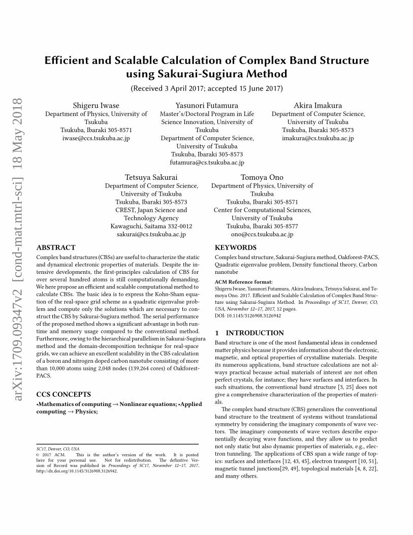
Figure 1: Relationship between the CBS and solutions of

QEP. Physically important eigenvalues within the green

shaded area and the others are plotted asfilled blue and open

red dots, respectively.

Hamiltonian, the KS equation (1) in n th unit cell of crystalline

material can be rewrien as

− Hn,n−1 |ψn−1〉 + (E − Hn,n) |ψn〉 − Hn,n+1 |ψn+1〉 = 0, (2)

where |ψn〉 is the eigenstate of n th unit cell and Hi, j is the KS

Hamiltonian matrix between the i th and j th unit cell. In bulk,

Hn−1,n = H†n,n+1. e Bloch’s theorem yields following equations

for eigenstates,

|ψn+l 〉 = λl |ψn〉 , l = −1, 0, 1, (3)

where λ = e ika (a is the length of unit cell). By substituting (3) into

KS equation (2), one can obtain a QEP for λ from λ−1 to λ,

[−λ−1Hn,n−1 + (E − Hn,n) − λHn,n+1] |ψn〉 = 0. (4)

e dispersion of complex k values obtained by scanning the

energy E is known as the CBS. e states |λ | = 1 correspond to

propagating modes. e remaining states, |λ | , 1, decaying or

growing exponentially in real space, correspond to the evanescent

modes. Evanescent modes with too small or large |λ | are decaying

or growing so rapid that they contribute marginally on the physi-

cal phenomena. us, it is enough to calculate the only eigenpairs

of QEP (4) satisfying

λmin < |λ | < λ−1min, (5)

where the order of 0.1 is enough for λmin to obtain the CBS. To

find the target eigenvalues (5) efficiently, we employ the Sakurai-

Sugiura method which will be explained in the next section.

3 SAKURAI-SUGIURAMETHOD

Complex moment-based eigensolvers, proposed by Sakurai and

Sugiura [42] in 2003, compute all eigenvalues within the target

region using a contour integral. Regarding parallel computing ef-

ficiency, complex moment-based eigensolvers have a big advan-

tage compared with Krylov-type methods because the most time-

consuming part of the complex moment-based eigensolvers is the

contour integral, which is suitable for parallel computing rather

than the sequential procedure of the Krylov-type methods. Based

on the contour integral, the complex moment-based eigensolvers

have higher level hierarchical parallelism than others. anks to

this high-level hierarchical parallelism, complexmoment-based eigen-

solvers achieve higher scalability [24, 52].

Today, there are several complex moment-based eigensolvers

including direct extensions of the Sakurai-Sugiura’s approach [16–

19, 21] and FEAST eigensolver [38] and its variants [44, 53, 54]. For

details, we refer [20] and reference therein. e Sakurai-Sugiura

methods have been developed to nonlinear eigenvalue problems,

unlike the FEAST eigensolver. erefore, in this paper, we use the

Sakurai-Sugiura method using Hankel matrices [2] for solving the

target QEP (4).

In this section, we present the basic algorithm of the Sakurai-

Sugiuramethod. We also introduce an improvement technique and

a parallel implementation of the Sakurai-Sugiura method special-

ized for the target QEP (4).

3.1 Basic algorithm of Sakurai-Sugiura method

Let Nrh ,Nmm ∈ N be input parameters and V ∈ CN×Nrh be an

input matrix. We define complex moment matrices

Sk :=1

2π i

∮

Γ

zkP(z)−1V dz, (6)

where

P(λ) = −λ−1Hn,n−1 + (E − Hn,n) − λHn,n+1.

eSakurai-Sugiuramethod and other complexmoment-based eigen-

solvers are mathematically designed based on the properties of the

complex moment matrices Sk . en, practical algorithms are de-

rived by approximating the contour integral (6) using Nint points

of numerical integration rule:

Sk :=

Nint∑

j=1

ωjzkj P(z j )

−1V (7)

where z j is a quadrature point on the boundary Γ of the target

region Ω and ωj is its corresponding weight. e practical algo-

rithms comprise the following three steps:

Step 1. Solve Nint linear systems with Nrh right-hand sides:

P(z j )Yj = V , j = 1, 2, . . . ,Nint . (8)

Step 2. Construct complexmomentmatrices, Sk and/or others, from

Yj (j = 1, 2, . . . ,Nint ).

Step 3. Extract the target (approximate) eigenpairs from the com-

plex moment matrices.

e Sakurai-Sugiura method [2] defines complex moment ma-

trices µk = V†Sk and extracts the target (approximate) eigenpairs

by solving Nrh × Nmm ≪ N dimensional generalized eigenvalue

problem with block Hankel matrices

[T <]i j = µi+j−1, [T ]i j = µi+j−2, 1 ≤ i, j ≤ Nmm .

To reduce the computational costs and improve the numerical

stability, we usually introduce a low-rank approximation with a

numerical rank m of T based on singular value decomposition:

T = [U1,U2]

[Σ1 O

O Σ2

] [W

†1

W†2

]≈ U1Σ1W

†1 .

SC17, November 12–17, 2017, Denver, CO, USA S. Iwase et al.

Algorithm 1 Sakurai-Sugiura method for QEP

Input: Nrh ,Nmm ,Nint ∈ N,δ ∈ R,V ∈ CN×Nrh , (z j ,ωj ) for j =

1, 2, . . . ,NintOutput: m approximate eigenpairs (λ, |ψn〉)

1: Compute Sk =∑Nint

j=1 ωjzkj P(z j )

−1V and µk = V†Sk

2: Set S = [S0, S1, . . . , SNmm−1] and block Hankel matrices T <, T

3: Compute a low-rank approximation of T using the threshold

δ : T = [U1,U2][Σ1,O ;O, Σ2][W1,W2]† ≈ U1Σ1W

†1

4: Solve U †1 T

<W1Σ−11 |ϕ〉 = τ |ϕ〉,

and compute (λ, |ψn〉) = (τ , SW1Σ−11 |ϕ〉)

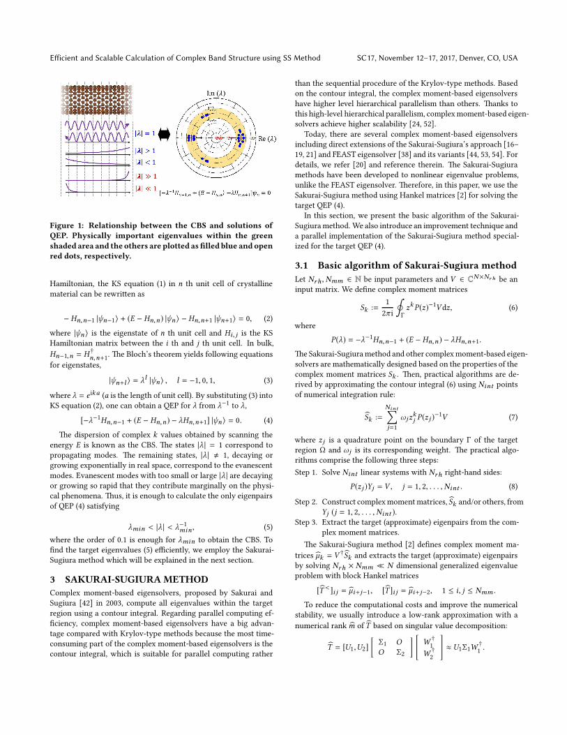
Figure 2: Contour path for the target ring-shaped region.

e target eigenvalues and the others are shown by • and

, respectively.

As a result, the target QEP (4) is reduced to an m dimensional stan-

dard eigenvalue problem, i.e.,

U†1 T

<W1Σ−11 |ϕ〉 = τ |ϕ〉 .

e (approximate) eigenpairs are obtained as (λ, |ψn〉) = (τ , SW1Σ−11 |ϕ〉),

where S = [S0, S1, . . . , SNmm−1]. e algorithm of the Sakurai-

Sugiura method is summarized in Algorithm 1.

3.2 Improvement technique using the specialstructure of the target QEP

e target eigenvalues (5) are located in a ring-shaped region be-

tween two circles with center at the origin. Radius of the small

and large circles are λmin and λ−1min , respectively. In this case, the

contour path is set as shown in Figure 2 and the complex moment

matrix Sk (6) is defined by

Sk :=1

2π i

∮

Γ1

zkP(z)−1V dz −1

2π i

∮

Γ2

zkP(z)−1V dz;

see [30].

Here, we let Nint as the number of quadrature points for each

circle. en, the complex moment Sk (7) is computed by

Sk =

Nint∑

j=1

ωj (z(1)j )kP(z

(1)j )−1V −

Nint∑

j=1

ωj (z(2)j )kP(z

(2)j )−1V ,

where the quadrature points are

z(1)j = λ

−1min exp(iθj ), z

(2)j = λmin exp(iθj )

and their corresponding weights are

ωj =1

Nintexp(iθj ),

with θj = 2π (j−1/2)/Nint . e number of linear systems we need

to solve is 2 × Nint , i.e.,

P(z(1)j )Y

(1)j = V , (9)

P(z(2)j )Y

(2)j = V , (10)

for j = 1, 2, . . . ,Nint , because the target region consists of two

circles, Γ1, Γ2.

e computational costs for solving the linear systems (9) and

(10) can be reduced to half using the special structure of the target

QEP (4). Because Hn,n−1 = H†n,n+1 and (E − Hn,n) = (E − Hn,n)

†,

we have

P(λ)† = P(1/λ).

erefore, the linear systems (10) is replaced as the dual systems

of (9), i.e.,

P(z(1)j )†Y

(2)j = V , (11)

because z(2)j = 1/z

(1)j .

Some linear solvers including (sparse) direct solvers and the bi-

conjugate gradient (BiCG) method efficiently solve the linear sys-

tems (9) and its dual systems (11) [41]. Specifically, the BiCGmethod

can solve both systems with almost the same costs for solving only

(9). erefore, in this paper, we select the BiCG method for solving

linear systems in the Sakurai-Sugiura method.

3.3 Parallel implementation for the target QEP

e most time-consuming part of the Sakurai-Sugiura method for

solving QEP (4) is Step 1 that is solving Nint linear systems with

Nrh right-hand sides (9) and their dual systems (11). For this part,

we use three layers of hierarchical parallelismof the Sakurai-Sugiura

method (Figure 3).

• Top layer: Multiple right-hand sides

As the linear systems (9) and (11) have Nrh right-hand

sides, we can independently solve these linear systems in

Nrh parallel without communication.

is parallelism requires no communication. Also, it is

expected to have good load balancing because the conver-

gence of the BiCG method does not strongly depend on

right-hand sides.

• Middle layer: adrature points

As the linear systems (9) and (11) are independent of j

(index of quadrature point), we can independently solve

these linear systems in Nint parallel without communica-

tion.

is parallelism requires no communication; however,

we need to take care of load balancing due to the imbal-

ance of the convergence of the BiCG method. To achieve

good load balancing, we use the following two stopping

conditions for the BiCG method.

Efficient and Scalable Calculation of Complex Band Structure using SS Method SC17, November 12–17, 2017, Denver, CO, USA

Figure 3: Hierarchical parallelism of the Sakurai-Sugiura

method.

– Relative residual 2-norm becomes less than certain

stopping criteria. (is is a standard stopping condi-

tion.)

– e BiCG method is stopped at over half of quadra-

ture points. (is is used to achieve good load balanc-

ing.)

• Bottom layer: Each linear system

e BiCG method is parallelized using domain decompo-

sition for solving each linear system.

is parallelism based on the domain decomposition

requires communication in matrix-vector multiplications

and inner products.

e total parallelism Ntotal is

Ntotal = Ndm × Nint × Nrh ,

where Ndm is the number of processors assigned for the domain

decomposition. If the number of processors we can use is less than

Nint ×Nrh , we use top layer parallelism first, because upper layer

is expected to show beer scalability than lower layers.

4 PERFORMANCE TEST

In this section, we present a series of test calculations of the CBS.

e KS Hamiltonian in the KS equation (1) is obtained from the

electronic structure calculations using the real-space DFT code,

RSPACE [14, 33]. All calculations in this section and later are per-

formed using the norm-conserving pseudopotential proposed by

Troullier and Martins [47]. e exchange-correlation interaction

is treated by the local density approximation (LDA) [37] and nine-

point finite-difference approximation is used for the Laplacian op-

erator. In every case we only use the Γ point sampling in the two-

dimensional Brillouin zone and typically set a grid spacing of 0.2

angstrom.

4.1 Serial performance

Weexperimentally evaluated the serial performance of ourmethod.

Here, we considered bulk Al(100) and (6,6) armchair CNTs with 4

and 24 atoms per unit cell, respectively. e number of grid points,

Nx ×Ny ×Nz , were 20× 20× 20 and 72× 72× 12, respectively. e

z-axis was parallel to the 〈100〉 direction (the nanotube axis) in the

case of the bulk Al(100) (CNT). We set Nint = 32,Nmm = 8,Nrh =

16,δ = 10−10 and λmin = 0.5. e convergence criteria of the

BiCG method was set to 10−10. All calculations described in this

subsection were carried out on a two-socket Intel Xeon E5-2683v4

with 16 cores (2.1 GHz) and 128 GB of system memory. We used

the Intel Fortran compiler and Intel Math Kernel Library (MKL).

To demonstrate excellent performance of the proposed method,

the computational cost was compared with that of the overbridg-

ing boundary matching (OBM) method [11], which is categorized

as a transfer-matrix method and is the best known algorithm of the

real-space grid approach. Although several improvements were

proposed aer the first study of the OBMmethod [32, 34], they did

not eliminate the computations of the first and last Nx × Ny × Nf

columns of (E − Hn,n)−1 and the generalized eigenvalue problem

for the 2×Nx×Ny×Nf dimensional matrices, whereNf is the order

of the finite-difference approximation [7]. In this study, the inver-

sion matrix was calculated using the CG method, and the general-

ized eigenvalue problem was solved using the optimized LAPACK

routine, ZGGEV.

Figure 4(a) illustrates the runtimes of the CBS calculations at

E = EF , where EF is the Fermi energy. In both examples, we can

see that our method is surprisingly fast compared with the OBM

method. We note that the solutions within λmin < |λ | < λ−1minobtained by our method correspond to the OBM solutions. Com-

pared with the runtimes for Al(100), the speed-up is more promi-

nent for (6,6) CNT. is can be seen by looking at the difference

in computational complexity between the two methods. e OBM

method using ZGGEV has O(N 3) complexity, where N is the size

of the KS Hamiltonian, while our method typically has the O(N 2)

complexity of the Krylov subspace method until the subspace di-

agonalization in the Sakurai-Sugiura method becomes dominant.

Figure 5 shows the histories of the residual norms of the solution

vectors for linear equations at different z j . In both graphs, we can

see the trend that convergence does not strongly depend on the

choice of z j . When the half of the residual norms achieved 10−10,

that with the slowest convergence became less than 10−8. is

uniform convergence behavior of the residual norms guarantees

the accuracy of the present method when two stopping criteria for

quadrature points as mentioned in subsection 3.3 are used. In ad-

dition, the number of iterations which need to converge generally

increase as most O(N ) as the size of the KS Hamiltonian matrix

SC17, November 12–17, 2017, Denver, CO, USA S. Iwase et al.

becomes large. Actually, we can also see that the convergence of

(6,6) CNT is approximately twice as slow as that of Al(100), while

the matrix size for the (6,6) CNT is 7.8 times larger than that of the

Al(100). Because of the sparse matrix vector operations withO(N )

complexity, the BiCG procedure in our method scales to less than

O(N 2) complexity. A huge improvement is also made on the mem-

ory requirements: a factor of 33 and 604 for Al(100) and (6,6) CNT,

respectively, as shown in Figure 4(b). Clearly, this improvement

can be aributed to the fact that the OBMmethod treats dense ma-

triceswithO(N 2)memory complexity, while ourmethod treats the

sparse Hamiltonian matrix with O(N ) memory complexity. us,

our method is faster and more memory efficient.

Next, we evaluated the accuracy of our method. Ploing the

calculated complex k values which satisfy |λ | = 1 as a function

of the real energy E allows us to compare with the conventional

band structure obtained from the electric structure calculations. As

shown in Figure 6, the real k values (black dots) obtained by our

method are in good agreement with the conventional band struc-

tures (red curves), with an accuracy of 10−5. Moreover, ourmethod

is suitable for parallel computing, as described in the next section.

0

50

100

150

0.191GB

115.331GB

OBM QEP/SS

Mem

ory

(GB

)

(6,6)CNT

Memory usage

0

200000

400000

600000

115.379 h

0.085 h

OBM QEP/SS(6,6)CNT

solve eigenvalue problem

matrix inversion

0

80

160

240 solve eigenvalue problem

matrix inversion

143.891 s

11.345 s

OBM QEP/SS

Runti

me

(sec

.)

Al(100)

Runti

me

(sec

.)

0.0

0.3

0.6

0.9 Memory usage

703.173 MB

21.333 MB

OBM QEP/SS

Mem

ory

(GB

)

Al(100)

(a) Runtime

(b) Memory usage

Figure 4: Serial performance of the proposed (QEP/Sakurai-

Sugiura) and conventional (OBM) method.

Table 1: Breakdown of computational cost of the proposed

method

Al(100) (6,6) CNT

read matrix data [sec.] 0.104 0.209

solve linear equations [sec.] 11.207 304.884

extract eigenpairs [sec.] 0.138 0.831

Figure 5: Convergence behavior of the BiCG algorithm for

(a) Al(100) and (b) (6,6) CNT at E = EF . e figures show the

residual norms as functions of the number of iterations at

each integration point z j .

4.2 Parallel performance

e computational cost of the Sakurai-Sugiura method mainly de-

pends on the part that solves the linear equations (8), as shown

in Table 1. Consequently, to evaluate the parallel performance of

our method, we parallelized only this part of our code by using

OpenMP directives and the Intel Message Passing Interface (MPI)

library. As mentioned in the previous section, the three layers of

hierarchical parallelism of the Sakurai-Sugiura method, i.e., paral-

lelisms for multiple right-hand sides (top layer), quadratic points

(middle layer), and the domain decomposition (boom layer) were

introduced.

All calculations in this subsectionwere performed onOakforest-

PACS. Each computation node is an Intel Xeon PhiTM 7250 (code

Efficient and Scalable Calculation of Complex Band Structure using SS Method SC17, November 12–17, 2017, Denver, CO, USA

Figure 6: Complex band structure for (a) Al(100) and (b) (6,6)

CNT.e black dots indicate the numerical results obtained

by the proposed method. e red curves show the conven-

tionally calculated band structures for comparison.

name: Knights Landing); each node has 68 cores (1.4 GHz) and 96

GB of system memory. We here conducted numerical experiments

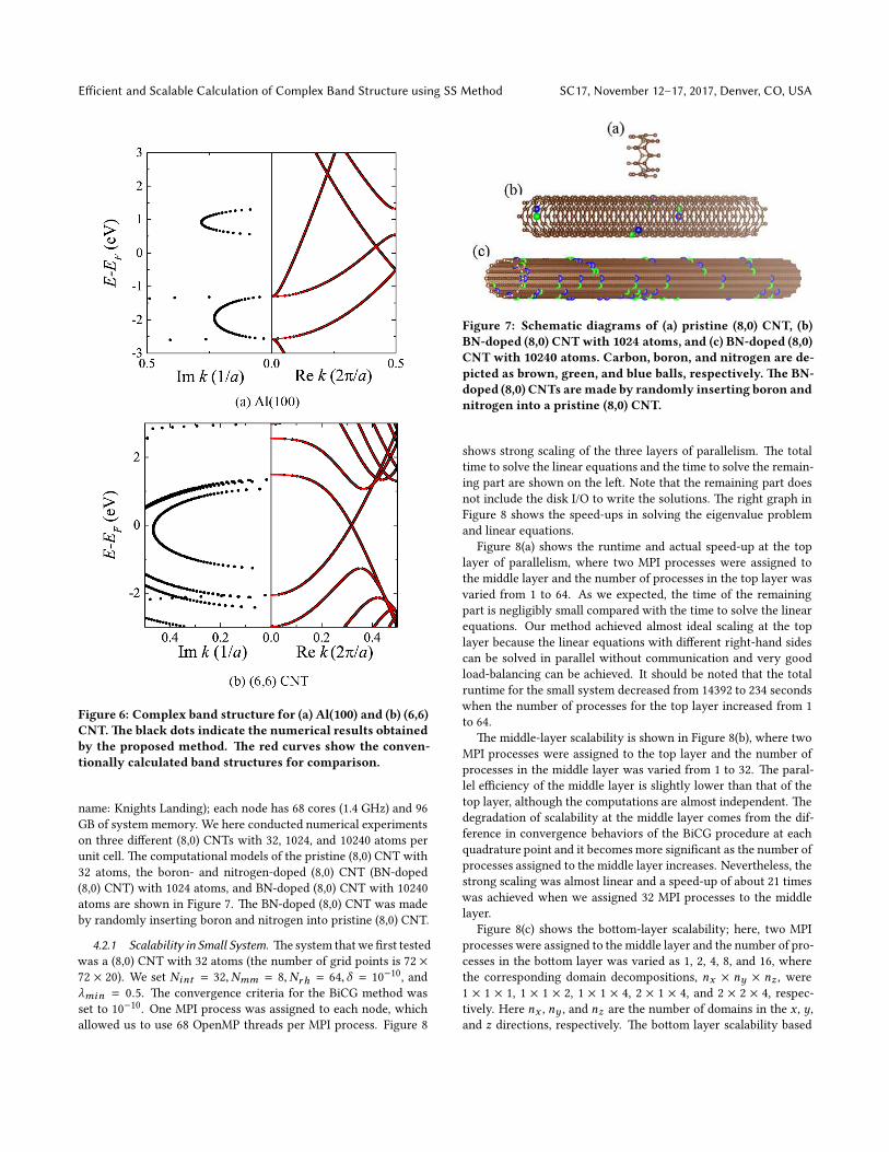
on three different (8,0) CNTs with 32, 1024, and 10240 atoms per

unit cell. e computational models of the pristine (8,0) CNT with

32 atoms, the boron- and nitrogen-doped (8,0) CNT (BN-doped

(8,0) CNT) with 1024 atoms, and BN-doped (8,0) CNT with 10240

atoms are shown in Figure 7. e BN-doped (8,0) CNT was made

by randomly inserting boron and nitrogen into pristine (8,0) CNT.

4.2.1 Scalability in Small System. esystem thatwe first tested

was a (8,0) CNT with 32 atoms (the number of grid points is 72 ×

72 × 20). We set Nint = 32,Nmm = 8,Nrh = 64,δ = 10−10, and

λmin = 0.5. e convergence criteria for the BiCG method was

set to 10−10. One MPI process was assigned to each node, which

allowed us to use 68 OpenMP threads per MPI process. Figure 8

Figure 7: Schematic diagrams of (a) pristine (8,0) CNT, (b)

BN-doped (8,0) CNT with 1024 atoms, and (c) BN-doped (8,0)

CNT with 10240 atoms. Carbon, boron, and nitrogen are de-

picted as brown, green, and blue balls, respectively. e BN-

doped (8,0) CNTs aremade by randomly inserting boron and

nitrogen into a pristine (8,0) CNT.

shows strong scaling of the three layers of parallelism. e total

time to solve the linear equations and the time to solve the remain-

ing part are shown on the le. Note that the remaining part does

not include the disk I/O to write the solutions. e right graph in

Figure 8 shows the speed-ups in solving the eigenvalue problem

and linear equations.

Figure 8(a) shows the runtime and actual speed-up at the top

layer of parallelism, where two MPI processes were assigned to

the middle layer and the number of processes in the top layer was

varied from 1 to 64. As we expected, the time of the remaining

part is negligibly small compared with the time to solve the linear

equations. Our method achieved almost ideal scaling at the top

layer because the linear equations with different right-hand sides

can be solved in parallel without communication and very good

load-balancing can be achieved. It should be noted that the total

runtime for the small system decreased from 14392 to 234 seconds

when the number of processes for the top layer increased from 1

to 64.

e middle-layer scalability is shown in Figure 8(b), where two

MPI processes were assigned to the top layer and the number of

processes in the middle layer was varied from 1 to 32. e paral-

lel efficiency of the middle layer is slightly lower than that of the

top layer, although the computations are almost independent. e

degradation of scalability at the middle layer comes from the dif-

ference in convergence behaviors of the BiCG procedure at each

quadrature point and it becomesmore significant as the number of

processes assigned to the middle layer increases. Nevertheless, the

strong scaling was almost linear and a speed-up of about 21 times

was achieved when we assigned 32 MPI processes to the middle

layer.

Figure 8(c) shows the boom-layer scalability; here, two MPI

processes were assigned to the middle layer and the number of pro-

cesses in the boom layer was varied as 1, 2, 4, 8, and 16, where

the corresponding domain decompositions, nx × ny × nz , were

1 × 1 × 1, 1 × 1 × 2, 1 × 1 × 4, 2 × 1 × 4, and 2 × 2 × 4, respec-

tively. Here nx , ny , and nz are the number of domains in the x , y,

and z directions, respectively. e boom layer scalability based

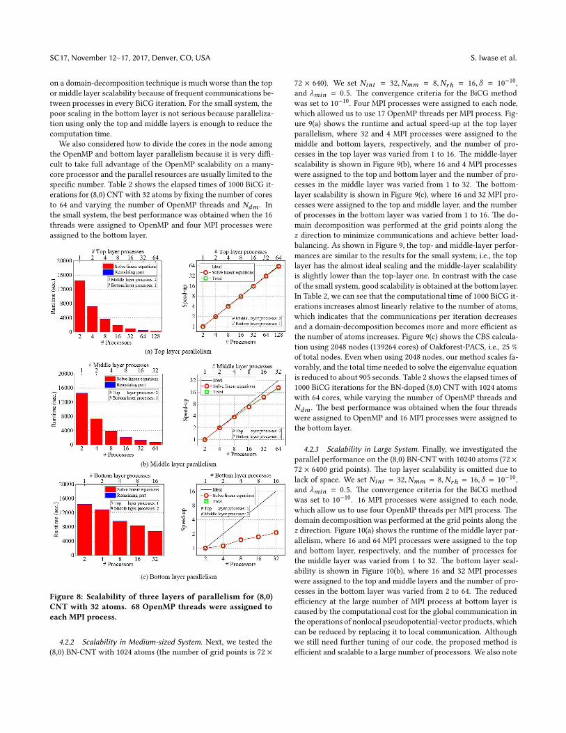
SC17, November 12–17, 2017, Denver, CO, USA S. Iwase et al.

on a domain-decomposition technique is much worse than the top

or middle layer scalability because of frequent communications be-

tween processes in every BiCG iteration. For the small system, the

poor scaling in the boom layer is not serious because paralleliza-

tion using only the top and middle layers is enough to reduce the

computation time.

We also considered how to divide the cores in the node among

the OpenMP and boom layer parallelism because it is very diffi-

cult to take full advantage of the OpenMP scalability on a many-

core processor and the parallel resources are usually limited to the

specific number. Table 2 shows the elapsed times of 1000 BiCG it-

erations for (8,0) CNT with 32 atoms by fixing the number of cores

to 64 and varying the number of OpenMP threads and Ndm . In

the small system, the best performance was obtained when the 16

threads were assigned to OpenMP and four MPI processes were

assigned to the boom layer.

Figure 8: Scalability of three layers of parallelism for (8,0)

CNT with 32 atoms. 68 OpenMP threads were assigned to

each MPI process.

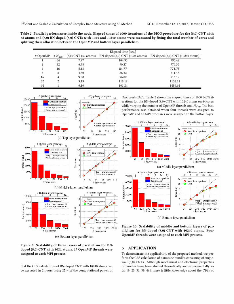
4.2.2 Scalability in Medium-sized System. Next, we tested the

(8,0) BN-CNT with 1024 atoms (the number of grid points is 72 ×

72 × 640). We set Nint = 32,Nmm = 8,Nrh = 16,δ = 10−10,

and λmin = 0.5. e convergence criteria for the BiCG method

was set to 10−10. Four MPI processes were assigned to each node,

which allowed us to use 17 OpenMP threads per MPI process. Fig-

ure 9(a) shows the runtime and actual speed-up at the top layer

parallelism, where 32 and 4 MPI processes were assigned to the

middle and boom layers, respectively, and the number of pro-

cesses in the top layer was varied from 1 to 16. e middle-layer

scalability is shown in Figure 9(b), where 16 and 4 MPI processes

were assigned to the top and boom layer and the number of pro-

cesses in the middle layer was varied from 1 to 32. e boom-

layer scalability is shown in Figure 9(c), where 16 and 32 MPI pro-

cesses were assigned to the top and middle layer, and the number

of processes in the boom layer was varied from 1 to 16. e do-

main decomposition was performed at the grid points along the

z direction to minimize communications and achieve beer load-

balancing. As shown in Figure 9, the top- and middle-layer perfor-

mances are similar to the results for the small system; i.e., the top

layer has the almost ideal scaling and the middle-layer scalability

is slightly lower than the top-layer one. In contrast with the case

of the small system, good scalability is obtained at the boom layer.

In Table 2, we can see that the computational time of 1000 BiCG it-

erations increases almost linearly relative to the number of atoms,

which indicates that the communications per iteration decreases

and a domain-decomposition becomes more and more efficient as

the number of atoms increases. Figure 9(c) shows the CBS calcula-

tion using 2048 nodes (139264 cores) of Oakforest-PACS, i.e., 25 %

of total nodes. Even when using 2048 nodes, our method scales fa-

vorably, and the total time needed to solve the eigenvalue equation

is reduced to about 905 seconds. Table 2 shows the elapsed times of

1000 BiCG iterations for the BN-doped (8,0) CNT with 1024 atoms

with 64 cores, while varying the number of OpenMP threads and

Ndm . e best performance was obtained when the four threads

were assigned to OpenMP and 16 MPI processes were assigned to

the boom layer.

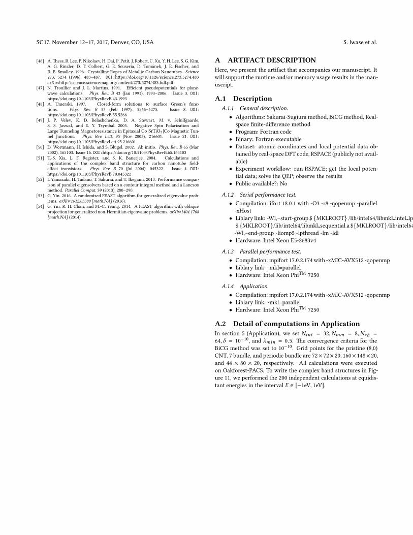
4.2.3 Scalability in Large System. Finally, we investigated the

parallel performance on the (8,0) BN-CNT with 10240 atoms (72×

72 × 6400 grid points). e top layer scalability is omied due to

lack of space. We set Nint = 32,Nmm = 8,Nrh = 16,δ = 10−10,

and λmin = 0.5. e convergence criteria for the BiCG method

was set to 10−10. 16 MPI processes were assigned to each node,

which allow us to use four OpenMP threads per MPI process. e

domain decomposition was performed at the grid points along the

z direction. Figure 10(a) shows the runtime of the middle layer par-

allelism, where 16 and 64 MPI processes were assigned to the top

and boom layer, respectively, and the number of processes for

the middle layer was varied from 1 to 32. e boom layer scal-

ability is shown in Figure 10(b), where 16 and 32 MPI processes

were assigned to the top and middle layers and the number of pro-

cesses in the boom layer was varied from 2 to 64. e reduced

efficiency at the large number of MPI process at boom layer is

caused by the computational cost for the global communication in

the operations of nonlocal pseudopotential-vector products, which

can be reduced by replacing it to local communication. Although

we still need further tuning of our code, the proposed method is

efficient and scalable to a large number of processors. We also note

Efficient and Scalable Calculation of Complex Band Structure using SS Method SC17, November 12–17, 2017, Denver, CO, USA

Table 2: Parallel performance inside the node. Elapsed times of 1000 iterations of the BiCG procedure for the (8,0) CNT with

32 atoms and (8,0) BN-doped (8,0) CNTs with 1024 and 10240 atoms were measured by fixing the total number of cores and

splitting their allocation between the OpenMP and bottom layer parallelism.

Elapsed time [sec.]

# OpenMP # Ndm (8,0) CNT (32 atoms) BN-doped (8,0) CNT (1024 atoms) BN-doped (8,0) CNT (10240 atoms)

1 64 7.77 104.95 795.42

2 32 6.78 90.37 776.35

4 16 5.18 84.77 774.75

8 8 4.50 86.32 811.43

16 4 3.98 96.02 916.12

32 2 5.19 118.12 1132.11

64 1 6.16 161.24 1486.64

Figure 9: Scalability of three layers of parallelism for BN-

doped (8,0) CNT with 1024 atoms. 17 OpenMP threads were

assigned to each MPI process.

that the CBS calculations of BN-doped CNT with 10240 atoms can

be executed in 2 hours using 25 % of the computational power of

Oakforest-PACS. Table 2 shows the elapsed times of 1000 BiCG it-

erations for the BN-doped (8,0) CNT with 10240 atoms on 64 cores

while varying the number of OpenMP threads and Ndm . e best

performance was obtained when four threads were assigned to

OpenMP and 16 MPI processes were assigned to the boom layer.

Figure 10: Scalability of middle and bottom layers of par-

allelism for BN-doped (8,0) CNT with 10240 atoms. Four

OpenMP threads were assigned to each MPI process.

5 APPLICATION

To demonstrate the applicability of the proposed method, we per-

form the CBS calculation of nanotube bundles consisting of single-

wall (8,0) CNTs. Although mechanical and electronic properties

of bundles have been studied theoretically and experimentally so

far [9, 23, 31, 39, 46], there is lile knowledge about the CBSs of

SC17, November 12–17, 2017, Denver, CO, USA S. Iwase et al.

Figure 11: Atomic structures and CBSs of (a) (8,0) CNT, (b) 7 bundle, and (c) crystalline bundle. Red dot in (a) denotes the

branch point. Carbon atoms are brown balls. In (c), the broken line represents the boundary of unit cell for crystalline bundle.

bundles. As far as we know, no aempt has been made. Up to now,

calculations of the CBS for carbon nano-materials have been lim-

ited within the empirical tight-binding approximation [27, 36, 51].

While the tight-binding approximation has been oen used suc-

cessfully for CNTs, it tends to reproduce the CBSs very poorly

when a CNT comes to interact with other CNTs. Figure 11 shows

the CBS of the isolated (8,0) CNT, seven, and crystalline bundles

with 32, 234, and 64 atoms, respectively. Due to the strong inter-

tube interaction, the band dispersions of bundles are enhanced and

the insulator-metal transition is occurred at crystalline bundles. As

for imaginary k region, the loop curvatures around the Fermi en-

ergy are enlarged by bundling, and the branch point in isolated

(8,0) CNT is kicked out from the band gap, which cannot be ex-

pected by conventional band structures.

For the calculation of the CBS for 7 bundle which is the largest

system in this section, it took about 1000 seconds for solving the

QEP at each E using the 512 nodes of Oakforest-PACS. is result

shows that first-principles CBS calculations for several hundred

atoms system can be performed as daily tasks using only a small

amount of the total resource of Oakforest-PACS.

6 CONCLUSION

We present an efficient and scalable method for the first-principles

calculation of CBS based on real-space grid approach. To take the

advantage of sparsity of the KS Hamiltonian in real-space, we di-

rectly solve a quadratic eigenvalue problem for a sparse matrix

by the Sakurai-Sugiura method to obtain the target eigenvalues

that correspond to the CBS, instead of computing the matrix in-

version and solving an eigenvalue problem for dense matrix. Ex-

perimental results on bulk Al(100) and (6,6) CNT show that the

proposed method outperforms the best known method [11] for

real-space grid approach by two orders of magnitude in both speed

and memory without sacrificing accuracy. Furthermore, owing to

the multiple layers of parallelism in the Sakurai-Sugiura method

and a domain-decomposition technique for real-space grids, the

proposed method scales very well to a large number of processors

and allows us to perform unprecedented simulations to investigate

the properties of material without translational symmetry. Using

2048 nodes (139264 cores) of Oakforest-PACS, we demonstrated

that the simulation of BN-doped (8,0) CNTs with 10240 atoms can

be executed in 2 hours. Extending the proposed method to other

formalisms which are computationally intractable by conventional

methods is one of the future directions.

ACKNOWLEDGMENTS

e authors would like to thank Y. Hirokawa and T. Boku for help-

ful discussion. is research was partially supported by MEXT as

a social and scientific priority issue (Creation of new functional de-

vices and high-performance materials to support next-generation

Efficient and Scalable Calculation of Complex Band Structure using SS Method SC17, November 12–17, 2017, Denver, CO, USA

industries) to be tackled by using post-K computer, and a Grant-

in-Aid for JSPS 221 Research Fellow (Grant No. 16J00911). is

work was supported in part by JST/CREST, JST/ACT-I (Grant No.

JP-MJPR16U6), and MEXT KAKENHI (Grant No. 17K12690). e

numerical calculations were carried out on the Oakforest-PACS of

Joint Center for Advanced High Performance Computing.

REFERENCES[1] Oakforest-PACS. hp://jcahpc.jp/eng/ofp intro.html[2] J. Asakura, T. Sakurai, H. Tadano, T. Ikegami, and K. Kimura. 2009. A numeri-

cal method for nonlinear eigenvalue problems using contour integrals. JSIAMLeers 1 (2009), 52–55. DOI:hps://doi.org/10.14495/jsiaml.1.52

[3] N. Ashcro and N. Mermin. 1976. Solid State Physics. Saunders College, Philadel-phia.

[4] J. Betancourt, S. Li, X. Dang, J. D. Burton, E. Y. Tsymbal, andJ. P. Velev. 2016. Complex band structure of topological insulator Bi2 Se 3. Journal of Physics: Condensed Maer 28, 39 (2016), 395501.hp://stacks.iop.org/0953-8984/28/i=39/a=395501

[5] Y.-C. Chang and J. N. Schulman. 1982. Complex band structures of crystallinesolids: An eigenvalue method. Phys. Rev. B 25 (Mar 1982), 3975–3986. Issue 6.DOI:hps://doi.org/10.1103/PhysRevB.25.3975

[6] J. R. Chelikowsky, N. Troullier, and Y. Saad. 1994. Finite-difference-pseudopotential method: Electronic structure calculations withouta basis. Phys. Rev. Le. 72 (Feb 1994), 1240–1243. Issue 8. DOI:

hps://doi.org/10.1103/PhysRevLe.72.1240[7] J. R. Chelikowsky, N. Troullier, K. Wu, and Y. Saad. 1994. Higher-

order finite-difference pseudopotential method: An application to diatomicmolecules. Phys. Rev. B 50 (Oct 1994), 11355–11364. Issue 16. DOI:

hps://doi.org/10.1103/PhysRevB.50.11355[8] X. Dang, J. D. Burton, A. Kalitsov, J. P. Velev, and E. Y. Tsymbal. 2014. Complex

band structure of topologically protected edge states. Phys. Rev. B 90 (Oct 2014),155307. Issue 15. DOI:hps://doi.org/10.1103/PhysRevB.90.155307

[9] H. Dumlich and S. Reich. 2011. Nanotube bundles and tube-tube orientation:A van der Waals density functional study. Phys. Rev. B 84 (Aug 2011), 064121.Issue 6. DOI:hps://doi.org/10.1103/PhysRevB.84.064121

[10] G. Fagas, A. Kambili, and M. Elstner. 2004. Complex-band struc-ture: a method to determine the off-resonant electron transport inoligomers. Chemical Physics Leers 389, 4-6 (2004), 268 – 273. DOI:

hps://doi.org/10.1016/j.cple.2004.03.090[11] Y. Fujimoto andK. Hirose. 2003. First-principles treatments of electron transport

properties for nanoscale junctions. Phys. Rev. B 67 (May 2003), 195315. Issue 19.DOI:hps://doi.org/10.1103/PhysRevB.67.195315

[12] V. Heine. 1964. Some theory about surface states. Surface Science 2 (1964), 1 – 7.DOI:hps://doi.org/10.1016/0039-6028(64)90036-6

[13] J. Heyd, G. E. Scuseria, and M. Ernzerhof. 2003. Hybrid function-als based on a screened Coulomb potential. e Journal of ChemicalPhysics 118, 18 (2003), 8207–8215. DOI:hps://doi.org/10.1063/1.1564060arXiv:hp://dx.doi.org/10.1063/1.1564060

[14] K. Hirose, T. Ono, Y. Fujimoto, and S. Tsukamoto. 2005. First-Principles Calcula-tions in Real-Space Formalism, Electronic Configurations and Transport Propertiesof Nanostructures. Imperial College Press, London.

[15] P. Hohenberg and W. Kohn. 1964. Inhomogeneous ElectronGas. Phys. Rev. 136 (Nov 1964), B864–B871. Issue 3B. DOI:

hps://doi.org/10.1103/PhysRev.136.B864[16] T. Ikegami and T. Sakurai. 2010. Contour integral eigensolver for non-Hermitian

systems: a Rayleigh-Ritz-type approach. Taiwan. J. Math. 14 (2010), 825–837.[17] T. Ikegami, T. Sakurai, and U. Nagashima. 2008. A filter diagonalization for

generalized eigenvalue problems based on the Sakurai-Sugiura projection method.Technical Report CS-TR-08-13. Department of Computer Science, University ofTsukuba.

[18] T. Ikegami, T. Sakurai, and U. Nagashima. 2010. A filter diagonalization for gen-eralized eigenvalue problems based on the Sakurai-Sugiura projection method.J. Comput. Appl. Math. 233 (2010), 1927–1936.

[19] A. Imakura, L. Du, and T. Sakurai. 2014. A block Arnoldi-type contour integralspectral projection method for solving generalized eigenvalue problems. Ap-plied Mathematics Leers 32 (2014), 22–27.

[20] A. Imakura, L. Du, and T. Sakurai. 2016. Relationships among contour integral-based methods for solving generalized eigenvalue problems. Jpn. J. Ind. Appl.Math. 33 (2016), 721–750.

[21] A. Imakura and T. Sakurai. 2017. Block Krylov-type complex moment-basedeigensolvers for solving generalized eigenvalue problems. Numer. Alg. (2017).(accepted).

[22] H. Ishida and D. Wortmann. 2016. Relationship between embedding-potential eigenvalues and topological invariants of time-reversal invariantband insulators. Phys. Rev. B 93 (Mar 2016), 115415. Issue 11. DOI:

hps://doi.org/10.1103/PhysRevB.93.115415[23] S. Kazaoui, N. Minami, H. Yamawaki, K. Aoki, H. Kataura, and Y. Achiba.

2000. Pressure dependence of the optical absorption spectra of single-walledcarbon nanotube films. Phys. Rev. B 62 (Jul 2000), 1643–1646. Issue 3. DOI:hps://doi.org/10.1103/PhysRevB.62.1643

[24] J. Kestyn, V. Kalantzis, E. Polizzi, and Y. Saad. 2016. PFEAST: a high performancesparse eigenvalue solver using distributed-memory linear solvers. In SC’16 pro-ceeding of the International Conference for High Performance Computing, Net-working, Storage and Analysis.

[25] C. Kiel. 1986. Introduction to Solid State Physics (6th ed.). John Wiley & Sons,Inc., New York.

[26] W. Kohn and L. J. Sham. 1965. Self-Consistent Equations Including Exchangeand Correlation Effects. Phys. Rev. 140 (Nov 1965), A1133–A1138. Issue 4A. DOI:hps://doi.org/10.1103/PhysRev.140.A1133

[27] D. H. Lee and J. D. Joannopoulos. 1981. Simple scheme for surface-bandcalculations. I. Phys. Rev. B 23 (May 1981), 4988–4996. Issue 10. DOI:hps://doi.org/10.1103/PhysRevB.23.4988

[28] M. Luisier, A. Schenk, W. Fichtner, and G. Klimeck. 2006. Atomistic simulation

of nanowires in the sp3d 5s∗ tight-binding formalism: From boundary condi-tions to strain calculations. Phys. Rev. B 74 (Nov 2006), 205323. Issue 20. DOI:hps://doi.org/10.1103/PhysRevB.74.205323

[29] P. Mavropoulos, N. Papanikolaou, and P. H. Dederichs. 2000. ComplexBand Structure and Tunneling through Ferromagnet /Insulator /FerromagnetJunctions. Phys. Rev. Le. 85 (Jul 2000), 1088–1091. Issue 5. DOI:

hps://doi.org/10.1103/PhysRevLe.85.1088[30] T. Miyata, L. Du, T. Sogabe, Y. Yamamoto, and S.-L. Zhang. 2009. An Extension

of the Sakurai-SugiuraMethod for Eigenvalue Problems of Multiply ConnectedRegion (in Japanese). Transactions of JSIAM 19 (2009), 537–550.

[31] S. Okada, A. Oshiyama, and S. Saito. 2001. Pressure and Orientation Effects onthe Electronic Structure of CarbonNanotube Bundles. Journal of the Physical So-ciety of Japan 70, 8 (2001), 2345–2352. DOI:hps://doi.org/10.1143/JPSJ.70.2345arXiv:hp://dx.doi.org/10.1143/JPSJ.70.2345

[32] T. Ono, Y. Egami, and K. Hirose. 2012. First-principles transport calcu-lation method based on real-space finite-difference nonequilibrium Green’sfunction scheme. Phys. Rev. B 86 (Nov 2012), 195406. Issue 19. DOI:

hps://doi.org/10.1103/PhysRevB.86.195406[33] T. Ono and K. Hirose. 1999. Timesaving Double-Grid Method for Real-Space

Electronic-Structure Calculations. Phys. Rev. Le. 82 (Jun 1999), 5016–5019. Is-sue 25. DOI:hps://doi.org/10.1103/PhysRevLe.82.5016

[34] T. Ono and S. Tsukamoto. 2016. Real-space method for first-principleselectron transport calculations: Self-energy terms of electrodes forlarge systems. Phys. Rev. B 93 (Jan 2016), 045421. Issue 4. DOI:

hps://doi.org/10.1103/PhysRevB.93.045421[35] J. Paier, M. Marsman, K. Hummer, G. Kresse, I. C. Gerber, and J. G. Angyan.

2006. Screened hybrid density functionals applied to solids. e Journal ofChemical Physics 124, 15 (2006), 154709. DOI:hps://doi.org/10.1063/1.2187006arXiv:hp://dx.doi.org/10.1063/1.2187006

[36] C. Park, J. Ihm, and G. Kim. 2013. Decay behavior of localized states at recon-structed armchair graphene edges. Phys. Rev. B 88 (Jul 2013), 045403. Issue 4.DOI:hps://doi.org/10.1103/PhysRevB.88.045403

[37] J. P. Perdew and A. Zunger. 1981. Self-interaction correction to density-functional approximations for many-electron systems. Phys. Rev. B 23 (May1981), 5048–5079. Issue 10. DOI:hps://doi.org/10.1103/PhysRevB.23.5048

[38] E. Polizzi. 2009. A density matrix-based algorithm for solving eigenvalue prob-lems. Phys. Rev. B 79 (2009), 115112.

[39] S. Reich, C.omsen, and P. Ordejon. 2002. Electronic band structure of isolatedand bundled carbon nanotubes. Phys. Rev. B 65 (Mar 2002), 155411. Issue 15. DOI:hps://doi.org/10.1103/PhysRevB.65.155411

[40] M. G. Reuter, T. Seideman, and M. A. Ratner. 2011. Probing the surface-to-bulk transition: A closed-form constant-scaling algorithm for computing sub-surface Green functions. Phys. Rev. B 83 (Feb 2011), 085412. Issue 8. DOI:hps://doi.org/10.1103/PhysRevB.83.085412

[41] Y. Saad. 2003. Iterative Methods for Sparse Linear Systems (2nd ed.). Society forIndustrial and Applied Mathematics, Philadelphia, PA, USA.

[42] T. Sakurai and H. Sugiura. 2003. A projection method for generalized eigenvalueproblems using numerical integration. J. Comput. Appl. Math. 159, 1 (2003), 119– 128. DOI:hps://doi.org/10.1016/S0377-0427(03)00565-X 6th Japan-ChinaJoint Seminar on Numerical Mathematics; In Search for the Frontier of Compu-tational and Applied Mathematics toward the 21st Century.

[43] J. N. Schulman and Y.-C. Chang. 1981. New method for calculating electronicproperties of superlaices using complex band structures. Phys. Rev. B 24 (Oct1981), 4445–4448. Issue 8. DOI:hps://doi.org/10.1103/PhysRevB.24.4445

[44] P. T. P. Tang and E. Polizzi. 2014. FEAST as a subspace iteration eigensolveraccelerated by approximate spectral projection. SIAM J. Matrix Anal. Appl. 35(2014), 354–390.

[45] J. Tersoff. 1984. eory of semiconductor heterojunctions: e role ofquantum dipoles. Phys. Rev. B 30 (Oct 1984), 4874–4877. Issue 8. DOI:hps://doi.org/10.1103/PhysRevB.30.4874

SC17, November 12–17, 2017, Denver, CO, USA S. Iwase et al.

[46] A.ess, R. Lee, P. Nikolaev, H. Dai, P. Petit, J. Robert, C. Xu, Y. H. Lee, S. G. Kim,A. G. Rinzler, D. T. Colbert, G. E. Scuseria, D. Tomanek, J. E. Fischer, andR. E. Smalley. 1996. Crystalline Ropes of Metallic Carbon Nanotubes. Science273, 5274 (1996), 483–487. DOI:hps://doi.org/10.1126/science.273.5274.483arXiv:hp://science.sciencemag.org/content/273/5274/483.full.pdf

[47] N. Troullier and J. L. Martins. 1991. Efficient pseudopotentials for plane-wave calculations. Phys. Rev. B 43 (Jan 1991), 1993–2006. Issue 3. DOI:hps://doi.org/10.1103/PhysRevB.43.1993

[48] A. Umerski. 1997. Closed-form solutions to surface Green’s func-tions. Phys. Rev. B 55 (Feb 1997), 5266–5275. Issue 8. DOI:

hps://doi.org/10.1103/PhysRevB.55.5266[49] J. P. Velev, K. D. Belashchenko, D. A. Stewart, M. v. Schilfgaarde,

S. S. Jaswal, and E. Y. Tsymbal. 2005. Negative Spin Polarization andLarge Tunneling Magnetoresistance in Epitaxial Co |SrTiO3 |Co Magnetic Tun-nel Junctions. Phys. Rev. Le. 95 (Nov 2005), 216601. Issue 21. DOI:

hps://doi.org/10.1103/PhysRevLe.95.216601[50] D. Wortmann, H. Ishida, and S. Blugel. 2002. Ab initio. Phys. Rev. B 65 (Mar

2002), 165103. Issue 16. DOI:hps://doi.org/10.1103/PhysRevB.65.165103[51] T.-S. Xia, L. F. Register, and S. K. Banerjee. 2004. Calculations and

applications of the complex band structure for carbon nanotube field-effect transistors. Phys. Rev. B 70 (Jul 2004), 045322. Issue 4. DOI:

hps://doi.org/10.1103/PhysRevB.70.045322[52] I. Yamazaki, H. Tadano, T. Sakurai, and T. Ikegami. 2013. Performance compar-

ison of parallel eigensolvers based on a contour integral method and a Lanczosmethod. Parallel Comput. 39 (2013), 280–290.

[53] G. Yin. 2016. A randomized FEAST algorithm for generalized eigenvalue prob-lems. arXiv:1612.03300 [math.NA] (2016).

[54] G. Yin, R. H. Chan, and M.-C. Yeung. 2014. A FEAST algorithm with obliqueprojection for generalized non-Hermitian eigenvalue problems. arXiv:1404.1768[math.NA] (2014).

A ARTIFACT DESCRIPTION

Here, we present the artifact that accompanies our manuscript. It

will support the runtime and/or memory usage results in the man-

uscript.

A.1 Description

A.1.1 General description.

• Algorithms: Sakurai-Sugiura method, BiCG method, Real-

space finite-difference method

• Program: Fortran code

• Binary: Fortran executable

• Dataset: atomic coordinates and local potential data ob-

tained by real-space DFT code, RSPACE (publicly not avail-

able)

• Experiment workflow: run RSPACE; get the local poten-

tial data; solve the QEP; observe the results

• Public available?: No

A.1.2 Serial performance test.

• Compilation: ifort 18.0.1 with -O3 -r8 -qopenmp -parallel

-xHost

• Liblary link: -Wl,–start-group $ MKLROOT /lib/intel64/libmkl intel lp64.a

$ MKLROOT/lib/intel64/libmkl sequential.a $MKLROOT/lib/intel64/libmkl core.a

-Wl,–end-group -liomp5 -lpthread -lm -ldl

• Hardware: Intel Xeon E5-2683v4

A.1.3 Parallel performance test.

• Compilation: mpifort 17.0.2.174with -xMIC-AVX512 -qopenmp

• Liblary link: -mkl=parallel

• Hardware: Intel Xeon PhiTM 7250

A.1.4 Application.

• Compilation: mpifort 17.0.2.174with -xMIC-AVX512 -qopenmp

• Liblary link: -mkl=parallel

• Hardware: Intel Xeon PhiTM 7250

A.2 Detail of computations in Application

In section 5 (Application), we set Nint = 32,Nmm = 8,Nrh =

64,δ = 10−10, and λmin = 0.5. e convergence criteria for the

BiCG method was set to 10−10. Grid points for the pristine (8,0)

CNT, 7 bundle, and periodic bundle are 72× 72× 20, 160× 148× 20,

and 44 × 80 × 20, respectively. All calculations were executed

on Oakforest-PACS. To write the complex band structures in Fig-

ure 11, we performed the 200 independent calculations at equidis-

tant energies in the interval E ∈ [−1eV, 1eV].