efficient antenna patterns for three- sector wcdma systemswcdma systems master of science thesis by...

Efficient Antenna Patterns for Three-Sector WCDMA Systems LI CHUNJIAN

Communication Systems Group Department of Signals and Systems Chalmers University of Technology Göteborg, Sweden, 2003 EX006/2003

Date Rev

No.Prepared (also subject responsible if other)

Approved Checked Reference

2003-02-06 A030206

ERA/TU-02:437

TUG

LI CHUNJIAN

1 (58)

EFFICIENT ANTENNA PATTERNS FOR THREE-SECTOR WCDMA SYSTEMS

MASTER OF SCIENCE THESIS

by Li Chunjian

Ericsson AB

Chalmers University of Technology

February, 2003

EX006/2003

Supervisors: Examiner:

Sven Petersson Professor Arne Svensson

Martin Johansson

Antenna Research Center, Signals and Systems Department,

Ericsson AB Chalmers University of Technology

Date Rev



2003-02-06 A030206

ERA/TU-02:437

TUG

LI CHUNJIAN

2 (58)

Abstract

This paper presents a comprehensive capacity study for the W-CDMA system, with focus on how the base station antenna radiation pattern affects system capacity in a sectorized system. Radiation patterns optimized with respect to highest capacity or lowest power consumption are found for a system with three-sector sites. The optimum beamwidth of commonly used single column antenna, whose radiation pattern is modeled by a cosine pattern, is also studied.

Date Rev



2003-02-06 A030206

ERA/TU-02:437

TUG

LI CHUNJIAN

3 (58)

Acknowledgement

I would like to express my gratitude to my supervisors Sven Petersson and Martin Johansson, both senior specialists at Antenna Research Center, Ericsson AB. During the project they had spend tremendous time discussing with me and reviewing my paper. I have learnt a lot more about W-CDMA system from Sven, and attained valuable knowledge about antenna system from Martin. I also learned in this project their precise scientific attitude to research work.

I would also like to thank the other colleagues in the center, for their support and sharing knowl-edge and their warm hospitality making me feel at home.

I am also grateful to professor Arne Svensson at Chalmers University of Technology, who lead me into the fascinating world of wireless communications and, as my examiner, provided me guidance in this work.

Finally, this thesis could not have been done without the great support from my wife, my parents, and my friends, you are the best thing in my life.

Date Rev



2003-02-06 A030206

ERA/TU-02:437

TUG

LI CHUNJIAN

4 (58)

Contents Page

1 Introduction. . . . . . . . . . . . . . . . . . . . . . . . . . . . . . . . . . . . . . . . . . . . . . . . . . . . 51.1 Background. . . . . . . . . . . . . . . . . . . . . . . . . . . . . . . . . . . . . . . . . . . . . . . . . . . . . 51.2 The structure . . . . . . . . . . . . . . . . . . . . . . . . . . . . . . . . . . . . . . . . . . . . . . . . . . . . 5

2 W-CDMA system downlink capacity analysis . . . . . . . . . . . . . . . . . . . . . . . . 72.1 Downlink power equation. . . . . . . . . . . . . . . . . . . . . . . . . . . . . . . . . . . . . . . . . . 7

2.1.1 Interference model . . . . . . . . . . . . . . . . . . . . . . . . . . . . . . . . . . . . . . . . . . . . . . . 72.1.2 Discrete user-distribution approach without handover . . . . . . . . . . . . . . . . . . . . 82.1.3 Continuous user-distribution approach without handover . . . . . . . . . . . . . . . . 102.1.4 Handover. . . . . . . . . . . . . . . . . . . . . . . . . . . . . . . . . . . . . . . . . . . . . . . . . . . . . . 10

2.2 Antenna model . . . . . . . . . . . . . . . . . . . . . . . . . . . . . . . . . . . . . . . . . . . . . . . . . 112.3 A comparison of approaches with discrete and continuous user distribution. . 12

3 Simulation setup . . . . . . . . . . . . . . . . . . . . . . . . . . . . . . . . . . . . . . . . . . . . . . . 134 Optimum piecewise-linear antenna pattern and system behavior study . 15

4.1 The optimization . . . . . . . . . . . . . . . . . . . . . . . . . . . . . . . . . . . . . . . . . . . . . . . . 154.2 The optimum pattern for maximum capacity . . . . . . . . . . . . . . . . . . . . . . . . . . 154.3 The optimum pattern for lowest base station output power at certain loads . . 174.4 Analysis to the optimization results . . . . . . . . . . . . . . . . . . . . . . . . . . . . . . . . . 184.5 About the system behavior . . . . . . . . . . . . . . . . . . . . . . . . . . . . . . . . . . . . . . . . 23

4.5.1 Non-unique optimum pattern . . . . . . . . . . . . . . . . . . . . . . . . . . . . . . . . . . . . . . 234.5.2 Cell range and capacity trade-off . . . . . . . . . . . . . . . . . . . . . . . . . . . . . . . . . . . 244.5.3 The diamond cell shape . . . . . . . . . . . . . . . . . . . . . . . . . . . . . . . . . . . . . . . . . . 254.5.4 Comparison of different site plans . . . . . . . . . . . . . . . . . . . . . . . . . . . . . . . . . . 264.5.5 Power control . . . . . . . . . . . . . . . . . . . . . . . . . . . . . . . . . . . . . . . . . . . . . . . . . . 274.5.6 Hand over . . . . . . . . . . . . . . . . . . . . . . . . . . . . . . . . . . . . . . . . . . . . . . . . . . . . . 29

5 Achieving maximum capacity with realistic antenna model . . . . . . . . . . . 336 Hand over and other issues . . . . . . . . . . . . . . . . . . . . . . . . . . . . . . . . . . . . . . 387 Uplink analysis . . . . . . . . . . . . . . . . . . . . . . . . . . . . . . . . . . . . . . . . . . . . . . . . 41

7.1 Uplink power equation . . . . . . . . . . . . . . . . . . . . . . . . . . . . . . . . . . . . . . . . . . . 417.2 Simulation results . . . . . . . . . . . . . . . . . . . . . . . . . . . . . . . . . . . . . . . . . . . . . . . 42

8 Comparison with previous study. . . . . . . . . . . . . . . . . . . . . . . . . . . . . . . . . . 449 Conclusion . . . . . . . . . . . . . . . . . . . . . . . . . . . . . . . . . . . . . . . . . . . . . . . . . . . . 4510 Future work. . . . . . . . . . . . . . . . . . . . . . . . . . . . . . . . . . . . . . . . . . . . . . . . . . . 46

References . . . . . . . . . . . . . . . . . . . . . . . . . . . . . . . . . . . . . . . . . . . . . . . . . . . . 47Terminology. . . . . . . . . . . . . . . . . . . . . . . . . . . . . . . . . . . . . . . . . . . . . . . . . . . 48

Appendix A : Downlink power equations . . . . . . . . . . . . . . . . . . . . . . . . . . . . . . . . . . . . . . . . . . . . . . . . . 49A.1 Discrete user-distribution approach without handover . . . . . . . . . . . . . . . . . . . 49A.2 Continuous user-distribution approach without handover . . . . . . . . . . . . . . . . 51A.3 Handover. . . . . . . . . . . . . . . . . . . . . . . . . . . . . . . . . . . . . . . . . . . . . . . . . . . . . . 52

Appendix B : The antenna model . . . . . . . . . . . . . . . . . . . . . . . . . . . . . . . . . . . . . . . . . . . . . . . . . . . . . . . . 54Appendix C : Simulation parameters . . . . . . . . . . . . . . . . . . . . . . . . . . . . . . . . . . . . . . . . . . . . . . . . . . . . . 55Appendix D: Uplink power equation . . . . . . . . . . . . . . . . . . . . . . . . . . . . . . . . . . . . . . . . . . . . . . . . . . . . . 57

Date Rev



2003-02-06 A030206

ERA/TU-02:437

TUG

LI CHUNJIAN

5 (58)

1 Introduction

This thesis presents an extensive capacity analysis for three-sector W-CDMA systems using an analytical approach and simulations based on downlink power equations. Antenna parameters and site plans are incorporated into the simulator so that they can be optimized for maximum capacity or lowest base station output power. Both non-realistic and realistic antenna models are used. An optimum azimuthal radiation pattern is found. Analysis of simulation results and con-clusions are made trying to reveal the whole system behavior, i.e. the relations between down-link power, system capacity, cell size, sectorization, antenna configuration, hand over, power control, and site plan. The optimized antenna parameters are justified and complemented by an uplink analysis.

1.1 Background

In order to make the envisioned mobile multi-media services possible, 3rd generation (3G) cel-lular systems are expected to provide at least two orders of magnitude higher data rates than the systems in operation at present. Combining this with other demanding factors, such as rapidly increasing number of subscribers (meaning higher density of users), limited radio bandwidth, harsher EMF restrictions and more focus on operation cost, the success of the 3rd generation mobile services will depend on highly efficient systems being organized in highly efficient ways. Techniques to improve performance from the aspects of system design and system de-ployment are under extensive research.

In a W-CDMA system, the active UEs are sources of interference to the system. As the number of active UEs increases, the system noise level is raised. This characteristic makes the system capacity and coverage closely related to each other. The interaction of traffic load and cell size, so called cell breathing, is one of the important factors when planning an efficient deployment of a W-CDMA network. There are typically two types of problems to solve. One is the coverage limited scenario: there is a small number of UEs to be served in a relatively large cell. What is the lowest output power required given a certain coverage area? Different antenna radiation pat-terns can produce quite different answers. The second is the capacity limited scenario: when there is a large number of UEs crowded in a small area, how many UEs can a cell serve at most? Again, antenna configuration and site plan affect the answer a lot.

In principle, from a system level point of view, the system spectrum efficiency and power effi-ciency (measured by the average power required to support a certain number of UEs) are linked to each other positively. The higher the power efficiency, the higher the spectrum efficiency. That means, if the system succeeds to lower the total transmitted power "in the air" (without loss of quality), it will be able to support more users with the same radio bandwidth. Thus it is very interesting to investigate the relation between signal power and MAI (multiple access interfer-ence), or capacity, to identify ways of optimizing system efficiency. An obvious choice of fac-tors that can be exploited for such optimization includes base station antenna parameters and site planning.

1.2 The structure

Since a W-CDMA system is designed to support high rate data services, which are typically of asymmetric traffic in nature, we follow the assumption that the downlink will carry higher data

Date Rev



2003-02-06 A030206

ERA/TU-02:437

TUG

LI CHUNJIAN

6 (58)

rate than the uplink and thus is the limiting factor in such a system. Consequently, in this study, the antenna parameters and other issues affecting downlink capacity will be in the focus, and then we also examine the uplink optimum as a complementary. Since the analysis of the optimi-zation result can be understood without reading the large volume of equation derivations, most of the equation derivations are given in the appendix.

Date Rev



2003-02-06 A030206

ERA/TU-02:437

TUG

LI CHUNJIAN

7 (58)

2 W-CDMA system downlink capacity analysis

Tremendous work have been done on the study of W-CDMA system capacity and there are many analytical expressions derived in literature. Most of them are derived from basic single cell interference expressions with an interference ratio (or the F-factor) to account for the inter-cell interference so that a multi-cell system is treated [1], [2], and [3]. To incorporate the antenna radiation pattern and a specific site plan, and to gain more insight into the whole system behav-ior, we use a more detailed multi-cell interference expression, a basic form of which was used previously in [4] to study optimum antenna parameters.

2.1 Downlink power equation

To avoid ambiguity, here we refer to the location of a base station providing coverage in a certain area as a site; every site is sectorized into three sectors by implementing directional base station antennas. A cell is defined to be the surface within which all UEs have their primary connection (the link with the best path gain) to the same base station sector antenna.

The analytical expression relating capacity (number of users) to the total output power of the base station is called downlink power equation here, which is essential to the study since it is the analytical basis of the simulations.

2.1.1 Interference model

The multi-cell interference model incorporating antenna radiation pattern is previously de-scribed in [5] and further developed in [6]. This model assumes an infinitely large site plan with an infinite number of cells, one of which is designated as the target cell. Each cell is occupied by identical sets of UEs (by distributing UEs randomly in the target cell and then reusing the same set of UE-locations for every cell). The site plan is assumed to be regular (the distance from site to site are identical). Thus any cell can be designated as target cell, because of the prop-erty of symmetry. Since all cells in this model possess exactly the same behavior, studying the target cell is sufficient to understand the whole system. As depicted in figure 1, the nominal cell shape is one third of a hexagon, and the target cell is chosen to be the one with the antenna point-ing towards the right. The actual cell shape is dependant of the basestation antenna radiation pat-tern, thus it is calculated individually for different antenna patterns. UEs in the target cell are distributed randomly with uniform probability over the area of the cell. Every cell in the system will have exactly the same UE distribution as in the target cell. By adding UEs into the cell until the total power limit per cell is exceeded, one can find out the capacity of the cell.

Date Rev



2003-02-06 A030206

ERA/TU-02:437

TUG

LI CHUNJIAN

8 (58)

Figure 1 The nominal cell shape, antenna directions, and UE distribution in the target cell.

Stochastic effects, such as fading, can be implicitly included in the model but will then affect all cells identically. Since we are primarily interested in the average behavior, we do not take shad-ow fading and fast fading into account. We assume that orthogonality within a cell is maintained regardless of the number of UEs, i.e., the available number of orthogonal codes is not the capac-ity-limiting factor. The system overhead, such as pilot, synchronization channel, etc., also con-sume downlink power, but it is low compared to the total power, especially when the system is fully loaded.

The downlink power equations are essential for evaluating the capacity. The derivations of these equations are described in detail in Appendix A. In the following sections only the result of the derivations are shown.

2.1.2 Discrete user-distribution approach without handover

Naturally, the number of UEs can only take an integer value. A certain number of UEs are ran-domly distributed in the target cell. The other cells serve the same number of UEs and their UE distributions are duplicates of that of the target cell. Given all the UE locations and the basesta-tion antenna radiation pattern, the path gain (the product of antenna gain, path loss and fading) between UEs and basestation antennas can be calculated. Thus we are able to calculate signal power and interference power seen by every UE and work out the equations relating SIR to downlink power. We assume the target SIR for every UE is identical in a uniform service sce-nario, thus the downlink power is a function of the number of UEs in the cell. By letting the total downlink power go to infinity we find the maximum number of UEs supported by a single cell. The equation for the maximum capacity is derived in Appendix A (equation A.7) and can be written as

Date Rev



2003-02-06 A030206

ERA/TU-02:437

TUG

LI CHUNJIAN

9 (58)

(1)

where Nu is the capacity (number of UEs per cell), is the orthogonality factor, C is the number of cells in the system, GP is the processing gain, SIR is the target signal-to-interference ratio, gc,n is the effective path gain for the signal path between antenna in cell c and UE number n in the target cell.

Because the users are discrete (the number of users can only be an integer) and randomly dis-tributed, only a single realization of UE-distribution will not tell the mean behavior of the sys-tem. One needs to evaluate the capacity based on a large number of UE-distributions and then take the average value.

It is obvious that to obtain a consistent mean system behavior one should solve the equation for maximum capacity with an infinite number of realizations of user distributions and average them. Due to limited computational resources we took only 100 realizations of user distributions and did the averaging. The plotting of the mean of the results of equation (1) vs. the number of realizations shows that the mean of the results tends to converge as the number of realizations increases, and after about 100 realizations it converges to within 1% difference of the mean val-ue. We consider this to be an acceptable approximation.

Figure 2 The mean of the result converges to within 1% difference of the mean value after 100 iterations

Nu1α---

gc n,g1 n,----------

GP

SIR----------–

c 1=

C

∑n 1=

Nu

∑ ⋅=

α

0 20 40 60 80 100 120 140 160 180 200

73

72.5

72

71.5

71

70.5

70

69.5

number of iterations

Cap

acity

(m

ax. n

o. o

f UE

s pe

r ce

ll)

Date Rev



2003-02-06 A030206

ERA/TU-02:437

TUG

LI CHUNJIAN

10 (58)

2.1.3 Continuous user-distribution approach without handover

We can avoid the deviation produced by averaging over a limited number of realizations, if we allow the number of UEs to be a continuous variable. The capacity is then expressed as a UE density over the cell area, which means that the first summation in equation (1) can be replaced by a surface integral, and Nu can now be written explicitly as

(2)

where A is the area of a cell, is the target cell, and gc(x,y) is the effective path gain for the signal path between the antenna in cell c and a position in the target cell given by the Cartesian coordinate pair (x, y). Since the UEs are assumed to be uniformly spread over the whole cell area continuously, the integral is a good approach to averaging over the surface.

2.1.4 Handover

Handover (HO) is an important factor that affects the system capacity and downlink power. In a W-CDMA system, the UEs in handover are connected to more than one basestation antenna. If the HO is between two sites, it is called soft handover (SHO), if the HO is between two cells at the same site i.e., same base station, it is called softer handover (SrHO). The handover margin or threshold is used to determine whether a UE needs to be in the HO status.

From two aspects the handover affects the capacity of a W-CDMA system. On one hand SHO provides macro diversity to the UEs in handover at the cell border. The diversity gain will lower the requirement on the received power of UEs in HO region, thus effectively lower the downlink power in the air and raise the system capacity. On the other hand, the UEs in HO have to com-bine signal power from the best and the second and maybe the third best signal link, while they receive power from only the best signal path when they are not in HO. To maintain the same SIR level, from the whole system power consumption point of view, the latter requires lower power than the former, thus the system can support more users.

In this analysis we will only consider the SHO/SrHO as a factor of decreasing system capacity because of two reasons. First, the diversity gain is significant only when the two diversity branches have comparable signal levels. If the mean power level of the two branches are very unbalanced, there will be only trivial gain. The signal level is comparable only at the proximity of the cell border because of the high attenuation exponent (n=3.5 in this analysis). At the same time, the extra power consumption because of the non-optimum second signal path tends to be more severe as the two branches become more and more unbalanced. Secondly, in a fully scat-tered environment, a W-CDMA system utilizes time diversity (Rake receiver, interleaving) and frequency diversity (wide band) to combat multi-path fading. There is simply not much diversity gain left to be made from macro diversity.

Nu

Gp

SIR----------

α–1A----

gc x y,( )g1 x y,( )--------------------

c 1=

C

∑ ΩdΩ1

∫+

----------------------------------------------------------------=

Ω1

Date Rev



2003-02-06 A030206

ERA/TU-02:437

TUG

LI CHUNJIAN

11 (58)

For the aforesaid reason, diversity gain is not modeled in the power equations with handover. The derivation of the power equations with handover is described in Appendix A, section A.3.

2.2 Antenna model

In the downlink power-capacity equations described above, the effective path gain is essential. The effective path gain between a basestation antenna and a UE includes the basestation antenna gain, transmission loss, path loss, and possibly fading. The antenna parameters such as radiation pattern and pointing direction are incorporated in the model by applying antenna gain values to the evaluation of effective path gain of UEs according to their different locations.

The antenna radiation pattern is defined as the gains at azimuthal angles. Since we are only in-terested in the azimuthal pattern, we assume unit directivity in the elevation angles. Two cate-gories of antenna pattern are used here, the piecewise-linear antenna pattern and realistic antenna pattern. The piecewise-linear pattern has no constraints, it can take any shape. Although it is impossible to build an antenna producing such a pattern, the piecewise-linear pattern is able to show us what is the best performance in theory, which can serve as an upper-bound on capac-ity or benchmark when evaluating a real antenna.

The realistic antenna pattern models a radiation pattern commonly used in the real world. Its shape is decided by a cosine exponent law, therefore we also refer to it as a cosine pattern. A detailed description of the cosine pattern is given in Appendix B. The only parameter that is free to adjust in a cosine pattern is the 3dB-beamwidth. The cosine pattern with 65o beamwidth is often used in this thesis as a reference to compare with the piecewise-linear pattern. Figure 3 shows the 65o cosine pattern model with an assumed omni-directional sidelobe level of -30dB.

Figure 3 The radiation pattern of 65o 3dB-beamwidth realistic antenna.

−180 −100 −50 0 50 100 180−30

−20

−10

0

10

Azimuthal angle [degree]

Gai

n [d

B]

Date Rev



2003-02-06 A030206

ERA/TU-02:437

TUG

LI CHUNJIAN

12 (58)

The different antenna patterns are gain-normalized to be comparable when optimizing for low-est output power.

2.3 A comparison of approaches with discrete and continuous user distribution

A comparison of the approach with discrete user-distribution and the approach with continuous user-distribution is shown by figure 4. In the comparison the two approaches are applied to two systems with different antenna patterns respectively. Firstly the two approaches show the same system behavior in terms of power vs. number of users. The plot shows that at very high load the continuous approach is a bit optimistic, and at very low load it gives a slightly pessimistic result. In most part of the curves, the two approaches are well in agreement. In practice, the dis-crete user-distribution approach has difficulty to show the mean power curve at high load be-cause of lack of data for averaging, while the continuous user model is able to show nice curves at any number of users. We think of the integral in the continuous user-distribution approach as a good way of averaging over all directions and distances with perfect resolution, which is better than averaging a limited number of realizations, as is the case in the discrete user-distribution approach. Besides, a smooth curve with good continuity is highly preferable when fed into op-timization routines with non-exhaustive algorithms. It can facilitate the searching process dra-matically.

Figure 4 Total basestation output power vs. number of UEs.

In the analysis, the continuous user-distribution approach is chosen to be the basis of interfer-ence calculation, for the reasons mentioned above.

100

101

102

10−1

100

101

102

103

Number of UEs

Tot

al b

ases

tatio

n ou

tput

pow

er [W

]

Discrete approach for antenna pattern 1Discrete approach for antenna pattern 2Continuous approach for antenna pattern 1Continuous approach for antenna pattern 2

Date Rev



2003-02-06 A030206

ERA/TU-02:437

TUG

LI CHUNJIAN

13 (58)

3 Simulation setup

The downlink power equations derived in the previous sections are used as the basis for our multi-cell W-CDMA simulator.

The interference model assumes an infinite number of cells in the site plan. To simplify the sim-ulation but still not lose generality, 37 sites (111 cells) are simulated. These are the target site and the first, second, and third tier of interference sites around it, as shown in figure 5. The sim-ulation result shows that it does not make much difference to simulate more than 3 tiers of in-terference sites (see table 1). The flat pattern refers to the antenna that has identical gain at all direction within the sector width of 120o, the widest pattern possible; the 35o cosine pattern re-fers to a cosine antenna pattern with 35o 3dB-beamwidth, which is considered to be a very nar-row beam. The capacity value converges as the simulated interfering tiers increases.

The site plan with antenna pointing directions as shown in figure 5 is known as Ericsson cell plan. Another commonly used cell plan with antenna direction rotated 30 degrees from that of the Ericsson plan is known as Bell plan. A comparison of these two cell plans is made in the analysis.

Table 1 The simulation results with very wide beamwidth antenna and very narrow beamwidth antenna are shown. For both wide and narrow beamwidth, the results converge when the number of tiers increases.

Site geometry and propagation parameters are chosen to fit the Hata model. All system param-eters and link budget follow the 3GPP specifications. All simulation parameters, including site geometry, link level parameters and system parameters are listed in Appendix C.

Number of tiers Capacity with flat pattern antenna

Capacity with 35o beamwidth antenna

1 71 90

2 66 78

3 64 74

Date Rev



2003-02-06 A030206

ERA/TU-02:437

TUG

LI CHUNJIAN

14 (58)

Figure 5 The site plan used in the simulation, with 37 sites, 111 cells, site-distance 2000 meters.

−8000 −6000 −4000 −2000 0 2000 4000 6000 8000−6000

−4000

−2000

0

2000

4000

6000

Distance [meter]

Dis

tanc

e [m

eter

]

Date Rev



2003-02-06 A030206

ERA/TU-02:437

TUG

LI CHUNJIAN

15 (58)

4 Optimum piecewise-linear antenna pattern and system behavior study

In this part of the study we are interested in finding the antenna radiation patterns that make the system work most efficiently. In other words, both optimizing the antenna pattern for the highest system capacity and optimizing for the lowest basestation output power given a certain load are our targets.

We will describe the optimization and its outcomes, as well as the analysis of the system behav-ior, in this section.

4.1 The optimization

Using the simulator we described in the previous sections, we are able to evaluate the capacity or output power under a certain antenna radiation pattern. By evaluating with all the possible antenna patterns, and comparing the results, we find the optimum one.

We need to decide the appropriate resolution of the pattern first. When describing an antenna pattern, one needs to tell what the gain is at any direction over 360 degrees azimuthal angle range. We choose a resolution of 5 degrees, after comparing with results for higher resolution. There is insignificant improvement using higher angular resolution. Besides, in a real, fully scat-tered environment, the effect of angular spread makes higher resolution in angle meaningless. The angular spread is usually a couple of degrees. We choose five levels of gain as the primitive resolution in the gain dimension. This is a rather rough resolution but we have to keep the com-putational load acceptably low, when doing the exhaustive searching. The exhaustive searching will give an optimum pattern at a rough resolution. Using this pattern as a reference, we apply a non-exhaustive optimization routine, bound in much smaller intervals. In this way, we succeed to find the optimum pattern with an (theoretically) arbitrarily high gain-resolution.

The non-exhaustive optimization routine we applied here is a global optimization algorithm known as Multi-level Coordinate Search (MCS) [7]. The optimization can be described as an unconstrained, bound global optimization problem with 13 dimensions. The reason that we need exhaustive searching before MCS is that MCS requires the object function to have continuity property in the neighborhood of the minima. But our object function does not have such good property at some regions because of the discontinuities with respect to derivatives of the antenna pattern. This makes it very difficult for MCS to find the global minima in wide intervals.

The antenna sidelobe level (SLL) is assumed to be -30 dB even for the piecewise-linear pattern, because of the assumption of infinite output power. Without side lobes, the antenna beamwidth will tend to get very narrow as the number of sites increases. When the number of sites become infinite the beamwidth become infinitely narrow, which does not reflect the true behavior of the system. Of course in a real system, from a maximum capacity point of view, the lower the an-tenna sidelobe level, the better.

4.2 The optimum pattern for maximum capacity

Based on infinite available basestation output power, with three tiers of interfering sites, three sectors per site, the optimum pattern which maximizes capacity per cell is found to be as depict-ed in figure 6.

Date Rev



2003-02-06 A030206

ERA/TU-02:437

TUG

LI CHUNJIAN

16 (58)

Figure 6 The optimum antenna radiation pattern.

It has a main beam with approximately 60 degrees first-null beamwidth, and two small side lobes on each side. Hereafter we call it the optimum pattern. This pattern gives a capacity of 77 UEs per cell.

Drawing a power-load curve, we can see how the total downlink power increases with the in-creasing number of UEs, in a cell with the optimum antenna.

−180 −150 −100 −60 −30 0 30 60 100 150 180

−30

−20

−10

0

Azimuthal angle [degree]

Gai

n [d

B]

Date Rev



2003-02-06 A030206

ERA/TU-02:437

TUG

LI CHUNJIAN

17 (58)

Figure 7 The power-load curve of the optimum pattern.

In figure 7 we see that the power increases slowly with the increasing number of UEs at the be-ginning. From a certain load it starts to increase dramatically until it approach infinity. We get the asymptotic capacity when the power approaches infinity, meaning adding any more UEs at this point will make the system break down.

4.3 The optimum pattern for lowest base station output power at certain loads

In this section we apply another optimization criterion. By keeping the number of UEs in a cell constant, we try to find the antenna pattern that minimizes the total downlink power. Setting the number of UEs per cell to 50 and 1, respectively, we get two different optimum patterns. Figure 8 and figure 9 show the patterns and their power-load curves.

Figure 8 Piecewise-linear patterns optimized for different loads.

100

101

102

10−1

100

101

102

103

Number of UEs

Tot

al d

ownl

ink

Pow

er [W

]

−180−150 −100 −60 0 60 100 150 180

−30

−20

−10

0 Pattern optimized for 1 UE per cell

Gai

n [d

B]

−180−150 −100 −50 0 50 100 150 180

−30

−20

−10

0 Pattern optimized for 50 UEs per cell

Gai

n [d

B]

Date Rev



2003-02-06 A030206

ERA/TU-02:437

TUG

LI CHUNJIAN

18 (58)

Figure 9 The power-load curves for three optimized patterns, comparing with the reference pattern.

In this optimization, antenna patterns are normalized so that the effective radiated power are identical for all patterns. The point of this criterion is that, if the load of the cell is known a priori, it is possible to find an antenna pattern that can support this number of users and which at the same time minimizes the electromagnetic radiation level or minimizes transmitter power con-sumption.

4.4 Analysis to the optimization results

The optimum pattern for maximum capacity is based on the assumption of infinite power. It is a theoretical limit of the highest possible capacity, which serves as a benchmark when evaluating realistic antenna patterns. A simple comparison between the performance of the 65o cosine pat-tern (represents a common practical antenna pattern) and the optimum pattern, as detailed in ta-ble 2, shows how much we can gain.

100

101

102

10−2

10−1

100

101

102

103

number of UEs

Tot

al d

ownl

ink

pow

er [W

]

Optimum patternOptimized for 50 UEsOptimized for 1 UE65degree cosine pattern

Date Rev



2003-02-06 A030206

ERA/TU-02:437

TUG

LI CHUNJIAN

19 (58)

Table 2 Capacity and power performance comparison for the optimum pattern and the reference pattern(65o cosine pattern).

We can see there is about 27% potential improvement in capacity. But the optimum pattern is obviously not the choice when the load is low, because it requires higher power than the 65o co-sine pattern when the load of the cell is lower than 40 UEs.

The reasons for the high capacity provided by the optimum radiation pattern are the 60 degrees first null beamwidth and very sharp slopes of the main beam. Combining with the 3-sector Eric-sson cell plan, these features make the system achieve very good signal isolation between sites. That means, when a UE traverses across the cell border into another cell, the received power from the original cell decreases dramatically while the received power from the new cell in-creases dramatically. This effect can be shown by plotting the interference-cells-path-gain to serving-cell-path-gain ratio (ISR), which is defined as

(3)

over the surface of the coverage area. Here ISR(x,y) is the ISR at position (x,y), gc(x,y) is the ef-fective path gain from point (x,y) to the cell c. The motivation for using ISR to analyze the in-terference situation is that ISR shows the advantage of the best link to the other links without involving actual power. Figure 10 shows the ISR produced by the optimum pattern; figure 11 shows the ISR produced by the 65o cosine pattern.

65o beamwidth

cosine pattern

The optimum

pattern

Asymptotic capacity (number of active UEs) per cell

60 77

Total DL power at a load of 40 UEs

9.0[W] 9.4[W]

ISR x y,( )

gc x y,( )c 2=

C∑g1 x y,( )

-------------------------------------=

Date Rev



2003-02-06 A030206

ERA/TU-02:437

TUG

LI CHUNJIAN

20 (58)

Figure 10 The ISR over area, for the optimum pattern.

Figure 11 The ISR over area, for 65o cosine pattern.

The dark blue area represents the low ISR area and the light and red area represents the high ISR area. The high ISR areas are along the cell border. One can see that figure 10 has less light area than figure 11, meaning the interference situation in the cell in figure 10 is better than that in figure 11. To illustrate the ISR changes when a UE traverses across a cell border, we plot the ISR along a 1077-meter path (the red lines) from inside the target cell to outside.

0.5

1

1.5

2

2.5

meter

met

er

0 500 1000 1500 2000

600

400

200

0

−200

−400

−600

−800

0.5

1

1.5

2

2.5

meter

met

er

0 200 400 600 800 1000 1200 1400 1600 1800 2000

600

400

200

0

−200

−400

−600

−800

Date Rev



2003-02-06 A030206

ERA/TU-02:437

TUG

LI CHUNJIAN

21 (58)

Figure 12 The ISR along the path shown in figure 10, for the optimum pattern.

Figure 13 The ISR along the path shown in figure 11, for 65o cosine pattern.

Figure 12 shows that the ISR remains at low level until very close to the border, then goes up sharply before the border and goes down sharply after crossing the border, while figure 13 shows

0 100 200 300 400 500 600 700 800 900 10000

0.2

0.4

0.6

0.8

1

1.2

1.4

1.6

1.8

meter

ISR

0 100 200 300 400 500 600 700 800 900 10000

0.2

0.4

0.6

0.8

1

1.2

1.4

1.6

1.8

meter

ISR

Date Rev



2003-02-06 A030206

ERA/TU-02:437

TUG

LI CHUNJIAN

22 (58)

smoother changes of ISR. Therefore the UEs in the system implementing the optimum pattern experiences a better interference situation.

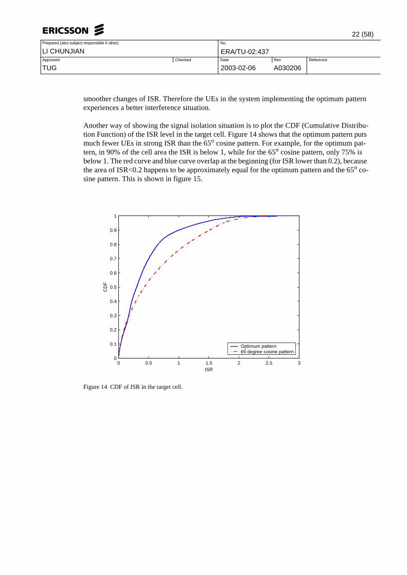
Another way of showing the signal isolation situation is to plot the CDF (Cumulative Distribu-tion Function) of the ISR level in the target cell. Figure 14 shows that the optimum pattern puts much fewer UEs in strong ISR than the 65o cosine pattern. For example, for the optimum pat-tern, in 90% of the cell area the ISR is below 1, while for the 65o cosine pattern, only 75% is below 1. The red curve and blue curve overlap at the beginning (for ISR lower than 0.2), because the area of ISR<0.2 happens to be approximately equal for the optimum pattern and the 65o co-sine pattern. This is shown in figure 15.

Figure 14 CDF of ISR in the target cell.

0 0.5 1 1.5 2 2.5 30

0.1

0.2

0.3

0.4

0.5

0.6

0.7

0.8

0.9

1

ISR

CD

F

Optimum pattern65 degree cosine pattern

Date Rev



2003-02-06 A030206

ERA/TU-02:437

TUG

LI CHUNJIAN

23 (58)

Figure 15 The areas of ISR lower than 0.2 for the two antenna patterns are approximately equal.

A well known parameter for analyzing interference situation in a multi-cell W-CDMA system is the F-factor. F-factor describes the interference level of a multi-cell system with respect to the interference in a single cell. If the F-factor for downlink is defined as [10]

(4)

where is the interference power from all the interfering cells, and is the interference pow-er from the serving cell itself, the overbar means averaging over the cell, the F-factor happens to be equal to the average ISR in the target cell since every basestation transmits the same power. The downlink F-factor for the optimum pattern and 65o cosine pattern is shown in table 3.

Table 3 Downlink F-factors.

The F-factors show that the optimum pattern achieves a 31% reduction in inter-cell interference.

4.5 About the system behavior

4.5.1 Non-unique optimum pattern

There exists different optimum patterns for different load situation, or different power limita-tions. As shown before, optimizing antenna patterns at different loads (from a single UE to 77 UEs), we get different optimum patterns. The one that supports the largest number of users is optimum in the sense of offering the maximum capacity per cell; the other ones are optimum in a sense of radiating least power when supporting their specific load. Curves of power vs. load

The optimum pattern

The 65o cosine pattern

F-factor (Downlink) 0.42 0.61

The area with ISR lower than 0.2, for 65−degree cosine pattern

meter

met

er

0 200 400 600 800 1000 1200 1400 1600 1800 2000

600

400

200

0

−200

−400

−600

−800

meter

met

er

The area with ISR lower than 0.2, for the optimum pattern

0 200 400 600 800 1000 1200 1400 1600 1800 2000

600

400

200

0

−200

−400

−600

−800

FIicIsc------=

Iic Isc

Date Rev



2003-02-06 A030206

ERA/TU-02:437

TUG

LI CHUNJIAN

24 (58)

(number of users) of antenna patterns optimized for different load cross over each other as shown in figure 16. Before crossing point 1 the blue curve (optimum for single UE) is the best choice, after crossing point 2 the red curve (maximum capacity) is the best, and between cross-ing point 1 and 2 the green (optimum for 50 UEs) is the best choice. Similarly, by setting differ-ent finite power limits instead of infinite power, one will also find different optimum patterns. This reminds us that the optimum antenna radiation pattern is subject to the real environment in the network. The optimum pattern that we found here gives the bound at the extreme, thus re-vealing the asymptotic behavior of the system.

Figure 16 Power-load curves for different antenna patterns.

4.5.2 Cell range and capacity trade-off

In a W-CDMA system, the coverage performance and capacity are closely coupled to each other. Therefore the cell range can be traded for capacity or vice versa. In other words, when the num-ber of active users increases, the cell range will be shrinking. This is called cell breathing. As shown in figure 9, to achieve maximum capacity the required total downlink power tends to be infinity. In the finite power limit case, since one can trade the cell range for capacity, it is possi-ble to approach the maximum capacity by shrinking the cell range as depicted in figure 17. At a 2-Watt power limit, 400-meter sites distance, the 65o cosine pattern achieves a capacity of 60 UEs per cell, while the optimum pattern achieves a capacity of 75 UEs, stating a 25% improve-ment. Note that for cell range under 1000 meters the Hata model might not be suitable. We still use the Hata for all cell ranges to show the asymptotic behavior of the system. The crossing of

30 35 40 45 50 55 600

5

10

15

20

25

30

number of UEs

Tot

al d

ownl

ink

pow

er [W

]

The optimum patternOptimized for 50 UEsOptimized for 1 UE

crossingpoint 2

crossing point 1

Date Rev



2003-02-06 A030206

ERA/TU-02:437

TUG

LI CHUNJIAN

25 (58)

the two sets of curves shows the breakeven point in the performance comparison of the two pat-terns. Note that the two sets of curves in the plot always cross over at the same load, i.e. about 38 UEs. That is because the different curves for different power limits are simply scaled versions (along the distance axis) of each other.

Figure 17 Sites distance vs. capacity for different downlink power limits.

4.5.3 The diamond cell shape

The ISR contour plot shows us the actual cell shape produced by the optimum pattern antenna. By drawing lines through the "ridges" of the ISR in a cell, we show the actual cell shape in figure 18. It is not a perfect diamond shape because of the existence of side lobes, but we still call it "the diamond cell shape". As mentioned before, this diamond cell shape has good signal isola-tion properties. It is interesting because it utilizes a relatively narrow beamwidth (60o first null beamwidth) to accomplish coverage in a 3-sectorized system (with sector width of 120o).

10 20 30 40 50 60 70 800

200

400

600

800

1000

1200

1400

1600

1800

2000

Number of UEs

Site

s di

stan

ce [m

eter

]

2W, optimum pattern20W, optimum pattern2kW, optimum pattern2W, 65−degree cosine pattern20W,65−degree cosine pattern2kW,65−degree cosine pattern

Date Rev



2003-02-06 A030206

ERA/TU-02:437

TUG

LI CHUNJIAN

26 (58)

Figure 18 The red line outlines the actual cell shape (for the target cell) produced by the optimum pattern antenna. The target site is located at (0,0).

We learned from this diamond cell shape that two neighboring sites try to avoid pointing their antenna main beams towards the same point on their symmetry line (the line with points having same distances to both sites). By doing this the optimum pattern achieves good site to site signal isolation. Still, there are two points on the symmetry line that are illuminated by both antenna main beams of the neighboring sites, the vertices of the diamond. This is why the ISR is very high at these two vertices.

The sectorization with such antenna patterns and pointing directions can achieve very high sec-torization gain. For comparison, the system capacity using an omni-directional antenna pattern is calculated, which is 64 UEs per site. In a so called perfect sectorization (the three sector-an-tennas have radiation patterns such that no extra interference is introduced), the capacity of the site should be UEs, and the sectorization gain is 3. Using the optimum pattern antenna, the capacity of a sectorized site is UEs, and the sectorization gain is 3.6, much higher than the "perfect sectorization". The extra gain comes from the better signal isolation property of the diamond cell shape.

4.5.4 Comparison of different site plans

If the antenna pointing directions in the Ericsson site plan (figure 5) are rotated 30o it becomes the so called Bell site plan, which is also a commonly used site plan. To investigate the effects of different site plans, we run the optimizer with antenna rotation of 0o, 5o, 10o, 20o, and 30o. The simulations show that with a rotation of 0o (Ericsson site plan), the system achieves highest asymptotic capacity (see table 4).

meter

met

er

−2000 −1500 −1000 −500 0 500 1000 1500 2000

1500

1000

500

0

−500

−1000

−1500

3 64×3 77×

Date Rev



2003-02-06 A030206

ERA/TU-02:437

TUG

LI CHUNJIAN

27 (58)

Table 4 Capacity comparison of different site plans

Note that the asymptotic capacities shown here are produced by different optimum patterns op-timized for the site plans respectively, thus the cell shapes are also different.

4.5.5 Power control

We assume perfect fast power control on downlink. The algorithm is implicitly included in the simulator when setting the same target SIR for every UE. Power control in downlink is impor-tant not only for combating the near-far effect but also for conserving power. Under downlink power control, every UE receives only the power that will maintain the lowest acceptable SIR. To see how the required downlink power varies among UEs we plotted the CDF of the downlink power allocation in a cell in figure 19. It can be seen that the power variation is huge especially for the optimum pattern. The dynamic range of downlink power for the optimum pattern is 19dB while for the 65o cosine pattern it is about 11dB.

Figure 19 The CDF of power allocation at a load of 50 UEs, without HO.

Through figure 19 we can also see the advantage of the optimum pattern. It keeps the downlink power for 92% of UEs lower than W, although the remaining 8% of UEs may require up to W. In contrast, for the 65o cosine pattern, 70% of the UEs require power lower than W, and the rest may require up to W. Recall that we assumed no limit on the DL power.

Antenna rotation 0o 5o 10o 20o 30o

Asymptotic capacity (UEs per cell)

77 68.9 71 69.8 63.7

0 0.5 1 1.5 2 2.5 3

x 10−4

0

0.1

0.2

0.3

0.4

0.5

0.6

0.7

0.8

0.9

1

Downlink power area density [W per unit area]

CD

F

Optimum pattern65−degree cosine pattern

2.5 105–×

2.06 104–×

2.5 105–× 6.31 10

5–×

Date Rev



2003-02-06 A030206

ERA/TU-02:437

TUG

LI CHUNJIAN

28 (58)

To see how the downlink power is allocated at different locations, we plotted the downlink pow-er allocation as a surface, in figure 20 for the optimum pattern and in figure 21 for the 65o cosine pattern. Note that to facilitate comparison of the plots, the peaks of the power surfaces are trun-cated to W if exceed this value, and the maximum color values are set to W for all plots. These two surface plots are also shown in three dimensions in figure 22.

Figure 20 Downlink power allocation on the surface of the cell, for the optimum pattern, at a load of 50 UEs, without HO.

Figure 21 Downlink power allocation on the surface of the cell, for 65o cosine pattern, at a load of 50 UEs, without HO.

8 105–× 8 10

5–×

0

1

2

3

4

5

6

7

8x 10

−5

meter

met

er

0 500 1000 1500 2000

800

600

400

200

0

−200

−400

−600

−800

0

1

2

3

4

5

6

7

8x 10

−5

meter

met

er

0 500 1000 1500 2000

800

600

400

200

0

−200

−400

−600

−800

Date Rev



2003-02-06 A030206

ERA/TU-02:437

TUG

LI CHUNJIAN

29 (58)

Figure 22 3D plots of power allocation for the optimum pattern (up) and the 65-degree cosine pattern (down).

4.5.6 Hand over

When hand over is taken into account, the downlink power for UEs in the HO region is raised because of the introduction of the second-optimum link. We plot the required downlink power in the same way as above but this time with HO (HO margin = 3dB, maximum 3 active links). Comparing figures 23 and 24 with figures 21 and 22, respectively, we can see that HO does not change the power allocation in the diamond cell significantly, while for the cosine pattern HO raises the required power substantially in the HO region. The CDF of downlink power allocation with HO are plotted in figure 25.

Date Rev



2003-02-06 A030206

ERA/TU-02:437

TUG

LI CHUNJIAN

30 (58)

Figure 23 Downlink power allocation on the surface of the cell, for the optimum pattern, at a load of 50 UEs, with HO (3dB margin and maximum 3 active links).

0

1

2

3

4

5

6

7

8x 10

−5

meter

mete

r

0 500 1000 1500 2000

800

600

400

200

0

−200

−400

−600

−800

Date Rev



2003-02-06 A030206

ERA/TU-02:437

TUG

LI CHUNJIAN

31 (58)

Figure 24 Downlink power allocation on the surface of the cell, for 65o cosine pattern, at a load of 50 UEs, with HO (3dB margin and maximum 3 active links).

0

1

2

3

4

5

6

7

8x 10

−5

meter

met

er

0 500 1000 1500 2000

800

600

400

200

0

−200

−400

−600

−800

Date Rev



2003-02-06 A030206

ERA/TU-02:437

TUG

LI CHUNJIAN

32 (58)

Figure 25 The CDF of power allocation at a load of 50 UEs, with HO (3dB HO margin, max. 3 active links). The curves from figure 19 (without HO) are also plotted here, in dotted line, for comparison.

In figure 25 the CDFs without HO are also plotted in dotted lines for comparison. We can see that the effect of HO is that it raises the UE power demand, especially for those UEs located in the HO region, as in figure 25 the highest power demanded per unit area is raised to W for the optimum pattern, and W for the 65o cosine pattern. Since the area with very high power demand is very small, it is not a problem when the propagation environment gives a certain angular spread. Another fact that can be seen clearly is that the HO degrades capacity performance (or DL power performance) more in the 65o cosine pattern case than in the opti-mum pattern case.

0 0.5 1 1.5 2 2.5 3

x 10−4

0

0.1

0.2

0.3

0.4

0.5

0.6

0.7

0.8

0.9

1

Downlink power area density [W per unit area]

CD

F

Optimum pattern without HO65−degree cosine pattern without HOOptimum pattern with HO65−degree cosine pattern with HO

2.3 104–×

1.23 104–×

Date Rev



2003-02-06 A030206

ERA/TU-02:437

TUG

LI CHUNJIAN

33 (58)

5 Achieving maximum capacity with realistic antenna model

To build the optimum pattern antenna that we found in the previous section one needs to use an infinitely large antenna array, which is not practical. In practice, we can use an antenna array with acceptable size (say, one to six columns) to approach the optimum pattern. The radiation pattern of an element column can be modeled by the commonly used cosine pattern, which is called realistic pattern here. The cosine pattern is described in detail in Appendix B.

An antenna array consists of a number of element antennas and thus has higher degree of free-dom to shape its pattern as desired. In this study we use linear antenna arrays with different num-bers of elements and different excitation amplitude to the elements. The overall radiation pattern of such an array is described by the array factor (AF) and the element factor (EF), which are also shown in Appendix B.

The simulations show that for a single column antenna, 35o beamwidth gives highest capacity (in a 5o resolution). It is actually 38o if calculated in 2o resolution as depicted in figure 26, but we still use 5o resolution complying to the previous context. Only slight improvement is achieved by using more columns (2, 3, 4 and 6). Consequently, the following analysis is made with a single column antenna. Figure 26 shows that with a 35o 3dB-beamwidth, the single col-umn antenna achieves the maximum capacity of 69 users per cell.

Figure 26 Downlink capacity versus beamwidth, without HO, for a single column antenna with cosine shape element pattern.

As mentioned above, with different load, the optimum beamwidth is different for the same sys-tem. Figure 27 shows this characteristic.

0 20 40 60 80 100 12030

35

40

45

50

55

60

65

70

3 dB beamwidth [degrees]

Cap

acity

(max

imum

no.

of u

sers

per

cel

l)

Date Rev



2003-02-06 A030206

ERA/TU-02:437

TUG

LI CHUNJIAN

34 (58)

Figure 27 Total downlink power per cell as a function of half-power beamwidth, without HO. Parameter is the load in the cell. Circles indicate the optimum for each load, i.e. the beamwidth giving the lowest output power.

We can see that at very low load (10 UEs), the optimum beamwidth is about 70o, and in a wide range around 70o it is quite flat. When the number of active UEs in the cell increases, the opti-mum becomes less flat and the optimum beamwidth becomes smaller. At 35o it achieves the highest capacity 69 UEs.

Letting site distance be a variable, in figure 28, we see that at a 2-Watt power limit and 400-meter site distance, the 35o pattern outperforms the 65o pattern by 15%. Again, the crossings of the two set of curves show the breakeven points in the performance comparison of the two pat-terns.

0 20 40 60 80 100 12010

−1

100

101

102

103

104

105

3dB−beamwidth [degree]

Tota

l dow

nlin

k po

wer

[W]

10 UEs30 UEs50 UEs60 UEs69 UEsThe minimum

Date Rev



2003-02-06 A030206

ERA/TU-02:437

TUG

LI CHUNJIAN

35 (58)

Figure 28 Site distance versus capacity for fixed downlink power, without HO.

We also plot F-factor with respect to the 3dB-beamwidth, as shown in figure 29. It can be seen that the beamwidth producing lowest F-factor is also 35o.

Figure 29 Downlink F-factor vs. 3dB-beamwidth.

10 20 30 40 50 60 700

200

400

600

800

1000

1200

1400

1600

1800

2000

Number of UEs

Site

s di

stan

ce [m

eter

]

2 W, 35 degree20 W, 35 degree2 kW, 35 degree2 W, 65 degree20 W, 65 degree2 kW, 65 degree

30 40 50 60 70 80 90 1000.45

0.5

0.55

0.6

0.65

0.7

0.75

0.8

0.85

0.9

3dB beamwidth [degree]

Dow

nlin

k F

−fa

ctor

Date Rev



2003-02-06 A030206

ERA/TU-02:437

TUG

LI CHUNJIAN

36 (58)

A comparison of the CDF curves for the ISR of the optimum pattern, the 35o cosine pattern, and the 65o cosine pattern is shown in figure 30. It is obvious from figure 30 that the cell isolation is improved using 35o instead of 65o beamwidth cosine pattern.

Figure 30 Comparison of CDF of ISR for three antenna patterns.

To see how the optimum beamwidth changes with different antenna pointing directions, we plot the capacity vs. beamwidth curve for the Ericsson plan as well as other six rotated site plan, in figure 31. It shows that when the rotation increases the optimum beamwidth is getting larger and the asymptotic capacity is lowered. Figure 31 also shows that the narrower beams are more sen-sitive to the antenna rotations than the wider beams.

0 1 2 3 4 5 60

0.1

0.2

0.3

0.4

0.5

0.6

0.7

0.8

0.9

1

ISR

CD

F

Optimum pattern35−degree cosine pattern65−degree cosine pattern

Date Rev



2003-02-06 A030206

ERA/TU-02:437

TUG

LI CHUNJIAN

37 (58)

Figure 31 Capacity vs. beamwidth for different antenna pointing direction. 0-degree rotation stands for the Ericsson site plan and 30-degree rotation stands for the Bell site plan.

10 20 30 40 50 60 70 80 90 10020

25

30

35

40

45

50

55

60

65

70

3dB−beamwidth

capa

city

0−degree rotation5−degree rotation10−degree rotation15−degree rotation20−degree rotation25−degree rotation30−degree rotation

Date Rev



2003-02-06 A030206

ERA/TU-02:437

TUG

LI CHUNJIAN

38 (58)

6 Hand over and other issues

As mentioned before, hand over has the effect of decreasing system capacity in downlink from a power allocation point of view. Both soft and softer hand over also occupy extra system re-sources, like the channelization codes, which is of limited number in a cell. So it is important to understand how the different antenna patterns affect the number of UEs in HO. Figure 32 shows that to have a minimum number of UEs in HO we should choose an antenna beamwidth of around 25o, which is very narrow compared to the 65o cosine reference pattern.

Figure 32 Handover percentage versus beamwidth for cosine patterns.

To see how the UEs in SHO or SrHO are distributed in the cell, or, in what area the UEs will be switched to SHO or SrHO mode, a HO "map" is needed. A comparison of the HO situations for the optimum pattern, 35o cosine pattern, and 65o cosine pattern is shown by figures 33, 34 and 35.

By letting less UEs in HO, the optimum pattern outperforms the 65o cosine pattern in terms of capacity, even more than 27% as we have shown without HO, because of the aforesaid reasons. Less SHO UEs also conserves the data traffic between HO base stations. The drawback of small HO region is the difficulty of processing HO. From figure 33 we can see the smallest distance for a UE to perform SHO is about 10 meters. This is difficult for a fast moving UE but suitable for pedestrian users.

0 20 40 60 80 100 1200

0.05

0.1

0.15

0.2

0.25

0.3

0.35

0.4


perc

enta

ge o

f HO

3dB HO margin

soft&softer softer

Date Rev



2003-02-06 A030206

ERA/TU-02:437

TUG

LI CHUNJIAN

39 (58)

Figure 33 HO area with the optimum pattern, with 3dB HO margin. Blue: no HO, green: in SHO, brown: in SrHO.

Figure 34 HO area with the 35o cosine pattern, with 3dB HO margin. Blue: no HO, green: in SHO, brown: in SrHO.

meter

met

er

The optimum pattern: 6.6% in SHO, 0.07% in SrHO

0 200 400 600 800 1000 1200 1400 1600 1800 2000

600

400

200

0

−200

−400

−600

35 degree cosine pattern: 12.4% in SHO, 0.5% in SrHO

meter

met

er

0 200 400 600 800 1000 1200 1400 1600 1800 2000

600

400

200

0

−200

−400

−600

Date Rev



2003-02-06 A030206

ERA/TU-02:437

TUG

LI CHUNJIAN

40 (58)

Figure 35 HO area with 65o cosine pattern, with 3 dB HO margin. Blue: no HO, green: in SHO, brown: in SrHO.

The impact on capacity by HO for different beamwidth is shown in figure 36. It is clear that HO lowers capacity, and reduces the optimum beamwidth slightly because the beamwidth minimiz-ing HO is small (about 25o). In 5o resolution there is no difference in optimum beamwidth.

Figure 36 Asymptotic capacity vs. 3dB beamwidth, with and without HO. HO margin=3dB.

meter

met

er

65 degree cosine pattern: 19.2% in SHO, 1.4% in SrHO

0 200 400 600 800 1000 1200 1400 1600 1800 2000

600

400

200

0

−200

−400

−600

0 20 40 60 80 100 120

30

35

40

45

50

55

60

65

70

Cap

acity

(m

axim

um n

o. o

f use

rs p

er c

ell)


Without HOWith HO

Date Rev



2003-02-06 A030206

ERA/TU-02:437

TUG

LI CHUNJIAN

41 (58)

7 Uplink analysis

To justify the antenna optimization described in the previous sections from the whole system viewpoint, we need to examine the uplink capacity and power relation as well. This section will start from introducing an uplink power equation, then simulations based on the equation will be used to analyze the uplink optimum.

7.1 Uplink power equation

Using the same interference model and system parameters as in the downlink analysis, the up-link capacity can be expressed as a function of base station received power:

(5)

where K is the base station received power from a UE connecting to the base station, g1(x,y) is the effective path gain from a UE at location (x,y) in the target cell (cell 1) to the antenna of the target cell, gc(x,y) is the effective path gain from a UE at the same relative location in cell c as g1(x,y) in the target cell to the antenna of target cell, is the surface of target cell, and A is the area of target cell. K is a constant for all UEs because we assume uniform service and perfect uplink power control:

(6)

where Pn is the uplink power for UE n, gn is the path gain from UE n to the serving cell. The derivation of equation (5) is shown in Appendix D. By setting K to infinity (or a large value) we are able to find the maximum number of UEs per cell, with a certain antenna pattern.

By rearranging equation (5), we have an equation expressing K in terms of the number of UEs per cell

(7)

Once K is known, the individual uplink power for every UE can be calculated by the relation shown in equation (6).

Nu

GPK

SIR---------- N0–

KA----

gc x y,( )c 1=

C∑g1 x y,( )

------------------------------------- ΩdΩ∫

------------------------------------------------------=

Ω

P1g1 P2g2 … Pngn K= = = =

K

N0SIR

Gp-----------------

1SIR Nu

GPA------------------

gc x y,( )c 1=

C∑g1 x y,( )

------------------------------------- ΩdΩ∫–

-----------------------------------------------------------------------------=

Date Rev



2003-02-06 A030206

ERA/TU-02:437

TUG

LI CHUNJIAN

42 (58)

7.2 Simulation results

Note that uplink receiver diversity is not included in this study since we assume one base station antenna.

Firstly we show how the uplink capacity varies with different uplink data rates by the power-load curves in figure 37. The power-load curves are different for uplink from that of downlink in that the power axis represents the UE power limit (the maximum power that a UE can trans-mit, usually only the UE located at a position that has worst path gain transmits at the power limit) in the uplink case, while in downlink it represents the total base station output power in a cell. By letting the UE power limit go to infinity, we find the asymptotic capacity bound of up-link. For example, at a data rate of 9.6kbps, the UL asymptotic capacity for the optimum pattern is 49 UEs per cell, and 43 for the 65o cosine pattern.

Figure 37 The UL power-load curves for different data rates and different patterns.

We then find an optimum realistic single column antenna for UL. Figure 38 shows that the op-timum base station antenna beamwidth for uplink is approximately the same for downlink, i.e., about 35o.

0 10 20 30 40 50 60 70 80 90 10010

−1

100

101

102

103

104

105

Capacity per cell

UL

pow

er li

mit

[W]

Optimum pattern, 12.2kbpsOptimum pattern, 9.6kbpsOptimum pattern, 4.8kbps65−degree cosine pattern,12.2kbps65−degree cosine pattern,9.6kbps65−degree cosine pattern,4.8kbps

Date Rev



2003-02-06 A030206

ERA/TU-02:437

TUG

LI CHUNJIAN

43 (58)

Figure 38 UL capacity versus beamwidth (cosine pattern), at 9.6kbps, infinite power. Dashed line shows the UL capacity bound (given by the optimum pattern).

This result shows that the optimum beamwidth for DL is also the optimum beamwidth for UL, based on the assumption of infinite downlink and uplink power.

0 20 40 60 80 100 12025

30

35

40

45

50


Cap

acity

per

cel

l

Date Rev



2003-02-06 A030206

ERA/TU-02:437

TUG

LI CHUNJIAN

44 (58)

8 Comparison with previous study

Optimum antenna beamwidth has been studied before, for example [4] and [5]. In those studies, it was found that, for a three-sectorized multicell W-CDMA system with the Ericsson site plan, the optimum 3dB-beamwidth is about 65o(for downlink), which is much larger than what we have found in this study. It was also found that the optimum antenna beamwidth for downlink is different from that of uplink. The reason behind these differences is the different definitions or approaches to the optimum beamwidth.

In [4] the downlink antenna optimum is defined as the antenna parameters yielding a minimum of the transmitted power at a certain load, while in this study the definition of optimum antenna pattern for maximum capacity is the antenna parameters yielding highest capacity assuming in-finite downlink power. These two definitions will definitely produce different optimum beam-width as is discussed in section 4.5 and also shown in figure 27.

In [5], the approach is based on setting a finite downlink power limit and a certain site distance, which is also shown to produce different results from those found in this study. In this study we assume infinite downlink power, to obtain the asymptotic behavior of the system. In uplink we also assume infinite power limit for UEs, so that the uplink optimum is also found in an asymp-totic sense.

It is shown in this report that the optimum beamwidth for both uplink and downlink are in agree-ment, and this can only be true in an asymptotic sense. Besides, by such an asymptotic approach we get insights into the coverage-capacity interaction of a W-CDMA system which is not avail-able in the two previous studies since they fixed power and site range.

Date Rev



2003-02-06 A030206

ERA/TU-02:437

TUG

LI CHUNJIAN

45 (58)

9 Conclusion

An antenna radiation pattern has been found which is optimum with respect to downlink capac-ity performance. The optimum pattern is modeled as piecewise-linear and achieves highest ca-pacity per cell, with a 27% improvement over a reference pattern, which is a 65o cosine pattern. The optimum piecewise-linear pattern gives a theoretical capacity upper bound, which can serve as a benchmark when analyzing other antenna patterns.

By assuming infinite downlink power, the simulation shows some interesting system behavior and gives the asymptotic system capacity. The asymptotic capacity is of theoretical importance, even though it is not available in a practical system, not only because it gives the capacity bound, but also because the optimum pattern found based on maximizing-asymptotic-capacity criterion is independent of actual basestation power limit, antenna gain, and site distance. Thus the opti-mum pattern found in this paper is more general than those results found by criterion with fixed power limit, antenna gain, and site distance.

Using realistic antenna arrays with various sizes to approach the performance of the optimum pattern, we found that a single column antenna with 35o beamwidth (modeled by cosine pattern) achieves 15% improvement over the reference pattern in terms of asymptotic downlink capacity. No significant extra improvement is seen when using more than one column.

Soft handover as well as softer handover occupy extra system resources and require more down-link power and thus have a negative impact on downlink capacity performance. We show how the antenna patterns affect HO by calculating the HO percentage for different patterns. The re-sult shows that a 25o cosine pattern minimizes the percentage of HO users in a multicell system, and the 35o cosine pattern has 40% less HO users than the reference pattern has. This is good for capacity but might pose difficulty in processing HO because of very small HO regions.

Finally, the uplink study shows that the optimum beamwidth (35o 3dB-beamwidth) for down-link capacity is also the optimum beamwidth for uplink. The optimum beamwidth improves the uplink capacity by 9% over the reference pattern. So no compromise between uplink and down-link performance is needed when choosing an optimum beamwidth for the whole system.

Date Rev



2003-02-06 A030206

ERA/TU-02:437

TUG

LI CHUNJIAN

46 (58)

10 Future work

The following relevant topics are interesting but not treated in this study. These topics suggest studying the optimum pattern in more realistic environment and with extension to higher dimen-sion model and highly sectorized system.

It is interesting to study the optimum pattern or optimum beamwidth for 6 (or higher)-sectorized systems, to investigate if the advantage of the diamond cell shape is retained in the 6-sectors sys-tem. Such a study will also show how the isolation gain changes with increasing number of sec-tors.

It is interesting to apply more realistic path loss models by including, for example, shadow fad-ing, multipath fading and angular spread.

Three-dimensional optimum radiation pattern study is also interesting. Combining the optimi-zation for both elevation pattern and azimuthal pattern may give even better performance.

Date Rev



2003-02-06 A030206

ERA/TU-02:437

TUG

LI CHUNJIAN

47 (58)

References

[1] W. C. Y. Lee and D. J. Y. Lee, "CDMA System Capacity Analysis", 12th IEEE International Symposium on Personal, Indoor and Mobile Radio Communications.

[2] S. Dehghan, D. Lister, R. Owen, and P. Jones, "W-CDMA Capacity and Planning Issues", Electronics & Communication Engineering Journal. June 2000; 12(3): 101-18.

[3] R. Padovani, B. Butler, R. Boesel, "CDMA digital cellular: field test result", VTC 1994. ‘Creating Tomorrow’s Mobile Systems’. 1994 IEEE 44th Vehicular Technology Conference Cat. No.94CH3438-9. 1994: 11-15 vol.1.

[4] P. Fornmark, Ericsson internal report 61/0363-FCK 115 02 Uen, Rev A, 2000-01-24.

[5] B. Christer V. Johansson and S. Stefansson, "Optimizing Antenna Parameters for Sectorized W-CDMA Network", IEEE VTS Fall VTC2000.

[6] M. Johansson, Ericsson internal report T/U-01:124, 2001-08-22.

[7] W. Huyer and A. Neumaier, "Global optimization by multilevel coordinate search", Global Optimization 14 (1999), 331-355.

[8] T. S. Rappaport, Wireless Communications Principles & Practice, Prentice Hall, 1996.

[9] J. Korhonen, Introduction to 3G Mobile Communications, Artech House, 2001.

[10] Ericsson internal report, 17/1551-HSD 101 02/1.

Date Rev



2003-02-06 A030206

ERA/TU-02:437

TUG

LI CHUNJIAN

48 (58)

Terminology

CDF Cumulative Distribution Function

DL Downlink

EMF Electromagnetic field

ISR Interfering-cells-path-gain to serving-cell-path-gain ratio

MAI Multiple access interference

MRC Maximum ratio combining

SHO Soft hand over

SIR Signal to interference ratio

SINR Signal to interference and noise ratio

SLL Side lobe level

SrHO Softer hand over

UE User equipment

UL Uplink

W-CDMA Wideband code division multiple access

Date Rev



2003-02-06 A030206

ERA/TU-02:437

TUG

LI CHUNJIAN

49 (58)

0

-

Appendix A : Downlink power equations

A.1 Discrete user-distribution approach without handover

In this section the analytical expression for SINR (signal-to-interference-and-noise ratio) of a UE is given first, then the capacity of the cell is related to total downlink output power.

Assume there is a total of R sites in the site plan, each site is divided into S cells, and in cell number s of site r there are Nu

s,r users arbitrarily distributed over the area of the cell. Let cell 1 in site 1 be the target cell. The SINR (for brevity hereafter SINR is written as SIR) for UE num-ber n in the target cell can be written as

(A.1)

where Ps,rn and Gs,r

pn are the downlink output power and processing gain, respectively, for UE number n in cell s at site r, gr,s,n is the effective path gain ( antenna gain, path loss, and fading) for the signal path between sector s at site r and UE number n in the target cell, is the orthog-onality factor, and N0 is the noise power. if we assume identical UE distribution in every cell, it is not necessary to distinguish UEs with different cell notation. The above equation (A.1) can then be simplified as

(A.2)

(A.3)

To make the notation more compact, the effective path gain can be identified by only cell se-quence number (without explicit reference to sites). Then the equation becomes

SIRn1 1, Pn

1 1, Gpn1 1, g1 1 n, ,

1 α–( )g1 1 n, , Pn’1 1, Pn’

s 1, g1 s n, , Pn’s r, gr s n, , N+

n’ 1=

Nus r,

∑s 1=

S

∑r 2=

R

∑+

n’ 1=

Nus 1,

∑s 2=

S

∑+

n’ 1=

Nu1 1,

∑

------------------------------------------------------------------------------------------------------------------------------------------------------------------------------------------=

α

SIRn

PnGpng1 1 n, ,

1 α–( )g1 1 n, , Pn’ Pn’g1 s n, , Pn’gr s n, , N0+

n’ 1=

Nu

∑s 1=

S

∑r 2=

R

∑+

n’ 1=

Nu

∑s 2=

S

∑+

n’ 1=

Nu

∑

----------------------------------------------------------------------------------------------------------------------------------------------------------------------------------=

PnGpng1 1 n, ,

αg1 1 n, ,– gr s n, ,

s 1=

S

∑r 1=

R

∑+

Pn’ N0+

n’ 1=

Nu

∑

------------------------------------------------------------------------------------------------------=

SIRPnGpng1 n,

1 α–( )g1 n, Pn’ Pn’gc n, N0+

n’ 1=

Nu

∑c 2=

C

∑+

n’ 1=

Nu

∑

------------------------------------------------------------------------------------------------------------=

Date Rev



2003-02-06 A030206

ERA/TU-02:437

TUG

LI CHUNJIAN

50 (58)

(A.4)

where gc,n is the effective path gain for the signal path between basestation antenna in cell c and UE number n in the target cell (cell number 1), and C is the total number of cells in the system. Rewrite (A.4) to get the downlink output power for a specific UE n, the Pn, as

(A.5)

where Ptot (= ) is the total downlink output power per cell. Summing over all Pn in (A.5) and solving for Ptot , we get a closed-form expression for the total downlink output power per cell:

. (A.6)

One way of calculating the capacity (maximum number of users) [6] is to evaluate (A.6) for in-creasing N until the total power Ptot reaches a predetermined value, which maybe finite or infi-nite. In the case of infinite power, the capacity is only limited by the interference level in the system, while thermal noise power does not affect it.

Applying infinite downlink power in the equation is of significance when the asymptotic system behavior is of interest. Because the downlink power is dependent on site spacing and terrain, a specific power limit can only give us knowledge about the capacity under a certain scenario, while infinite power let us know the upper-bound of the capacity.

When infinite power is applied, the maximum capacity (or, asymptotic capacity) can be evalu-ated by setting the denominator of (A.6) to 0. If uniform service is assumed, then SIRn=SIR and Gpn=Gp . The equation for infinite power can then be further simplified:

. (A.7)

Because the users are discrete (the number of users can only be an integer) and randomly dis-tributed, one needs to evaluate the capacity based on a large number of user distributions and then take the average.

PnGpng1 n,

αg1 n,– gc n,

c 1=

C

∑+

Pn’ N0+

n’ 1=

Nu

∑

-------------------------------------------------------------------------------------=

Pn

SIRn

Gpng1 n,--------------------- N0 Ptot gc n, αg1 n,–

c 1=

C

∑

+=

Pn’∑

Ptot

N0SIRn

Gpng1 n,---------------------

n 1=

Nu

∑

1SIRn

Gpn------------- α

gc n,g1 n,----------

c 1=

C

∑–

n 1=

Nu

∑+

-----------------------------------------------------------------------=

Gp

SIR---------- Nuα–

gc n,g1 n,----------

c 1=

C

∑n 1=

Nu

∑+=

Date Rev



2003-02-06 A030206

ERA/TU-02:437

TUG

LI CHUNJIAN

51 (58)

A.2 Continuous user-distribution approach without handover

If we allow the number of users to be a continuous variable and represent the cell capacity as a UE density on the surface of the cell area, (A.5) can be generalized to represent the required power at any point of the target cell, P(x,y). Replacing the discrete UE index n with a depen-dence on spatial coordinates for all quantities, i.e., replacing summation over n with integral over area, the expression for the power density P(x,y) becomes

(A.8)

where is a normalized UE distribution, i.e.,

with being the unit cell with best effective path gain, Nu is the non-integer number of users per cell, and

Integrating (A.8) over the unit cell, and solving for Ptot , we get an expression for the total output power per cell:

(A.9)

For uniform traffic and service, we can simplify the equation by representing UEs with a uni-form surface density , where A is the area of a single unit cell, and letting SIR(x,y)=SIR and Gp(x,y)=Gp. It reduces to

(A.10)

Similarly, the expression for maximum capacity reduces to

P x y,( )SIR x y,( )η x y,( )Nu

Gp x y,( )g1 x y,( )-------------------------------------------------- N0 Ptot gc x y,( ) αg1 x y,( )–

c 1=

C

∑

+=

η x y,( )

η x y,( ) ΩdΩ1∫ 1=

Ω1

Ptot P x y,( ) ΩdΩ1∫=

Ptot

N0NuSIR x y,( )η x y,( )Gp x y,( )g1 x y,( )------------------------------------------- Ωd

Ω1∫

1 NuSIR x y,( )η x y,( )

Gp x y,( )------------------------------------------- α

gc x y,( )g1 x y,( )--------------------

c 1=

C

∑–

ΩdΩ1∫+

-------------------------------------------------------------------------------------------------------------------------=

η x y,( ) 1 A⁄=

Ptot

N01A---- 1

g1 x y,( )-------------------- Ωd

Ω1∫

Gp

SIR Nu------------------ α 1

A----

gc x y,( )g1 x y,( )--------------------

c 1=

C

∑

ΩdΩ1∫–+

------------------------------------------------------------------------------------------=

Date Rev



2003-02-06 A030206

ERA/TU-02:437

TUG

LI CHUNJIAN

52 (58)

(A.11)

A.3 Handover

Assuming MRC (maximum ratio combining) at the UEs, the effective SIR value, in the presence of handover, is the sum of the SIR values of the individual link. For the discrete user case, the SIR equation can be rewritten

(A.12)

where Ln is the number of active handover links for UE number n. Note that all links for a given UE n are assumed to require the same output power Pn. Here it is impossible to solve for Ptot by summing all Pn because of the summation of individual SIR terms (one for each HO link). To be able to solve it, we let all denominators in (A.12) equal by replacing the effective path gain for the active links in the denominator with the geometric mean of them. Then we get an approx-imation:

(A.13)

For all practical purposes, using the geometric mean will produce results that are very close to that of the exact expression in (A.13). The approximation performs worst in the case of a single UE connected via two links when interference exceeds the noise (an interference-limited sce-nario with extremely low load!). Even then, the maximum error is less than 3% for a handover margin of 3 dB (with ); for any realistic scenario, the errors will be only fractions of one percent, which is insignificant for our purposes.

We rewrite (A.13) to get the total output power Pn for a specific UE n (for all handover links) as

Nu

Gp

SIR----------

α–1A----

gc x y,( )g1 x y,( )--------------------

c 1=

C

∑ ΩdΩ1∫+

-----------------------------------------------------------------=

SIRn

PnGpn

Ln-----------------

gc’ n,

αgc’ n,– gc n,

c 1=

C

∑+

Ptot N0+

----------------------------------------------------------------------------

c’ 1=

Ln

∑=

SIRn

PnGpn

Ln----------------- gc’ n,

c’ 1=

Ln

∑

Ln α–( ) gc’ n,

c’ 1=

Ln

∏

1Ln-----

gc n,

c Ln 1+=

C

∑+ Ptot N0+

-----------------------------------------------------------------------------------------------------------------------≈

α 0.3 0.7,[ ]∈

Date Rev



2003-02-06 A030206

ERA/TU-02:437

TUG

LI CHUNJIAN

53 (58)

(A.14)

Summing over all Pn in (A.14), and solving for Ptot, we get an expression for the total output power per cell:

(A.15)

For the continuous user distribution case, by the same way, we get the following

(A.16)

And the expression for maximum capacity reduces to

(A.17)

Pn

LnSIRn

Gpn gc’ n,

c’ 1=

Ln

∑

--------------------------------- Ln α–( ) gc’ n,

c’ 1=

Ln

∏

1Ln-----

gc n,

c Ln 1+=

C

∑+ Ptot N0+

=

Ptot

N0LnSIRn

Gpn gc’ n,c’ 1=

Ln∑----------------------------------------

n 1=

Nu

∑

1L SIR

Gpn gc’ n,c’ 1=

Ln∑⋅-------------------------------------------- Ln α–( ) gc’ n,

c’ 1=

Ln

∏

1Ln-----

gc n,

c Ln 1+=

C

∑+

n 1=

Nu

∑–

-----------------------------------------------------------------------------------------------------------------------------------------------------------------=

Ptot

N01A---- L x y,( )

gc’ x y,( )c’ 1=

L x y,( )∑------------------------------------------ Ωd

Ω1∫

Gp

SIR Nu------------------ 1

A---- L x y,( )

gc’ x y,( )c’ 1=

L x y,( )∑------------------------------------------ L x y,( ) α–( ) gc’ x y,( )

c’ 1=

L x y,( )

∏

1L x y,( )-----------------

gc x y,( )c L x y,( ) 1+=

C

∑+ ΩdΩ1∫–

--------------------------------------------------------------------------------------------------------------------------------------------------------------------------------------------------------------------------------------------=

Nu

Gp SIR( )⁄

1A---- L x y,( )

gc’ x y,( )c’ 1=

L x y,( )∑------------------------------------------ L x y,( ) α–( ) gc’ x y,( )

c’ 1=

L x y,( )

∏

1L x y,( )-----------------

gc x y,( )c L x y,( ) 1+=

C

∑+ ΩdΩ1∫

-------------------------------------------------------------------------------------------------------------------------------------------------------------------------------------------------------------------=

Date Rev



2003-02-06 A030206

ERA/TU-02:437

TUG

LI CHUNJIAN

54 (58)

Appendix B : The antenna model

The element factor (EF) of an antenna array describes the radiation amplitude pattern of an el-ement column constituting the array. The cosine shape is widely used:

(B.1)

where the exponential

(B.2)

produces the desired half-power beamwidth .

The amplitude radiation pattern of the antenna array is modeled by EF and the Array Factor (AF)

(B.3)

where

(B.4)

where N is the number of columns constituting the array, and an is the excitation amplitude of the nth column. By squaring (B.4), we got the gain (power) radiation pattern of a antenna array, which is used in the following section to approach the optimum patterns. The normalization of the gain pattern is also needed here to make different patterns comparable. The gain pattern of a single column realistic antenna with 65o 3dB-beamwidth is plotted in figure 3.

EF φ( ) COSn φ2--- =

n 3

20φ3dB

4----------- coslog

------------------------------------------------–=

φ3dB

f φ( ) EF φ( )AF φ( )=

AF φ( ) anej2πλ---yn φ( )sin

n 1=

N

∑=

Date Rev



2003-02-06 A030206

ERA/TU-02:437

TUG

LI CHUNJIAN

55 (58)

Appendix C : Simulation parameters

Table C.1 The site geometry.

Table C.2 The link level parameters.

Site spacing 2000 meters

Sector antenna direction

see figure 4

Base station antenna height

30 meters

UE antenna height 3 meters

Propagation model Hata model:

C1=141dB, C2=35dB

Slow or fast Fading not considered

Working frequency 2110 MHz

Antenna Side Lobe Level (SLL)

-30dB

Noise figure 9 dB

Base station transmission loss

2 dB

L dB( ) C1 C2 dlog+=

Date Rev



2003-02-06 A030206

ERA/TU-02:437

TUG

LI CHUNJIAN

56 (58)

Table C.3 The system parameters.

Chip rate 3.84 Mchip/s

Information bite rate 12.2 kbit/s

Target SIR 7.6 dB

Downlink orthogonality 0.7

Voice activity 1

Active set size in soft handover

3

Handover margin 3 dB

Date Rev



2003-02-06 A030206

ERA/TU-02:437

TUG

LI CHUNJIAN

57 (58)

Appendix D: Uplink power equation

According to the interference model defined in section 2.1.1, the uplink SIR for UE n can be written as

(D.1)

where Nu is the number of UEs per cell, Pn is the transmitted power of UE n, gc,n is the effective path gain from UE n in cell c to the antenna of the target cell (cell 1), and N0 is the noise power. Assuming uniform services and perfect power control, then SIRn=SIR and

(D.2)

and (D.1) can be written as

(D.3)

Assuming continuous user distribution, the first summation in the denominator can be replaced by the UE density multiplied by an integral

(D.4)

where A is the area of the cell, is the cell surface. Solving (D.4) for the capacity Nu we get

(D.5)

which is the final equation for evaluating capacity in uplink.

SIRn

Png1 n, GP

Pn’ gc n’, N0+c 1=

C∑n’ 1=

Nu∑--------------------------------------------------------------------=

P1gc 1, P2gc 2, … Pngc n, K= = = =

SIRGPK

kg1 n’,----------- gc n’, N0+

c 1=

C∑n’ 1=

Nu∑------------------------------------------------------------------------=

SIRGPK

KNu

A-----------

gc x y,( )c 1=

C∑g1 x y,( )

------------------------------------- ΩdΩ∫ N0+

---------------------------------------------------------------------------=

Ω

Nu

GPK

SIR------------ N0–

KA----

gc x y,( )c 1=

C∑g1 x y,( )

------------------------------------- ΩdΩ∫

------------------------------------------------------=

Date Rev



2003-02-06 A030206

ERA/TU-02:437

TUG

LI CHUNJIAN

58 (58)

efficient antenna patterns for three- sector wcdma systemswcdma systems master of science thesis by...

Documents