HAL Id: hal-01689868https://hal.inria.fr/hal-01689868

Submitted on 22 Jan 2018

HAL is a multi-disciplinary open accessarchive for the deposit and dissemination of sci-entific research documents, whether they are pub-lished or not. The documents may come fromteaching and research institutions in France orabroad, or from public or private research centers.

L’archive ouverte pluridisciplinaire HAL, estdestinée au dépôt et à la diffusion de documentsscientifiques de niveau recherche, publiés ou non,émanant des établissements d’enseignement et derecherche français ou étrangers, des laboratoirespublics ou privés.

Efficient Decentralized Collaborative Mapping forOutdoor Environments

Luis Contreras-Samamé, Olivier Kermorgant, Philippe Martinet

To cite this version:Luis Contreras-Samamé, Olivier Kermorgant, Philippe Martinet. Efficient Decentralized CollaborativeMapping for Outdoor Environments. International Conference on Robotic Computing, Jan 2018,Laguna Hills, United States. �hal-01689868�

Efficient Decentralized Collaborative Mapping for OutdoorEnvironments

Luis Contreras, Olivier Kermorgant and Philippe Martinet

Abstract—An efficient mapping in mobile robotics may involvethe participation of several agents. In this context, this articlepresents a framework for collaborative mapping applied tooutdoor environments considering a decentralized approach. Themapping approach uses range measurements from a 3D lidarmoving in six degrees of freedom. For that case, each robotperforms a local SLAM. The maps are then merged whencommunication is available between the mobile units. This allowsbuilding a global map and to improve the state estimation of eachagent. Experimental results are presented, where partial maps ofthe same environment are aligned and merged coherently in spiteof the noise from the lidar measurement.

I. INTRODUCTION

In the area of mobile robots, many tasks are related withexploration and re-construction of the environments. Thesetasks involve problems as Simultaneous Localization andMapping (SLAM), in which the mobile robot is placed inan unknown environment and must estimate the map of itssurroundings as well as its pose (position and orientation)relative to the map. This is a complex task since determiningthe robot’s localization typically requires prior knowledge ofits surroundings, and on the other hand, map building of itssurroundings requires knowledge of the robot’s localization.In order to build a map, the robot has to traverse the unknownenvironment and incrementally collect measurements of itssurroundings and new pose. Furthermore, the presence ofuncertainty and noise in the measurements from the sensors,produces accumulate errors over time that consequently distortthe robots estimate of its position and map.

The mapping of a large area may require the use of a groupof robots that build the maps in a reasonable amount of timeconsidering accuracy in the map construction [1]. So, a setof robots extends the capability of a single robot by mergingmeasurements from group members, providing each robot withinformation beyond their individual sensors range. This allowsa better usage of resources and executes tasks which are notfeasible by a single robot. Multi-robot mapping is consideredas a decentralized approach when each robot builds their localmaps independently of one another and merges their mapsupon rendezvous. On the other hand, a centralized approachwould require all data to be merged at a single computationunit.

The proposal of this article is a collaborative decentralizedmapping framework for efficient merging of 3D maps (seeFigure 1 ) where:• In the first stage named “Pre-Local Mapping”, each indi-

vidual robot builds its map and sends a certain part of it to

The authors are from the Laboratoire des Sciences du Numeriquede Nantes (LS2N), Ecole Centrale de Nantes (ECN), France.Emails: {Luis.Contreras, Olivier.Kermorgant,Philippe.Martinet}@ls2n.fr

This article is based upon work supported by the Sustain-T ErasmusMundus Project.

Fig. 1. Architecture of our Collaborative Decentralized Mapping System

the other robots based on our proposed Sharing algorithm.Low-cost GPS data is used for the first alignment betweenmaps represented in a global frame.

• For the second stage named “Local Mapping”, the reg-istration process considers the first alignment previouslymentioned and includes an intersecting technique of mapsto reduce the required bandwidth.

This article is organized as follows: Section II presentsthe current works developed in this field. We then detail ourapproach in Section III. Finally, experimental results arepresented and analyzed in Section IV, from data acquired onthe campus of cole Centrale de Nantes.

II. RELATED WORKS

One of the topic to consider in mapping is the type ofsensor used in the robot navigation. In this context, lidarhas become a useful range sensor for these applications [2][3]. Nonetheless, when the lidar scan rate is higher than itstracking, distortion may occur in the map building. In thiscase, standard registration methods as ICP [4] can be appliedto match laser returns for different scans.

Bosse and Zlot [5] [6] [7] use a 2-axis lidar and matchesgeometric structures of a set local point generated by thelidar in order to build a point cloud [7]. The mapping systemincludes an IMU and uses loop closure to reconstruct largemaps. This approach is based on batch processing to buildmaps with accuracy and hence is not applicable to real-timemapping.

In the proposed approach, we consider a Pre-Local Mappingstage, which extracts and matches geometric features in Carte-

sian space based on [8]. Our system uses these pre-local cloudsinside a more global (at least 2 maps) registration process,ensuring both computation speed and accuracy.

The map representation is crucial when merging and com-munication are considered. Occupancy grids and feature mapsare popular approaches in this domain [9]. In this context,in [10], the authors presented method for 3D merging ofoccupancy grid maps based on octrees [11], [12], [13], [14],[15], [16]. The corresponding experiments consisted in usingtwo simulated robots that traverse an simulated environmentand take sensor observations about the scenario for the mapsconstruction. These maps are stored in files and finally mergedoffline. Furthermore, an accurate transformation between mapswas supposed being known, however in real applications, thetransform matrix between two robots map is usually onlycoarsely estimation from sensor observations.

This work was extended in [17], where the subset of pointsincluded in the common region is extracted prior to the merge.Then, the merging process refines the transformation estimatebetween maps by ICP registration [4]

In this paper, we assume two types of environment repre-sentation during the process: 3D point clouds format for thelocal stage and grid representation for the global one. We alsoconsider a technique to exchange maps between robots whileoptimizing the registration step. The overall method is part ofthe decentralized paradigm, where map merging is executedin different units while traversing the environment. In order toensure communication range, we consider a meeting point forthe vehicles in order to exchange their maps and other data[18].

We now present an overview of our contribution.

III. METHODOLOGY

In this section the general overview of the approach is firstdescribed. We then focus on each of the stages leading tomerged maps for each vehicles according to their communi-cation capabilities.

A. Overview

Figure 2 describes the general scheme of our collaborativemapping system implemented on a robot. Each mobile robotexecutes the mapping task using its on-board lidar sensor andcomputer. In the beginning, each vehicle independently esti-mates the 3D-map of the environment using a method basedon the LOAM (Lidar Odometry And Mapping) technique [8],[19]. This method constructs an environment map representedin the respective local coordinate systems of each vehicle usingrange measurements from a 3D lidar moving in 6-DOF. Thenall the robots use a common reference frame for their maps,where the absolute pose information for each robot is providedby GPS prior to the map construction. All this first stage isindicated as Pre-Local Mapping and those initial maps in pointcloud format are denoted as Pre-Local maps.

Afterwards all the vehicles send information about its Pre-Local maps (as bounding cubic lattice of the point cloud) to aSharing Algorithm, which processes that data for then decidingwhat part of the Pre-Local map is sent to another robot.

For the next stage, indicated as the Local Mapping, it isnecessary for robots to merge the resultant Pre-Local mapsinto one large and new Local map. During this registration

Pre-local map “i” *

Robot “i”

Downsampling(VoxelGrid)

Feature estimation(Nomals & curvature)

Pre-local map “n” *

Downsampling(VoxelGrid)

Feature estimation(Nomals & curvature)

Correspondences estimation (matching)

Correspondences rejection methods

Transformation estimation

ICP

Pre-local map “i” ** Pre-local map “n” **

Pre-local map “i”

Pre-local map “n” ** aligned

Map Intersecting Algorithm

Merging

Local map “i” (Pointcloud)

Lo

cal M

ap

pin

g p

roce

ss f

or

Ro

bo

t “i”

Robot “i”

Map Sharing Algorithm

Pre-local map “i”(Pointcloud)

Robot “n”

Map Sharing Algorithm

Pre-local map “n”(Pointcloud)

* Certain part of the Pre-Local Map after Map Sharing Algorithm** Certain part of the Pre-Local Map* after Map Intersecting Algorithm

Map limits Map limits

Fig. 2. System Architecture for one robot

process, a Map Intersecting Algorithm is executed to extractthe intersecting volumes from each map. Finally, a refinementfor maps alignment is performed by an Iterative Closest Point(ICP) algorithm, which leads to a consistent local map.

We now detail each mentioned stages.

B. Pre-Local Mapping StageAs previously mentioned, each mobile robot executes a Pre-

Local Mapping system based on the LOAM method [8] usingas devices a computer and a lidar sensor.

Fig. 3. Architecture of Pre-Local Mapping Stage based on [8]

Figure 3 illustrates the block diagram of this stage, where Pis the generated point cloud. For each sweep, P is registeredin the lidar coordinates {L}. The combined point cloud duringeach sweep k generates Pk. This Pk is processed by analgorithm named Lidar Odometry, which runs at a frequencyaround 10Hz and receives this point cloud and computesthe lidar motion (transform Tk) between two consecutivesweeps.The distortion in Pk is corrected using the estimated

lidar motion. The resultant undistorted Pk is processed at afrequency of 1Hz by performing the matching and registrationof the undistorted cloud onto a map. Finally, using the GPS in-formation of the vehicle pose during, it is possible to coarselyproject the map of each robot into a common coordinate framefor all the robots. This projected cloud is denoted as the Pre-Local Map.

We now detail the lidar odometry and mapping scheme thatis used to build the local map of each robot.

1) Lidar Odometry: Lidar odometry is based on featurepoints extraction from the point cloud. The feature points areselected for sharp edges and planar surface patches. For that,we consider that S is the set of consecutive points i returned bythe laser scanner in the same scan, where i ∈ Pk. An indicatorto evaluate the smoothness of the local surface is defined as:

c =1

| S | . ‖ XL(k,i) ‖

‖∑

j∈S,j 6=i

(XL(k,i) −X

L(k,j)) ‖, (1)

where XL(k,i) and XL

(k,j) are the coordinates of two points fromthe set S.

Moreover, a scan is split into four subregions to uniformlydistribute the selected feature points within the environment.The criteria to select the feature points as edge points isrelated to maximum c values, and by contrast the planar pointsselection to minimum c values. When a point is selected, it isthus mandatory that none of its surrounding point are alreadyselected, the other conditions being that selected points on asurface patch can not be approximately parallel to the laserbeam, or on boundary of an occluded region.

When the correspondences of the feature points are foundbased on the method proposed in [8], then the distances froma feature point to its correspondence are computed. The min-imization of the overall distances of the feature points allowsto obtain the so-called lidar odometry. That motion estimationis modeled with constant angular and linear velocities duringa sweep.

Let us define Ek+1 and Hk+1 as the sets of edge pointsand planar points extracted from Pk+1, for a sweep k+1. Thelidar odometry relies on establishing a geometric relationshipbetween an edge point in Ek+1 and the corresponding edgeline:

fE(XL(k+1,i), T

Lk+1) = dE , i ∈ Ek+1, (2)

where TLk+1 is the lidar pose transform between the starting

time of sweep k + 1 and the current time t. TLk+1 contains

information about the sensor rigid motion in 6-DOF, TLk+1 =

[tx, ty, tz, θx, θy, θz]T , in which tx, ty , and tz are translations

along the axes x, y, and z from {L}, respectively, and θx, θy ,and θz are rotation angles, following the right-hand rule.

Similarly, the relationship between an planar point in Hk+1

and the corresponding planar patch is:

fH(XL(k+1,i), T

Lk+1) = dH , i ∈ Hk+1, (3)

Equations (2) and (3) can be reduced to a general case foreach feature point in Ek+1 and Hk+1, obtaining a nonlinearfunction, as:

f(TLk+1) = d, (4)

in which each row of f is related to a feature point, andd possesses the corresponding distances. The Levenberg-Marquardt method [20] is used to solve Equation (4). Forthat case, the Jacobian matrix (J) of f with respect to TL

k+1is computed. Then, the minimization of d through nonlineariterations allows to solve the sensor motion estimation,

TLk+1 ←− TL

k+1 − (JT J + λdiag(JT J))−1JT d, (5)

where λ is the Levenberg-Marquardt gain.Finally, the Lidar Odometry algorithm produces a pose

transform TLk+1 that contains the lidar tracking during the

sweep between [tk+1 , tk+2] and simultaneously a undistortedpoint cloud Pk+1. Both outputs will be used by the LidarMapping algorithm, detailed in the next section.

2) Lidar Mapping: This algorithm is used only once persweep and runs at a lower frequency (1Hz) than the LidarOdometry algorithm (10Hz). The technique matches, registersand projects Pk+1 (provided by the the Lidar Odometryalgorithm) as a map into the own coordinates system of thevehicle “i” {V i}. To understand the technique behavior, let usdefine Qk as the point cloud accumulated until sweep k, andTV ik as the sensor pose on the map at the end of sweep k,tk+1. The algorithm extends TV i

k for one sweep from tk+1 totk+2, to get TV i

k+1, and projects Pk+1 on the robot coordinatessystem {V i}, denoted as Qk+1. Then, by optimizing the lidarpose TV i

k+1, the matching of Qk+1 with Qk can be obtained.In this step the feature points extraction and the finding

feature points correspondences are computed in the same wayas in previous step (Lidar odometry), the difference just liesin that all points in Qk+1 share the time stamp, tk+2.

In that case, the nonlinear optimization is solved also bythe Levenberg-Marquardt method, registering Qk+1 on the anew accumulated map. To get a points uniform distribution,down-sampling process is performed to the map cloud using avoxel grid filter [21] with a voxel size of 5cm cubes. Finally,since we have to work with multiple robots, we use a commoncoordinates system for their maps, {W}, coming from roughGPS position estimation.

We now present the map sharing stage, happening when tworobots are in communication range.

C. Map Sharing StageAfter the generation of Pre-Local Maps, the robots would

have to exchange their maps to start the maps alignmentprocess. In several cases the sharing and processing of maps oflarge dimensions can limit negatively the performance of thesystem with respect to runtime and memory usage. A sharingtechnique is presented in order to overcome this problem, inwhich each vehicle builds only sends a certain part of its mapto the other robots.

Figure 4 depicts the behavior of the proposed method, inwhich point clouds A and B represent the Pre-Local Maps fromtwo different robots “i” and “n” respectively. In each robot thealgorithm first receives only information about the 3D limitsof the maps (i.e. bounding cubic lattice of the point clouds)and then decides what part of its map will be shared to theother robot.

Algorithm 1 presents the pseudo-code of the map sharinginitial stage. This function sorts in ascending order the array

Pre-Local Map from robot ”i”: Pointcloud A

Pre-Local Map from robot ”i”: Pointcloud A

Pre-Local Map from robot ”n”: Pointcloud B

Pre-Local Map from robot ”n”: Pointcloud B

Sharing Region (automatic adjustment)

Sharing Region (automatic adjustment)

AminxAminx

AmaxxAmaxxBminxBminx BmaxxBmaxxCxCx

CyCyCC

LL

LL

LL LL

LinitLinit

Fig. 4. Graphical representation of the Map Sharing technique (Top view ofplane xy). Ax−min, Ax−max, Bx−min and Bx−max represent the pointcloud limits along the x-axis

Data: Point Cloud A, Vectors Amin, Amax, Bmin andBmax, Scalars Linit, Lstep, Npmax

Result: Point Cloud Asel

beginAsel ← ∅;Cx = 0; Cy = 0; Cz = 0;(V 2x, V 3x) =GetV alues(Aminx, Amaxx, Bminx, Bmaxx);(V 2y, V 3y) =GetV alues(Aminy, Amaxy, Bminy, Bmaxy);(V 2z, V 3z) =GetV alues(Aminz, Amaxz, Bminz, Bmaxz);Cx = (V 2x + V 3x)/2;Cy = (V 2y + V 3y)/2;Cz = (V 2z + V 3z)/2;Np = PointSize(A);for (L=Linit ; Np > Npmax ; L = L - Lstep) do

Sminx = Cx − L ; Smaxx = Cx + L;Sminy = Cy − L ; Smaxy = Cy + L;Sminz = Cz − L ; Smaxz = Cz + L;foreach a ∈ A do if Sminx < ax < Smaxxand Sminy < ay < Smaxy and Sminz < az <Smaxz then

Asel = Asel + a;endNp = PointSize(Asel);

endend

Algorithm 1: Selection of Point Cloud to share with anotherrobot

of components along each axis of the vectors Amin, Amax,Bmin, Bmax and returns the 2nd and 3rd values fromthis sorted array, denoted (V 2) and (V 3) respectively. Next,for each axis, the average of the two values obtained bythe function GetV alues() is used in order to determine theCartesian coordinates (Cx,Cy ,Cz) of the geometric center ofthe sharing region.

This map sharing region is a cube whose edge length 2L isdetermined iteratively. Actually, the points from A contained

in this cube region are extracted to generate a new pointcloud Asel. In each iteration the cube region is reduced untilthe number of points from Asel is smaller than the manualparameter Npmax, which represents the number of pointsmaximum that the user wants to exchange between robots.Once the loop ends, Asel is sent to the other robot. Similarlyon the other robotic platform “n”, the points from B includedin this region are also extracted to obtain and share Bsel withthe another robot “i”.

We now focus on the local mapping, that is the map mergingon a given mobile unit.

D. Local Mapping Stage

In this section the Local Mapping is detailed, consideringthat the process is executed on the robot “i” with a shared mapcoming from robot “n”.

1) Preparation for Registration step: The computed inter-secting volume of the two maps Asel and Bsel is denotedAint and Bint and can be obtained from the exchanged mapbounds [17]. In order to improve the computation speed, pointclouds Aint to Bint first go through a down-sampling processin order to reduce the number of points to align of our clouds.The chosen voxel size is 3.5 m cubes in our experimentation.The next step is the feature descriptors estimation, whereare computed the surface normals and curvature of the inputclouds. This information highly improves the feature pointsmatching, which is the most expensive stage of the ICPalgorithm [22]. The normal-point clouds generated after thisstep are denominated as AintN and BintN . Those normal pointclouds are then used and aligned in the next step.

2) Registration step with ICP: Environment data used inthis work are aligned with Iterative Closest Point (ICP) algo-rithm [23]. The algorithm refines an initial alignment betweenclouds, which basically consists in estimating the best transfor-mation to align a source cloud BintN ) to a target cloud AintN

by iterative minimization of an error metric function. At eachiteration, the algorithm determines the corresponding pairs(b′,a′), which are the points from AintN BintN respectivelywith the least Euclidean distance.

Then, least squares registration is computed and the meansquared distance E is minimized with regards to estimatedtranslation t and rotation R:

E(R, t) =1

Nb′

Nb′∑i=1

‖ a’i − (R b’i + t) ‖2, (6)

The resultant rotation matrix and translation vector can beexpress in a homogeneous coordinates representation (4×4transformation matrix Tj) and are applied to BintN . Thealgorithm then re-computes matches between points fromAintN and BintN , until the variation of mean square errorbetween iterations is less than an defined threshold. The finalICP refinement for n iterations can be obtained by multiplyingthe individual transformations: TICP =

∏nj=1 Tj . Finally the

transformation TICP is applied to the point cloud Bsel to alignand merge with the original point cloud A. Each robot thusperformed its own merging according to limited data sharedfrom other agents within communication range.

We now present the experimental results to illustrate theproposed method.

IV. RESULTS

In this section we present results validating the presentedconcepts and the functionality of the system. As we considerground vehicles, the ENU(East-North-Up)-coordinate systemis used as external reference of the world frame {W}, where y-axis corresponds to North and the scene x-axis corresponds toEast, but coinciding at the initial position the GPS coordinates[Longitude: -1.547963, Latitude: 47.250229]. The experiments

Fig. 5. Vehicles used during the tests

were performed using two vehicles, a Renault Fluence anda Renault Zoe (see Figure 5) customized and equipped witha Velodyne VLP-16 3D lidar, with 360◦ horizontal field ofview and a 30◦ vertical field of view. All data come fromthe campus outdoor environment in an area of approximately290m x 170m. The vehicles traversed that environment follow-ing different paths and collected sensor observations about theworld, running the real-time mapping process on two laptopsCore-i5 independently on each vehicle.

Fig. 6. Paths followed during the test (top view). Image source: GoogleEarth

In this experiment the vehicles build clouds (green and red)from different paths (see Figure 6). The results of the Pre-Local Mapping of this experiment are shown in Figure 7.The map of the first robot is shown in green, and in redfor the second robot.. Figure 7 depicts the “sharing region”from 2nd robot to 1st robot and the “intersecting region”determined during the alignment process in the 2nd vehicle.For that test, the number of points maximum to exchangebetween robots, Npmax, was set to 156000 points. Once theSharing stage ends, the systems of each robot performs ICPtransform refinement to obtain an improved transform betweeneach map. Figures 8 and 9 depict the Pre-Local point clouds

Fig. 7. Pre-Local Maps for 1st robot (green one) and 2nd robot (red one)projected in common coordinates system prior to ICP refinement. Sharing andalignment region in 2nd robot (top view)

during the alignment process in each robot. Once the refinedtransformation is obtained, it is then applied to the secondmap, resulting in merged maps.

(a) (b)

Fig. 8. Alignment of maps with ICP refinement in 1st robot (a) Green andred maps represent the target and source clouds pre ICP, top view (b) Greenand blue maps represent the target and aligned source clouds post ICP, topview

(a) (b)

Fig. 9. Alignment of maps with ICP refinement in 2nd robot (a) Green andred maps represent the target and source clouds pre ICP, top view (b) Greenand blue maps represent the target and aligned source clouds post ICP, topview

Quantitative alignment results of the ICP are shown in TableI. On the 1st robot the algorithm converged to the value ofdisplacement of 0.693 m and 1.572 m along the x-axis andy-axis respectively. On the other hand on the 2nd robot, thealgorithm converged to a value of displacement of -1.110 mand -1.557 m along the x-axis and y-axis respectively. Those

results reconfirm the alignments on opposite directions forboth robots, since we must consider that each robot performsa relative registration process considering its Pre-Local mapas target cloud for alignment reference.

TABLE IREFINEMENT TRANSFORMATION MATRICES

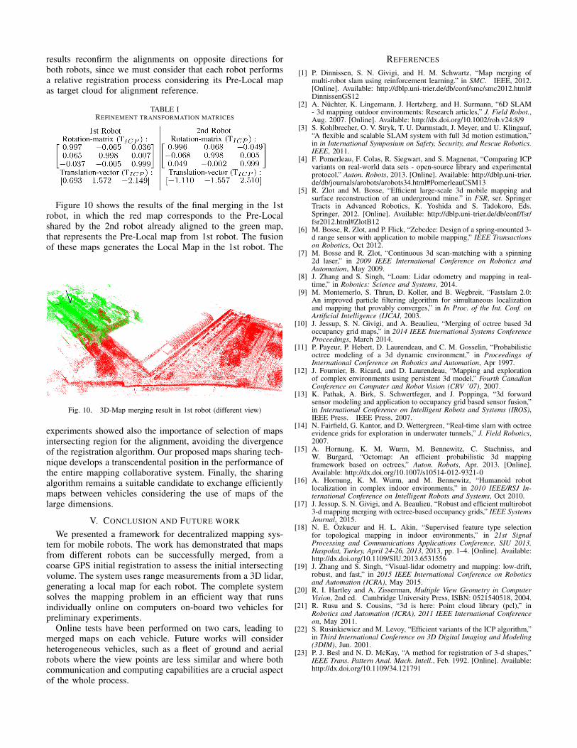
Figure 10 shows the results of the final merging in the 1strobot, in which the red map corresponds to the Pre-Localshared by the 2nd robot already aligned to the green map,that represents the Pre-Local map from 1st robot. The fusionof these maps generates the Local Map in the 1st robot. The

Fig. 10. 3D-Map merging result in 1st robot (different view)

experiments showed also the importance of selection of mapsintersecting region for the alignment, avoiding the divergenceof the registration algorithm. Our proposed maps sharing tech-nique develops a transcendental position in the performance ofthe entire mapping collaborative system. Finally, the sharingalgorithm remains a suitable candidate to exchange efficientlymaps between vehicles considering the use of maps of thelarge dimensions.

V. CONCLUSION AND FUTURE WORK

We presented a framework for decentralized mapping sys-tem for mobile robots. The work has demonstrated that mapsfrom different robots can be successfully merged, from acoarse GPS initial registration to assess the initial intersectingvolume. The system uses range measurements from a 3D lidar,generating a local map for each robot. The complete systemsolves the mapping problem in an efficient way that runsindividually online on computers on-board two vehicles forpreliminary experiments.

Online tests have been performed on two cars, leading tomerged maps on each vehicle. Future works will considerheterogeneous vehicles, such as a fleet of ground and aerialrobots where the view points are less similar and where bothcommunication and computing capabilities are a crucial aspectof the whole process.

REFERENCES

[1] P. Dinnissen, S. N. Givigi, and H. M. Schwartz, “Map merging ofmulti-robot slam using reinforcement learning.” in SMC. IEEE, 2012.[Online]. Available: http://dblp.uni-trier.de/db/conf/smc/smc2012.html#DinnissenGS12

[2] A. Nuchter, K. Lingemann, J. Hertzberg, and H. Surmann, “6D SLAM- 3d mapping outdoor environments: Research articles,” J. Field Robot.,Aug. 2007. [Online]. Available: http://dx.doi.org/10.1002/rob.v24:8/9

[3] S. Kohlbrecher, O. V. Stryk, T. U. Darmstadt, J. Meyer, and U. Klingauf,“A flexible and scalable SLAM system with full 3d motion estimation,”in in International Symposium on Safety, Security, and Rescue Robotics.IEEE, 2011.

[4] F. Pomerleau, F. Colas, R. Siegwart, and S. Magnenat, “Comparing ICPvariants on real-world data sets - open-source library and experimentalprotocol.” Auton. Robots, 2013. [Online]. Available: http://dblp.uni-trier.de/db/journals/arobots/arobots34.html#PomerleauCSM13

[5] R. Zlot and M. Bosse, “Efficient large-scale 3d mobile mapping andsurface reconstruction of an underground mine.” in FSR, ser. SpringerTracts in Advanced Robotics, K. Yoshida and S. Tadokoro, Eds.Springer, 2012. [Online]. Available: http://dblp.uni-trier.de/db/conf/fsr/fsr2012.html#ZlotB12

[6] M. Bosse, R. Zlot, and P. Flick, “Zebedee: Design of a spring-mounted 3-d range sensor with application to mobile mapping,” IEEE Transactionson Robotics, Oct 2012.

[7] M. Bosse and R. Zlot, “Continuous 3d scan-matching with a spinning2d laser,” in 2009 IEEE International Conference on Robotics andAutomation, May 2009.

[8] J. Zhang and S. Singh, “Loam: Lidar odometry and mapping in real-time,” in Robotics: Science and Systems, 2014.

[9] M. Montemerlo, S. Thrun, D. Koller, and B. Wegbreit, “Fastslam 2.0:An improved particle filtering algorithm for simultaneous localizationand mapping that provably converges,” in In Proc. of the Int. Conf. onArtificial Intelligence (IJCAI, 2003.

[10] J. Jessup, S. N. Givigi, and A. Beaulieu, “Merging of octree based 3doccupancy grid maps,” in 2014 IEEE International Systems ConferenceProceedings, March 2014.

[11] P. Payeur, P. Hebert, D. Laurendeau, and C. M. Gosselin, “Probabilisticoctree modeling of a 3d dynamic environment,” in Proceedings ofInternational Conference on Robotics and Automation, Apr 1997.

[12] J. Fournier, B. Ricard, and D. Laurendeau, “Mapping and explorationof complex environments using persistent 3d model,” Fourth CanadianConference on Computer and Robot Vision (CRV ’07), 2007.

[13] K. Pathak, A. Birk, S. Schwertfeger, and J. Poppinga, “3d forwardsensor modeling and application to occupancy grid based sensor fusion,”in International Conference on Intelligent Robots and Systems (IROS),IEEE Press. IEEE Press, 2007.

[14] N. Fairfield, G. Kantor, and D. Wettergreen, “Real-time slam with octreeevidence grids for exploration in underwater tunnels,” J. Field Robotics,2007.

[15] A. Hornung, K. M. Wurm, M. Bennewitz, C. Stachniss, andW. Burgard, “Octomap: An efficient probabilistic 3d mappingframework based on octrees,” Auton. Robots, Apr. 2013. [Online].Available: http://dx.doi.org/10.1007/s10514-012-9321-0

[16] A. Hornung, K. M. Wurm, and M. Bennewitz, “Humanoid robotlocalization in complex indoor environments,” in 2010 IEEE/RSJ In-ternational Conference on Intelligent Robots and Systems, Oct 2010.

[17] J. Jessup, S. N. Givigi, and A. Beaulieu, “Robust and efficient multirobot3-d mapping merging with octree-based occupancy grids,” IEEE SystemsJournal, 2015.

[18] N. E. Ozkucur and H. L. Akin, “Supervised feature type selectionfor topological mapping in indoor environments,” in 21st SignalProcessing and Communications Applications Conference, SIU 2013,Haspolat, Turkey, April 24-26, 2013, 2013, pp. 1–4. [Online]. Available:http://dx.doi.org/10.1109/SIU.2013.6531556

[19] J. Zhang and S. Singh, “Visual-lidar odometry and mapping: low-drift,robust, and fast,” in 2015 IEEE International Conference on Roboticsand Automation (ICRA), May 2015.

[20] R. I. Hartley and A. Zisserman, Multiple View Geometry in ComputerVision, 2nd ed. Cambridge University Press, ISBN: 0521540518, 2004.

[21] R. Rusu and S. Cousins, “3d is here: Point cloud library (pcl),” inRobotics and Automation (ICRA), 2011 IEEE International Conferenceon, May 2011.

[22] S. Rusinkiewicz and M. Levoy, “Efficient variants of the ICP algorithm,”in Third International Conference on 3D Digital Imaging and Modeling(3DIM), Jun. 2001.

[23] P. J. Besl and N. D. McKay, “A method for registration of 3-d shapes,”IEEE Trans. Pattern Anal. Mach. Intell., Feb. 1992. [Online]. Available:http://dx.doi.org/10.1109/34.121791