Montréal

Juillet 2013

© 2013 Marine Carrasco, Guy Tchuente. Tous droits réservés. All rights reserved. Reproduction partielle

permise avec citation du document source, incluant la notice ©.

Short sections may be quoted without explicit permission, if full credit, including © notice, is given to the source.

Série Scientifique

Scientific Series

2013s-21

Efficient estimation with many weak

instruments using regularization techniques

Marine Carrasco, Guy Tchuente

CIRANO

Le CIRANO est un organisme sans but lucratif constitué en vertu de la Loi des compagnies du Québec. Le financement de

son infrastructure et de ses activités de recherche provient des cotisations de ses organisations-membres, d’une subvention

d’infrastructure du Ministère du Développement économique et régional et de la Recherche, de même que des subventions et

mandats obtenus par ses équipes de recherche.

CIRANO is a private non-profit organization incorporated under the Québec Companies Act. Its infrastructure and research

activities are funded through fees paid by member organizations, an infrastructure grant from the Ministère du

Développement économique et régional et de la Recherche, and grants and research mandates obtained by its research

teams.

Les partenaires du CIRANO

Partenaire majeur

Ministère de l'Enseignement supérieur, de la Recherche, de la Science et de la Technologie

Partenaires corporatifs

Autorité des marchés financiers

Banque de développement du Canada

Banque du Canada

Banque Laurentienne du Canada

Banque Nationale du Canada

Banque Scotia

Bell Canada

BMO Groupe financier

Caisse de dépôt et placement du Québec

Fédération des caisses Desjardins du Québec

Financière Sun Life, Québec

Gaz Métro

Hydro-Québec

Industrie Canada

Investissements PSP

Ministère des Finances et de l’Économie

Power Corporation du Canada

Rio Tinto Alcan

State Street Global Advisors

Transat A.T.

Ville de Montréal

Partenaires universitaires

École Polytechnique de Montréal

École de technologie supérieure (ÉTS)

HEC Montréal

Institut national de la recherche scientifique (INRS)

McGill University

Université Concordia

Université de Montréal

Université de Sherbrooke

Université du Québec

Université du Québec à Montréal

Université Laval

Le CIRANO collabore avec de nombreux centres et chaires de recherche universitaires dont on peut consulter la liste sur son

site web.

ISSN 1198-8177

Les cahiers de la série scientifique (CS) visent à rendre accessibles des résultats de recherche effectuée au CIRANO afin

de susciter échanges et commentaires. Ces cahiers sont écrits dans le style des publications scientifiques. Les idées et les

opinions émises sont sous l’unique responsabilité des auteurs et ne représentent pas nécessairement les positions du

CIRANO ou de ses partenaires.

This paper presents research carried out at CIRANO and aims at encouraging discussion and comment. The observations

and viewpoints expressed are the sole responsibility of the authors. They do not necessarily represent positions of

CIRANO or its partners.

Partenaire financier

Efficient estimation with many weak instruments

using regularization techniques *

Marine Carrasco †, Guy Tchuente

‡

Résumé / Abstract

The problem of weak instruments is due to a very small concentration parameter. To boost the

concentration parameter, we propose to increase the number of instruments to a large number or even

up to a continuum. However, in finite samples, the inclusion of an excessive number of moments may

be harmful. To address this issue, we use regularization techniques as in Carrasco (2012) and Carrasco

and Tchuente (2013). We show that normalized regularized 2SLS and LIML are consistent and

asymptotically normally distributed. Moreover, their asymptotic variances reach the semiparametric

efficiency bound unlike most competing estimators. Our simulations show that the leading regularized

estimators (LF and T of LIML) work very well (is nearly median unbiased) even in the case of

relatively weak instruments.

Mots clés/Keywords : Many weak instruments, LIML, 2SLS, regularization methods.

* Carrasco gratefully acknowledges financial support from SSHRC.

† University of Montreal, CIREQ, CIRANO, email: marine.carrasco@umontreal.ca.

‡ University of Montreal, CIREQ, email: guy.tchuente.nguembu@umontreal.ca.

1 Introduction

The problem of weak instruments or weak identi�cation has recently received consid-

erable attention in both theoretical and applied econometrics1. Empirical examples

include Angrist and Krueger (1991) who measure return to schooling, Eichenbaum,

Hansen, and Singleton (1988) who consider consumption asset pricing models. The-

oretical literature on weak instruments includes papers by Staiger and Stock (1997),

Zivot, Startz, and Nelson (1998), Guggenberger and Smith (2005), Chao and Swanson

(2005), Han and Phillips (2006), Hansen, Hausman, and Newey (2008), and Newey and

Windmeijer (2009) among others2. Staiger and Stock (1997) proposed an asymptotic

framework with local-to-zero parametrization of the coe¢ cients of the instruments in

the �rst-stage regression. They show that with the number of instruments �xed, the

two-stage least squares (2SLS) and limited information maximum likelihood (LIML)

estimators are not consistent and converge to nonstandard distributions. Subsequent

work focused on situations where the number of instruments is large, using an asymp-

totic framework that lets the number of instruments go to in�nity as a function of

sample size. In these settings, the use of many moments can improve estimator ac-

curacy. Unfortunately, usual Gaussian asymptotic approximation can be poor and IV

estimators can be biased.

Carrasco (2012) and Carrasco and Tchuente (2013) proposed respectively regular-

ized versions of 2SLS and LIML estimators for many strong instruments. The regu-

larization permits to address the singularity of the covariance matrix resulting from

many instruments. These papers use three regularization methods borrowed from in-

verse problem literature. The �rst estimator is based on Tikhonov (ridge) regulariza-

tion, the second estimator is based on an iterative method called Landweber-Fridman

(LF), the third estimator is based on the principal components associated with the

largest eigenvalues. We extend these previous works to allow for the presence of a

1Hahn and Hausman (2003) de�ne weak instruments, by two features: (i) two-stage least squares (2SLS)analysis is badly biased toward the ordinary least-squares (OLS) estimate, and alternative unbiased esti-mators such as limited-information maximum likelihood (LIML) may not solve the problem; and (ii) thestandard (�rst-order) asymptotic distribution does not give an accurate framework for inference. Weak in-strument may also be an important cause of the �nding that the often-used test of over identifying restrictions(OID test) rejects too often.

2Section 4 discusses related literature in more details.

2

large number of weak instruments or weak identi�cation. We consider a linear model

with homoskedastic error and allow for weak identi�cation as in Hansen, Hausman,

and Newey (2008) and Newey and Windmeijer (2009). This speci�cation helps us to

have di¤erent types of weak instruments sequences, including the many instruments

sequence of Bekker (1994) and the many weak instruments sequence of Chao and Swan-

son (2005). We impose no condition on the number of moment conditions since our

framework allows for an in�nite countable or even a continuum of instruments. The ad-

vantage of regularization is that all available moments can be used without discarding

any a priori. We show that regularized 2SLS and LIML are consistent in the presence

of many weak instruments. If properly normalized, the regularized 2SLS and LIML

are asymptotically normal and reach the semiparametric e¢ ciency bounds. There-

fore, their asymptotic variance is smaller than that of Hansen, Hausman, and Newey

(2008) and Newey and Windmeijer (2009). All these methods involve a regularization

parameter, which is the counterpart of the smoothing parameter that appears in the

nonparametric literature. A data driven method was developed in Carrasco (2012)

and Carrasco and Tchuente (2013) to select the best regularization parameter when

the instruments are strong. We use these methods in our simulations for selecting the

regularization parameter when the instruments are weak but we do not prove that

these methods are valid in this case.

A Monte-carlo experiment shows that the leading regularized estimators (LF and

T LIML) perform very well (are nearly median unbiased) even in the case of weak

instruments.

The paper is organized as follows. Section 2 introduces four regularization methods

we consider and the associated estimators. Section 3 derives the asymptotic properties

of the estimators. Section 4 discusses e¢ ciency and related results. Section 5 presents

Monte Carlo experiments. Section 6 concludes. The proofs are collected in Appendix.

3

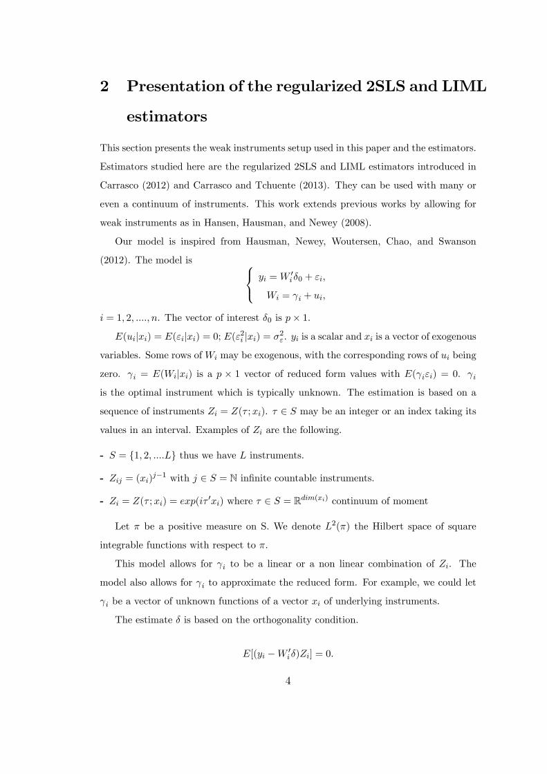
2 Presentation of the regularized 2SLS and LIML

estimators

This section presents the weak instruments setup used in this paper and the estimators.

Estimators studied here are the regularized 2SLS and LIML estimators introduced in

Carrasco (2012) and Carrasco and Tchuente (2013). They can be used with many or

even a continuum of instruments. This work extends previous works by allowing for

weak instruments as in Hansen, Hausman, and Newey (2008).

Our model is inspired from Hausman, Newey, Woutersen, Chao, and Swanson

(2012). The model is 8<: yi =W 0i�0 + "i;

Wi = i + ui;

i = 1; 2; ::::; n. The vector of interest �0 is p� 1.

E(uijxi) = E("ijxi) = 0; E("2i jxi) = �2". yi is a scalar and xi is a vector of exogenous

variables. Some rows ofWi may be exogenous, with the corresponding rows of ui being

zero. i = E(Wijxi) is a p � 1 vector of reduced form values with E( i"i) = 0. i

is the optimal instrument which is typically unknown. The estimation is based on a

sequence of instruments Zi = Z(� ;xi). � 2 S may be an integer or an index taking its

values in an interval. Examples of Zi are the following.

- S = f1; 2; ::::Lg thus we have L instruments.

- Zij = (xi)j�1 with j 2 S = N in�nite countable instruments.

- Zi = Z(� ;xi) = exp(i� 0xi) where � 2 S = Rdim(xi) continuum of moment

Let � be a positive measure on S. We denote L2(�) the Hilbert space of square

integrable functions with respect to �.

This model allows for i to be a linear or a non linear combination of Zi. The

model also allows for i to approximate the reduced form. For example, we could let

i be a vector of unknown functions of a vector xi of underlying instruments.

The estimate � is based on the orthogonality condition.

E[(yi �W 0i�)Zi] = 0:

4

The extension of the generalized method of moments described in Carrasco and Florens

(2000), Carrasco and Florens (2012), and Carrasco (2012) gives the regularized 2SLS.

Let W =

0BBBBBBBBB@

W 01

W 02

:

:

W 0n

1CCCCCCCCCAn� p and u =

0BBBBBBBBB@

u01

u02

:

:

u0n

1CCCCCCCCCAn� p.

We de�ne the covariance operator K of the instruments as

K : L2(�) ! L2(�)

(Kg)(�1) =

ZE(Z(�1;xi)Z(�2;xi))g(�2)�(�2)d�2

where Z(�2;xi) denotes the complex conjugate of Z(�2;xi).

K is assumed to be a Hilbert-Schmidt operator. Let �j an �j ; j = 1; 2; ::: be re-

spectively, the eigenvalues (ranked in decreasing order) and orthonormal eigenfunctions

of K. K can be estimated by Kn de�ned as:

Kn : L2(�) ! L2(�)

(Kng)(�1) =

Z1

n

nXi=1

Z(�1;xi)Z(�2;xi)g(�2)�(�2)d�2:

If the number of moment conditions is in�nite then the inverse of Kn needs to be

regularized because it is not continuous. By de�nition (see Kress, 1999, page 269), a

regularized inverse of an operator K is

R� : L2(�) ! L2(�)

such that lim�!0

R�K' = ', 8' 2 L2(�):

Three di¤erent types of regularization schemes are considered: Tikhonov (T),

Landwerber Fridman (LF), Spectral cut-o¤ (SC) or Principal Components (PC). They

are de�ned as follows:

5

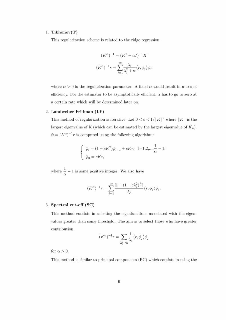
1. Tikhonov(T)

This regularization scheme is related to the ridge regression.

(K�)�1 = (K2 + �I)�1K

(K�)�1r =1Xj=1

�j

�2j + �

r; �j

��j

where � > 0 is the regularization parameter. A �xed � would result in a loss of

e¢ ciency. For the estimator to be asymptotically e¢ cient, � has to go to zero at

a certain rate which will be determined later on.

2. Landweber Fridman (LF)

This method of regularization is iterative. Let 0 < c < 1=kKk2 where kKk is the

largest eigenvalue of K (which can be estimated by the largest eigenvalue of Kn).

' = (K�)�1r is computed using the following algorithm:

8<: 'l = (1� cK2)'l�1 + cKr; l=1,2,...,1

�� 1;

'0 = cKr;

where1

�� 1 is some positive integer. We also have

(K�)�1r =1Xj=1

[1� (1� c�2j )1� ]

�j

r; �j

��j :

3. Spectral cut-o¤ (SC)

This method consists in selecting the eigenfunctions associated with the eigen-

values greater than some threshold. The aim is to select those who have greater

contribution.

(K�)�1r =X�2j��

1

�j

r; �j

��j

for � > 0:

This method is similar to principal components (PC) which consists in using the

6

�rst eigenfunctions:

(K�)�1r =

1=�Xj=1

1

�j

r; �j

��j

where1

�is some positive integer. It is equivalent to projecting on the �rst

principal components of W . Interestingly, this approach is used in factor models

where Wi is assumed to depend on a �nite number of factors (see Bai and Ng

(2002), Stock and Watson (2002)) As the estimators based on PC and SC are

identical, we will use PC and SC interchangeably.

These regularized inverses can be rewritten in common notation as:

(K�)�1r =1Xj=1

q(�; �2j )

�j

r; �j

��j

where for T: q(�; �2j ) =�2j

�2j + �;

for LF: q(�; �2j ) = [1� (1� c�2j )1=�],

for SC: q(�; �2j ) = I(�2j � �), for PC q(�; �2j ) = I(j � 1=�).

In order to compute the inverse of Kn we have to choose the regularization para-

meter �. Let (K�n )�1 be the regularized inverse of Kn and P� a n� n matrix de�ned

as in Carrasco (2012) by P� = T (K�n )�1T � where

T : L2(�) ! Rn

Tg =

0BBBBBBBBB@

Z1; g

�Z2; g

�:

:Zn; g

�

1CCCCCCCCCA

and

T � : Rn ! L2(�)

7

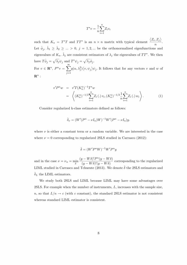
T �v =1

n

nXi=1

Zivi

such that Kn = T �T and TT � is an n � n matrix with typical element

Zi; Zj

�n

.

Let �j , �1 � �2 � ::: > 0, j = 1; 2; ::: be the orthonormalized eigenfunctions and

eigenvalues of Kn: �j are consistent estimators of �j the eigenvalues of TT �. We then

have T �j =p�j j and T

� j =p�j�j .

For v 2 Rn, P�v =1Xj=1

q(�; �2j )v; j

� j : It follows that for any vectors v and w of

Rn :

v0P�w = v0T (K�n )�1T �w

=

*(K�

n )�1=2

nXi=1

Zi (:) vi; (K�n )�1=2 1

n

nXi=1

Zi (:)wi

+: (1)

Consider regularized k-class estimators de�ned as follows:

�� = (W0(P� � �In)W )�1W 0(P� � �In)y:

where � is either a constant term or a random variable. We are interested in the case

where � = 0 corresponding to regularized 2SLS studied in Carrasco (2012):

� = (W 0P�W )�1W 0P�y

and in the case � = �� = min�

(y �W�)0P�(y �W�)

(y �W�)0(y �W�)corresponding to the regularized

LIML studied in Carrasco and Tchuente (2013). We denote � the 2SLS estimators and

�L the LIML estimators.

We study both 2SLS and LIML because LIML may have some advantages over

2SLS. For example when the number of instruments, L, increases with the sample size,

n, so that L=n ! c (with c constant), the standard 2SLS estimator is not consistent

whereas standard LIML estimator is consistent.

8

3 Asymptotic properties

In Carrasco (2012) and Carrasco and Tchuente (2013), modi�ed IV estimators based on

di¤erent regularization schemes were proposed. These estimators improved the small

sample properties of IV estimators when the number of instruments is very large or

in�nite. The focus was on strong instruments. They found that regularized 2SLS and

LIML estimators are asymptotically normal and attain the semiparametric e¢ ciency

bound. We extend Carrasco (2012) and Carrasco and Tchuente (2013) results to the

case of weak instruments.

Assumption 1:

i) There exists a p � p matrix Sn = ~Sndiag(�1n; :::; �pn) such that ~Sn is bounded,

the smallest eigenvalue of ~Sn ~S0n is bounded away from zero; for each j, either

�jn =pn (strong identi�cation) or �jn=

pn! 0 (weak identi�cation),

�n = min1�j�p

�jn !1 and �! 0.

ii) There exists a function fi = f(xi) such that i = Snfi=pn and �nS

�1n ! S0:

nXi=1

kfik4 =n2 ! 0,nXi=1

fif0i=n is bounded and uniformly nonsingular.

These conditions allow for many weak instruments. If �jn =pn this leads to

asymptotic theory like in Kunitomo (1980), Morimune (1983), and Bekker (1994),

but here we use regularization parameter instead of having an increasing sequence of

instruments. For �2n growing slower than n the convergence rate will be slower thatpn,

leading to an asymptotic approximation like that of Chao and Swanson (2005). This is

the case where we have many instruments without strong identi�cation. Assumption

1 also allows for some components of the reduced form to give only weak identi�cation

(corresponding to �jn=pn ! 0 which allows the concentration parameter to grow

slower thanpn), and other components (corresponding to �jn =

pn) to give strong

identi�cation for some coe¢ cients of the reduced form. In particular, this condition

allows for �xed constant coe¢ cients in the reduced form. This speci�cation of weak

instruments can also be viewed as a generalization of Chao and Swanson (2007). This

speci�cation of weak identi�cation is di¤erent of Antoine and Lavergne (2012) whose

identi�cation strength is directly de�ned through the conditional moments that �atten

9

as the sample size increases. To illustrate Assumption 1 let us consider the following

example.

Example 1: Assume that p = 2, ~Sn =

0@ 1 0

�21 1

1A, and �jn =8<:pn; j = 1

�n; j = 2.

Then for f(xi) = (f 01i; f02i)0 the reduced form is

i =

0B@ f1i

�21f1i +�npnf2i

1CA :

We also have

�nS�1n ! S0 =

0@ 0 0

��21 1

1A :

Proposition 1. (Asymptotic properties of regularized 2SLS with many weak instru-

ments)

Assume fyi;Wi;xig are iid, E("2i jX) = �2", K is compact, � goes to zero and n

goes to in�nity. Moreover, a belongs to the closure of the linear span of fZ(:;x)g

for a = 1; :::; p; E(Z(:; xi)fia) belong to the range of K and Assumption 1 is satis�ed.

Then, the T, LF, and SC estimators of 2SLS satisfy:

1. Consistency: S0n(� � �0)=�n ! 0 in probability as n, n�12 and �n go to in�nity.

This implies (� � �0)! 0.

2. Asymptotic normality: moreover, if each element of E(Z(:;xi)Wi) belongs to the

range of K, then

S0n(� � �0)d! N

�0; �2"

�E(fif

0i)��1�

as n, n� and �n go to in�nity; where E(fif0i) is the p� p matrix.

Proof In Appendix.

This result shows that the three estimators have the same asymptotic distribution.

Instead of restricting the number of instruments, we have a regularization parameter

which goes to zero. This insures us that all available and valid instruments are used

in an e¢ cient way even if there are weak. To obtain consistency, the condition on � is

n�12 go in�nity, whereas for the asymptotic normality, we need n� go to in�nity. This

means that � is allowed to go to zero at a slower rate. However this rate does not

depend on the weakness of the instruments.

10

Interestingly, our regularized 2SLS estimators reach the semiparametric e¢ ciency

bound. This result will be further discussed in Section 4.

We are now going derive the asymptotic properties of the regularized LIML with

many weak instruments.

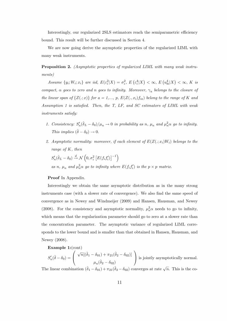
Proposition 2. (Asymptotic properties of regularized LIML with many weak instru-

ments)

Assume fyi;Wi;xig are iid, E("2i jX) = �2", E�"4i jX

�< 1; E

�u4bijX

�< 1; K is

compact, � goes to zero and n goes to in�nity. Moreover, a belongs to the closure of

the linear span of fZ(:;x)g for a = 1,..., p, E(Z(:; xi)fia) belong to the range of K and

Assumption 1 is satis�ed. Then, the T, LF, and SC estimators of LIML with weak

instruments satisfy:

1. Consistency: S0n(�L � �0)=�n ! 0 in probability as n, �n and �2n� go to in�nity.

This implies (� � �0)! 0.

2. Asymptotic normality: moreover, if each element of E(Z(:;xi)Wi) belongs to the

range of K, then

S0n(�L � �0)d! N

�0; �2"

�E(fif

0i)��1�

as n, �n and �2n� go to in�nity where E(fif

0i) is the p� p matrix.

Proof In Appendix.

Interestingly we obtain the same asymptotic distribution as in the many strong

instruments case (with a slower rate of convergence). We also �nd the same speed of

convergence as in Newey and Windmeijer (2009) and Hansen, Hausman, and Newey

(2008). For the consistency and asymptotic normality, �2n� needs to go to in�nity,

which means that the regularization parameter should go to zero at a slower rate than

the concentration parameter. The asymptotic variance of regularized LIML corre-

sponds to the lower bound and is smaller than that obtained in Hansen, Hausman, and

Newey (2008).

Example 1:(cont)

S0n(�� �0) =

0@ pn[(�1 � �01) + �21(�2 � �02)]

�n(�2 � �02)

1A is jointly asymptotically normal.

The linear combination (�1� �01)+�21(�2� �02) converges at ratepn. This is the co-

11

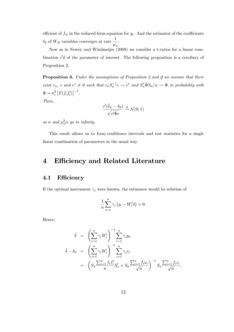
e¢ cient of fi1 in the reduced form equation for yi. And the estimator of the coe¢ cients

�2 of Wi2 variables converges at rate1

�n.

Now as in Newey and Windmeijer (2009) we consider a t-ratios for a linear com-

bination c0� of the parameter of interest. The following proposition is a corollary of

Proposition 2.

Proposition 3. Under the assumptions of Proposition 2 and if we assume that there

exist rn, c and c� 6= 0 such that rnS�1n c ! c� and S0n�Sn=n ! � in probability with

� = �2"�E(fif

0i)��1.

Then,c0(�L � �0)p

c0�c

d! N (0; 1)

as n and �2n� go to in�nity.

This result allows us to form con�dence intervals and test statistics for a single

linear combination of parameters in the usual way.

4 E¢ ciency and Related Literature

4.1 E¢ ciency

If the optimal instrument i were known, the estimator would be solution of

1

n

nXi=1

i�yi �W 0

i��= 0:

Hence,

� =

nXi=1

iW0i

!�1 nXi=1

iyi;

� � �0 =

nXi=1

iW0i

!�1 nXi=1

i"i

=

�Sn

Pni=1 fif

0i

nS0n + Sn

Pni=1 fiuipn

��1Sn

Pni=1 fi"ipn

;

12

Sn

�� � �0

�=

�Pni=1 fif

0i

n+

Pni=1 fiuipn

S0�1n

��1 Pni=1 fi"ipn

d! N�0; �2"

�E�fif

0i

���1�:

So the lowest asymptotic variance that can be obtained is �2"�E�fif

0i

���1: We will

refer to this as the semiparametric e¢ ciency bound.

Now, if the i is unknown but estimated by a consistent nonparametric estimator

i. The resulting estimator

� =

nXi=1

iW0i

!�1 nXi=1

iyi;

will satisfy Sn�� � �0

�d! N

�0; �2"

�E�fif

0i

���1� regardless of the convergence rate of i. This can be proved using the same arguments as in Newey (1990).

In Carrasco (2012, Section 2.4), it was shown that the regularized 2SLS estimator

coincides with a 2SLS estimator that uses a speci�c nonparametric estimator of i:

This explains why for the regularized 2SLS estimator, the conditions on � are not

related to �n: On the contrary, LIML can not written as such a 2SLS estimator. This

may explain why in the case of LIML, the rate of convergence of � depends on how

weak the instruments are.

4.2 Related Literature

In the literature on many weak instruments the asymptotic behavior of estimator de-

pends on the relation between the number of moment conditions and sample size. For

the CUE, the number of moments L and the sample size n needs to satisfy L2=n! 0 to

have consistency. Asymptotic normality, requires L3=n! 0. Under homoskedasticity,

Stock and Yogo (2005) require L2=n ! 0. Hansen, Hausman, and Newey (2008) al-

lowed L to grow at the same rate as n, but restricted L to grow slower than the square

of the concentration parameter, for the consistency of LIML and FULL. Andrews and

Stock (2006) require L3=n! 0 when normality is not imposed.

Caner and Yildiz (2012) in a recent work consider a Continuous Updating Estima-

tor (CUE) with many weak moments under nearly singular design. They show that the

13

nearly singular design a¤ects the form of asymptotic covariance matrix of the estimator

compared to that of Newey and Windmeijer (2009). Our work is also related to Haus-

man, Lewis, Menzel, and Newey (2011) who propose the Regularized CUE (RCUE)

as a solution in presence of many weak instruments. The RCUE solves a modi�cation

of the �rst-order conditions for the CUE estimator and is shown to be asymptotically

equivalent to CUE under many weak moments asymptotics.

Belloni, Chen, Chernozhukov, and Hansen (2012) propose to use an alternative

regularization named lasso in the IV context. This regularization imposes a l1 type

penalty on the �rst stage coe¢ cient. Assuming that the �rst stage equation is approxi-

mately sparse, they show that the postlasso estimator reaches the asymptotic e¢ ciency

bound.

Just as 2SLS is not consistent if L is too large relative to n, LIML estimator is

not feasible if L > N because the matrix Z 0Z is not invertible. Therefore, some form

of regularization needs to be implemented to obtain consistent estimators when the

number of instruments is really large. Regularization has also the advantage to deliver

an asymptotically e¢ cient estimator.

Table 1 gives an overview of the assumptions used in the main papers on many

weak instruments.

Table 1: Comparison of di¤erent IV asymptoticsNumber of instruments Extra assumptions

Conventional Fixed LPhillips (1989) Fixed L, Cov(W;x) = 0Staiger and Stock (1997) Fixed L, Cov(W;x) = O(n�1=2)Bekker (1994) L=n! c < 1; �2n = O(n)

Han and Phillips (2006) L!1 andL

ncn! c

cn �n constant or zero

Chao and Swanson (2005)L

�2n! 0 or

L1=2

�2n! 0

Hansen et al. (2008) (I)L

�2nbounded or (II)

L

�2n!1

Xziz

0i=n nonsingular

Newey and Windmeijer (2009) L!1 andL

�2nbounded

Carrasco (2012) No condition on L, possibly continuum Compactness ofstrong instruments covariance matrix

Belloni et al. (2012) log(L) = o(n1=3); Approximately sparsestrong instruments �rst stage equation

14

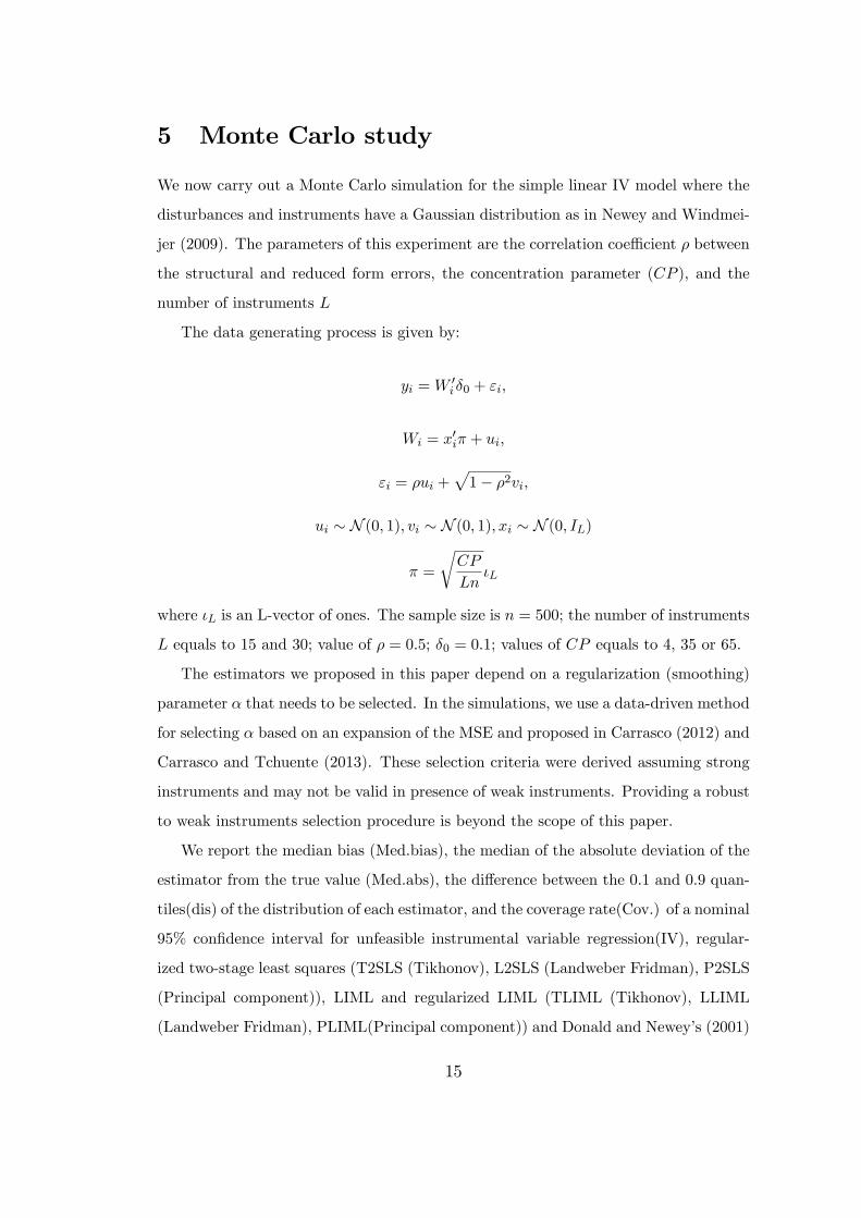
5 Monte Carlo study

We now carry out a Monte Carlo simulation for the simple linear IV model where the

disturbances and instruments have a Gaussian distribution as in Newey and Windmei-

jer (2009). The parameters of this experiment are the correlation coe¢ cient � between

the structural and reduced form errors, the concentration parameter (CP ), and the

number of instruments L

The data generating process is given by:

yi =W 0i�0 + "i;

Wi = x0i� + ui;

"i = �ui +p1� �2vi;

ui � N (0; 1); vi � N (0; 1); xi � N (0; IL)

� =

rCP

Ln�L

where �L is an L-vector of ones. The sample size is n = 500; the number of instruments

L equals to 15 and 30; value of � = 0:5; �0 = 0:1; values of CP equals to 4, 35 or 65.

The estimators we proposed in this paper depend on a regularization (smoothing)

parameter � that needs to be selected. In the simulations, we use a data-driven method

for selecting � based on an expansion of the MSE and proposed in Carrasco (2012) and

Carrasco and Tchuente (2013). These selection criteria were derived assuming strong

instruments and may not be valid in presence of weak instruments. Providing a robust

to weak instruments selection procedure is beyond the scope of this paper.

We report the median bias (Med.bias), the median of the absolute deviation of the

estimator from the true value (Med.abs), the di¤erence between the 0.1 and 0.9 quan-

tiles(dis) of the distribution of each estimator, and the coverage rate(Cov.) of a nominal

95% con�dence interval for unfeasible instrumental variable regression(IV), regular-

ized two-stage least squares (T2SLS (Tikhonov), L2SLS (Landweber Fridman), P2SLS

(Principal component)), LIML and regularized LIML (TLIML (Tikhonov), LLIML

(Landweber Fridman), PLIML(Principal component)) and Donald and Newey�s (2001)

15

2SLS and LIML (D2SLS and DLIML). For con�dence intervals we compute the cover-

age probabilities using the following estimate of asymptotic variance as in Donald and

Newey (2001) and Carrasco (2012).

V (�) =(y �W�)0(y �W�)

n

�W 0W�1

��1W 0W

�W 0W

��1where W = P�W .

Table 2: Simulations results with Cp = 4, 8, 35 and 65 ; n = 500; L = 15 and 30; 1000replications.

T2SLS L2SLS P2SLS D2SLS TLIML LLIML PLIML DLIML IVL=15 Cp=4 Med.b ias 0 .3918 0.3876 0.3567 0.4093 0.1443 0.1378 0.3497 0.3907 0.0212

M ed.abs 0.3925 0.3883 0.5334 0.5633 0.5649 0.5644 0.7021 0.5208 0.3476D isp 0.5590 0.5806 2.6328 2.4639 3.2294 2.9889 3.5783 1.8474 1.5407Cov 0.5040 0.5330 0.7750 0.7750 0.4500 0.4660 0.9010 0.7130 0.9520

Cp=8 Med.b ias 0 .3248 0.3189 0.3036 0.3385 0.0381 0.0383 0.2471 0.2856 0.0031M ed.abs 0.3265 0.3205 0.3917 0.4080 0.3722 0.3698 0.6087 0.3864 0.2506

D isp 0.5044 0.5388 1.5854 1.7167 1.9193 1.9012 3.1534 1.3395 1.0210Cov 0.5630 0.5900 0.7420 0.7380 0.5690 0.5790 0.9240 0.7210 0.9500

Cp=35 Med.b ias 0 .1421 0.1409 0.1584 0.1940 0.0003 0.0013 0.0669 0.0383 0.0012M ed.abs 0.1519 0.1524 0.1938 0.2123 0.1337 0.1357 0.2734 0.1316 0.1214

D isp 0.3426 0.3656 0.4974 0.4297 0.5348 0.5448 1.4268 0.4907 0.4551Cov 0.7680 0.7810 0.7770 0.7430 0.8580 0.8680 0.9340 0.8640 0.9540

Cp=65 Med.b ias 0 .0876 0.0865 0.0953 0.1198 -0 .0010 0.0025 0.0295 0.0061 0.0009M ed.abs 0.1012 0.1051 0.1222 0.1343 0.0927 0.0905 0.1533 0.0920 0.0881

D isp 0.2796 0.2932 0.3359 0.3039 0.3482 0.3505 0.7478 0.3483 0.3240Cov 0.8350 0.8300 0.8340 0.8120 0.9020 0.8960 0.9330 0.8980 0.9550

L=30 Cp=4 Med.b ias 0 .4493 0.4401 0.3622 0.4197 0.2147 0.1825 0.3792 0.4156 0.0280M ed.abs 0.4493 0.4401 0.5737 0.6374 0.6517 0.6559 0.6629 0.5265 0.3822

D isp 0.4037 0.4378 2.8445 3.2928 3.7483 3.6305 2.9905 1.9820 1.5888Cov 0.2010 0.2680 0.7870 0.7780 0.2850 0.3180 0.8860 0.7010 0.9600

Cp=8 Med.b ias 0 .4019 0.3893 0.3260 0.3802 0.0618 0.0800 0.2915 0.3591 -0 .0096M ed.abs 0.4019 0.3893 0.4665 0.5419 0.4413 0.4568 0.5940 0.4513 0.2624

D isp 0.3857 0.4262 2.4101 2.6333 2.4090 2.2558 2.7095 1.4976 1.0184Cov 0.2470 0.3270 0.7530 0.7180 0.3790 0.4010 0.9000 0.6960 0.9540

Cp=35 Med.b ias 0 .2316 0.2174 0.2211 0.2681 0.0028 0.0078 0.1054 0.1243 -0 .0046M ed.abs 0.2316 0.2176 0.2617 0.2912 0.1530 0.1558 0.3991 0.1827 0.1203

D isp 0.2938 0.3195 0.6125 0.6097 0.6115 0.6275 2.0311 0.6385 0.4363Cov 0.4810 0.5580 0.6870 0.6270 0.7190 0.7340 0.9500 0.7180 0.9580

Cp=65 Med.b ias 0 .1586 0.1466 0.1582 0.2026 0.0038 0.0037 0.0558 0.0335 -0 .0032M ed.abs 0.1586 0.1475 0.1868 0.2186 0.1023 0.1027 0.2440 0.1028 0.0883

D isp 0.2545 0.2710 0.4219 0.4517 0.3918 0.3989 1.2399 0.3962 0.3156Cov 0.6120 0.6610 0.7370 0.6750 0.8330 0.8320 0.9410 0.8270 0.9590

Table 2 reports simulation results. We use di¤erent strength (measured by the

concentration parameter) of instruments and number of instruments. We investigate

the case of very weak instruments for example, when CP = 8 and L = 30, the �rst

stage F-statistic equalsCP

L= 0:26.

We observe that

(a) The performances of the regularized estimators increase with the strength of

instruments but decrease with the number of instruments. Providing regularization

parameter selection procedure robust to weak instruments would certainly improve

these results.

16

(b) The bias of regularized LIML is quite a bit smaller than that of regularized

2SLS.

(c) The bias of our regularized estimators are smaller that those of the corresponding

Donald and Newey�s estimators.

(d) LF LIML and T-LIML estimators have very low median bias even in the case

of relatively weak instruments (CP=8).

(e) The coverage of our estimators deteriorates when the instruments are weak.

6 Conclusion

This paper illustrate the usefulness of regularization techniques for estimation in many

weak instruments framework. We derived the properties of the regularized 2SLS and

LIML estimators in the presence of many or a continuum of moments that may be

weak. We show that if well normalized the regularized 2SLS and LIML are consistent

and reach the semiparametric e¢ ciency bound. Our simulations show that the leading

regularized estimators (LF and T of LIML) perform well.

In this work we restricted our investigation to 2SLS and LIML with weak instru-

ments. It would be interesting, for future research to study the behavior of regularized

version of other k-class estimators, such as FULL or B2SLS or other estimators as

GMM or GEL, in presence of many weak instruments. This will help us to have re-

sults that can be compared with those of Newey and Windmeijer (2009) and Hansen,

Hausman, and Newey (2008). Another topic of interest is the use of our regularization

tools to provide version of robust tests for weak instruments as AR, LM, CLR or KLM

tests, that can be used with a large number or a continuum of moment conditions.

17

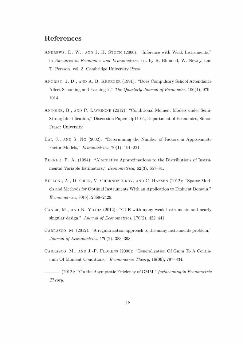
References

Andrews, D. W., and J. H. Stock (2006): �Inference with Weak Instruments,�

in Advances in Economics and Econometrics, ed. by R. Blundell, W. Newey, and

T. Persson, vol. 3. Cambridge University Press.

Angrist, J. D., and A. B. Krueger (1991): �Does Compulsory School Attendance

A¤ect Schooling and Earnings?,�The Quarterly Journal of Economics, 106(4), 979�

1014.

Antoine, B., and P. Lavergne (2012): �Conditional Moment Models under Semi-

Strong Identi�cation,�Discussion Papers dp11-04, Department of Economics, Simon

Fraser University.

Bai, J., and S. Ng (2002): �Determining the Number of Factors in Approximate

Factor Models,�Econometrica, 70(1), 191�221.

Bekker, P. A. (1994): �Alternative Approximations to the Distributions of Instru-

mental Variable Estimators,�Econometrica, 62(3), 657�81.

Belloni, A., D. Chen, V. Chernozhukov, and C. Hansen (2012): �Sparse Mod-

els and Methods for Optimal Instruments With an Application to Eminent Domain,�

Econometrica, 80(6), 2369�2429.

Caner, M., and N. Yildiz (2012): �CUE with many weak instruments and nearly

singular design,�Journal of Econometrics, 170(2), 422�441.

Carrasco, M. (2012): �A regularization approach to the many instruments problem,�

Journal of Econometrics, 170(2), 383�398.

Carrasco, M., and J.-P. Florens (2000): �Generalization Of Gmm To A Contin-

uum Of Moment Conditions,�Econometric Theory, 16(06), 797�834.

(2012): �On the Asymptotic E¢ ciency of GMM,�forthcoming in Econometric

Theory.

18

Carrasco, M., and G. Tchuente (2013): �Regularized LIML for many instru-

ments,�Discussion paper, University of Montreal.

Chao, J. C., and N. R. Swanson (2005): �Consistent Estimation with a Large

Number of Weak Instruments,�Econometrica, 73(5), 1673�1692.

(2007): �Alternative approximations of the bias and MSE of the IV esti-

mator under weak identi�cation with an application to bias correction,�Journal of

Econometrics, 137(2), 515�555.

Eichenbaum, M. S., L. P. Hansen, and K. J. Singleton (1988): �A Time Series

Analysis of Representative Agent Models of Consumption and Leisure Choice under

Uncertainty,�The Quarterly Journal of Economics, 103(1), 51�78.

Guggenberger, P., and R. J. Smith (2005): �Generalized Empirical Likelihood

Estimators And Tests Under Partial, Weak, And Strong Identi�cation,�Econometric

Theory, 21(04), 667�709.

Hahn, J., and J. Hausman (2003): �Weak Instruments: Diagnosis and Cures in

Empirical Econometrics,�American Economic Review, 93(2), 118�125.

Han, C., and P. C. B. Phillips (2006): �GMM with Many Moment Conditions,�

Econometrica, 74(1), 147�192.

Hansen, C., J. Hausman, and W. Newey (2008): �Estimation With Many Instru-

mental Variables,�Journal of Business & Economic Statistics, 26, 398�422.

Hausman, J., R. Lewis, K. Menzel, and W. Newey (2011): �Properties of the

CUE estimator and a modi�cation with moments,�Journal of Econometrics, 165(1),

45 �57, Moment Restriction-Based Econometric Methods.

Hausman, J. A., W. K. Newey, T. Woutersen, J. C. Chao, and N. R. Swan-

son (2012): �Instrumental variable estimation with heteroskedasticity and many

instruments,�Quantitative Economics, 3(2), 211�255.

19

Kunitomo, N. (1980): �Asymptotic Expansions of the Distributions of Estimators

in a Linear Functional Relationship and Simultaneous Equations,� Journal of the

American Statistical Association, 75(371), 693�700.

Morimune, K. (1983): �Approximate Distributions of k-Class Estimators When the

Degree of Overidenti�ability Is Large Compared with the Sample Size,�Economet-

rica, 51(3), 821�41.

Newey, W. K. (1990): �E¢ cient Estimation of Models with Conditional Moment

Restrictions,�in Handbook of Statistics, ed. by G. Maddala, C. Rao, and H. Vinod,

vol. 11, pp. 419�454. Elsevier.

Newey, W. K., and F. Windmeijer (2009): �Generalized Method of Moments With

Many Weak Moment Conditions,�Econometrica, 77(3), 687�719.

Staiger, D., and J. H. Stock (1997): �Instrumental Variables Regression with

Weak Instruments,�Econometrica, 65(3), 557�586.

Stock, J. H., and M. W. Watson (2002): �Forecasting Using Principal Components

from a Large Number of Predictors,�Journal of the American Statistical Association,

97(460), pp. 1167�1179.

Stock, J. H., and M. Yogo (2005): �Asymptotic Distributions of Instrumental Vari-

ables Statistics with Many Instruments,�in Identi�cation and Inference for Econo-

metric Models, ed. by D. W. K. Andrews, and J. H. Stock, pp. 109�120. Cambridge

University Press.

Zivot, E., R. Startz, and C. R. Nelson (1998): �Valid Con�dence Intervals and

Inference in the Presence of Weak Instruments,� International Economic Review,

39(4), 1119�46.

20

A Proofs

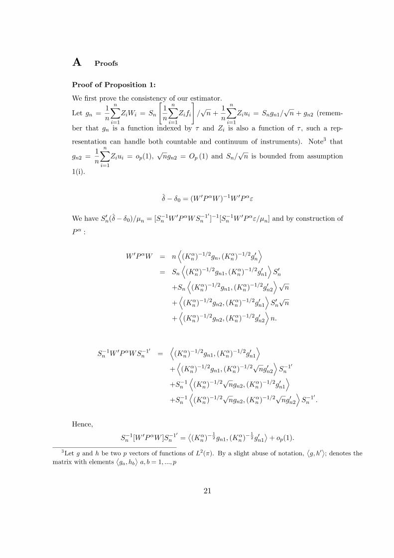
Proof of Proposition 1:

We �rst prove the consistency of our estimator.

Let gn =1

n

nXi=1

ZiWi = Sn

"1

n

nXi=1

Zifi

#=pn +

1

n

nXi=1

Ziui = Sngn1=pn + gn2 (remem-

ber that gn is a function indexed by � and Zi is also a function of � , such a rep-

resentation can handle both countable and continuum of instruments). Note3 that

gn2 =1

n

nXi=1

Ziui = op(1);pngn2 = Op (1) and Sn=

pn is bounded from assumption

1(i).

� � �0 = (W 0P�W )�1W 0P�"

We have S0n(�� �0)=�n = [S�1n W 0P�WS�10

n ]�1[S�1n W 0P�"=�n] and by construction of

P� :

W 0P�W = nD(K�

n )�1=2gn; (K

�n )�1=2g0n

E= Sn

D(K�

n )�1=2gn1; (K

�n )�1=2g0n1

ES0n

+Sn

D(K�

n )�1=2gn1; (K

�n )�1=2g0n2

Epn

+D(K�

n )�1=2gn2; (K

�n )�1=2g0n1

ES0npn

+D(K�

n )�1=2gn2; (K

�n )�1=2g0n2

En:

S�1n W 0P�WS�10

n =D(K�

n )�1=2gn1; (K

�n )�1=2g0n1

E+D(K�

n )�1=2gn1; (K

�n )�1=2png0n2

ES�1

0n

+S�1n

D(K�

n )�1=2pngn2; (K�

n )�1=2g0n1

E+S�1n

D(K�

n )�1=2pngn2; (K�

n )�1=2png0n2

ES�1

0n :

Hence,

S�1n [W 0P�W ]S�10

n =(K�

n )� 12 gn1; (K

�n )� 12 g0n1

�+ op(1):

3Let g and h be two p vectors of functions of L2(�). By a slight abuse of notation,g; h0

�; denotes the

matrix with elementsga; hb

�a; b = 1; :::; p

21

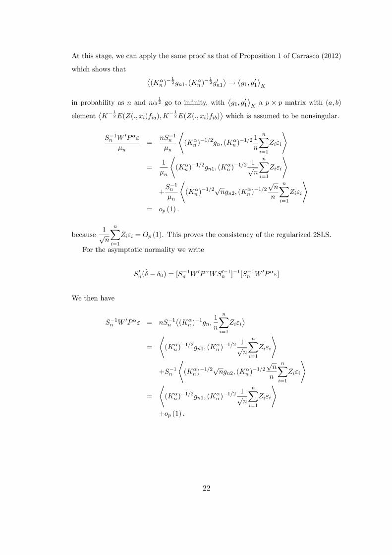
At this stage, we can apply the same proof as that of Proposition 1 of Carrasco (2012)

which shows that (K�

n )� 12 gn1; (K

�n )� 12 g0n1

�!g1; g

01

�K

in probability as n and n�12 go to in�nity, with

g1; g

01

�Ka p � p matrix with (a; b)

elementK� 1

2E(Z(:; xi)fia);K� 12E(Z(:; xi)fib)

�which is assumed to be nonsingular.

S�1n W 0P�"

�n=

nS�1n�n

*(K�

n )�1=2gn; (K

�n )�1=2 1

n

nXi=1

Zi"i

+

=1

�n

*(K�

n )�1=2gn1; (K

�n )�1=2 1p

n

nXi=1

Zi"i

+

+S�1n�n

*(K�

n )�1=2pngn2; (K�

n )�1=2

pn

n

nXi=1

Zi"i

+= op (1) :

because1pn

nXi=1

Zi"i = Op (1). This proves the consistency of the regularized 2SLS.

For the asymptotic normality we write

S0n(� � �0) = [S�1n W 0P�WS0�1n ]�1[S�1n W 0P�"]

We then have

S�1n W 0P�" = nS�1n(K�

n )�1gn;

1

n

nXi=1

Zi"i�

=

*(K�

n )�1=2gn1; (K

�n )�1=2 1p

n

nXi=1

Zi"i

+

+S�1n

*(K�

n )�1=2pngn2; (K�

n )�1=2

pn

n

nXi=1

Zi"i

+

=

*(K�

n )�1=2gn1; (K

�n )�1=2 1p

n

nXi=1

Zi"i

++op (1) :

22

Moreover, *(K�

n )�1=2gn1; (K

�n )�1=2 1p

n

nXi=1

Zi"i

+(2)

=(K�

n )�1gn1 �K�1g1;

1pn

nXi=1

Zi"i�

(3)

+K�1g1;

1pn

nXi=1

Zi"i)�:

The �rst term is negligible since(K�

n )�1gn1�K�1g1;

1pn

nXi=1

Zi"i)�� k(K�

n )�1gn1�K�1g1kk

1pn

nXi=1

Zi"ik = op(1)Op(1):

By the functional central limit theorem, we obtain the following resultK�1g1;

1pn

nXi=1

Zi"i�! N (0; �2"

g1; g

01

�K) as n and n�, �n go to in�nity.

We then apply the continuous mapping theorem and Slutzky lemma to show that

S0n(� � �0)d! N (0; �2"

g1; g

01

��1K):

By assumption, g1a = E(Z(:; xi)fia) belong to the range of K. Let L2(Z) be the

closure of the space spanned by fZ(x; �); � 2 Ig and g1 is an element of this space. If

fi 2 L2(Z) we can compute the inner product in the RKHS and show that

g1a; g1b

�K= E(fiafib):

This can be seen by applying Theorem 6.4 of Carrasco, Florens, and Renault (2007).

It follows that

S0n(� � �0)d! N

�0; �2"

�E�fif

0i

���1�This completes the proof of Proposition 1.

Proof of Proposition 2:

To prove this proposition we need some lemmas. The �rst lemma corresponds to lemma

A0 of Hansen, Hausman, and Newey (2008).

Lemma 1: Under assumption 1 if kS0n(�L��0)=�nk2=(1+k�Lk2)! 0 then kS0n(�L�

�0)=�nk ! 0.

proof: The proof of this lemma is the same as in Hansen, Hausman, and Newey

(2008).

23

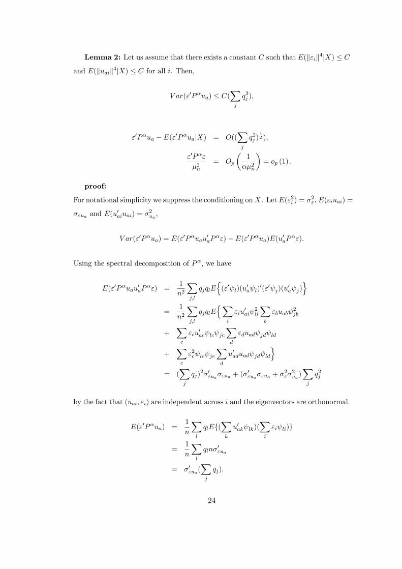
Lemma 2: Let us assume that there exists a constant C such that E(k"ik4jX) � C

and E(kuaik4jX) � C for all i. Then,

V ar("0P�ua) � C(Xj

q2j );

"0P�ua � E("0P�uajX) = O((Xj

q2j )12 );

"0P�"

�2n= Op

�1

��2n

�= op (1) :

proof:

For notational simplicity we suppress the conditioning onX. Let E("2i ) = �2", E("iuai) =

�"ua and E(u0aiuai) = �2ua ,

V ar("0P�ua) = E("0P�uau0aP

�")� E("0P�ua)E(u0aP�"):

Using the spectral decomposition of P�, we have

E("0P�uau0aP

�") =1

n2

Xj;l

qjqlEn("0 l)(u

0a l)

0("0 j)(u0a j)

o=

1

n2

Xj;l

qjqlEnX

i

"iu0ai

2li

Xb

"buab 2jb

+Xc

"cu0ac lc jc

Xd

"duad jd ld

+Xc

"2c lc jcXd

u0aduad jd ld

o= (

Xj

qj)2�0"ua�"ua + (�

0"ua�"ua + �

2"�2ua)Xj

q2j

by the fact that (uai; "i) are independent across i and the eigenvectors are orthonormal.

E("0P�ua) =1

n

Xl

qlEf(Xk

u0ak lk)(Xi

"i li)g

=1

n

Xl

qln�0"ua

= �0"ua(Xj

qj):

24

Thus

V ar("0P�ua) = (�0"ua�"ua + �

2"�2ua)Xj

q2j � C(Xj

q2j ):

The second conclusion follows by Markov inequality.

E�"0P�"

�= tr

�P�E

�""0��

= �2"(Xj

qj) = Op (1=�) :

Using the result for "0P�ua with " in place of ua, we obtain

V ar("0P�") � C(Xj

q2j ):

It follows that�"0P�"� E

�"0P�"

��=�2n = Op

0B@0@X

j

q2j

1A1=2 =�2n1CA = op

0@Xj

qj=�2n

1A :

Hence, the third equality holds.

Lemma 3: Let A =f 0P�f

nand B =

�W 0 �W

nwith �W = [y;W ] , there exist two

constants C and C 0 such that A � CIp and kBk � C 0:

Proof: By the de�nition of P�, we have (see Equation (1)):

A =f 0P�f

n=(K�

n )� 12 fn; (K

�n )� 12 f 0n�

with

fn =1

n

Xi

Zifi:

By Lemma 5(i) of Carrasco (2012) and the law of large numbers,

f 0P�f

n=f 0f

n+ op (1) = E(f 0ifi) + op(1)

as � goes to zero. Because E(f 0ifi) is positive de�nite, there exists a constant C such

that

A � CIp

25

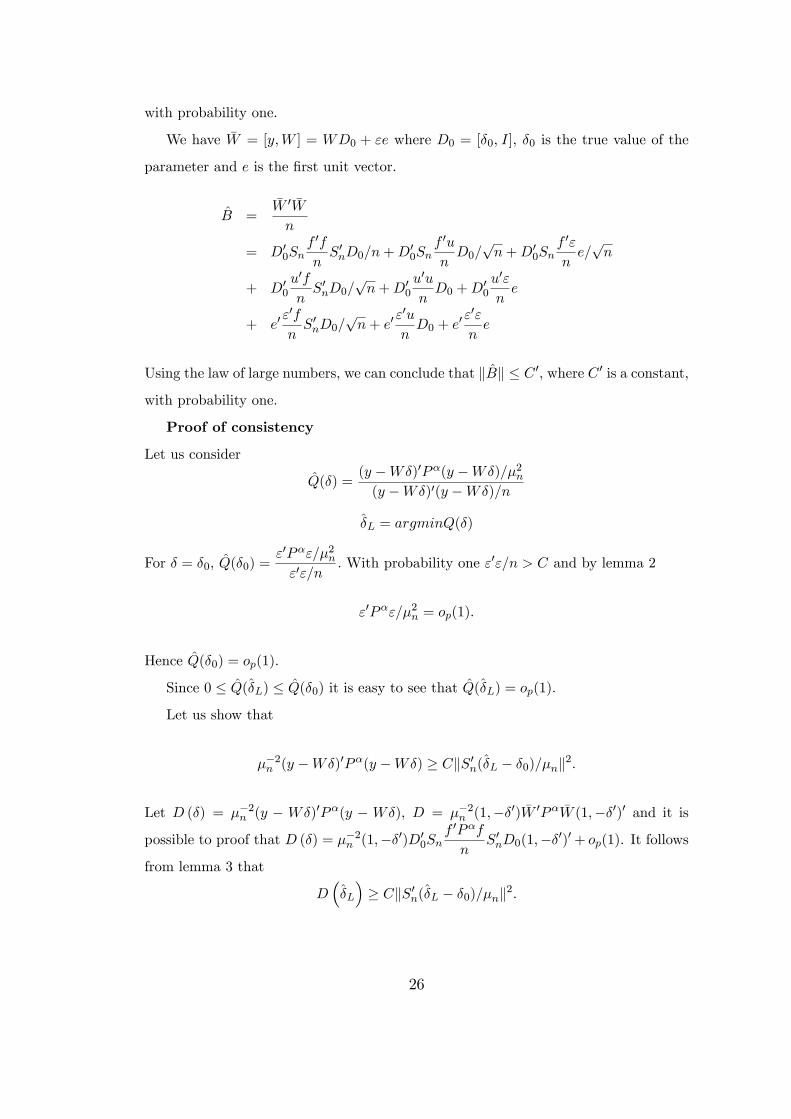
with probability one.

We have �W = [y;W ] = WD0 + "e where D0 = [�0; I], �0 is the true value of the

parameter and e is the �rst unit vector.

B =�W 0 �W

n

= D00Sn

f 0f

nS0nD0=n+D

00Sn

f 0u

nD0=

pn+D0

0Snf 0"

ne=pn

+ D00

u0f

nS0nD0=

pn+D0

0

u0u

nD0 +D

00

u0"

ne

+ e0"0f

nS0nD0=

pn+ e0

"0u

nD0 + e

0 "0"

ne

Using the law of large numbers, we can conclude that kBk � C 0, where C 0 is a constant,

with probability one.

Proof of consistency

Let us consider

Q(�) =(y �W�)0P�(y �W�)=�2n(y �W�)0(y �W�)=n

�L = argminQ(�)

For � = �0, Q(�0) ="0P�"=�2n"0"=n

: With probability one "0"=n > C and by lemma 2

"0P�"=�2n = op(1):

Hence Q(�0) = op(1).

Since 0 � Q(�L) � Q(�0) it is easy to see that Q(�L) = op(1).

Let us show that

��2n (y �W�)0P�(y �W�) � CkS0n(�L � �0)=�nk2:

Let D (�) = ��2n (y � W�)0P�(y � W�), D = ��2n (1;��0) �W 0P� �W (1;��0)0 and it is

possible to proof that D (�) = ��2n (1;��0)D00Sn

f 0P�f

nS0nD0(1;��0)0+ op(1). It follows

from lemma 3 that

D��L

�� CkS0n(�L � �0)=�nk2:

26

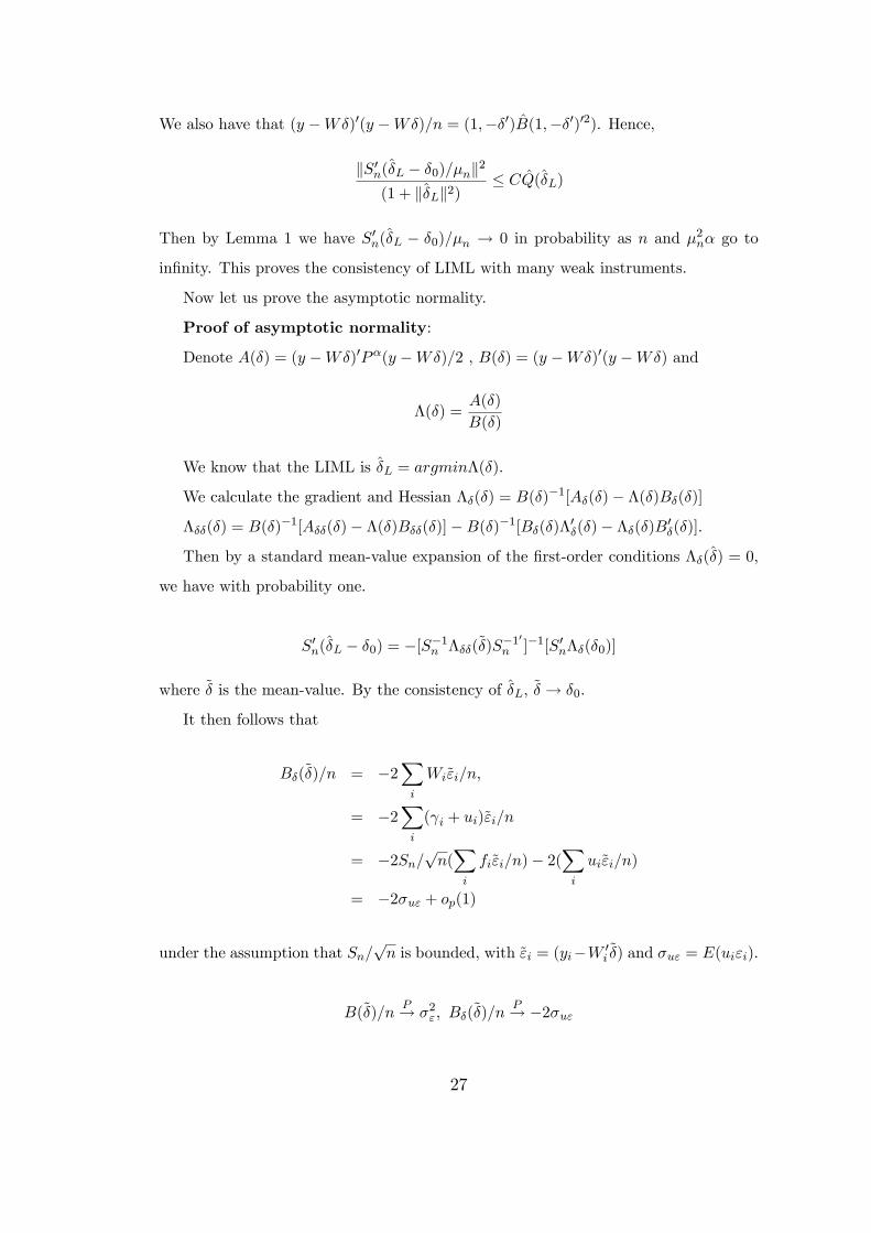
We also have that (y �W�)0(y �W�)=n = (1;��0)B(1;��0)02). Hence,

kS0n(�L � �0)=�nk2

(1 + k�Lk2)� CQ(�L)

Then by Lemma 1 we have S0n(�L � �0)=�n ! 0 in probability as n and �2n� go to

in�nity. This proves the consistency of LIML with many weak instruments.

Now let us prove the asymptotic normality.

Proof of asymptotic normality:

Denote A(�) = (y �W�)0P�(y �W�)=2 , B(�) = (y �W�)0(y �W�) and

�(�) =A(�)

B(�)

We know that the LIML is �L = argmin�(�):

We calculate the gradient and Hessian ��(�) = B(�)�1[A�(�)� �(�)B�(�)]

���(�) = B(�)�1[A��(�)� �(�)B��(�)]�B(�)�1[B�(�)�0�(�)� ��(�)B0�(�)]:

Then by a standard mean-value expansion of the �rst-order conditions ��(�) = 0;

we have with probability one.

S0n(�L � �0) = �[S�1n ���(~�)S�10n ]�1[S0n��(�0)]

where ~� is the mean-value. By the consistency of �L, ~� ! �0.

It then follows that

B�(~�)=n = �2Xi

Wi~"i=n;

= �2Xi

( i + ui)~"i=n

= �2Sn=pn(Xi

fi~"i=n)� 2(Xi

ui~"i=n)

= �2�u" + op(1)

under the assumption that Sn=pn is bounded, with ~"i = (yi�W 0

i~�) and �u" = E(ui"i).

B(~�)=nP! �2"; B�(

~�)=nP! �2�u"

27

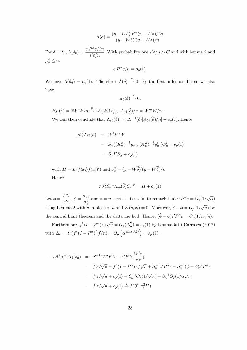
�(�) =(y �W�)0P�(y �W�)=2n

(y �W�)0(y �W�)=n

For � = �0, �(�0) ="0P�"=2n

"0"=n:With probability one "0"=n > C and with lemma 2 and

�2n � n;

"0P�"=n = op(1):

We have �(�0) = op(1). Therefore, �(~�)P! 0: By the �rst order condition, we also

have

��(~�)P! 0:

B��(~�) = 2W0W=n

P! 2E(WiW0i ); A��(

~�)=n =W 0�W=n:

We can then conclude that ���(~�) = nB�1(~�)[A��(~�)=n] + op(1): Hence

n~�2"���(~�) = W 0P�W

= Sn(K�

n )� 12 gn1; (K

�n )� 12 g0n1

�S0n + op(1)

= SnHS0n + op(1)

with H = E(f(xi)f(xi)0) and ~�2" = (y �We�)0(y �We�)=n:

Hence

n~�2"S�1n ���(~�)S

�10n = H + op(1)

Let � =W 0"

"0", � =

�u"�2"

and v = u� "�0. It is useful to remark that v0P�" = Op(1=p�)

using Lemma 2 with v in place of u and E (uivi) = 0. Moreover, ��� = Op(1=pn) by

the central limit theorem and the delta method. Hence, (�� �)"0P�" = Op(1=�pn).

Furthermore, f 0 (I � P�) "=pn = Op(�

2�) = op(1) by Lemma 5(ii) Carrasco (2012)

with �� = tr(f 0 (I � P�)2 f=n) = Op

��min(�;2)

�= op (1) :

�n~�2S�1n ��(�0) = S�1n (W 0P�"� "0P�"W0"

"0")

= f 0"=pn� f 0 (I � P�) "=

pn+ S�1n v0P�"� S�1n (�� �)"0P�"

= f 0"=pn+ op(1) + S

�1n Op(1=

p�) + S�1n Op(1=�

pn)

= f 0"=pn+ op(1)

d! N (0; �2"H)

28

as n, ��2n go to in�nity under the assumption �nS�1n ! S0.

The conclusion follows from the use of Slutzky theorem.

29