Efficient Join Synopsis Maintenance for DataWarehouse

Zhuoyue Zhao

University of Utah

zyzhao@cs.utah.edu

Feifei Li

University of Utah

lifeifei@cs.utah.edu

Yuxi Liu∗

University of Utah

louisja1@cs.utah.edu

ABSTRACTVarious sources such as daily business operations and sensors

from different IoT applications constantly generate a lot of

data. They are often loaded into a data warehouse system to

perform complex analysis over. It, however, can be extremely

costly if the query involves joins, especially many-to-many

joins over multiple large tables. A join synopsis, i.e., a small

uniform random sample over the join result, often suffices as

a representative alternative to the full join result for many

applications such as histogram construction, model training

and etc. Towards that end, we propose a novel algorithm

SJoin that can maintain a join synopsis over a pre-specified

general θ -join query in a dynamic database with continuous

inflows of updates. Central to SJoin is maintaining aweighted

join graph index, which assists to efficiently replace join

results in the synopsis upon update. We conduct extensive

experiments using TPC-DS and a simulated road sensor data

over several complex join queries and they demonstrate the

clear advantage of SJoin over the best available baseline.

CCS CONCEPTS• Information systems → Join algorithms; Data ware-houses; • Theory of computation→ Sketching and sam-pling.

KEYWORDSjoin synopsis; random sampling

ACM Reference Format:Zhuoyue Zhao, Feifei Li, and Yuxi Liu. 2020. Efficient Join Synop-

sis Maintenance for Data Warehouse. In Proceedings of the 2020∗The author was also affiliated with Shanghai Jiao Tong University. Work

was done during an internship at University of Utah.

Permission to make digital or hard copies of all or part of this work for

personal or classroom use is granted without fee provided that copies are not

made or distributed for profit or commercial advantage and that copies bear

this notice and the full citation on the first page. Copyrights for components

of this work owned by others than ACMmust be honored. Abstracting with

credit is permitted. To copy otherwise, or republish, to post on servers or to

redistribute to lists, requires prior specific permission and/or a fee. Request

permissions from permissions@acm.org.

SIGMOD’20, June 14–19, 2020, Portland, OR, USA© 2020 Association for Computing Machinery.

ACM ISBN 978-1-4503-6735-6/20/06. . . $15.00

https://doi.org/10.1145/3318464.3389717

ACM SIGMOD International Conference on Management of Data(SIGMOD’20), June 14–19, 2020, Portland, OR, USA. ACM, New York,

NY, USA, 16 pages. https://doi.org/10.1145/3318464.3389717

1 INTRODUCTIONA large volume of data is constantly generated from vari-

ous sources such as daily business operations, sensors from

different IoT applications, and etc. It is common to monitor

and perform complex analysis over these frequently updated

data. To explore the data, the data are often loaded into a

full-fledged data warehouse system where one can run vari-

ous complex analytical queries. Although the state-of-the-art

data warehouse systems that produce exact answers are op-

timized to achieve low response time, it can still be quite

slow, especially for a many-to-many join over multiple large

tables. Even worse, the queries may need to be frequently

re-run over the updated data to get the up-to-date results.

SELECT *FROM store_sales ss,store_returns sr,catalog_sales csWHERE ss.item_sk = sr.item_sk

AND ss.ticket_number = sr.ticket_numberAND sr.customer_sk = cs.customer_skAND ss.sold_date_sk <= cs.sold_date_sk

Figure 1: Q1: Linking store returns with subsequentcatalog purchases for correlation analysisTo give a concrete example (Figure 1), suppose we have

a business sales database with 3 tables. Both store_salesand store_returns have (item_sk,ticket_number) as theprimary key and customer_sk is not a key in any table.

An analyst may want to monitor and analyze a series of

events where a customer returns some store purchase and

subsequently places catalog orders, to study how they are

correlated for marketing purposes. To do that, the analyst

might issue query Q1 to identify the events and perform

analysis over the join result. Note that, store_returns ▷◁catalog_sales is many-to-many because the join attribute

customer_sk is not a key, which raises several issues:

• The join query can be prohibitively expensive to com-

pute regardless of the algorithm used, because the

result is simply too large. For instance in Q1, suppose

each customer places d catalog orders after a store re-

turn on average, the join size would be d times of the

size of store_returns, which can easily be orders of

magnitude larger than any of the base tables.

• It can be too expensive to perform analysis on the join

results because the input is too large. An example is

to build an equi-depth histogram on the number of

days elapsed before the second purchase happen after

the first one. Or the analyst may be tasked to build a

model to predict the subsequent catalog purchase after

the return based on the join result. All of these tasks

may take a very long time on the large join result.

• Incremental maintenance of the join result can also

be prohibitively expensive. To maintain an exact join

result, one has to at least compute the delta join result

associated with any base table update, which can be

quite large in a many-to-many join. After that, the

analysis on the join result needs to be incrementally

updated with the delta join result, or even worse, it

needs to be run again in full if incremental update is

unavailable for the analysis. Both of that contributes

to high latency in handling updates.

The crux of the problem is the high cost of exactly com-

puting a huge join. To avoid that, we can instead maintain

a join synopsis, i.e., a small uniform random sample of the

join results, for each pre-specified join query. It can serve as

a representative substitute to the full join results in many

tasks without the loss of too much accuracy. For example,

anf Nk -deviant approximation of an equi-depth k-histogram

over N items can be obtained from a random sample of size

O(k logNf 2 ) with high probability. Another important use case

is machine learning. There have been many studies showing,

both theoretically (e.g.,[27]) and in practice (e.g.,[12, 19]),

that it is feasible to use a small sample in lieu of the full data

to train a model with similar errors.

Our approach is also akin to incremental view mainte-

nance over pre-specified join queries but, instead of maintain-

ing all the join results which are too expensive to compute,

store and process, we maintain random samples of them. The

key challenge is to efficiently maintain it on the fly in face

of updates with minimal overhead. While there have been

works related to join synopsis maintenance for foreign-key

joins [1] in a dynamically updated database and random sam-

pling over join queries [5, 34] in a static database, it is, to our

best knowledge, still unclear how to maintain join synopses

for general join queries in a dynamically updated database.

Our contribution. To that end, we design a novel algo-

rithm SJoin (Synopsis Join) for maintaining join synopses

on general θ -join queries in a dynamically updated data-

base. In a nut shell, SJoin maintains a join synopsis for each

pre-specified query as well as several weighted join graph

indexes. The indexes encode weights, i.e., the number of join

results of a subjoin starting from a tuple, which allows us

to efficiently sample from the delta join results and the his-

torical join results to replace and/or replenish join results in

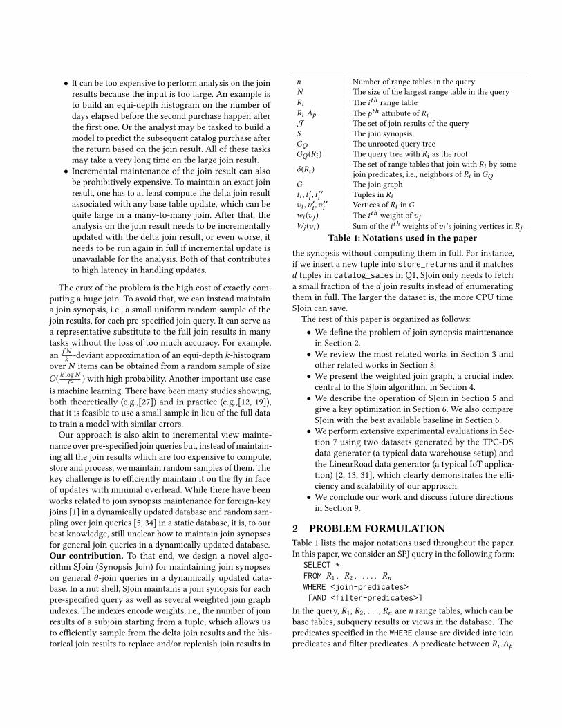
n Number of range tables in the query

N The size of the largest range table in the query

Ri The ith range table

Ri .Ap The pth attribute of RiJ The set of join results of the query

S The join synopsis

GQ The unrooted query tree

GQ (Ri ) The query tree with Ri as the root

δ (Ri )The set of range tables that join with Ri by some

join predicates, i.e., neighbors of Ri in GQG The join graph

ti , t′i , t′′i Tuples in Ri

vi ,v′i ,v′′i Vertices of Ri in G

wi (vj ) The ith weight of vjWj (vi ) Sum of the ith weights of vi ’s joining vertices in Rj

Table 1: Notations used in the paper

the synopsis without computing them in full. For instance,

if we insert a new tuple into store_returns and it matches

d tuples in catalog_sales in Q1, SJoin only needs to fetch

a small fraction of the d join results instead of enumerating

them in full. The larger the dataset is, the more CPU time

SJoin can save.

The rest of this paper is organized as follows:

• We define the problem of join synopsis maintenance

in Section 2.

• We review the most related works in Section 3 and

other related works in Section 8.

• We present the weighted join graph, a crucial index

central to the SJoin algorithm, in Section 4.

• We describe the operation of SJoin in Section 5 and

give a key optimization in Section 6. We also compare

SJoin with the best available baseline in Section 6.

• We perform extensive experimental evaluations in Sec-

tion 7 using two datasets generated by the TPC-DS

data generator (a typical data warehouse setup) and

the LinearRoad data generator (a typical IoT applica-

tion) [2, 13, 31], which clearly demonstrates the effi-

ciency and scalability of our approach.

• We conclude our work and discuss future directions

in Section 9.

2 PROBLEM FORMULATIONTable 1 lists the major notations used throughout the paper.

In this paper, we consider an SPJ query in the following form:

SELECT *FROM R1, R2, . . ., RnWHERE <join-predicates>[AND <filter-predicates>]

In the query, R1, R2, . . ., Rn are n range tables, which can be

base tables, subquery results or views in the database. The

predicates specified in the WHERE clause are divided into join

predicates and filter predicates. A predicate between Ri .Ap

and R j .Aq (whereAp andAq are two attributes) is considered

as a join predicate if it is in one of the following forms:

• Ri .Ap op cR j .Aq + d• |Ri .Ap − cR j .Aq | lt d ,

where op is one of <, <=, >, >=,=; lt is < or <=; and c,d are

constants. The definition is broad enough to include common

cases such as equi-join, band-join and so on, while it is also

confined to those that can be expressed as an open or close

range of one attribute in terms of the other, so that we can

utilize the common tree indexes to perform index joins.

Suppose J is the set of join results of query Q given the

data in the tables. A join synopsis S is a subset of J that

contains a uniform sample of the join results. There are three

different types of join synopses:

• Bernoulli join synopsis: each join result in J is inde-

pendently put into S with a fixed probability p.• Fixed-size join synopsis w/o replacement: a fixed num-

berm of distinct join results are selected into S from

J with equal probabilities.

• Fixed-size join synopsis w/ replacement: a fixed num-

ber ofm (potentially duplicate) join results are selected

into S from J with equal probabilities.

Problem formulation.Given a database and a user-specifiedn-table join query Q , we want to efficiently maintain a join

synopsis S of any of the three types upon any sequence of

insertions and deletions to any of the n tables. The join syn-

opsis should be ready to be returned at any time within an

O(1) response time, regardless of the sizes of the range tables

and how many insertions and deletions have happened.

3 BACKGROUNDJoin synopses are useful for saving query time by both avoid-

ing the full join computation and reducing the input size for

the subsequent operators in the query plan (e.g., aggrega-

tion, UDF). Contrary to samples produced by join sampling

algorithms that are designed for aggregations [11, 14, 15], it

is a uniform and independent sample of the join results and

can be used in many other applications with certain accu-

racy guarantees (e.g., using uniform samples for approximate

equi-depth histogram construction [4]) or without violating

assumptions (e.g., training set in machine learning which is

often assumed to be an i.i.d. sample of the population).

On the other hand, construction and maintenance of join

synopses is known to be a hard problem in the literature

because simply random sampling the range tables can only

yield very sparse results in a typical case. For example, taking

a p fraction of two tables to be joined only yields a p2 fractionof all the join results. The more table participates in a multi-

way join, the smaller fraction the final results will be. The

most related work is due to Acharya et al. [1] who studied

the maintenance of join synopses on a foreign-key join R1 ▷◁

𝑅Index

𝑅Index

𝑅

𝑅

Build

Build

𝑅 ⋈ 𝑅

Bernoulli/ Reservoir Sampling Join

Synopsis

SJ Operator

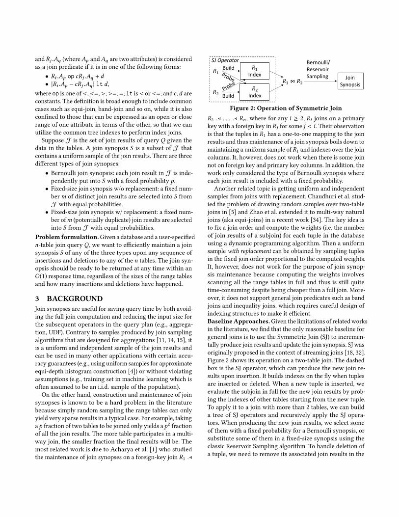
Figure 2: Operation of Symmetric JoinR2 ▷◁ . . . ▷◁ Rn , where for any i ≥ 2, Ri joins on a primary

key with a foreign key in R j for some j < i . Their observationis that the tuples in R1 has a one-to-one mapping to the join

results and thus maintenance of a join synopsis boils down to

maintaining a uniform sample of R1 and indexes over the join

columns. It, however, does not work when there is some join

not on foreign key and primary key columns. In addition, the

work only considered the type of Bernoulli synopsis where

each join result is included with a fixed probability.

Another related topic is getting uniform and independent

samples from joins with replacement. Chaudhuri et al. stud-

ied the problem of drawing random samples over two-table

joins in [5] and Zhao et al. extended it to multi-way natural

joins (aka equi-joins) in a recent work [34]. The key idea is

to fix a join order and compute the weights (i.e. the number

of join results of a subjoin) for each tuple in the database

using a dynamic programming algorithm. Then a uniform

sample with replacement can be obtained by sampling tuples

in the fixed join order proportional to the computed weights.

It, however, does not work for the purpose of join synop-

sis maintenance because computing the weights involves

scanning all the range tables in full and thus is still quite

time-consuming despite being cheaper than a full join. More-

over, it does not support general join predicates such as band

joins and inequality joins, which requires careful design of

indexing structures to make it efficient.

BaselineApproaches.Given the limitations of relatedworks

in the literature, we find that the only reasonable baseline for

general joins is to use the Symmetric Join (SJ) to incremen-

tally produce join results and update the join synopsis. SJ was

originally proposed in the context of streaming joins [18, 32].

Figure 2 shows its operation on a two-table join. The dashed

box is the SJ operator, which can produce the new join re-

sults upon insertion. It builds indexes on the fly when tuples

are inserted or deleted. When a new tuple is inserted, we

evaluate the subjoin in full for the new join results by prob-

ing the indexes of other tables starting from the new tuple.

To apply it to a join with more than 2 tables, we can build

a tree of SJ operators and recursively apply the SJ opera-

tors. When producing the new join results, we select some

of them with a fixed probability for a Bernoulli synopsis, or

substitute some of them in a fixed-size synopsis using the

classic Reservoir Sampling algorithm. To handle deletion of

a tuple, we need to remove its associated join results in the

interface View {UINT8 length();TID[] get(UINT8 index);

}Figure 3: Iterator interface of the non-materializeddelta join viewsynopsis. In the case of a fixed-size synopsis, we further need

to re-compute the full join to replace the missing samples.

Thus , in all cases, the complexity of insertion or deletion is

at least linear to the subjoin or the full join size regardless

of how the join and the indexes are optimized. That makes

updates very expensive, especially for many-to-many joins.

4 WEIGHTED JOIN GRAPH INDEXBefore we present the SJoin algorithm, we introduce the

weighted join graph, an index central to the operation of the

SJoin algorithm. The index is crucial for efficient synopsis

maintenance because it serves two purposes:

• it can create a temporary non-materialized delta joinview over the subjoin results associated with the new

tuple upon insertion of a tuple into any range table.

The view provides an array-like random access inter-

face (Figure 3). Over that we can apply a variant of

reservoir sampling for all three types of synopsis.

• it can be used to re-draw uniform and independent

samples from the entire join results to replenish a fixed-

size synopsis, when some join samples have to be re-

moved from the synopsis because their comprising

tuples are deleted from the range tables.

In a nut shell, a weighted join graph encodes all theweights

needed to extract uniform sampling over a subjoin starting

with an arbitrary tuple in any table. In this section, we will

show how the weighted join graph is constructed and effi-

ciently maintained, and how to perform these two tasks.

Throughout this section and the section after, we will use a

5-table acyclic join query as a running example (Figure 4). In

the query,R2,R4 andR5 all join withR3 on different attributes

while R1 joins with R2, and there are no filter predicates.

4.1 Unrooted query treeIn a conventional database, the query plan for join is often

organized as a rooted tree, which implicitly defines a join

order. In contrast, we build an unrooted query tree given a

pre-specified join query in SJoin. It is unrooted for a reason:

we might consider subjoins starting from any tables as new

tuples can be inserted into any range tables. The query tree

is constructed as follows. Each range table in the query is

represented as a vertex in the query tree and there is an edge

between two vertices if there is a join predicate between

the two corresponding range tables. If the resulting graph

is acyclic, which can be easily determined by a simple tra-

versal of the graph, we already have an unrooted query tree,

SELECT *

FROM R1, R2, R3, R4, R5WHERE R1.A = R2.A

AND R2.B = R3.B

AND R3.C = R4.C

AND R3.D = R5.DFigure 4: A 5-way equi-join query example

𝑅 𝑅 𝑅𝐶 𝐷

𝑅

𝑅

𝐵

𝐴

Figure 5: Query Tree GQfor the running example

denoted as GQ . The query is called an acyclic query in this

case. If a cycle is found during the traversal, we arbitrarily

remove an edge on the cycle and treat the corresponding join

predicate as a filter predicate. Thus we will eventually end

up with an unrooted query treeGQ for cyclic queries as well.

For instance, Figure 5 shows the resulting query treeGQ for

the running example. Since the query is already acyclic, we

do not have to remove any edges to make it acyclic.

4.2 Weighted join graphA join graphG is built on a database instance. Figure 6 shows

the join graph of the running example for the instance shown

at its top. For simplicity, only the join attributes are shown

and each row has a unique row ID. The vertices are the

distinct join attributes projected from the tuples in the tables.

An edge between two vertices means that the corresponding

tuples satisfy the join conditions. For example, the vertex

with join attributes (2,1,2) in R3 corresponds to tuples 1, 3in R3. Its neighbors in R2,R4,R5 are those that satisfy the

corresponding join predicates. In the remainder of this paper,

vertices (resp. tuples) in R j are denoted asvj ,v′j ,v′′j , . . . (resp.

tj , t′j , t′′j , . . .), where we use the subscript to imply the range

table they belong to and the prime signs to differentiate

between different vertices (resp. tuples) from the same table.

For an n-table query on a given database instance, each

join result can be mapped to exactly one subgraph of G that

is homomorphic to GQ and covers exactly one vertex in

each range table. On the other hand, one such subgraph may

correspond to multiple join results because of tuples with

duplicate join attribute values. The vector w represents a

vector of weights which will be defined shortly. We denote

a join result as a 5-tuple of the row IDs of its comprising

tuples in the range tables. Hence, join result (3, 1, 3, 0, 2)corresponds to the subgraph highlighted in orange outlines.

In the mean time, there are 23 other join results that the

outlined subgraph corresponds to.

LetGQ (Ri ) be a rooted query tree by setting Ri as the rootofGQ . It actually corresponds to a query plan ofQ that starts

from a tuple in Ri , denoted as Qi . Each subtree at root R jin GQ (Ri ) corresponds to a subjoin of Q , denoted as Qi (R j ).Hence, for each table R j , there are up to n possible different

subjoins that starts with R j . With that, we define the set of

weights of vertices as in Definition 4.1.

Row ID A

0 1

1 2

2 2

3 1

𝑅Row ID A B

0 1 1

1 1 2

2 2 2

𝑅

Row ID B C D

0 1 1 1

1 2 1 2

2 2 2 2

3 2 1 2

𝑅Row ID C

0 1

1 2

2 1

3 2

𝑅Row ID D

0 1

1 2

2 2

3 2

𝑅

1 2

1,1 1,2 2,2

1,1,1 2,1,2 2,2,2

1 2 1 2𝑅 𝑅

𝑅

𝑅

𝑅 ID = [0,3] ID = [1,2]𝑤 = [40,2,2,2,2] 𝑤 = [36,2,2,2,2]

ID = [1,3]𝑤 = [2,2,2,24,2]

ID = [2]𝑤 = [18,36,2,2,2]

ID = [1]𝑤 = [18,36,2,2,2]

ID = [0]𝑤 = [2,4,2,2,2]

ID = [2]𝑤 = [6,6,24,12,8]

ID = [1,3]𝑤 = [12,12,48,24,16]

ID = [0]𝑤 = [2,2,4,2,4]

ID = [0,2]𝑤 = [2,2,2,52,2]

ID = [0]𝑤 = [1,1,1,1,4]

ID = [1,2,3]𝑤 = [3,3,3,3,72]

Figure 6: Join Graph of the running example on the database instance shown atthe top. Non-join attributes in the tables are omitted in the figure. Each vertex hasa row ID list ID and its 5 weights. The weights in red are always the same as oneof the the others. The subgraph in orange corresponds to 24 join results.

𝑅𝑅 𝑅

Subgraph 2

Subgraph 1

Subgraph 3

𝑅

…

𝑅

Figure 7: A stream R j onlyhas d+1 unique weight func-tions if its degree is d in GQ .

Definition 4.1. LetAj be the set of join attributes in R j andvj be a vertex in R j . For a subtree in GQ that corresponds to

subjoin Qi (R j ), let Ri (R j ) be the set of tables in the subtree.

Then ith weight of vj is defined as

wi (vj ) = | ▷◁ (Ri (R j ) − {R j }) ▷◁ {tj ∈ R j |πAj tj = vj }|,

i.e., the number of results of all tuples that have the same

join attribute values as vj in R j joining the other tables in

Qi (R j ). For instance, let v3 be the vertex (2,1,2) and t3, t′3be

tuples 1,3 in R3. Thenw1(v3) = |{t3, t′3} ▷◁ R4 ▷◁ R5 | = 12.

The weights of each vertex in the running example are

shown as a vector with a length of 5 to the right of it. Note

that, for a vertex vj , there might be weights that are always

the same. For example,w1(v3) is always the same asw2(v3)for any v3 ∈ R3. This happens when they correspond to

the number of join results of the same subjoin and we want

to avoid computing and storing them for more than once.

Fortunately, it can be easily determined with Theorem 4.2.

Theorem 4.2. wi (vj ) ≡ wi′(vj ) iff Ri′ is not in the subtreeof GQ (Ri ) with the subtree root being R j .

For example, we can determine thatw1(v3) ≡ w2(v3) fromthe fact that the subtree rooted at R3 inGQ (R1) only includes

tables R3,R4,R5, not R2. In contrast,w1(v3) . w3(v3) becauseR3 is in that subtree.

Corollary 4.3. There are only d + 1 unique weight func-tions for the vertices in a table R j if its degree in GQ is d .Corollary 4.4. There are 3n − 2 unique weight functions

across all vertices.A further observation is Corollary 4.3. This can be ex-

plained with the general example shown in Figure 7, where

R j has d = 3 neighbors in GQ . The entire query tree can be

partitioned into 4 connected components, including three

that contain the neighbors Ri1 ,Ri2 ,Ri3 respectively, and R j it-self. Take subgraph 1 as an example. Any Ri′

1

in the subgraph

is not in the subtree ofGQ (Ri1 ) rooted at R j . By Theorem 4.2,

wi1 (vj ) ≡ wi′1

(vj ). Similar arguments also apply to subgraphs

2 and 3. The last unique weight isw j (vj ), which is the size

of the entire join and thus is different from any other ones.

Corollary 4.4 follows since the total degree of GQ is 2n − 2.

4.3 Index implementationInstead of using an explicit graph representation like adja-

cency list, we build multiple indexes over the vertices to

implicitly represent the join graph and encode the weights.

For each table Ri , we build a hash index Hi over the vertices

to facilitate fast look ups with join attribute values. It will be

looked up when we need to map a tuple to its corresponding

vertex during insertion or deletion. We further build one

aggregate tree index (which are AVL trees in our in-memory

implementation) over each join attributeA of vertices in each

table Ri , denoted as Ii (A) and there are 2n−2 of them. The dif-

ference between an aggregate tree index and an ordinary tree

index is the former can maintain subtree aggregates of some

numeric values in the vertices, which can be used to find the

smallest vertex (w.r.t. the join attribute the tree is built on)

whose prefix sum of the numeric value is greater than some

threshold (similar to std::lower_bound() in C++) and com-

pute subtree sums in any interval. In our case, we store all

the unique weights in each vertex and maintain subtree ag-

gregates of them. Let the set of Ri ’s neighbors inGQ be δ (Ri ).For a vertex vi in Ri , w j (vi ) and its subtree aggregates are

maintained in the Ii (A) if R j ∈ δ (Ri ) and their join predicate

is on column Ri .A. A special case iswi (vi ), which along with

its subtree aggregates are maintained in an arbitrarily chosen

tree index of Ri , denoted as Ii (A0). In addition, we also cache

the total weights of the joining vertices in R j with respect to

GQ (Ri ):Wj (vi ) =∑vj ∈Rj :vj ▷◁vi wi (vj ), as they may often be

used in computation of weights but seldom updated.

1 2

2

Aggregate AVL Index 𝐼 𝐵

Hash Index 𝐻

2,1,21,1,1 2,2,2𝑅

ID List

Tree pointers

Subtree sum

Cached neighbor sum weights

Unique Weights

1 2

1

Aggregate AVL Index 𝐼 𝐶

1 2

2

Aggregate AVL Index 𝐼 𝐷

Figure 8: Indexes over R3 in the running exampleFor example, we build 3 aggregate tree indexes over columns

B,C , D of R3 respectively, as shown in Figure 8. We maintain

subtree aggregates ofw2(v3),w3(v3) in I3(B);w4(v3) in I3(C);and w5(v3) in I3(D). One vertex is a single data structure

shared by all the relevant indexes with tree pointers embed-

ded into it. All fields in the vertex (tree pointers, weights and

etc.) are accessed with an offset from the beginning from the

structure, with the exception of the variable length ID list,

which is implemented as a structure header with two point-

ers to the beginning and the end of the list. All the offsets can

be determined by the query planner based on the unrooted

query tree in initialization so there will be no overhead in the

runtime. The benefit of this design is that we do not need to

search the entire AVL index for the corresponding tree nodes

when we find a vertex through the hash index or another

AVL index, which is very common in the maintenance and

operation of the weighted join graph index.

4.4 Index maintenanceWe explain how the weighted join graph index is updated on

each tuple insertion in this subsection. Deletion can be han-

dled by reversing the operations in the insertion algorithm

and thus is omitted for brevity.

Denote the set of Ri ’s neighbors in GQ as δ (Ri ) and the

join attribute of Ri in the join predicate between Ri and R j asAi, j . Algorithm 1 shows the process of inserting a new tuple

ti to the weighted join graph index. On line 13, the algorithm

first tries to find an existing vertexvi that corresponds to thetuple or create one if it does not exist using the hash index

Hi . In the case it is newly created, we populate the cache

of the total weights of joining vertices in neighbor tables

Wj (vi ). On line 16 and 19, we compute all the weights for viusing the cached total weights with Equation 1:

w j (vi ) = vi .ID.length() ×∏

Rj :Rj ∈δ (Ri )∧Rj,Ri

Wj (vi ). (1)

The equation holds for i = j because the weight is the totalnumber of join results ofvi which is the size of the Cartesian

product among the tuple ID list and the subjoin results for

each child. Similarly, it holds for i , j because in that case,

the weight is the size of the Cartesian product among the

tuple ID list and the subjoin results for each child except

Algorithm 1: Insert a new tuple to the weighted join

graph index

Input: An inserted tuple ti in Ri1 def updateNeighbor(i, j,u)

//Ri: parent table

//Rj: child table to be updated

//u: ordered list of key-∆w pairs

2 u ′ ← an array of empty ordered maps ;

3 foreach ( (key,∆w) ∈ u )4 foreach ( vj that join with the key )5 Wi (vj )+ = ∆w ;

6 recomputew j (vj ) ;

7 foreach ( Rj′ ∈ δ (Rj ) − {Ri } )8 w ′ ← w j′(vj ) ;

9 recomputew j′(vj ) ;

10 u ′[j ′][vj .Aj, j′]+ = w j′(vj ) −w′;

11 foreach ( Rj′ ∈ δ (Rj ) − {Ri } )12 updateNeighbor(j, j ′,u ′[j ′])

13 vi ← find or insert the corresponding vertex in Hi ;

14 if vi is a new vertex then15 Wj (vi ) ←

∑vj ∈Rj :vj ▷◁vi wi (vj ) for all Rj ∈ δ (Ri ) ;

16 computewi (vi );

17 foreach ( Rj ∈ δ (Ri ) )18 w ′ ← w j (vi ) ; //0 if it’s a new vertex

19 computew j (vi );

20 updateNeighbor(i, j, {(vi .Ai, j ,w j (vi ) −w′)})

R j . Whenever a weightw j (vi ) is updated, vi is inserted into

Ii (Ai, j ) (Ii (A0) in case i = j) if not already existent in the

tree index, and subtree aggregates are re-computed up to the

index root. Finally, the process recurses on reachable vertices

in the join graph with the updateNeighbor function on lines1-12. To do that, we create an ordered mapu where the key is

the join attribute value of the parent and the value is the total

delta weight of that join attribute for each table. In the update

of R j from a parent table Ri , all weights of vj exceptwi (vj )for all verticesvj that join some keys inu need to be updated.

Note that the nested for loops lines 3-4 are essentially a join

between the sorted list u and the set of vertices in Ri . Forequi-join, an index nested loop suffice. It, however, can incur

O(N 2) cost in the worst case for band/range joins. Thus,

in the latter case, we perform the join on lines 3-4 using

the merge process in the sort-merge join. Because the delta

weight can be accumulated on the fly, we only need to update

one vertex once, which means a linear time complexity for

each execution of the updateNeighbor function.

Theorem 4.5. Let h(vi ) be the number of vertices reach-able from the corresponding vertex vi of a tuple ti in theweighted join graph. It takes O(h(vi ) logN ) time to maintainthe weighted join graph upon inserting/deleting ti , where N isthe size of the largest range table given the database instance.

Algorithm 2:Mapping a join number to a join result

Input: A join number l , the query tree root RiOutput: The corresponding join result t = (t1, t2, . . . , tn )

1 def mapJoinNumber(j,vj , l)//Rj: table being partitioned

//vj: mapped vertex from Rj//l: remaining join number

2 w ′ ← wi (vj )/vj .ID.lenдth() ;

3 t[j] = vj .ID[⌊l/w′⌋] ;

4 l ← l modw ′ ;

5 foreach ( Rj ’s child Rk in GQ (Ri ) )6 W ←

∑vk :vk ▷◁vj wi (vk ) ;

7 l ′ ← l modW ;

8 l ← ⌊l/W ⌋ ;

9 vk ← min{vk |∑v ′k :v

′k ▷◁vj∧v

′k<vk

wi (v′k )} ;

10 mapJoinNumber (k , vk ,

l ′ −∑v ′k :v

′k ▷◁vj∧v

′k<vk

wi (v′k ));

11 vi ← min{vi |l <∑v ′i<vi

wi (v′i )} ;

12 mapJoinNumber(i,vi , l −∑v ′i<vi

wi (v′i ))

With that, inserting/deleting a tuple in the weighted join

graph index only incurs a linear cost in terms of the number

of reachable vertices from vi in the join graph, a cost that

is always smaller than that of the index nested loop in SJ

starting from the inserted/deleted tuple. To show that, we

count how many index accesses there are. Consider each

vertex vj reachable from vi , which corresponds to multiple

tuples in R j and each of which will be accessed via index in

SJ. In other words, SJ performs an additional index access

for every partial join result starting from ti , which can be

orders of magnitudes larger than h(vi ). For instance, supposewe are doing the following join query R1 ▷◁ |R1 .A−R2 .A | ≤dR2 ▷◁ |R2 .A−R3 .A | ≤d R3, and there are k tuples on average with

the same value of A in both R2 and R3. Starting from a tuple

t1, SJ performs 1+ (2d + 1)k + ((2d + 1)k)2 index accesses, i.e.,a O(d2k2 logN ) cost. In contrast, the cost of weighted join

graph maintenance in SJoin is only O(d logN ).

4.5 Random access to join resultsThe main operation that the weighted join graph index pro-

vides is random access to the join results via join numbers.

Let J = |J |, i.e., the total number of join results in the data-

base instance. A join number is an integer in [0, J − 1] thatis mapped to exactly one join result, which works just like

an array index in a typical programming languages. In a

nut shell, we define the mapping from a join number to a

join result by recursively partitioning the domain of the join

numbers proportional to the weights in the join graph, in

the order of preorder traversal ofGQ (Ri ) for some Ri . Hence,there can be n different mappings from the join numbers to

the join results for an n-table join, each with respective to a

different query tree root Ri .

For the mapping with respect to GQ (Ri ), we totally order

all vertices in a table R j other than Ri , in the increasing order

of its join attribute value in its join predicate to its parent

and arbitrarily break tie when there are equal values. The

vertices of the tree root Ri are instead totally ordered by

the first join attribute value (which is actually an arbitrary

choice) and ties are broken arbitrarily. For example, R2 in the

running example is ordered by the attribute value of column

Awith respect toGQ (R1), while R1 is ordered by the attribute

value of its first column that happens to be A as well.

The mapping with respect to GQ (Ri ) is shown as a func-

tion in Algorithm 2, whichmaps a join number l ∈ [0, J−1] tothe corresponding join result. We will explain the recursive

process using the running example of l = 30 with respective

toGQ (R1). The algorithm recursively calls mapJoinNumber()to partition the domain of the join numbers, identifies the

subdomain that the join number is in and remaps the subdo-

main to start from 0. On each table, it involves 3 steps:

(1) (Intra-table partition) In this step, the domain of

the join number is partitioned into consecutive sub-

domains that are proportional to wi (vk ), in the total

order of vk ’s that join the previous selection of vertex

vj (all vertices in the case of root). Then we find a vkthat corresponds to the subdomain that the remaining

join number l is in and recursively call the function

on vk with an adjusted remaining join number. In the

running example, the domain is initially [0, 75]. It’sdivided into two subdomains [0, 39] and [40, 75] corre-sponding to vertex (1) and (2) in R1 (lines 11-12). Since

l = 30 falls into [0, 39], mapJoinNumber is called on

vertex (1) with l ′ = 30. Note that the lower bound of

the subdomain, which happens to be 0, is subtracted

from l to obtain the new remaining join number l ′.(2) (Intra-vertex partition) In the second step, the do-

main of the join number is further partitioned into

subdomains of equal lengths for tuples listed in the ID

list. Continuing with the running example after the

first step, we have two subdomains [0, 19] and [20, 39]for tuple 0 and 3 in R1 respectively (lines 2). Since

30 ∈ [20, 39], tuple 3 is selected as part of the join re-

sult (line 3), and the domain of l is readjusted to [0, 19]by modulo that by the length w ′ of the subdomains,

yielding the remaining join number of l = 10.

(3) (Inter-table partition) The final step projects the do-main of the join number into several subdomains, each

with a length of the total weight of joining vertices in

one of the child table ofR j inGQ (Ri ). Suppose the childtables are Rk1 ,Rk2 , . . . ,Rknj from left to right, and the

total weights of joining vertices in each of them are

W1,W2, . . .Wnj respectively. Then the remaining join

Join Synopsis Spec:CREATE SYNOPSIS S ON (

SELECT *FROM 𝑅 , R , R , R , RWHERE …)

FIXED SIZE 4 WO REPLACEMENT;

ID List

Tree pointers

Subtree sum

Cached neighbor sum weights

Unique Weights

Struct 𝑣

ID List

Tree pointers

Subtree sum

Cached neighbor sum weights

Unique Weights

Struct 𝑣

ID List

Tree pointers

Subtree sum

Cached neighbor sum weights

Unique Weights

Struct 𝑣

ID List

Tree pointers

Subtree sum

Cached neighbor sum weights

Unique Weights

Struct 𝑣

ID List

Tree pointers

Subtree sum

Cached neighbor sum weights

Unique Weights

Struct 𝑣

Join graph vertex structs

① Query Planning

𝑅

𝑅

𝑅

𝑅

𝑅

Unrooted query tree

A

B

C D

1 2

1,1 1,2 2,2

1,1,1 2,1,2 2,2,2

1 2 1 2

Weighted Join Graph Index

𝑅 𝑅 𝑅 𝑅 𝑅

Range Tables

(0,0,0,2,0) (3,1,3,0,2) (2,2,2,1,1) (2,2,2,3,3)

Join SynopsisPersistent states:J=76 m=4n=4 s=5

② a. Index Creation

③ Insert/Delete 𝑡Online DML statements

④ Index Maintenance

⑤a. Replace samples via delta view for insertion

⑤b. Re-draw samples for deletion

⑥Return synopsis upon user request

Figure 9: Operation of the SJoin algorithmnumber is decomposed as nj join numbers in the sub-

domains, denoted as l1, l2, . . . lnj , with the following

mapping: l =∑nj

i=1 lj∏i−1

i′=1Wi′ . Then the process con-

tinues on each join number in the subdomains from

step 1 intra-table partition. In the running example,

the join number does not change after step 3 applies to

vertex (1) in R1 because it only has one child R2. Fast

forward to the moment when we are at vertex (2,1,2)

in R3 with the remaining join number l = 2. Then

we map it to two join numbers 0 and 1 for R4 and R5

respectively (lines 6-8).

It can be shown that the time complexity of Algorithm 2 is

O(n logN ) because line 6 takes O(1) time by simply reading

the cached valueWk (vj ); line 9, 11 and the remaining join

number computation on line 10, 12 can be implemented with

the aggregate tree indexes in O(logN ) time.

Recall the two tasks listed at the beginning of this sec-

tion. They can be implemented with Algorithm 2. For the

non-materialized delta join view, we find that the join num-

bers of all the new join results involving ti are in a consec-

utive subdomain with respect to GQ (Ri ), upon insertion a

new tuple ti in table Ri . Let vi be the corresponding vertexof ti , U =

∑v ′i<=vi

wi (v′i ) and w ′ = wi (vi )/vj .ID.lenдth().

Then the subdomain is [U −w ′,U − 1]. For the view V of ti ,V .length() = w ′ andV .get(index) can simply invoke Algo-

rithm 2 with l = U −w ′+ index and Ri . Re-drawing uniformsample from all join results boils down to drawing a random

join number in l = [0, J − 1] and invoking Algorithm 2 with

l and R1 (the choice of the query tree root can be arbitrary).

5 SJOIN ALGORITHMIn this section, we give an overview of the design of the SJoin

algorithm, and then provide details of how the join synopsis

is maintained with insertion and deletion of tuples in SJoin.

5.1 Algorithm overviewFigure 9 shows the operation of the SJoin algorithm. At data-

base creation, the query planner will build the unrooted

query tree for the join and automatically compute the offsets

of the vertex data structures in the weighted join graph index

based on the pre-specified query. It then creates an empty

weighted join graph. Given the pre-specified synopsis type

and parameters, the query planner initializes the join synop-

sis and some persistent states for synopsis maintenance.

The range tables are stored as ordinary heap files in the

database. The only special requirement is that the system

can associate a unique tuple identifier (or TID) to each tuple

across insertion and deletion. In some systems, such identi-

fiers are already available. If TID is not available, we attach an

additional monotonically increasing row ID column to each

table, like what we’ve shown in the running example in Fig-

ure 6. A tuple can be identified by the pair of its (range) table

ID and its row ID, denoted as t(table ID, index). For example,

t(3,2) denote the tuple with index 2 in R3. In the remainder

of this paper, we assume the latter is the representation of

a TID. Note that the same table may appear multiple times

as different range tables in the FROM clause. They can be

stored in the same heap file but they must be identified as

different range tables in the join. This arrangement allows

us to represent a join result uniquely as a tuple of the row

IDs of the comprising tuples in the range tables. For instance,

join result (1,2,0,3,2) is comprised of tuples t(1,1), t(2,2),t(3,0), t(4,3) and t(5,2).

The weighted join graph is updated whenever a range

table is updated. As described in Section 4, the weighted

join graph can provide two functionalities: providing a non-

materialized delta join view with random access upon inser-

tion of a tuple and re-drawing samples from all join results.

The join synopsis is updatedwhenever there are new/deleted

join results associated with an insertion/deletion. For in-

serted tuples, the synopsis is updated by applying a variant of

reservoir sampling to the delta join view. For deleted tuples,

the persistent state of the reservoir sampling is adjusted to

reflect a reduced size of join results in the database instance.

A fixed-size synopsis is further replenished with re-drawn

samples if its size falls below the specified size. The join

synopsis is always ready to be returned at any time, upon

a user request. Here, we assume the system fully serialize

all updates and synopsis requests, which can be done using

simple concurrency control schemes such as locking.

Filter Handling. There could be additional filter predicatesunaccounted for the join tree. The most common ones are

single-table filters such as A op c for some constant. They

can be applied as a pre-filter prior to insertion of tuples

into the range tables. The range tables are then replaced

by an indirection table where each row stores an TID to

a tuple in the range table that satisfies the filter. A lesser

common scenario are multi-table filters, which could be due

to cyclic join queries or user-defined predicates. These are

applied on top of the join synopsis upon user request. It may,

however, reduce the number of valid samples in the synopsis

and make it lower than specified in fixed-size sampling. To

ensure the resulting synopsis size is larger than desired with

high probability, we can estimate the selectivity of the multi-

table filter predicates f using existing system statistics and

enlarge the synopsis size by a factor of O(1/f ) on the fly.

5.2 Tuple insertion

Algorithm3: Join synopsis maintenance with a view

Input: Synopsis sizem or sampling rate p, Join result view

V1 Persistent state:2 S ← initialize-reservoir() ; //join synopsis

3 n ← 0 ; //# of valid join result samples

4 J ← 0 ; //# of join results skipped and/or

selected

5 s ← 0 ; //remaining skip number

6 Pseudocode:7 i ← 0 ;

8 while i < V .length() do9 if i + s >= V .length() then10 J ← J +V .length() − i ;

11 s ← s − (V .length() − i) ;

12 break;13 i ← i + s ;

14 J ← J + 1 ;

15 t ← V .get(i);

16 Update S with t ;

17 s ← drawSkipNumber(m, n, J) ;

An insertion of a tuple involves inserting it into the range

table and then updating the weighted join graph using Algo-

rithm 1. Then, the weighted join graph returns a temporarynon-materialized delta join view V , which provides random

access to all the new join results associated with the inserted

tuple. WithV , we selectively replace some of the join results

in the join synopsis with join results inV using Algorithm 3,

a general framework inspired by reservoir sampling. The

goal is to ensure the join results in the synopsis are a random

sample of the specified type (fixed-size synopsis w/ or w/o

replacement or Bernoulli synopsis), drawn from all the join

results in the database. Note that the naive way to achieve

that is to use the vanilla Reservoir sampling for a fixed-size

synopsis w/ or w/o replacement, or to independently select

each new one with a fixed probability (i.e. coin flipping) for a

Bernoulli synopsis. However, the naive way requires a linear

scan over all the new join results.

In contrast, Algorithm 3 makes the same random selec-

tions as if we had run the naive algorithms, but avoids the

scan of the unselected ones by generating skip numbers -

the number of join results not selected in a row until the

next one is selected. More specifically, we maintain four

persistent states across all invocation of the algorithm: S ,the join synopsis; n, the number of valid join results in the

synopsis; J , the total number of join results in the current

database instance; and s , the remaining skip number for the

next run of the algorithm. The algorithm is called on every

view V . In the main loop, we skip s of the join results and

then access the next one to append to or replace something

in the synopsis S . After that a new value is drawn for the

skip number s . The loop ends when all join results in the

view V are either skipped or selected. Hence, the key to im-

plementing the three types of synopsis is to find the correct

distribution of the skip numbers and find a way to generate

them in constant time, which are shown below.

Fixed-size synopsis w/o replacement. For this type of

synopsis, we adopt Vitter’s algorithm [29] to apply it on

the non-materialized join result views. In a naive reservoir

sampling for fixed-size synopsis w/o replacement, the firstmitems are always put into the synopsis, and the subsequent

ones are selected to replace a randomly selected join result

in the synopsis with probabilitymJ+1 given there are J join

results that have been enumerated. Hence, when n < m, the

skip number is always 0, because the next join result must

be selected according to reservoir sampling. When n = m,

the skip number follows a distribution with its probability

mass function (PMF) as

f (s) =z

m + s + 1

s∏i=1

m + i − z

m + i.

Vitter’s algorithm provides a rejection sampling algorithm

for quickly draw s from the distribution in constant time in

expectation. With a selected join result, it is appended to the

join synopsis if n < m, or substitute a randomly selected join

result in the synopsis if n =m.

Fixed-size synopsis w/ replacement. Anm-size synopsis

with replacement can be conceptually maintained asm in-

dependent 1-size synopsis without replacement. Instead, we

can reuse the above framework as follows. The synopsis

S is initialized as an array of NULL pointers. In each loop,

imagine we havem runs of the algorithm that have made the

same progress in terms of J . For the ith reservoir, suppose wehave the remaining skip number as si . Then we can compute

a maximum value Ni = J + si , which points to the last join

result to skip immediately before the next to be chosen. The

skip number s in Algorithm 3 can be simply computed as

s = mini {Ni } − J . Note that Ni does not change until some

join result in the ith reservoir is replaced, despite being de-

fined with J and si , because si is decreased by 1 whenever Jis increased by 1. To implement drawSkipNumber() on line

17, we can maintain a min-heap over the Ni values. Every

call to it returns the smallest Ni in the heap. The new value

of Ni is computed by adding J to a newly generated skip

number si . The update of S on line 16 can also be assisted

by the min-heap. It replaces the join result in all reservoirs

whose Ni equals the smallest value in the min heap.

Bernoulli synopsis. In Bernoulli synopsis, every join tuple

is independently selected with a fixed probability p. There-fore, the skip number s follows a geometric distribution:

f (s) = (1 − p)sp.

To draw a random skip number in constant time in expec-

tation, we build an alias structure [30] for the following

distribution on the sub-domain [0, ⌈1/p⌉ + 1]:

д(s) =

{f (s) (s <= ⌈1/p⌉)

1 −∑ ⌈1/p ⌉

i=1 f (s) (s = ⌈1/p⌉ + 1)

With the alias structure, we can draw a random number in

the sub-domain from д(s) in constant time. We repeatedly

draw a random number s from д(s) until s ≤ ⌈1/p⌉. Supposewe have drawn s for k times and last draw of s ends up with

the value sk . It can be shown that ⌈1/p⌉(k − 1) + sk follows

the geometric distribution f (s) and the process terminates

in O(1) steps in expectation.

5.3 Tuple deletionDifferent from the tuple insertion case, the join graph and the

join synopsis need to be updated before the tuple is deleted

from the range table. A deleted tuple ti is first identifiedby its TID, usually from an index lookup or from a table

scan. The weighted join graph is then updated accordingly

to purge the tuple from it. Since the total number of join

results in the database has been decreased, the J value inAlgorithm 3 is also decreased by the same amount in order

for the reservoir sampling continue to work. Let vi be thecorresponding vertex in the weighted join graph index of ti .The amount to decrease from J can be found by looking up

wi (vi )/vi .ID.length() in O(1) time.

Furthermore, any join result in the synopsis that includes

the deleted tuple also needs to be purged. To efficiently sup-

port that, we maintain a small hash table from TID to the

active join result samples in the synopsis. Once some join

results are purged from the synopsis, they effectively reduce

n, the number of valid samples in the join synopsis. For a

Bernoulli synopsis with an inclusion probability of p, theremaining join results in the synopsis still have the same

inclusion probability, and thus the synopsis remains valid.

On the other hand, for a fixed-size synopsis w/ or w/o re-

placement of sizem, that can lead to an insufficient number

of join results even if we still have J >= m. In that case,

we can use the weighted join graph to re-draw random join

results to replenish it as described in Section 4.5. Since the

re-drawn join results are uniform and independent, putting

them into the join synopsis makes it remain a uniform and

independent fixed-size synopsis of sizem.

An additional consideration for a fixed-size synopsis w/o

replacement is that we need to reject any re-drawn join result

samples that are duplicates of those in the synopsis and retry.

The rejection can be high if J is close tom. To avoid that, we

optimize the process by running Algorithm 3 on the view

V over all the join results to recreate a new synopsis when

m ≥ 1/2J . As a result, we can bound the expected number of

accesses to join results by 2m: whenm < 1/2J , the rejectionrate is < 0.5. So it accesses 2 times of the number of missing

samples in expectation, which is at most 2m. Whenm ≥ 1/2J ,the number of accesses is J , which is <= 2m by assumption.

Note that the view V can provide random access to all join

results in a similar way to a delta join view, by getting a

join result via a join number in range [0, J − 1] with respect

to GQ (st[i]) for some arbitrary Ri and thus has the same of

length() and get() operations as the delta join views.

5.4 Proof of correctnessTheorem 5.1. For any join query Q , SJoin can maintain

a join synopsis of any of the three types after an arbitrarysequence of insertions and deletions.

Due to the interest of space, we only show a proof sketch

of Theorem 5.1. It suffices to show that SJoin correctly main-

tains a synopsis of the specified type after each insertion or

deletion. For each insertion, we have a viewV over a new set

of join results associated with the insertion and we run Algo-

rithm 3 with the appropriate skip number distribution on V .

We have shown in Section 5.2 that it makes the same random

selection as the vanilla reservoir sampling for a fixed-size

synopsis or the naive coin flipping algorithm for a Bernoulli

synopsis. Hence, the synopsis maintains a random sample of

the specified type on all the join results after the insertion.

For each deletion, we have shown in Section 5.3 that the

synopsis remains a random sample of the specified type after

purging the deleted join results and, for a fixed-size synopsis,

possibly re-drawing random join results from the remaining

ones in the database using Algorithm 2.

6 ANALYSIS AND OPTIMIZATIONNow, we present a theoretical comparison on the time and

storage cost of SJoin and the baseline approach and provide

an important optimization in SJoin that can greatly improve

its performance. Here, we assume the user limits the synop-

sis size to a reasonably small number, meaningm or p are

small for fixed-size or Bernoulli synopsis. Then the synop-

sis maintenance in S Join only accesses a small number of

join results (in the order of O(m log J ) for fixed-size synop-sis or O(p J ) for Bernoulli synopsis) and thus their cost are

relatively small compared to weighted join graph updates.

Insertion Cost For an insertion, the major advantage of the

SJoin algorithm is that the number of vertices it needs to

visit can be significantly smaller than the number of tuples

it would need to visit in SJ. To give some intuition, let’s con-

sider a subjoin t1 ▷◁ R2 ▷◁ R3, where t1 joins d1 tuples in R2

and each of them joins d2 tuples in R3. Then the number of

tuples visited by SJ is d1d2. Suppose that the everym1,m2

tuples among the joining tuples in R2,R3 correspond to one

vertex in the join graph, respectively. Then the number of

visited vertices in SJoin is roughlyd1d2m1m2

. In a many-to-many

join,m1,m2 tends to be very large. For instance, a sales return

record in the motivating example can match a number of cat-

alog sales records placed by the same customer. In this case,

SJoin will outperform the baseline by a significant margin.

SJoin, however, may impose more overhead in the case of

foreign-key join because SJoin will access the same number

of vertices as the number of tuples accessed in SJ.

Foreign-key subjoin optimization. To solve that issue,

we remove foreign key joins from the unrooted query tree.

For each foreign key subjoin Ri ▷◁A R j , where the join key

A is a primary key in Ri and a foreign key in R j , we replaceRi ,R j with a new table R j′ whose schema is the union of Ri ’sand R j ’s during the query planning phase. The new table is

essentially the join results of Ri ▷◁A R j . We apply this process

iteratively until there is no foreign key subjoin in the query

tree. During runtime, wemaintain a hash table over columnAof Ri and insertion of Ri only updates the hash table without

triggering weighted join graph and synopsis maintenance.

This is Okay because there would be no joining tuples in R jand thus no new join results for the entire join Q , due to the

foreign key constraint. Upon an insertion of a tuple tj ∈ R j ,we look up the joining tuple in Ri using the hash table and

appends it to tj . The resulting tuple is then inserted into R′jand it will trigger either another foreign key lookup (if it was

originally in another foreign key subjoin) or maintenance of

the weighted join graph and the join synopsis (if it is in the

final query tree). A deletion to R j triggers the deletion of the

tuple from R j′ and the rest are handled as usual in SJoin. Notethat a deletion Ri does not trigger anything in the system

other than the update of the hash table because no tuple in

R j′ can consist of it due to the foreign key constraints.

Deletion Cost Now we move on to the comparison of SJoin

and SJ in terms of deletion. Both algorithms do not have

much to do in Bernoulli sampling other than updating the

indexes and purging associated join results from the join

synopsis. It is, however, not the case for fixed-size sampling

because we may need to replenish purged samples in the

synopsis. We have shown that we can utilize the weighted

join graph to efficiently re-draw a random sample from the

full join results in O(n logN ) time where n is the number of

tables in the query, so the total cost is usually almost linear

to the number of join results to accessed (with a log factor).

On the other hand, SJ provides no capability of re-drawing

random join samples so it has to rebuild the synopsis by

re-computing the full join results, which is a lot more than

what we have to access in SJoin. As a result, SJoin can deal

with deletion much faster than the baseline.

Storage Cost Consider a pre-specified query with n tables

where the largest table hasN tuples. The storage cost consists

of the commonO(nN ) cost for storing the base tuples and thedifferent indexing costs for SJoin and SJ. SJoin builds n hash

tables and 2n − 2 aggregate trees over the vertices, whichtranslates to a storage overhead of O(nN ). Note that the

number of vertices in any table cannot exceed N and there

are only 3n − 2 unique weights. As a result, the overhead of

weights is bounded byO(nN ) and thus the total storage costof SJoin is O(nN ). On the other hand, SJ only builds 2n − 2ordinary indexes, which also takes up O(nN ) space. Hencethe storage cost of SJ is asymptotically the same as SJoin.

As we will show in the experiments, SJoin’s actual memory

usage in practice is on par with SJ despite having a larger

constant factor for storing the weights and the additional

n hash tables, thanks to the savings from consolidating the

tuples with the same join attribute values into a single vertex.

7 EXPERIMENTSIn this section, we present a comprehensive study on the

performance of SJoin compared to the baseline approach

SJ as described in Section 3. We implemented a minimal in-

memory single-threaded query engine in C++ as a common

platform for comparison among SJoin, the SJoin with the

foreign-key join optimization (denoted as SJoin-opt), and the

baseline approach SJ. We intend to open-source the imple-

mentation for easy reproduction of the results shown here.

Our test environment is equipped with an Intel Core i7-3820

CPU, 64GB of memory and a magnetic hard disk.

7.1 Experimental setupWe evaluate the algorithms using several general equi-joins

on data from the TPC-DS data generator [25] (a typical data

warehouse setup) and a band join on the Linear Road data

generator [2] (a typical IoT application). We measure the in-stant throughput at different checkpoints during the processof continuously inserting or deleting tuples from the tables.

The instant throughput is approximated with the average

number of insertions or deletions performed per second in a

5-second window around the time of measurement.

(QX) SELECT *FROM store_sales, store_returns, catalog_sales,

date_dim d1, date_dim d2WHERE ss_item_sk = sr_item_sk

AND ss_ticket_number = sr_ticket_numberAND sr_customer_sk = cs_bill_customer_skAND d1.d_date_sk = ss_sold_date_skAND d2.d_date_sk = cs_sold_date_sk;

(QY) SELECT *FROM store_sales, customer c1, household_demographics d1,

customer c2, household_demographics d2WHERE ss_customer_sk = c1.c_customer_sk

AND c1.c_current_hdemo_sk = d1.hd_demo_skAND d1.hd_income_band_sk = d2.hd_income_band_skAND d2.hd_demo_sk = c2.c_current_hdemo_sk;

(QZ) SELECT *FROM store_sales, customer c1, household_demographics d1,

item i1, customer c2, household_demographics d2, item i2WHERE ss_customer_sk = c1.c_customer_sk

AND c1.c_current_hdemo_sk = d1.hd_demo_skAND d1.hd_income_band_sk = d2.hd_income_band_skAND d2.hd_demo_sk = c2.c_current_hdemo_skAND ss_item_sk = i1.i_item_skAND i1.i_category_id = i2.i_category_id;

(QB) SELECT *FROM lane1, lane2, lane3WHERE |lane1.pos - lane2.pos| <= d

AND |lane2.pos - lane3.pos| <= d

Figure 10: Queries used in the experiments. Tablesthat have online insertion or deletion are highlightedin bold face. QX, QY, QZ are run on the TPC-DS datasetwhile QB is run on the Linear Road dataset. The d inQB is a query parameter varying in our experiments.For the TPC-DS dataset, we use a scale factor of 10. We

do not use a larger dataset because the data distribution

remains the same in TPC-DS regardless of the size and

the performance curve stabilizes after inserting a handful

of tuples. Some of the smaller dimension tables such as

date_dim, household_demographics and etc., are pre-

loaded while larger ones are updated on the fly. The fact ta-

bles store_sales, store_returns, catalog_sales, customer,item have about 29M, 2.9M, 14M, 500K, 102K tuples to be

inserted. To test deletion performance, we delete about 20%

of the oldest tuples while new ones are being inserted. If

a table appears twice in a query, it might be duplicated for

ease of implementation but that does not have impact on our

findings here. The linear road benchmark, which is originally

a streaming benchmark, consists of position data along with

other information sent every 30 seconds from each vehicle

on a simulated highway. We load into 3 tables the tuples

from 3 specific car lanes in timestamp order and delete any

tuple that is more than 60 seconds older than the newest

tuple in the system. By default, we build a fixed-size synopsis

without replacement of size 10,000 for all experiments unless

otherwise specified. We also simulate the request for the join

synopsis by reporting run-time statistics of the join synopsis

after every 50,000 insertions/deletions are processed. Finally,

Figure 10 lists the joins used in our experiments, each of

which has at least one many-to-many subjoin.

7.2 Insertion throughputIn our first batch of experiments, we evaluate the insertion

throughput by maintaining the default fixed-size join syn-

opsis w/o replacement of size 10,000 for QX, QY, QZ on the

TPC-DS dataset with insertions only. Figure 11 shows the

instant throughput plotted against the loading progress (i.e.,

the percentage of insertions processed). Some of the lines

are incomplete (SJ in QY and SJoin, SJ in QZ) because they

failed to finish processing all insertions in 6 hours.

As expected, the general trend for all the algorithms is that

the throughput drops after an initial phase where join results

are sparse and are easy to compute and then stabilizes once

we have loaded a small fraction of the tuples into the database.

We can observe that the optimized SJoin (SJoin-opt) achieves

about 167, 1400 and 8036 times higher insertion throughput

than the baseline SJ for QX, QY and QZ respectively, which

shows SJoin-opt can maintain high insertion throughput for

join synopses over complex multi-way joins.

What’s interesting is the crucial role of the foreign-key

subjoin optimization in improving the performance, without

which SJoin only outperforms SJ by 3x and 4x in QY and QZ,

and even has a throughput drop of about 40% compared to

SJ in the case of QX. That is due to the cost of looking up

an excessive number of vertices and the additional overhead

of updating weights in the weighted join graph. It simply

outweighs the savings in avoiding enumerating join results.

Take QX as an example, and there is a foreign key sub-

join between store_returns and store_sales. That means

every vertex in store_sales maps to exactly one tuple be-

cause the join key (ss_item_sk, ss_ticket_number) is a

primary key. It happens that the corresponding foreign key

(sr_item_sk, sr_ticket_number) is also a primary key

in store_returns and thus it also has one tuple per vertex.

Now, consider an insertion into catalog_sales which join

with d tuples in store_returns. We will update d vertices

in each of the first two tables, and up to d vertices in both

of the two date_dim tables. That translates to about 2d to

4d index lookups and additional weight updates which also

require additional index updates for subtree aggregates. In

contrast, SJ only performs the same amount of index lookups

and no other additional operations. It does not happen for

SJoin-opt because the primary keys are no longer included

in the vertices and one vertex can correspond to many tuples.

Thus, the total number of updated vertices is significantly

smaller than the number of join results. Hence, we achieve

167 higher insertion throughput despite having more compu-

tation to do on each vertex in SJoin than on each tuple in the

0 20 40 60 80 100

Progress (%)

0

10

20

30

40

50

Thr

ough

put

(104 s−

1 )SJoin-opt SJoin SJ

(a) QX

0 20 40 60 80 100

Progress (%)

0

10

20

30

40

50

60

70

Thr

ough

put

(104 s−

1 )

SJoin-opt SJoin SJ

(b) QY

0 20 40 60 80 100

Progress (%)

0

10

20

30

40

50

60

Thr

ough

put

(104 s−

1 )

SJoin-opt SJoin SJ

(c) QZFigure 11: Maintain join synopses for QX, QY, QZ with insertions only

50 100

Synopsis Size (103)

0

10

20

30

40

50

60

70

Avg

.T

hrou

ghpu

t(1

04 )

5 10

SJoin-opt SJ

(a) Fixed-size synopsis w/o replace-ment

50 100

Synopsis Size (103)

0

10

20

30

40

50

60

70A

vg.

Thr

ough

put

(104 )

5 10

SJoin-opt SJ

(b) Fixed-size synopsis w/ replace-ment

1 2 5 10

Sampling Rate (10−6)

0

10

20

30

40

50

60

70

Avg

.T

hrou

ghpu

t(1

04 )

SJoin-opt SJ

(c) Bernoulli synopsis

Figure 12: Maintain different types of synopses with varying parametersbaseline SJ. For that reason, we do not report the numbers of

the unoptimized SJoin in the remainder of the experiments.

7.3 Deletion throughputTo evaluate the deletion performance, we run QY on the

TPC-DS dataset with 20% of the tuples being deleted while

the tuples are inserted. Specifically, we delete the oldest 600

and 100 tuples from store_sales, customer c2 tables after

every 3000 and 500 tuples are inserted into them. Figure 13

shows the experimental results of SJoin-opt and the baseline

SJ. We discover that SJoin-opt maintains about a third of

the throughput compared to an insertion only workload,

because of the additional bookkeeping and cost required,

which includesmaintaining a hash set of distinct join samples

in the synopsis for rejecting duplicate samples re-drawn after

deletion of join samples in the synopsis, maintaining a hash

map that maps from TID to join samples in the synopsis

that assists identifying those deleted ones and so on. The

performance gap between SJoin-opt and SJ becomes larger

because the latter has to rebuild the join synopsis by re-

computing the full join every time we delete something from

a table. As a result, SJ is only able to process about 5% of all

the inputs in 6 hours while SJoin-opt finished processing all

the 35.6 million inputs in about 3 minutes.

7.4 Different types of synopsisWe further test how SJoin-opt handles the maintenance of

different types of join synopsis with varying parameters. We

run QY with insertion only as in Section 7.2, but with 3 types

of join synopsis and 4 parameters for each type. We plot

the overall average throughput against the synopsis size (for

the fixed-size ones) or the sampling rate (for the Bernoulli

one) in Figure 12. We find that in either case, SJoin-opt can

consistently maintain a high throughput compared to SJ,

regardless of the type of synopsis to be maintained.

7.5 Varying join fanoutJoin fanout of a join R1 ▷◁ R2 is the average number of joining

tuples in R2 with a tuple in R1. The higher the join fanout is,

the more expensive the join is because there will be more

join results. In this experiment, we run the band join QB on

the Linear Road dataset with varying d values. By setting a

higher d value, the join fanout between adjacent two lanes

becomes higher. Figure 14 shows how the join fanout affects

the throughput of SJoin compared to SJ. In this case, SJoin-

opt scales linearly with an additional log factor in terms

of d , because the number of vertices updated upon each

insertion and/or deletion is linear to d . On the other hand,

SJ’s throughput drops to almost 0 due to 2 reasons: 1) each

insertion is associated with O(d2) new join results; 2) each

deletion triggers a full re-computation of join results. Clearly,

SJoin-opt can maintain a high throughput even if the join

fanout gets larger when the data distribution changes, while

the baseline SJ cannot handle that.

7.6 Storage overheadA question one might ask is how much storage does SJoin-

opt consume in practice, compared to SJ that only maintains

conventional tree indexes. Since our implementation is in-

memory, we report the peak memory usage in Table 2. For

0 20 40 60 80 100

Progress (%)

0

5

10

15

20

25

30

Thr

ough

put

(104 s−

1 )

SJoin-opt SJ

100 200 300 400 500

d

0

1

2

3

4

5

Avg

.T

hrou

ghpu

t(1

04 )

SJoin-opt SJ

SJoin-opt SJ

QX (insertion only) 7.4 GB 8.4 GB

QY (insertion only) 3.9 GB 4.5 GB

QZ (insertion only) 4.2 GB 5.7 GB

QY (insertion and deletion) 5.6 GB 4.6 GB

QB (d = 300) 188 MB 151 MB

Figure 13: Maintain a joinsynopsis for QY with inser-tions and deletions

Figure 14: Maintain a joinsynopsis for QB with vary-ing join fanout

Table 2: Peak memory usage

each query, it includes the total space of the range tables and

the indexes. As indicated in the table, the memory usage of

SJoin-opt is on par with SJ. It can even be smaller in certain

cases despite having additional weights stored in the indexes.

That is because the tuples with the same join attribute values

are combined into a single vertex that only stores one set of

tree pointers for an index in SJoin-opt. In contrast, they are

in different tree nodes in SJ and thus consume more space

for pointers. Overall, we find that the the memory usage of

SJoin-opt is within about ±25% of that of SJ.

8 RELATEDWORKWe have reviewed the most relevant studies on join synopsis

maintenance and join sampling in Section 3. In short, the only

prior work on join synopsis maintenance was due to Acharya

et al. [1] on the foreign-key join case. To the best of our

knowledge, there is no existing work on the general θ−join.Join sampling on a static database for general join queries

was a better-studied topic in the literature [5, 34]. They, how-

ever, do not work for join synopsis maintenance on a dynam-

ically updated database without a lot of re-computation.

There have been notable interests in the problem of ap-

proximate query processing over join queries. A common ap-

proach is using samples to estimate aggregations [11, 14, 15].

They often relax the uniformity or the independence proper-

ties of samples to make them easier to compute. The samples

are sufficient for aggregation purpose, but are not suitable

for general tasks. Sketches [3, 6, 9, 16, 20, 21] are also com-

monly used for approximate frequency estimation and join

size estimation, and [8] uses sketches to answer SUM and

COUNT queries over acyclic joins. But they only work for

the specific tasks they are designed for. On the other hand,

a join synopsis consists of a random sample of the join re-

sults and thus can be used for general tasks with provable

guarantees. That said, since we focus on the efficiency of

join synopsis maintenance instead of investigating how they

can be used for specific tasks, an experiment comparing the

quality of approximation with a join synopsis and sketches

on a specific task is not included in the paper due to the

space constraint.

Another related area of study is join over stream data [10,

17, 26, 28, 32], where streams are tables that have tuples

being inserted and deleted all the time in the sequence of

timestamps. Many have studied how to minimize certain

error measures resulted from dropping tuples from memory

prematurely due to memory constraints. A popular measure

is to maximize the join output [7, 22, 24, 33] but the results

may not be statistically meaningful due to bias in the join.

In comparison, a join synopsis is generally a representative

substitute for the full join. There have also been works on the

topic of random sampling over joins of stream data [22, 23]

but they are tied to specific application (e.g., aggregation)

and/or have restrictive assumptions on the data distribution.

9 CONCLUSIONTo summarize, we present a novel algorithm SJoin for effi-

cient join synopsis maintenance over general join queries in

a dynamically updated data warehouse, which is useful for

monitoring and analytical tasks over recurrent join query

results. Our experiments shows SJoin can maintain a high

throughput with different queries and different types of syn-

opses and outperforms the best available baseline SJ by or-

ders of magnitudes. That being said, an interesting and chal-

lenging future direction is to investigate how to implement

it in a distributed or parallel database to allow concurrent

updates and queries, which may require careful redesign of

the index structure for concurrent reads and writes as well as

a finer-grained concurrency control scheme that guarantees

consistency of the weights with low overhead.

10 ACKNOWLEDGMENTFeifei Li, Zhuoyue Zhao and Yuxi Liu are supported by NSF

grant 1619287, 1801446, 1816149. The authors thank Dr Bin

Wu of the database and storage lab at Alibaba Cloud for

the feedbacks during the preparation of the paper. The au-

thors also greatly appreciate the valuable feedbacks from the

anonymous SIGMOD reviewers.

REFERENCES[1] Swarup Acharya, Phillip B. Gibbons, Viswanath Poosala, and Sridhar

Ramaswamy. 1999. Join Synopses for Approximate Query Answering.

In Proceedings of the 1999 ACM SIGMOD International Conference onManagement of Data (Philadelphia, Pennsylvania, USA) (SIGMOD ’99).ACM, New York, NY, USA, 275–286. https://doi.org/10.1145/304182.

304207

[2] Arvind Arasu, Mitch Cherniack, Eduardo F. Galvez, David Maier,

Anurag Maskey, Esther Ryvkina, Michael Stonebraker, and Richard

Tibbetts. 2004. Linear Road: A Stream Data Management Benchmark.

In VLDB.[3] Moses Charikar, K. Chen, and Michael Farach-Colton. 2002. Finding

Frequent Items in Data Streams. In Proceedings International Collo-quium on Automata, Languages and Programming.

[4] Surajit Chaudhuri, Rajeev Motwani, and Vivek Narasayya. 1998. Ran-

dom sampling for histogram construction: how much is enough?. In

Proc. ACM SIGMOD International Conference on Management of Data.[5] Surajit Chaudhuri, Rajeev Motwani, and Vivek Narasayya. 1999. On

Random Sampling over Joins. In Proc. ACM SIGMOD InternationalConference on Management of Data.

[6] G. Cormode and S. Muthukrishnan. 2005. An improved data stream

summary: The count-min sketch and its applications. Journal of Algo-rithms 55 (2005), 58–75.

[7] Abhinandan Das, Johannes Gehrke, and Mirek Riedewald. 2003. Ap-

proximate Join Processing over Data Streams. In Proceedings of the2003 ACM SIGMOD International Conference on Management of Data(San Diego, California) (SIGMOD âĂŹ03). Association for Computing

Machinery, New York, NY, USA, 40âĂŞ51. https://doi.org/10.1145/

872757.872765

[8] Alin Dobra, Minos Garofalakis, Johannes Gehrke, and Rajeev Rastogi.

2002. Processing Complex Aggregate Queries over Data Streams.

In Proceedings of the 2002 ACM SIGMOD International Conferenceon Management of Data (Madison, Wisconsin) (SIGMOD âĂŹ02). As-sociation for Computing Machinery, New York, NY, USA, 61âĂŞ72.

https://doi.org/10.1145/564691.564699

[9] Sumit Ganguly, Minos N. Garofalakis, and Rajeev Rastogi. 2004. Pro-

cessing Data-Stream Join Aggregates Using Skimmed Sketches. In Ad-vances in Database Technology - EDBT 2004, 9th International Conferenceon Extending Database Technology, Heraklion, Crete, Greece, March 14-18, 2004, Proceedings (Lecture Notes in Computer Science), Elisa Bertino,Stavros Christodoulakis, Dimitris Plexousakis, Vassilis Christophides,

Manolis Koubarakis, Klemens Böhm, and Elena Ferrari (Eds.), Vol. 2992.

Springer, 569–586. https://doi.org/10.1007/978-3-540-24741-8_33

[10] Lukasz Golab and M. Tamer Özsu. 2005. Update-pattern-aware Model-

ing and Processing of Continuous Queries. In SIGMOD. 658–669.[11] P. J. Haas and J. M. Hellerstein. 1999. Ripple Joins for Online Aggrega-

tion. In Proc. ACM SIGMOD International Conference on Managementof Data. 287–298.

[12] Silu Huang, Chi Wang, Bolin Ding, and Surajit Chaudhuri. 2019. Ef-

ficient Identification of Approximate Best Configuration of Train-

ing in Large Datasets. In The Thirty-Third AAAI Conference on Ar-tificial Intelligence, AAAI 2019, The Thirty-First Innovative Applica-tions of Artificial Intelligence Conference, IAAI 2019, The Ninth AAAISymposium on Educational Advances in Artificial Intelligence, EAAI2019, Honolulu, Hawaii, USA, January 27 - February 1, 2019. 3862–3869.https://doi.org/10.1609/aaai.v33i01.33013862

[13] IBMStreams. 2016. IBM Streams Linear Road Benchmark.

https://github.com/IBMStreams/benchmarks/tree/master/

StreamsLinearRoadBenchmark

[14] Srikanth Kandula, Anil Shanbhag, Aleksandar Vitorovic, Matthaios

Olma, Robert Grandl, Surajit Chaudhuri, and Bolin Ding. 2016. Quickr:

Lazily Approximating Complex AdHoc Queries in BigData Clusters.

In Proceedings of the 2016 International Conference on Management ofData (San Francisco, California, USA) (SIGMOD ’16). ACM, New York,

NY, USA, 631–646. https://doi.org/10.1145/2882903.2882940

[15] Feifei Li, Bin Wu, Ke Yi, and Zhuoyue Zhao. 2016. Wander Join: Online

Aggregation via Random Walks. In SIGMOD.[16] J. Misra and D. Gries. 1982. Finding repeated elements. Sc. Comp. Prog.

2 (1982), 143–152.

[17] Mohamed F. Mokbel, Ming Lu, and Walid G. Aref. 2004. Hash-Merge

Join: A Non-blocking Join Algorithm for Producing Fast and Early

Join Results. In Proceedings of the 20th International Conference on DataEngineering (ICDE ’04). IEEE Computer Society, Washington, DC, USA,

251–. http://dl.acm.org/citation.cfm?id=977401.978115

[18] AJoin nnita N. Wilschut and Peter M. G. Apers. 1991. Dataflow Query

Execution in a Parallel Main-Memory Environment. In Proceedings ofthe First International Conference on Parallel and Distributed InformationSystems (PDIS 1991), Fontainebleu Hilton Resort, Miami Beach, Florida,USA, December 4-6, 1991. 68–77. https://doi.org/10.1109/PDIS.1991.

183069

[19] Yongjoo Park, Jingyi Qing, Xiaoyang Shen, and Barzan Mozafari. 2019.

BlinkML: Efficient Maximum Likelihood Estimation with Probabilis-

tic Guarantees. In Proceedings of the 2019 International Conference onManagement of Data (Amsterdam, Netherlands) (SIGMOD âĂŹ19). As-sociation for ComputingMachinery, New York, NY, USA, 1135âĂŞ1152.

https://doi.org/10.1145/3299869.3300077

[20] Pratanu Roy, Arijit Khan, and Gustavo Alonso. 2016. Augmented

Sketch: Faster and More Accurate Stream Processing. In Proceed-ings of the 2016 International Conference on Management of Data(San Francisco, California, USA) (SIGMOD âĂŹ16). Association for

Computing Machinery, New York, NY, USA, 1449âĂŞ1463. https:

//doi.org/10.1145/2882903.2882948

[21] Florin Rusu and Alin Dobra. 2008. Sketches for Size of Join Estimation.

ACM Trans. Database Syst. 33, 3, Article 15 (Sept. 2008), 46 pages.

https://doi.org/10.1145/1386118.1386121

[22] Utkarsh Srivastava and Jennifer Widom. 2004. Memory-limited

Execution of Windowed Stream Joins. In Proceedings of the Thirti-eth International Conference on Very Large Data Bases - Volume 30(Toronto, Canada) (VLDB ’04). VLDB Endowment, 324–335. http:

//dl.acm.org/citation.cfm?id=1316689.1316719

[23] Yufei Tao, Xiang Lian, Dimitris Papadias, and Marios Hadjielefthe-

riou. 2007. Random Sampling for Continuous Streams with Arbitrary

Updates. IEEE TKDE 19, 1 (2007), 96–110.

[24] Yufei Tao, Man Lung Yiu, Dimitris Papadias, Marios Hadjieleftheriou,

and NikosMamoulis. 2005. RPJ: Producing Fast Join Results on Streams

Through Rate-based Optimization. In Proceedings of the 2005 ACMSIGMOD International Conference on Management of Data (Baltimore,

Maryland) (SIGMOD ’05). ACM, New York, NY, USA, 371–382. https:

//doi.org/10.1145/1066157.1066200

[25] Transaction Processing Performance Council. 2019. TPC Benchmark

DS. http://www.tpc.org/tpc_documents_current_versions/pdf/tpc-

ds_v2.11.0.pdf

[26] Tolga Urhan and Michael J. Franklin. 2001. Dynamic Pipeline Schedul-

ing for Improving Interactive Query Performance. In VLDB. 501–510.[27] V. N. Vapnik and A. Y. Chervonenkis. 1971. On the uniform conver-

gence of relative frequencies of events to their probabilities. Theory ofProbability and its Applications 16 (1971), 264–280.

[28] Stratis D. Viglas, Jeffrey F. Naughton, and Josef Burger. 2003. Max-

imizing the Output Rate of Multi-way Join Queries over Streaming

Information Sources. In VLDB.[29] Jeffrey S. Vitter. 1985. Random Sampling with a Reservoir. ACM Trans.

Math. Softw. 11, 1 (1985).

[30] Alastair J. Walker. 1977. An Efficient Method for Generating Discrete

Random Variables with General Distributions. ACM Trans. Math. Softw.3, 3 (1977), 253–256.

[31] Walmart Labs. 2016. Walmart Labs Streams Linear Road Benchmark.

https://github.com/walmartlabs/LinearGenerator

[32] Junyi Xie and Jun Yang. 2007. A Survey of Join Processing in Data

Streams. In Data Streams - Models and Algorithms. 209–236.

[33] Junyi Xie, Jun Yang, and Yuguo Chen. 2005. On Joining and Caching

Stochastic Streams. In Proceedings of the 2005 ACM SIGMOD Inter-national Conference on Management of Data (Baltimore, Maryland)

(SIGMOD âĂŹ05). Association for Computing Machinery, New York,

NY, USA, 359âĂŞ370. https://doi.org/10.1145/1066157.1066199

[34] Zhuoyue Zhao, Robert Christensen, Feifei Li, Xiao Hu, and Ke Yi. 2018.

Random Sampling over Joins Revisited. In SIGMOD. 1525–1539.