efficient knowledge extraction from structured data¬cient knowledge extraction from structured data...
TRANSCRIPT

Efficient Knowledge Extractionfrom Structured Data
Bianca Wackersreuther
Munchen 2011


Efficient Knowledge Extractionfrom Structured Data
Bianca Wackersreuther
Dissertation
an der Fakultat fur Mathematik, Informatik und Statistik
der Ludwig–Maximilians–Universitat
Munchen
vorgelegt von
Bianca Wackersreuther
aus Fussen
Munchen, den 24.02.2011

Erstgutachter: Prof. Dr. Christian Bohm
Zweitgutachter: Prof. Dr. Thomas Seidl
Tag der mundlichen Prufung: 15.12.2011

For my children Julius and Simon.

vi
Contents
Acknowledgments xi
Abstract xiii
Zusammenfassung xv
1 Preliminaries 11.1 The Classic Definition of KDD . . . . . . . . . . . . . . . . . . . 2
1.2 Data Mining: The Core Step of Knowledge Extraction . . . . . . 3
1.3 Clustering: One of the Major Data Mining Tasks . . . . . . . . . 4
1.4 Information Theory for Clustering . . . . . . . . . . . . . . . . . 6
1.5 Boosting the Data Mining Process . . . . . . . . . . . . . . . . . 8
1.6 Outline of the Thesis . . . . . . . . . . . . . . . . . . . . . . . . 11
2 Related Work 132.1 Hierarchical Clustering . . . . . . . . . . . . . . . . . . . . . . . 13
2.1.1 Agglomerative Hierarchical Clustering . . . . . . . . . . 15
2.1.2 Linkage methods . . . . . . . . . . . . . . . . . . . . . . 16
2.1.3 Density-based Hierarchical Clustering . . . . . . . . . . . 17
2.1.4 Model-based Hierarchical Clustering . . . . . . . . . . . 19
2.2 Mixed Type Attributes Data . . . . . . . . . . . . . . . . . . . . . 20
2.2.1 The k-means Algorithm for Clustering Numerical Data . . 21
2.2.2 Conceptual Clustering Algorithms for Categorical Data . . 22
viii CONTENTS
2.2.3 The k-prototypes Algorithm for Integrative Clustering . . 24
2.3 Information Theory in the Field of Clustering . . . . . . . . . . . 24
2.4 Graph-structured Data . . . . . . . . . . . . . . . . . . . . . . . 27
2.4.1 Graph Dataset Mining . . . . . . . . . . . . . . . . . . . 27
2.4.2 Large Graph Mining . . . . . . . . . . . . . . . . . . . . 29
2.4.3 Dynamic Graph Mining . . . . . . . . . . . . . . . . . . 30
2.5 Boosting Data Mining . . . . . . . . . . . . . . . . . . . . . . . . 31
2.5.1 General Processing-Graphics Processing Units . . . . . . 31
2.5.2 Database Management Using GPUs . . . . . . . . . . . . 33
2.5.3 Data Mining Using GPUs . . . . . . . . . . . . . . . . . 34
3 Hierarchical Data Mining 353.1 ITCH: An EM-based Hierarchical Clustering Algorithm . . . . . 36
3.1.1 Information-theoretic Hierarchical Clustering . . . . . . . 38
3.1.2 Experimental Evaluation . . . . . . . . . . . . . . . . . . 53
3.1.3 Conclusions . . . . . . . . . . . . . . . . . . . . . . . . . 62
3.2 GACH: A Genetic Algorithm for Hierarchical Clustering . . . . . 63
3.2.1 The Algorithm GACH . . . . . . . . . . . . . . . . . . . 65
3.2.2 Experimental Evaluation . . . . . . . . . . . . . . . . . . 73
3.2.3 Conclusions . . . . . . . . . . . . . . . . . . . . . . . . . 81
4 Integrative Data Mining 834.1 INTEGRATE: A Clustering Algorithm for Heterogeneous Data . . 83
4.1.1 Minimum Description Length for Integrative Clustering . 84
4.1.2 The Algorithm INTEGRATE . . . . . . . . . . . . . . . . 90
4.1.3 Experimental Evaluation . . . . . . . . . . . . . . . . . . 91
4.1.4 Conclusions . . . . . . . . . . . . . . . . . . . . . . . . . 96
5 Mining Skyline Objects 975.1 SkyDist: An Effective Similarity Measure for Skylines . . . . . . 97
5.1.1 SkyDist . . . . . . . . . . . . . . . . . . . . . . . . . . . 99
CONTENTS ix
5.1.2 Experimental Evaluation . . . . . . . . . . . . . . . . . . 109
5.1.3 Conclusions . . . . . . . . . . . . . . . . . . . . . . . . . 113
6 Graph Mining 1156.1 Frequent Subgraph Mining in Brain Network Data . . . . . . . . 116
6.1.1 Performing Graph Mining on Brain Network Data . . . . 117
6.1.2 Experimental Evaluation . . . . . . . . . . . . . . . . . . 121
6.1.3 Conclusions . . . . . . . . . . . . . . . . . . . . . . . . . 129
6.2 Motif Discovery in Dynamic Yeast Network Data . . . . . . . . . 130
6.2.1 Performing Graph Mining on Dynamic Network Data . . 130
6.2.2 Dynamic Network Construction . . . . . . . . . . . . . . 136
6.2.3 Evaluation of Dynamic Frequent Subgraphs . . . . . . . . 139
6.2.4 Conclusions . . . . . . . . . . . . . . . . . . . . . . . . . 145
7 Data Mining Using Graphics Processors 1477.1 The GPU Architecture . . . . . . . . . . . . . . . . . . . . . . . 149
7.1.1 The Memory Model . . . . . . . . . . . . . . . . . . . . 149
7.1.2 The Programming Model . . . . . . . . . . . . . . . . . . 150
7.1.3 Atomic Operations . . . . . . . . . . . . . . . . . . . . . 152
7.2 An Index Structure for the GPU . . . . . . . . . . . . . . . . . . 153
7.3 Performing the Similarity Join Algorithm on GPU . . . . . . . . . 155
7.3.1 Similarity Join Without Index Support . . . . . . . . . . . 156
7.3.2 An Indexed Parallel Similarity Join Algorithm on GPU . . 159
7.3.3 Experimental Evaluation . . . . . . . . . . . . . . . . . . 161
7.3.4 Conclusions . . . . . . . . . . . . . . . . . . . . . . . . . 165
7.4 Density-based Clustering Using GPU . . . . . . . . . . . . . . . 167
7.4.1 Foundations of Density-based Clustering . . . . . . . . . 167
7.4.2 CUDA-DClust . . . . . . . . . . . . . . . . . . . . . . . 169
7.4.3 Experimental Evaluation . . . . . . . . . . . . . . . . . . 178
7.4.4 Conclusions . . . . . . . . . . . . . . . . . . . . . . . . . 184
7.5 Partitioning Clustering on GPU . . . . . . . . . . . . . . . . . . . 185

x Contents
7.5.1 The Sequential Procedure of k-means Clustering . . . . . 1857.5.2 CUDA-k-Means . . . . . . . . . . . . . . . . . . . . . . 1867.5.3 Experimental Evaluation . . . . . . . . . . . . . . . . . . 1897.5.4 Conclusions . . . . . . . . . . . . . . . . . . . . . . . . . 191
8 Conclusions 1938.1 Summary . . . . . . . . . . . . . . . . . . . . . . . . . . . . . . 1938.2 Outlook . . . . . . . . . . . . . . . . . . . . . . . . . . . . . . . 197
List of Figures 201
List of Tables 203
Bibliography 216

Acknowledgments
I would like to express my warmest gratitude to all the people who supported meduring the past four years while I have been working on this thesis. I avail myselfof the opportunity to thank them, even if I cannot mention all of their names here.
First of all, I would like to express my warmest and sincerest thanks to mysupervisor, Professor Dr. Christian Bohm. The joy he has for his research wascontagious and motivational for me, even during tough times. I warmly acknowl-edge Professor Dr. Thomas Seidl for his immediate willingness to act as a secondreferee for my thesis. I would also like to thank the other two members of myoral defense committee, Professor Dr. Claudia Linnhoff-Popien and Professor Dr.Rolf Hennicker, for their time and insightful questions.
This work could not have grown and matured without the discussions withmy colleagues in our research group at LMU. In particular, I would like to givemy thanks to Can Altinigneli, Jing Feng, Frank Fiedler, Katrin Haegler, Dr. TongHe, Xiao He, Bettina Konte, Annahita Oswald, Son Mai Thai, Nikola Muller,Dr. Claudia Plant, Michael Plavinski, Junming Shao, Peter Wackersreuther, QinliYang and Andrew Zherdin for their help, support, interesting hints, constructiveand productive teamwork. My time at LMU was made enjoyable in large part dueto my colleague Annahita Oswald that became a part of my life. Last, but not least,I had the pleasure to supervise and to work with several students who supportedmy work and who have been beneficial for this thesis. In particular, I would like tomention here Nadja Benaissa, Michael Dorn, Sebastian Goebl, Johannes Huber,Robert Noll, Michael Plavinski, Christian Richter and Dariya Sharonova.

xii Acknowledgments
Dr. Karsten Borgwardt was an awesome teacher of mine for the field of graphmining. It has been a unique chance for me to learn from his scientific experienceand his never-ending enthusiasm for his research.
I have appreciated the database research group of the LMU. I am grateful toour chair secretary, Susanne Grienberger and our group’s administrative assistantFranz Krojer who kept us organized and were always ready to help.
I was honored to be a mentee of the LMU Mentoring program. Professor Dr.Francesca Biagini always supported my work and has been a dedicated mentor tome.
Lastly, I would like to thank my family and my friends for all their love andencouragement, and most of all my loving, encouraging, and patient husband Pe-ter whose faithful support during the final stages of this thesis is so appreciated.Thank you!
Bianca WackersreutherMunich, February 2011.
Abstract
Knowledge extraction from structured data aims for identifying valid, novel, po-tentially useful, and ultimately understandable patterns in the data. The core stepof this process is the application of a data mining algorithm in order to produce anenumeration of particular patterns and relationships in large databases. Clusteringis one of the major data mining tasks and aims at grouping the data objects intomeaningful classes (clusters) such that the similarity of objects within clusters ismaximized, and the similarity of objects from different clusters is minimized.
In this thesis, we advance the state-of-the-art data mining algorithms for analyz-ing structured data types. We describe the development of innovative solutionsfor hierarchical data mining. The EM-based hierarchical clustering method ITCH(Information-Theoretic Cluster Hierarchies) is designed to propose solid solutionsfor four different challenges. (1) to guide the hierarchical clustering algorithm toidentify only meaningful and valid clusters. (2) to represent each cluster contentin the hierarchy by an intuitive description with e.g. a probability density function.(3) to consistently handle outliers. (4) to avoid difficult parameter settings. ITCHis built on a hierarchical variant of the information-theoretic principle of Mini-mum Description Length (MDL). Interpreting the hierarchical cluster structure asa statistical model of the dataset, it can be used for effective data compression byHuffman coding. Thus, the achievable compression rate induces a natural objec-tive function for clustering, which automatically satisfies all four above mentionedgoals. The genetic-based hierarchical clustering algorithm GACH (Genetic Algo-rithm for finding Cluster Hierarchies) overcomes the problem of getting stuck in

xiv Abstract
a local optimum by a beneficial combination of genetic algorithms, informationtheory and model-based clustering. Besides hierarchical data mining, we alsomade contributions to more complex data structures, namely objects that consist ofmixed type attributes and skyline objects. The algorithm INTEGRATE performsintegrative mining of heterogeneous data, which is one of the major challengesin the next decade, by a unified view on numerical and categorical information inclustering. Once more, supported by the MDL principle, INTEGRATE guaran-tees the usability on real world data. For skyline objects we developed SkyDist,a similarity measure for comparing different skyline objects, which is therefore afirst step towards performing data mining on this kind of data structure. Applied ina recommender system, for example SkyDist can be used for pointing the user toalternative car types, exhibiting a similar price/mileage behavior like in his orig-inal query. For mining graph-structured data, we developed different approachesthat have the ability to detect patterns in static as well as in dynamic networks.We confirmed the practical feasibility of our novel approaches on large real-worldcase studies ranging from medical brain data to biological yeast networks.
In the second part of this thesis, we focused on boosting the knowledge ex-traction process. We achieved this objective by an intelligent adoption of Graph-ics Processing Units (GPUs). The GPUs have evolved from simple devices forthe display signal preparation into powerful coprocessors that do not only sup-port typical computer graphics tasks but can also be used for general numeric andsymbolic computations. As major advantage, GPUs provide extreme parallelismcombined with a high bandwidth in memory transfer at low cost. In this thesis,we propose algorithms for computationally expensive data mining tasks like simi-larity search and different clustering paradigms which are designed for the highlyparallel environment of a GPU, called CUDA-DClust and CUDA-k-means. Wedefine a multi-dimensional index structure which is particularly suited to supportsimilarity queries under the restricted programming model of a GPU. We demon-strate the superiority of our algorithms running on GPU over their conventionalcounterparts on CPU in terms of efficiency.

Zusammenfassung
Das Ziel der Wissensgewinnung aus strukturierten Daten ist es, gultige, bislangunbekannte, potentiell nutzliche und letztendlich verstandliche Muster in den Datenaufzudecken. Zentraler Schritt dieses Prozesses ist die Anwendung eines sog.Data Mining Algorithmus, der eine Aufzahlung bestimmter Muster und Beziehun-gen in großen Datenbanken erzeugt. Eine wichtige Aufgabe des Data Miningsstellt das sog. Clustering dar. Dabei sollen die Datenobjekte so in Gruppen(Cluster) zusammengefasst werden, dass die Ahnlichkeit aller Objekte innerhalbeines Clusters maximiert und die Ahnlichkeit der Objekte unterschiedlicher Clus-ter minimiert wird.
In dieser Arbeit erweitern wir aktuelle Data Mining Algorithmen dahinge-hend, dass damit strukturierte Datentypen untersucht werden konnen. Wir stelleninnovative Losungen vor, die eine Beschreibung der Daten durch hierarchischeStrukturen erlauben. Die EM-basierte Clustering-Methode ITCH (Information-Theoretic Cluster Hierarchies) ist darauf ausgelegt, vier wichtige Zielsetzungen zuerfullen. Erstens stellt sie sicher, dass der hierarchische Clustering-Algorithmusnur aussagekraftige und gultige Cluster erkennt. Zweitens stellt sie den Inhaltjedes Clusters der Hierarchie intuitiv dar, z.B. in Form einer Wahrscheinlichkeits-dichtefunktion. Drittens werden Ausreißer-Objekte konsistent verarbeitet, undviertens vermeidet sie das oft komplizierte Setzen von Parametern. ITCH bautauf eine hierarchische Variante des informationstheoretischen Prinzips Minimum
Description Length (MDL) auf. Indem die hierarchische Clusterstruktur als statis-tisches Modell des Datensatzes interpretiert wird, kann es wirksam zur Datenkom-

xvi Zusammenfassung
primierung im Sinne der Huffman Codierung eingesetzt werden. Daher stellt dietheoretisch erreichbare Komprimierungsrate eine naturliche Zielfunktion fur dasClustering-Problem dar, die automatisch alle vier zuvor genannten Zielsetzun-gen erfullt. Der genetische hierarchische Clustering-Algorithmus GACH (GeneticAlgorithm for finding Cluster Hierarchies) beseitigt das Problem, ein lediglichlokales Optimum als endgultige Losung zu finden, durch eine geschickte Kombi-nation von genetischen Algorithmen, Informationstheorie und Modell-basiertemClustering. Neben dem hierarchischen Data Mining, widmeten wir uns auch kom-plexeren Datenstrukturen, namlich Objekten, die durch Attribute unterschiedlichenTyps reprasentiert sind sowie Skyline-Objekten. Der Algorithmus INTEGRATEsetzt die integrative Analyse heterogener Daten um, was sich als eine der Haup-taufgaben fur die nachsten Jahrzehnte herausgestellt hat, indem er sowohl die nu-merische als auch die kategorische Information fur den Clustering-Prozess vere-int berucksichtigt. Auch in diesem Fall garantiert INTEGRATE, unterstutzt durchdas MDL Prinzip, den praktischen Einsatz fur reelle Daten. Fur Skyline-Objektehaben wir das Ahnlichkeitsmaß SkyDist entwickelt, welches den Vergleich unter-schiedlicher Skyline-Objekte erlaubt und damit einen ersten Schritt in RichtungData Mining auf dieser Art von strukturierten Daten darstellt. Eingesetzt in einerpriorisierten Suchmaschine, kann SkyDist beispielsweise dazu verwendet werden,dem Nutzer unterschiedliche Autotypen vorzuschlagen, die entsprechend demin der Anfrage spezifizierten Preis/Kilometerstand Profil ahnliche Eigenschaftenaufweisen. Zur Analyse Graph-strukturierter Daten haben wir unterschiedlicheAnsatze entwickelt, die sowohl in statischen als auch in dynamischen Netzwerkenzum Auffinden von Mustern herangezogen werden konnen. Wir belegten die prak-tische Anwendbarkeit unserer neuen Ansatze an großen realen Fallstudien, die vonmedizinischen Gehirndaten bis hin zu biologischen Hefe-Netzwerken reichen.
Im zweiten Teil dieser Arbeit haben wir uns darauf konzentriert, den Prozessder Wissensgewinnung zu beschleunigen. Dies haben wir dadurch erreicht, dasswir uns den Einsatz von Grafikkarten oder auch Graphics Processing Units (GPUs)zunutze gemacht haben. GPUs haben sich von einfachen Bausteinen fur die
Zusammenfassung xvii
Grafikverarbeitung in leistungsstarke Co-Prozessoren entwickelt, die sich nichtmehr nur fur typische Grafikaufgaben eignen, sondern mittlerweile auch fur all-gemeine numerische und formale Berechnungen verwendet werden konnen. DerHauptvorteil der GPUs liegt darin, dass sie extrem starke Parallelitat und gleich-zeitig hohe Bandbreite im Speichertransfer zu niedrigen Kosten bieten. In dieserArbeit schlagen wir unterschiedliche Algorithmen fur rechenintensive Data Min-ing Aufgaben, wie z.B. der Ahnlichkeitssuche und unterschiedliche Clustering-Paradigmen vor, die speziell auf die hoch parallele Arbeitsweise einer GPU aus-gelegt sind, bezeichnet mit CUDA-DClust und CUDA-k-means. Wir definiereneine multidimensionale Indexstruktur, die so konzipiert wurde, dass sie Ahnlich-keitsanfragen auch unter dem eingeschrankten Programmierungsmodell der GPUunterstutzt und zeigen die Uberlegenheit unserer Algorithmen auf der GPU gegen-uber ihrem Pendant in der CPU in Bezug auf Effizienz.

xviii Zusammenfassung

Chapter 1
Preliminaries
The amount of data being collected by high-throughput experimental technologiesor high-speed internet connections far exceeds the ability to reduce and analyzedata without the use of automated analysis techniques. Knowledge extraction,often also referred to as Knowledge Discovery in Databases (KDD), is a youngsub-discipline of computer science aiming at the automatic interpretation of largedatasets. The core step of this process is the application of a data mining algo-rithm in order to produce an enumeration of particular patterns and relationshipsin large databases. Over the last decade, a wealth of research articles on new datamining techniques has been published, and the field remains growing. Section 1.1introduces first the main concepts of KDD. Afterwards data mining, the core stepof the KDD process, is presented in Section 1.2 and the most prominent data min-ing methods are reviewed. Section 1.3 describes the data mining task clustering inmore detail. In the following two sections, we specify how to support the cluster-ing process by information theory and how to accelerate the data mining processby the idea of parallelization. Section 1.6 presents a detailed outline of this thesis.
2 1. Preliminaries
Data
Selection
Pre-
processing
Trans-
formation Data Mining
Patterns
Interpretation /
Evaluation
Knowledge
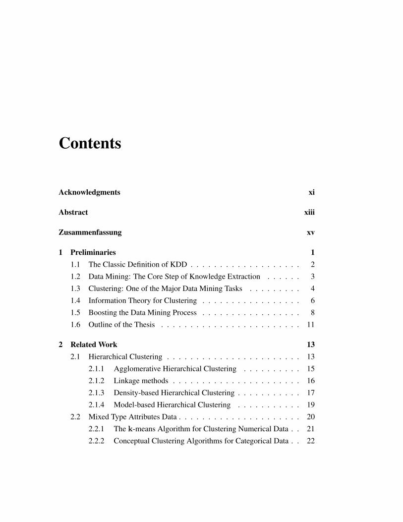
Figure 1.1: The KDD process.
1.1 The Classic Definition of KDD
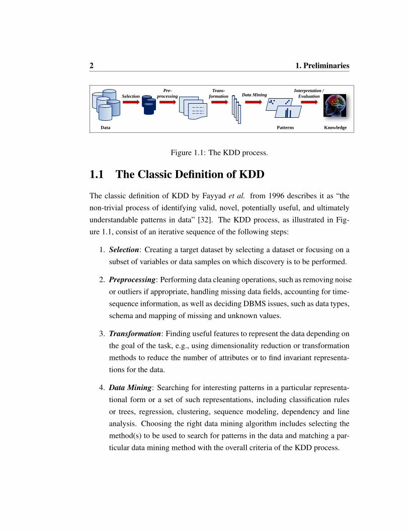
The classic definition of KDD by Fayyad et al. from 1996 describes it as “thenon-trivial process of identifying valid, novel, potentially useful, and ultimatelyunderstandable patterns in data” [32]. The KDD process, as illustrated in Fig-ure 1.1, consist of an iterative sequence of the following steps:
1. Selection: Creating a target dataset by selecting a dataset or focusing on asubset of variables or data samples on which discovery is to be performed.
2. Preprocessing: Performing data cleaning operations, such as removing noiseor outliers if appropriate, handling missing data fields, accounting for time-sequence information, as well as deciding DBMS issues, such as data types,schema and mapping of missing and unknown values.
3. Transformation: Finding useful features to represent the data depending onthe goal of the task, e.g., using dimensionality reduction or transformationmethods to reduce the number of attributes or to find invariant representa-tions for the data.
4. Data Mining: Searching for interesting patterns in a particular representa-tional form or a set of such representations, including classification rulesor trees, regression, clustering, sequence modeling, dependency and lineanalysis. Choosing the right data mining algorithm includes selecting themethod(s) to be used to search for patterns in the data and matching a par-ticular data mining method with the overall criteria of the KDD process.
1.2 Data Mining: The Core Step of Knowledge Extraction 3
5. Interpretation and Evaluation: Applying visualization and knowledge re-presentation techniques to the extracted patterns, and removing redundant orirrelevant patterns and translating the useful ones into terms understandableby users. The user may return to previous steps of the KDD process if theresults are unsatisfactory.
1.2 Data Mining: The Core Step of Knowledge Ex-traction
Since data mining is the core step of the KDD process, the terms KDD and Data
Mining are often used as synonyms. In [32], data mining is defined as a step inthe KDD process which consists of applying data analysis algorithms that, underacceptable computational efficiency limitations, produce a particular enumerationof patterns over the data.
In accordance with [44], existing data mining algorithms include the followingdata mining methods. Classification and prediction, clustering, outlier analysis,characterization and discrimination, frequent itemset and association rule mining,and evolution analysis. Classification and prediction are called supervised datamining tasks, because the goal is to learn a model for predicting a predefinedvariable. Supervised data mining requires that class labels are given for all dataobjects. The class label of an object assigns it to one of several predefined classes.The other techniques are called unsupervised, because the user does not previ-ously identify any of the variables to be learned. Instead, the algorithms have toautomatically identify any interesting regularities and patterns in the data. Clus-tering means grouping the data objects into classes by maximizing the similaritybetween objects of the same class and minimizing the similarity between objectsof different classes. We explain this important data mining task in detail in the fol-lowing section. Outlier analysis deals with the identification of data objects thatcannot be grouped in a given class or cluster, since they do not correspond to thegeneral model of the data. Characterization and discrimination provide the sum-

4 1. Preliminaries
marization and comparison of general features of objects. Frequent itemset andassociation rule mining focuses on discovering rules showing attribute value con-ditions that occur frequently together in a given dataset. And evolution analysismodels trends in time related data that evolve.
1.3 Clustering: One of the Major Data Mining Tasks
In this thesis, we mainly focus on clustering techniques w.r.t. the special chal-lenges posed by complex structured data. The goal of clustering is to find a naturalgrouping of a dataset such that data objects assigned to a common group calledcluster are as similar as possible and objects assigned to different clusters differ asmuch as possible. Consider for example the set of objects visualized in Figure 1.2.A natural grouping would assign the objects to two different clusters blue and red.Two outliers not fitting well to any of the clusters should be left unassigned.
Figure 1.2: Example for clustering consisting of two clusters blue and red andtwo outlier objects.
Cluster analysis has been used in a large variety of fields such as astronomy,physics, medicine, biology, archeology, geology, geography, psychology and mar-keting. Many different research areas contributed new approaches (namely patternrecognition, statistics, information retrieval, machine learning, bioinformatics anddata mining). In some cases, the goal of cluster analysis is a better understanding
1.3 Clustering: One of the Major Data Mining Tasks 5
Curvature
Labellum
Color
Length-Sepal(M)
CurvatureLabellum
Feature-Transformation
feature vector
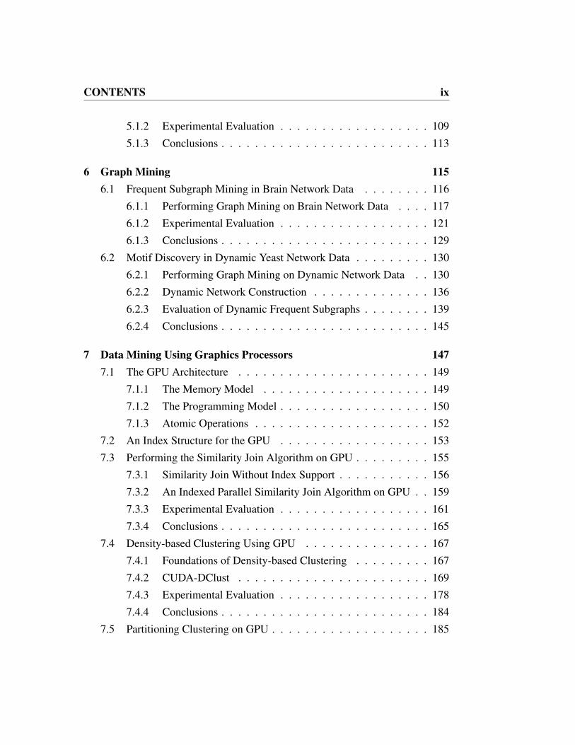
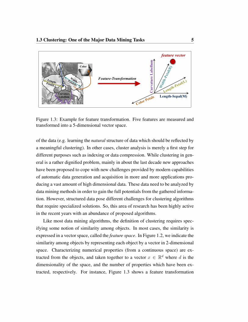
Figure 1.3: Example for feature transformation. Five features are measured andtransformed into a 5-dimensional vector space.
of the data (e.g. learning the natural structure of data which should be reflected bya meaningful clustering). In other cases, cluster analysis is merely a first step fordifferent purposes such as indexing or data compression. While clustering in gen-eral is a rather dignified problem, mainly in about the last decade new approacheshave been proposed to cope with new challenges provided by modern capabilitiesof automatic data generation and acquisition in more and more applications pro-ducing a vast amount of high dimensional data. These data need to be analyzed bydata mining methods in order to gain the full potentials from the gathered informa-tion. However, structured data pose different challenges for clustering algorithmsthat require specialized solutions. So, this area of research has been highly activein the recent years with an abundance of proposed algorithms.
Like most data mining algorithms, the definition of clustering requires spec-ifying some notion of similarity among objects. In most cases, the similarity isexpressed in a vector space, called the feature space. In Figure 1.2, we indicate thesimilarity among objects by representing each object by a vector in 2-dimensionalspace. Characterizing numerical properties (from a continuous space) are ex-tracted from the objects, and taken together to a vector x ∈ Rd where d is thedimensionality of the space, and the number of properties which have been ex-tracted, respectively. For instance, Figure 1.3 shows a feature transformation

6 1. Preliminaries
where the object is a certain kind of an orchid. The phenotype of orchids canbe characterized using the lengths and widths of the two petal and the three sepalleaves, of the form (curvature) of the labellum, and of the colors of the differentcompartments. In this example, five features are measured, and each object is thustransformed into a 5-dimensional vector space. To detect the similarity among twodata objects x and y represented as feature vectors, a metric distance function distis used. More specifically, let dist be one of the Lp norms, which is defined asfollows for an arbitrary p ∈ N.
dist(~x, ~y) = p
√√√√ d∑i=1
|xi − yi|p
Usually the Euclidean distance is used, i.e. p = 2. If we have more complex datatypes, we have to define a suited distance function.
For complex data objects, such as images, protein structures or text data, it isa non-trivial task to define domain specific distance functions. In Chapter 5, weintroduce SkyDist, a similarity measure for skyline objects. Skyline objects rep-resent a set of data objects that fit to a certain kind of query. The classic exampleis a user looking for cheap hotels which are close to the beach. Typically, it isunknown to the system how important the two conditions, distance and price,are to the user. The skyline query returns all offers which may be of interest. Thismeans, the skyline does not only contain the cheapest hotel and the hotel closestto the beach but also all hotels providing an outstanding combination of price anddistance, which makes them more attractive to the user than any other hotel inthe database. The high expressiveness of skylines aims at performing data miningon such data structures.
1.4 Information Theory for Clustering
Most clustering approaches suffer from a common problem: To obtain a goodresult, the user needs expertise about the data to select suitable parameters, e.g.

1.4 Information Theory for Clustering 7
the number of clusters, density thresholds or neighborhood sizes. In practice, thebest way to cope with this problem often is to run the algorithm several times withdifferent parameter settings. Thereby, suitable values for the parameters can belearned in a trial and error fashion. But it is obvious, that this is an extremely timeconsuming approach. And anyhow, it cannot guarantee that at least useful valuesfor the parameters are obtained.
A beneficial solution for that problem is to relate clustering to data compres-sion. Imagine you want to transfer a dataset consisting of feature vectors via anextremely expensive and small-banded communication channel from a sender toa receiver. Without clustering, each coordinate needs to be fully coded by trans-forming the numerical value into a bit string. But, if the data provides regularities,clustering can drastically reduce communication costs. For example a model-based clustering algorithm, like EM [27], can be applied to determine a statisticalmodel for the dataset, which defines more or less likely areas of the data space.With this knowledge, the data can be compressed very effectively since only thedeviations from the model need to be encoded which requires much less bits thanthe full coordinates. The model can be regarded as a codebook which allows thereceiver to de-compress the data again. Following the idea of (optimal) Huffmancoding, we assign few bits to points in areas of high probability and more bits toareas of low probability. The interesting observation is the following: the com-pression becomes the more effective, the better our statistical model fits to thedata.
This basic idea, often referred as the Minimum Description Length Principle(MDL) [40] allows comparing different clustering results: Assume we have twodifferent clusterings A and B of the same dataset. We can state that A is betterthan B if it allows compressing the dataset more effectively than B. Note that wehave to consider the overall communication costs, meaning that we have to addthe costs caused by the statistical model itself to the code length spent for the data.Thereby we achieve a natural balance between the complexity of the model andits fit to the data, and avoid the so-called over-fitting effect. Closely related ideas

8 1. Preliminaries
developed by different communities include the Bayesian Information Criterion(BIC), the Aikake Information Criterion (AIC) and the Information Bottleneckmethod (IB) [95].
In Chapter 3, we define a hierarchical variant of the MDL principle, calledhMDL. This novel criterion is able to assess a complete cluster hierarchy. Chap-ter 4 proposes iMDL, a coding scheme for performing integrative data mining ondata that consist of mixed type attributes.
1.5 Boosting the Data Mining Process
It has been shown that many data mining algorithms, including clustering, haveanother common problem besides the challenging parameterization. Most com-putations are extremely time consuming, particularly if they have to deal withlarge databases, which is a serious problem, as the amount of scientific data isapproximately doubling every year [92]. Typical algorithms for learning complexstatistical models from data are in quadratic or cubic complexity classes w.r.t. thenumber of objects and/or the dimensionality. To make these algorithms usable ina large and high dimensional database context is therefore an important goal.
One opportunity for boosting the data mining process is the intelligent adop-tion of graphics processing units (GPUs). GPUs have recently evolved from sim-ple devices for the display signal preparation into powerful coprocessors support-ing the CPU in various ways (cf. Figure 1.4). Graphics applications such asrealistic 3D games are computationally demanding and require a large number ofcomplex algebraic operations for each image update. Therefore, today’s graphicshardware contains a large number of programmable processors, which are opti-mized to cope with this high workload in a highly parallel way. Vendors of graph-ics hardware have anticipated that trend and developed libraries, precompilersand application programming interfaces. Most prominently, NVIDIA’s technol-ogy Compute Unified Device Architecture (CUDA) offers free development toolsfor the C programming language in which both the host program as well as the

1.5 Boosting the Data Mining Process 9
Figure 1.4: Growth trend of NVIDIA GPU vs. CPU (Source: NVIDIA).
kernel functions are assembled in a single program [1]. The host program or so-called main program is executed on the CPU. In contrast, the kernel functions areexecuted in a massively parallel fashion on hundreds of processors on the GPU.Analogous techniques are also offered by ATI using the brand names Close-to-Metal, Stream SDK, and Brook-GP.
In terms of peak performance, the GPU has outperformed state-of-the-art multi-core CPUs by a large margin. Hence, there is a great effort in many research com-munities such as life sciences [69, 73], mechanical simulation [94], cryptographiccomputing [8], machine learning [21], or even data mining [88] to use the com-putational capabilities of GPUs even for purposes which are not at all related tocomputer graphics. The corresponding research area is called General Processing-Graphics Processing Units (GP-GPU). We focus on exploiting the computationalpower of GPUs for data mining. Therefor specialized indexing methods are re-quired because of the highly parallel but restricted programming environment. Inthis thesis, we propose a multi-dimensional indexing method that is well suitedfor the architecture provided by the GPU.

10 1. Preliminaries
To demonstrate that highly complex data mining tasks can be efficiently imple-mented using novel parallel algorithms, we propose parallel versions of generalsimilarity search and two widespread clustering algorithms in Chapter 7. Thesealgorithms make use of the high computational power provided by the GPU. Theyare highly parallel and exploit thus the high number of simple SIMD (Single In-struction Multiple Data) processors of today’s graphics hardware. The paralleliza-tion which is required for GPUs differs considerably from previous parallel algo-rithms which have focused on shared-nothing parallel architectures prevalent inserver farms. For even further accelerations, we propose the indexed variants ofthese algorithms.
1.6 Outline of the Thesis 11
1.6 Outline of the Thesis
In this thesis, we aim at discovering novel data mining algorithms for mining dif-ferent kinds of data structures. In addition, we focus on boosting opportunities forcomputationally intensive steps of the data mining process. The detailed outlineis given in the following.
In Chapter 1, we give the reader a short introduction to the broader context of thisthesis. In Chapter 2, we provide a brief overview of traditional data mining algo-rithms on structured data and present a rather general survey on advanced cluster-ing methods. In addition, we introduce the broad related work on techniques forboosting the data mining process by an intelligent adoption of Graphics Process-ing Units (GPUs).
Chapter 3 to Chapter 6 deal with advanced data mining algorithms on structureddata types. Here we focus on hierarchical data mining, the analysis of more com-plex data types like mixed type attribute data and skyline objects, and graph min-ing. In Chapter 3, we present the two hierarchical clustering algorithms ITCH(Information-Theoretic Cluster Hierarchies) and GACH (Genetic Algorithm forfinding Cluster Hierarchies). ITCH, is an EM-based clustering approach to ar-range only natural, valid, and meaningful clusters in a hierarchy guided by theidea of data compression. GACH overcomes the common problem of gettingstuck in a local optimum by a beneficial combination of genetic algorithms, infor-mation theory and model-based clustering. The ideas on hierarchical data mininghave already been published by the author [12]. In Chapter 4, we propose INTE-GRATE [13], a new algorithm for performing integrative parameter-free cluster-ing of data with mixed type attributes. Chapter 5 provides SkyDist [17], a novelsimilarity measure for the comparison of different skyline objects. Chapter 6 isdedicated to our novel approaches that have the ability to detect patterns in static aswell as in dynamic networks. We published a large case-study on static brain net-work models [78, 99] and our work on finding frequent dynamic subgraphs [100].

12 1. Preliminaries
Chapter 7 presents our work on data mining using GPUs. Section 7.1 explainsthe graphics hardware and the CUDA programming model underlying our pro-cedures. In Section 7.2, we develop a multi-dimensional index structure for si-milarity queries on the GPU that can be used for further accelerations of the datamining process. Section 7.3 presents non-indexed as well as indexed algorithmsto perform the similarity join on graphics hardware. Section 7.4 and Section 7.5are dedicated to GPU-capable algorithms for density-based and partitioning clus-tering. The contributions on data mining using GPUs have already been publishedby the author in two publications [15, 14].
Chapter 8 summarizes and discusses the major contributions of this thesis. Itincludes some ideas for future directions.

Chapter 2
Related Work
To survey the large work on performing data mining of structured data, we mainlyfocus on well-known clustering techniques for hierarchical data in Section 2.1 aswell as for mixed type attributes data in Section 2.2. In Section 2.3, we describesome ideas of how to enhance the effectiveness of many data mining concepts byinformation theory. In the field of graph mining, we present different algorithmsfor finding interesting patterns, i.e. frequent subgraphs in one large network or ina given set of networks (cf. Section 2.4). Finally, we conclude the related researchon acceleration opportunities for the data mining process by the use of graphicsprocessors.
2.1 Hierarchical Clustering
Hierarchical clustering algorithms compute a hierarchical decomposition of thedataset instead of a unique assignment of data objects to clusters in partitioningclustering. Given a dataset DS, the goal is to produce a hierarchy, which is vi-sualized as a tree, called dendrogram. The nodes of the dendrogram representsubsets of DS simulating the structure found in DS with the following properties(cf. Figure 2.1):

14 2. Related Work
Figure 2.1: The hierarchical structure, present in the dataset on the left side, isvisualized by the dendrogram on the right side.
• The root of the dendrogram represents the whole dataset DS.
• Each leaf of the dendrogram corresponds to one data object of DS.
• The internal nodes of the dendrogram are defined as the union of their chil-dren, i.e., each node represents a cluster containing all objects in the corre-sponding subtree.
• Each level of the dendrogram represents a partition of the dataset into dis-tinct clusters.
Hierarchical clustering can be subdivided into agglomerative methods, which pro-ceed by series of fusions of data objects into clusters, and divisive methods, whichseparate the data objects successively into finer clusters. Agglomerative hierar-chical clustering algorithms follow a bottom-up strategy by merging the clustersiteratively. They start by placing each data object in its own single cluster. Then,the clusters are merged together into larger clusters by grouping similar data ob-jects together until the entire dataset is encapsulated into one final root cluster.

2.1 Hierarchical Clustering 15
Most hierarchical methods belong to this category. They differ only in their defi-nition of between-cluster similarity.
Divisive hierarchical clustering works in the opposite way - it starts with alldata objects in one root cluster and subdivides them into smaller clusters untileach cluster consists of only one single data object. Divisive methods are notgenerally available, and have been rarely applied. The reason for this is mainlycomputational - divisive clustering is more computationally expensive when itcomes to making decisions in dividing a cluster in two clusters given all possiblechoices. While in agglomerative procedures in one step two out of maximumn elements have to be chosen for merging, in divisive procedures fundamentallyall subsets have to be analyzed so that divisive procedures have an algorithmiccomplexity of O(2n).
2.1.1 Agglomerative Hierarchical Clustering
Given a dataset DS of n objects, the basic process of agglomerative hierarchicalclustering is defined as follows:
1. Place each data object xi ∈ DS (i = 1, . . . n) in one single cluster Ci.Create the list of initial clusters C = C1, . . . , Cn, which will build the leavesof the resulting dendrogram.
2. Find the two clusters Ci, Cj ∈ C with the minimum distance to each other.
3. Merge the clusters Ci and Cj to create a new internal node Cij which willbe the parent of Ci and Cj in the resulting dendrogram. Remove Ci and Cjfrom C.
4. Repeat step (2) and (3) until the total number of clusters in C becomes one.
In the first step of the algorithm, when each object represents its own cluster, thedistances between the clusters are defined by the chosen distance function be-tween the objects of the dataset. However, once several objects have been linked
16 2. Related Work
together, a linkage rule is needed to determine the actual distance between twoclusters. There are numerous linkage rules that have been proposed. In the fol-lowing, some of the most commonly used are presented.
2.1.2 Linkage methods
Let DS be a dataset, dist denotes the distance function between the data objectsof DS, and let Ci and Cj be two disjunct clusters consisting of objects of DS, i.e.Ci, Cj ⊆ DS and Ci ∩ Cj = ∅. In the following, some of the most commonlyused linkage rules to determine the distance between two clusters are described.
Single Link
One of the most widespread approaches to agglomerative hierarchical clusteringis Single Link [72]. Single Link defines the distance distSL between any twoclusters Ci and Cj as the minimum distance between them, i.e. as the distancebetween the two closest objects:
distSL(Ci, Cj) = minxi∈Ci,xj∈Cj
{dist(xi, xj)}.
Using the Single Link method often causes the chaining phenomenon, also calledSingle Link effect, which is a direct consequence of the Single Link approachtending to build a chain of objects that connects two clusters.
Complete Link
The Complete Link method [25] is the opposite of Single Link. Complete Linkdefines the distance distCL between any two clusters Ci and Cj as the maximumdistance between them:
distCL(Ci, Cj) = maxxi∈Ci,xj∈Cj
{dist(xi, xj)}.
2.1 Hierarchical Clustering 17
This method should not be used if there is a lot of noise expected to be present inthe dataset. It also produces very compact clusters. This method is useful if one isexpecting objects of the same cluster to be far apart in multi-dimensional space.In other words, outliers are given more weight in the cluster decision.
Average Link
Average Link [98] calculates the mean distance between all possible pairs of ob-jects belonging to the two clusters Ci and Cj . Hence, it is computationally moreexpensive to compute the distance distAV G than the aforementioned methods:
distAV G(Ci, Cj) =1
|Ci| · |Cj|∑
xi∈Ci,xj∈Cj
{dist(xi, xj)}.
Average Link is sometimes also referred to as UPGMA (Unweighted Pair-GroupMethod using Arithmetic averages). There are several other variations of thismethod, e.g. Weighted Pair-Group Average, Unweighted Pair-Group Centroid,Weighted Pair-Group Centroid, but one should understand that it is a tradeoffbetween Single Link and Complete Link.
2.1.3 Density-based Hierarchical Clustering
The algorithm OPTICS (Ordering Points To Identify the Clustering Structure) [4]avoids the Single Link effect by requiring a minimum object density per cluster,i.e. MinPts number of objects are within a hypersphere with radius ε. The mainidea of OPTICS is to compute a complex hierarchical cluster structure, i.e. all pos-sible clusterings with the parameter ε ranging from 0 to a given maximum valuesimultaneously during a single traversal of the dataset. The resulting cluster struc-ture is visualized by a so-called reachability plot where the objects are plottedaccording to the sequence specified in the cluster ordering along the x-axis, andfor each object, its corresponding distance along the y-axis. Figure 2.2 depicts thereachability plot based on the cluster ordering computed by OPTICS for a given

18 2. Related Work
ε1
ε2
B
B
A1 A2
A
Figure 2.2: The reachability plot computed by OPTICS for a given sample 2-dimensional dataset.
sample 2-dimensional dataset. Valleys in this plot indicate clusters: objects hav-ing a small reachability value are closer and thus more similar to their predecessorobjects than objects having a higher reachability value. The reachability plot gen-erated by OPTICS can be cut at any level ε′ parallel to the x-axis. It representsthe partitioning according to the density threshold ε′. A consecutive subsequenceof objects having a smaller reachability value than ε′ belongs to the same clusterthen. Referring to the given example in Figure 2.2, a cut at the level ε1 results intwo clusters A and B. Compared to this clustering, a cut at level ε2 would yieldthree clusters. The cluster A is split into two smaller clusters denoted by A1 andA2 and cluster B decreased its size. This illustrates, how the hierarchical clusterstructure of a dataset is revealed at a glance and can be easily explored by visualinspection.
Single Link is a special case of OPTICS (whereMinPts = 1 and a maximumvalue of ε =∞). In this case, OPTICS has the same drawbacks like Single Link,i.e. missing stability w.r.t. noise objects and the Single Link effect. OPTICSovercomes this drawback if MinPts is set to higher values.
2.1 Hierarchical Clustering 19
2.1.4 Model-based Hierarchical Clustering
For many applications and further data mining steps, it is essential to have a modelof the data. Hence, clustering with PDFs, which goes back to the popular EM al-gorithm [27], is a widespread approach for performing clustering. EM is a gener-alization of the k-means algorithm, a partitioning clustering algorithm for numeri-cal data (cf. Section 2.2.1). After a suitable initialization, EM iteratively optimizesa mixture model of k Gaussian distributions until no further significant improve-ment of the log-likelihood of the data can be achieved. In detail, we generate adataset that consists of first picking a centroid at random and then adding somenoise. If the noise is normally distributed, this procedure will result in clustersof spherical shape. Model-based clustering assumes that the data were generatedby a model and tries to recover the original model from the data. More precisely,the data has been generated from a finite mixture of k distributions, but that thecluster membership of each data point is not observed. In EM, the log-likelihoodis used to calculate the model parameters θ:
L(θ) = logn∏i=1
P (xi|θ) =n∑i=1
logP (xi|θ)
Model-based clustering aims for determine the parameter θ that maximizes thelog-likelihood:
L(θ) = maxθL(θ) = max
θ
n∑i=1
logP (xi|θ)
In the case of k clusters a vector ~θ = {θ1, · · · , θk} has to be optimized:
L(~θ) =n∑i=1
logP (xi|~θ) =n∑i=1
k∑j=1
logWj + logP (xi|θj)
,
where Wj is the weight of the cluster that represents the number of objects asso-ciated to that cluster.

20 2. Related Work
EM can be applied to many different types of probabilistic modeling. In casethe probability density function (PDF) which is associated to a cluster C is amultivariate Gaussian in a d-dimensional space which is defined by the parametersµC and ΣC (where µC = (µC,1, ..., µC,d)
T is a vector from a d-dimensional space,called the location parameter, and ΣC is a d× d covariance matrix), the definitionof P (x|θ) is as follows:
P (x|µC ,ΣC , x) =1√
(2π)d · |ΣC |· e−
12
(x−µC)T·Σ−1C ·(x−µC).
The EM algorithm is an iterative procedure where in each iteration step the mix-ture model of the k distributions are optimized until no further significant im-provement of the log-likelihood of the data can be achieved. Usually, a very fastconvergence of EM is observed. However, the algorithm may get stuck in localmaximum of the log-likelihood. Moreover, the quality of the clustering resultstrongly depends on an appropriate choice of k, which is a non-trivial task in mostapplications.
A hierarchical extension of the EM algorithm was presented by Vasconcelosand Lippman in 1998 [97]. The efficiency of this approach is achieved by pro-gressing the data in a bottom-up fashion, i.e. the mixture components of a givenlevel are clustered to retrieve those components of the level above. This procedurerequires only knowledge of the mixture parameters, the intermediate samples donot have to be resorted. With regards to practical applications, this algorithm leadsto computationally efficient methods for estimating density hierarchies capable ofdescribing data at different resolutions.
2.2 Mixed Type Attributes Data
A prominent characteristic of data mining is that it deals with very large and com-plex datasets. These data often contain millions of objects described by varioustypes of attributes or variables, e.g. numerical, categorical, ratio or binary. Hence,

2.2 Mixed Type Attributes Data 21
integrative data mining algorithms have to be scalable and capable of dealing withdifferent types of attributes. In terms of clustering, we are interested in algo-rithms which can efficiently cluster large datasets containing both numeric andcategorical values because such datasets are frequently encountered in data min-ing applications. The traditional way to treat categorical attributes as numericdoes not always produce meaningful results because many categorical domainsare not ordered.
One simple idea for performing integrative clustering on heterogeneous datais to combine k-means based methods with the k-modes algorithm. The algorithmk-prototypes derives advantage from this combination, and is therefore one of thefirst approaches towards integrative clustering.
2.2.1 The k-means Algorithm for Clustering Numerical Data
The k-means algorithm [72] is one of the mostly used partitioning non-hierarchicalclustering approach. The procedure follows a simple and easy way to group agiven datasetDS consisting of n numeric objects into a certain number of k (< n)clusters. First, k centroids are defined, one for each cluster. Then, the algorithmtakes each point of DS and associates it to the nearest centroid, until no morepoint is pending. Afterwards, the k new centroids (the mean value µ over thecoordinates of all data points belonging to the specific cluster) are recalculated,and thus, a new association has to be determined between the points of DS andthe nearest new centroid. These two steps are performed until no more locationchanges of the centroids are observed. Finally, k-means aims at minimizing anobjective function, in this case the within clusters sum of squared errors (WCSS).
WCSS =k∑j=1
n∑i=1
(dist(xi,j, µj))2,
where dist(xi,j, µj) is a chosen distance function between a data point xi,j and thecentroid µj of cluster Cj , is an indicator of the distance of the n data points fromtheir respective cluster centers.

22 2. Related Work
The main advantage of k-means is its efficiency. It can be proven that convergenceis reached in O(n) iterations. However, this method has four major drawbacks:First, the number of clusters k has to be specified in advance, second, the clus-ter compactness measure WCSS and thus the clustering result is very sensitive tonoise and outliers. In addition, k-means implicitly assumes a Gaussian data dis-tribution, and is thus restricted to detect spherically compact clusters. The majordrawback lies in its limited practicability to numeric data.
2.2.2 Conceptual Clustering Algorithms for Categorical Data
In principle the formulation of the WCSS in Section 2.2.1 is also valid for cate-gorical and mixed type objects. The reason why the k-means algorithm cannotcluster categorical objects is that the calculation of the mean value is not definedfor categorical data. These limitations can be removed by the following modifica-tions:
• Use a simple matching distance function for categorical objects.
• Replace means as cluster representatives by modes.
• Use a frequency-based method to find the modes.
A Distance Function for Categorical Objects
Let x, y be two categorical objects described by m categorical attributes. The dis-tance function between these two objects can be defined by the total mismatchesof the corresponding attribute categories of the two objects. The smaller the num-ber of mismatches is, the more similar x and y. This measure is often referred toas simple matching [56]. Formally this distance function is defined as follows:
distSimple(x, y) =m∑i=1
δ(xi, yi), where δ(xi, yi) =
0, if xi = yi,
1, if xi 6= yi.

2.2 Mixed Type Attributes Data 23
Modes as Cluster Representatives
Consider a set of n categorical objects X described by categorical attributes,A1, A2, · · · , Am. The mode of this set is an array q = [q1, q2, · · · qm] of lengthm that minimizes the following formula:
D(X, q) =n∑i=1
distSimple(Xi, q)
Calculation of the Modes
Let nck,i be the number of objects having the k-th category ck,i in attribute Ai,and let p(Ai = ck,i|X) be the relative frequency of category ck,i in X . Then thefunction D(X, q) is minimized if and only if p(Ai = qi|X) ≥ p(Ai = ck,i|X) forqi 6= ck,i for all i ∈ {1, · · · ,m}[48].
This theorem defines a way to find the mode q from a given set of categoricalobjects X , and therefore it is important because it allows the k-means paradigmto be used to cluster categorical data.
The Algorithm k-modes
Conceptual clustering algorithms, like k-modes [49] implement the idea of clus-tering categorical data by using distSimple as distance function and by means ofthe aforementioned modifications of k-means clustering. The procedure of thealgorithm k-modes can be summarized as follows:
1. Select k initial modes, one for each cluster.
2. Allocate an object to the cluster whose mode is the nearest to it accordingto the distance function distSimple; update the mode of the cluster after eachallocation according to the theorem presented in Section 2.2.2.
3. After all objects have been allocated to clusters, retest the distance of objectsagainst the current modes. If an object is found such that its nearest mode

24 2. Related Work
belongs to another cluster rather than its current one, reallocate the objectto that cluster and update the modes of both clusters.
4. Repeat step (3) until no object has changed clusters after a full cycle test ofthe whole dataset.
Like the k-means algorithm, the k-modes algorithm also produces locally optimalsolutions that are dependent on the initial modes and the order of objects in thedataset. Its efficiency relies on good search strategies. For data mining problems,which often involve many concepts and very large object spaces, the conceptsbased search methods can become a potential handicap for these algorithms todeal with extremely large datasets.
2.2.3 The k-prototypes Algorithm for Integrative Clustering
One of the first algorithms for integrative clustering is k-prototypes [47]. The dis-tance between two mixed type objects x and y, which are described bym attributesAn1 , A
n2 , · · · , Anp , Acp+1, A
cp+2, · · · , Acm is measured by the following formula:
distMixed =
p∑i=1
(xi − yi)2 + γm∑
i=p+1
δ(xi, yi).
The first term is the squared Euclidean distance measure on the p numeric at-tributes Ani and the second term is the simple matching distance function on them−p categorical attributes Aci . The weight γ is used to avoid favoring either typeof attribute. The influence of this parameter in the clustering process is discussedin the publication by Huang [47].
2.3 Information Theory in the Field of Clustering
Many clustering algorithms suffer from the problem that they require a difficultparameter setting. Hence, several advanced clustering approaches directly focus
2.3 Information Theory in the Field of Clustering 25
on parameter-free partitioning clustering and are based on the Akaike InformationCriterion (AIC), the Bayesian Information Criterion (BIC) and Minimum Descrip-tion Length (MDL) [40]. For these methods, the data itself is the only source ofknowledge. Information theoretic arguments are applied for model selection dur-ing clustering, and these approaches involve a lossless compression of the data.
The work of Still and Bialek [91] provides important theoretical background byusing information-theoretic arguments to relate the maximum number of clustersthat can be detected by partitioning clustering with the size of the dataset. Thealgorithm X-Means [81] combines the k-means paradigm with BIC for parameter-free clustering. X-Means involves an efficient top-down splitting algorithm whereintermediate results are obtained by bisecting k-means and are evaluated withBIC. However, only spherically Gaussian clusters can be detected. The algorithmG-means (Gaussian means) introduced in [43] has been designed for parameter-free correlation clustering. G-means follows a similar algorithmic paradigm asX-Means with top-down splitting and the application of bisecting k-means uponeach split. However, the criterion to decide whether a cluster should be split upinto two is based on a statistical test for Gaussianity. Splitting continues untilthe clusters are Gaussian, which implies of course, that non-Gaussian clusters canstill not be detected. The algorithm PG-means (Projected Gaussian means) byFeng and Hamerly [33] is similar to G-means but learns models with increasingk with the EM algorithm. In each iteration, various 1-dimensional projections ofthe data and the model are tested for Gaussianity. Experiments demonstrate thatPG-means is less prone to over-fitting than G-means.
It turns out that the underlying clustering algorithm and the choice of the sim-ilarity measure are already some kind of parameterization which implicitly comeswith specific assumptions. The commonly used Euclidean distance e.g. assumesGaussian data. In addition, the algorithms discussed so far are very sensitive w.r.t.noise objects or outliers. These problems are addressed by the recently proposedalgorithm RIC (Robust Information-theoretic Clustering) by Bohm et al. [10].This algorithm can be applied for post-processing an arbitrary imperfect initial

26 2. Related Work
pdfLapl(μ=3.5 σ=1)(x)
5 % 4.3 Bit
pdfGauss(μ=3.5 σ=1)(y)
x
Figure 2.3: Coding scheme for cluster objects of the RIC algorithm. In additionto the data, type and parameters of the PDF need to be coded for each cluster.
clustering. It is based on MDL and introduces a coding scheme especially suit-able for clustering together with algorithms for purifying the initial clusters fromnoise. In a first step, RIC removes noise objects from the initial clusters, and thenmerges clusters if this allows for more effective data compression. The algorithmoperates with arbitrary data distributions, taken from a fixed set of PDFs.
The coding scheme for a data point p of a cluster C is illustrated in Figure 2.3.Here, we have a Laplacian distribution for the x-coordinate and a Gaussian dis-tribution for the y-coordinate. Both distributions are assumed with µ = 3.5 andσ = 1. We need to assign code patterns to the coordinate values such that co-ordinate values with a high probability (such as 3 < x < 4) are assigned shortpatterns, and coordinate values with a low probability (such as y = 12 to give

2.4 Graph-structured Data 27
a more extreme example) are assigned longer patterns. Provided that a coordi-nate is really distributed according to the assumed distribution function, Huffmancodes optimize the overall compression of the dataset. Huffman codes associatea bit string of length l = log2(1/p(pi)) to each coordinate pi, where p(pi) is theprobability of the (discretized) coordinate value.
The algorithm OCI (Outlier-robust Clustering using Independent Components) [11]provides parameter-free clustering of noisy data and allows detecting non-Gaussianclusters with non-orthogonal major directions. Technically this is achieved bydefining a very general cluster notion based on the Exponential Power Distribution(EPD) and by integrating Independent Component Analysis (ICA) into clustering.The EPD includes a wide range of symmetric distribution functions, e.g. Gaus-sian, Laplacian and uniform distributions and an infinite number of hybrid types inbetween by an additional shape parameter. Beyond correlations detected by Prin-cipal Component Analysis (PCA), which correspond to correlation clusters withorthogonal major directions, ICA allows to detect general statistical dependenciesin the data.
2.4 Graph-structured Data
In this section, we review the previous work on finding patterns in graph data andfocus on three problems. First, frequent subgraphs across a dataset of graphs. Sec-ond, frequent subgraphs within one single large graph. Third, frequent subgraphsin dynamic graph data.
2.4.1 Graph Dataset Mining
The graph dataset mining approaches can be broadly divided into two classes,apriori-based and pattern-growth based. AGM (Apriori-based Graph Mining) [52]determines subgraphs s in a dataset DS of labeled graphs that occur in at least tpercentage of all graphs (also called transactions) in DS. AGM uses a canonical

28 2. Related Work
X
YZ
Xba
a b
v0
v1
v2 v3
X
YZ
Xba
a b
v0
v1
X
YZ
Xba
a b
v0
v1
backward extension forward extension
v2 v3 v2 v3
Figure 2.4: Illustration of the rightmost extension used in gSpan.
representation of subgraphs in order to reduce runtime costs for subgraph isomor-phism checking.
Similar to AGM, FSG (Frequent SubGraph Discovery) [61] uses a canonicallabeling based on the adjacency matrix. Canonical labeling, candidate generationand evaluation are sped up in FSG using graph invariants and the TransactionID principle, which stores the ID of transactions a subgraph appeared in. Thisspeed-up is paid for by reducing the class of subgraphs discovered to connectedsubgraphs, i.e. subgraphs where a path exists between all pairs of nodes.
The most well-known member of the class of pattern-growth algorithms, gSpan(graph-based Substructure pattern mining) [107], discovers frequent substructuresefficiently without candidate generation. It is built on depth first search (DFS) tree.Given a graph S with nodes N and edges E, and a DFS tree TR, we call the start-ing node in TR, v0, the root, and the last visited node, vn, the rightmost node. Thestraight path from v0 to vn is called the rightmost path. Figure 2.4 shows an exam-ple. The red edges form a DFS tree. The nodes are discovered in the order v0, v1,v2, v3. The node v3 is the rightmost node. The rightmost path is v0 → v1 → v3.
The new method, called rightmost extension, restricts the extension of newedges in a graph as follows: Given a graph S and a DFS tree TR, a new edge ecan be added between the rightmost node and other nodes on the rightmost path(backward extension) or it can introduce a new node and connect it to nodes on the

2.4 Graph-structured Data 29
rightmost path (forward extension). If we want to extend the graph in Figure 2.4,the backward extension candidate can be (v3, v0). The forward extension candi-dates can be edges extending from v3, v1 or v0 with a new node inserted. Sincethere could be multiple DFS trees for one graph, gSpan establishes a set of rules toselect one of them as representative so that the backward and forward extensionswill only take place on one DFS tree.
Overall, new edges are only added to the nodes along the rightmost path. Withthis restricted extension, gSpan reduces the generation of the same graphs, anddefines a canonical form of S. However, it still guarantees the completeness ofenumerating all frequent subgraphs.
2.4.2 Large Graph Mining
Unlike graph dataset mining, large graph mining intends to find subgraphs thathave at least t embeddings in one large graph. Note that any large graph min-ing algorithm can be applied to the graph dataset mining problem as well, simplyby concatenation of all single graphs from a dataset into one large graph. Ofcourse, subgraphs that include nodes from distinct single graphs must be prunedduring pattern search. The reverse, applying graph dataset mining algorithms tolarge graphs, is not directly possible. GREW [63] and SUBDUE [23] are greedyheuristic approaches for frequent graph mining that deal speed for completenessof the solution. GREW iteratively joins frequent pairs of nodes (i.e. edges) intoone supernode and determines disjoint embeddings of connected subgraphs by amaximal independent set algorithm. GREW maintains the location of the em-beddings of the previously identified frequent subgraphs by rewriting the inputgraph, and therefore it is also applicable on very large graph datasets. This con-cept of edge contraction and graph rewriting is basically similar to that used byother heuristic algorithms, e.g. SUBDUE. However, GREW substantially extendsthis idea in multiple ways: First, it allows the concurrent contraction of differentedge types, and second, GREW employs a set of heuristics in order to find longerand denser frequent patterns. Hence, this algorithm is enabled to simultaneously
30 2. Related Work
discover multiple patterns and to find longer patterns in fewer iterations. Finally,GREW uses a representation of the rewritten graph that retains all the informationpresent in the original graph, and thus it precisely identifies whether or not thereis an embedding of a particular subgraph. This result guarantees a lower boundon the frequency of each discovered pattern. SUBDUE tries to minimize the min-imum description length (MDL) of a graph by compressing frequent subgraphs.Frequent subgraphs are replaced by one single node and the MDL of the remain-ing graph is then determined. Those subgraphs whose compression minimizes theMDL are considered frequent patterns in the input graph. The candidate graphsare generated starting from single nodes to subgraphs with several nodes, using acomputationally constrained beam search.
Similarly, vSIGRAM and hSIGRAM [62] find subgraphs that are frequentlyembedded within a large sparse graph, using “horizontal” breadth-first search and“vertical” depth-first search, respectively. They employ efficient algorithms forcandidate generation and candidate evaluation that exploit the sparseness of thegraph.
While most of the techniques mentioned before often use some sort of heuris-tic search strategy that repeatedly compresses the graph to find frequent sub-graphs, methods based on sampling subgraphs to estimate their frequency are pre-dominant in application domains, like bioinformatics [55, 102]. Another strategyis to exhaustively enumerate all subgraphs. This has the advantage that one canthen compute exact rather than approximate frequencies, but for large graphs, it isonly feasible for subgraphs with a limited number k of nodes, typically k ∈ {3, 4}.
2.4.3 Dynamic Graph Mining
While the evolution of graphs over time has been addressed before, the corre-sponding studies predominantly dealt with topics such as densification and shrink-ing diameters of real-world graphs over time [65]. Only a few papers [18, 29, 64]define terminology for mining dynamic networks, but to the best of our knowledgeno paper presents an efficient algorithm for detecting frequent subgraphs within

2.5 Boosting Data Mining 31
dynamic graphs so far.
2.5 Boosting Data Mining
In this section, we survey the related research in general purpose computationsusing Graphics Processing Units (GPUs) with particular focus on database man-agement and data mining.
Figure 2.5: The NVIDIA GeForce 8800 GTX graphics processor (Source:NVIDIA).
2.5.1 General Processing-Graphics Processing Units
Theoretically, GPUs are capable of performing any computation that can be trans-formed to the model of parallelism and that allow for the specific architecture ofthe GPU. This model has been exploited for multiple research areas. One scien-tific publication on computations from the field of life sciences has been publishedby Manavski and Valle [73]. The authors propose an extremely fast solution of theSmith-Waterman algorithm, a procedure for searching for similarities in protein

32 2. Related Work
and DNA databases, running on GPU and implemented in the CUDA program-ming environment. This algorithm launches a great number of parallel threadssimultaneously to fully exploit the huge computational power of the GPU. It pur-sues the strategy that each GPU thread computes the whole alignment of the querysequence with one database sequence. All threads are grouped in a grid of blockswhen running on the graphics card. In order to make the most efficient use ofthe GPU resources the computing time of all threads in the same grid must be asnear as possible. For this reason, the sequences of the database are pre-orderedw.r.t. their length. Hence, all adjacent threads align the query sequence with twodatabase queries having the nearest possible sizes.
Another widespread application area that uses the processing power of theGPU is mechanical simulation. One example is the work by Tascora et al. [94],that presents a novel method for solving large cone complementarity problems bymeans of a fixed-point iteration algorithm, in the context of simulating the fric-tional contact dynamics of large systems of rigid bodies. The proposed algorithmis well suited for running on parallel platforms that support the single instructionmultiple data (SIMD) computational paradigm, which is ideally suited for han-dling problems with contacts in excess of hundreds of thousand.
To demonstrate the nearly boundless possibilities of performing computationson the GPU, we introduce one more example, namely cryptographic comput-ing [8]. In this paper, the authors present a record-breaking performance for theElliptic Curve Method (ECM) of integer factorization. This approach uses the par-allelism of the GPU to handle several curves for a given auxiliary integer, whichcan thus be stored in the shared memory of a multiprocessor. All processors inone multiprocessor follow the same series of instructions which is a scalar multi-plication on the respective curve modulo the same parameterm and with the samescalar s. The authors achieve an extreme speedup that results of extra hardwareusing the novel ECM implementation.

2.5 Boosting Data Mining 33
2.5.2 Database Management Using GPUs
Some research papers propose techniques to speed up relational database oper-ations on GPU. Two recent papers [67, 16] address the topic of similarity joinin feature space which determines all pairs of objects from two different sets Rand S fulfilling a certain join predicate. The most common join predicate is theεSJ -join which determines all pairs of objects having a distance of less than apredefined threshold εSJ . The authors of [67] propose an algorithm based on theconcept of space filling curves, e.g. the z-order, for pruning the search space, run-ning on an NVIDIA GeForce 8800 GTX using the CUDA toolkit. The z-orderof a set of objects can be determined very efficiently on GPU by highly paral-lelized sorting. Their algorithm operates on a set of z-lists of different granularityfor efficient pruning. However, since all dimensions are treated equally, perfor-mance degrades in higher dimensions. An approach that overcomes that kind ofproblem is presented in [16]. Here, the authors parallelize the baseline techniqueunderlying any join operation with an arbitrary join predicate, namely the nestedloop join (NLJ), a powerful database primitive that can be used to support manyapplications including data mining.
Govindaraju et al. [38, 39] demonstrate that important building blocks forquery processing in databases, e.g. sorting, conjunctive selections, aggregations,and semi-linear queries can be significantly speed up by the use of GPUs. Theiralgorithm GPUTeraSort uses the GPU as a co-processor to sort databases with bil-lions of records. GPUTeraSort is general and can handle long records with widekeys. This hybrid sorting architecture offloads compute- and memory-intensivetasks to the GPU to achieve higher I/O performance and better main memoryperformance. A bitonic sorting network is mapped to GPU rasterization oper-ations and uses the GPUs programmable hardware and high bandwidth memoryinterface. This novel data representation improves GPU cache efficiency and min-imizes data transfers between the CPU and the GPU.
34 2. Related Work
2.5.3 Data Mining Using GPUs
Finally, we survey some recent approaches for data mining using the GPU. In [20]a parallelized clustering approach for graphics hardware is presented. This algo-rithm extends the basic idea of k-means clustering by calculating the distancesfrom a single input centroid to all objects at one time that can be done simulta-neously in hardware. Thus the authors are able to exploit the high computationalpower and pipeline of GPUs, especially for core operations, like distance com-putations and comparisons. An additional efficient method that is designed toexecute clustering on data streams confirms a wide practical field of clustering onGPU.
The algorithm k-means was also parallelized by Shalom et al. [87]. In theirimplementation multi-pass rendering and multi shader program constants are used.This is done by minimizing the use of GPU shader constants, which leads toa significant improvement of the performance as well as to a reduction of thedata transactions between the CPU and the GPU. Handling data transfers betweenthe necessary textures within the GPU is much more efficient than using shaderconstants. This is mainly due to the high memory bandwidth available in theGPU pipeline. Since all the steps of the k-means algorithm are able to be imple-mented in the GPU, the transferring of data back to the CPU during the iterationsis avoided. The programmable capabilities of the GPU have been thus exploitedto efficiently implement k-means clustering in the GPU.
Another approach implemented hierarchical agglomerative clustering basedon complete linkage and the single linkage methods for the use in GPU [88]. Thecomputations of distances and centroids, as well as the update operation of thesimilarity matrix is performed in parallel on the Graphics processor. To processthe complete similarity matrix, n × n/2 threads are needed, as this refers to thesize of the matrix for a dataset consisting of n data objects. Compared to theconventional CPU implementation, this approach achieves a speedup factor ofabout 15 to 90.

Chapter 3
Hierarchical Data Mining
Since dendrograms and similar hierarchical representations provide extremelyuseful insights into the structure of a dataset, hierarchical clustering has becomevery popular in various scientific disciplines, such as molecular biology, medicine,or economy. However, well-known hierarchical clustering algorithms often eitherfail to detect the true clusters that are present in a dataset, or they identify invalidclusters, which are not existing in the dataset. These problems are particularlydominant in the presence of noise and outliers.
In Section 3.1, we propose ITCH, a novel EM-like clustering method thatis built on a hierarchical variant of the information-theoretic principle of Mini-mum Description Length (MDL). The genetic-based clustering algorithm GACH,presented in Section 3.2 solves the complex hierarchical clustering problem by abeneficial combination of genetic algorithms, information theory and model-basedclustering.

36 3. Hierarchical Data Mining
3.1 ITCH: An EM-based Hierarchical Clustering Al-gorithm
Many hierarchical clustering problems result in the questions “How can we de-cide if a given representation is really natural, valid, and therefore meaningful?”and “How can we enforce a hierarchical clustering algorithm to identify only themeaningful cluster structure?”
Information Theory for Clustering. We give the answer to these questions byrelating the hierarchical clustering problem to that of information theory and datacompression. Imagine you want to transfer the dataset via an extremely expensiveand small-banded communication channel. Then you can interpret the hierarchyas a statistical model of the dataset, which defines more or less likely areas ofthe data space. This knowledge can be used for an efficient compression of thedataset. Following the idea of (optimal) Huffman coding, we assign few bits topoints in areas of high probability and more bits to areas of low probability. Theinteresting observation is the following: the compression becomes the more ef-fective, the better our statistical model fits to the data. This so-called Minimum
Description Length (MDL) principle has recently received increasing attention inthe context of partitioning (i.e. non-hierarchical) clustering methods. Note that itcan not only be used to assess and compare the quality of the clusters found by dif-ferent algorithms and/or varying parameter settings. Rather, we use this conceptas an objective function to implement clustering algorithms directly using simplebut efficient optimization heuristics.
We extend the idea of MDL to the hierarchical case and develop hMDL forhierarchical cluster structures. Whereas previous MDL approaches can only eval-uate the result of partitioning clustering methods, hMDL is able to assess a com-plete cluster hierarchy. Moreover, it can be used in combination with an optimiza-tion heuristic to determine exactly that cluster hierarchy, which optimizes the datacompression according to our hMDL criterion.
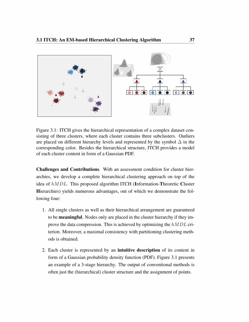
3.1 ITCH: An EM-based Hierarchical Clustering Algorithm 37
Figure 3.1: ITCH gives the hierarchical representation of a complex dataset con-sisting of three clusters, where each cluster contains three subclusters. Outliersare placed on different hierarchy levels and represented by the symbol ∆ in thecorresponding color. Besides the hierarchical structure, ITCH provides a modelof each cluster content in form of a Gaussian PDF.
Challenges and Contributions. With an assessment condition for cluster hier-archies, we develop a complete hierarchical clustering approach on top of theidea of hMDL. This proposed algorithm ITCH (Information-Theoretic ClusterHierarchies) yields numerous advantages, out of which we demonstrate the fol-lowing four:
1. All single clusters as well as their hierarchical arrangement are guaranteedto be meaningful. Nodes only are placed in the cluster hierarchy if they im-prove the data compression. This is achieved by optimizing the hMDL cri-terion. Moreover, a maximal consistency with partitioning clustering meth-ods is obtained.
2. Each cluster is represented by an intuitive description of its content inform of a Gaussian probability density function (PDF). Figure 3.1 presentsan example of a 3-stage hierarchy. The output of conventional methods isoften just the (hierarchical) cluster structure and the assignment of points.

38 3. Hierarchical Data Mining
3. ITCH has a consistent outlier-handling. Outliers are assigned to the rootof the cluster hierarchy or to an appropriate inner node, depending on thedegree of outlierness. For example, in Figures 3.1 the outlier w.r.t. thethree red clusters at the bottom level is assigned to the parent cluster in thehierarchy, marked by a red triangle.
4. ITCH is fully automatic as no difficult parameter settings are necessary.
3.1.1 Information-theoretic Hierarchical Clustering
The clustering problem is highly related to that of data compression: The detectedcluster structure can be interpreted as a PDF fΘ(x) where Θ = {θ1, θ2, ...} is aset of parameters, and the PDF can be used for an efficient compression of thedataset. It is well-known that the compression by Huffman coding is optimalif the data distribution really corresponds to fΘ(x). Huffman coding representsevery point x by a number of bits which is equal to the negative binary logarithmof the PDF:
Cdata(x) = − log2(fΘ(x)).
The better the point set corresponds to fΘ(x), the smaller the coding costsCdata(x)
are. Hence, Cdata(x) can be used as the objective function in an optimization al-gorithm. However, in data compression, Θ serves as a code book which is requiredto decode the compressed dataset again. Therefore, we need to complement thecompressed dataset with a coding of this code book, the parameter set Θ. When,for instance, a Gaussian Mixture Model (GMM) is applied, Θ corresponds to theweights, the mean vectors and the variances of the single Gaussian functions in theGMM. Considering Θ in the coding costs is also important for the clustering prob-lem, because neglecting it leads to overfitting. For partitioning (non-hierarchical)clustering structures, several approaches have been proposed for the coding ofΘ [81, 90]. These approaches differ from each other because there is no un-ambiguous and natural choice for a distribution function, which can be used for
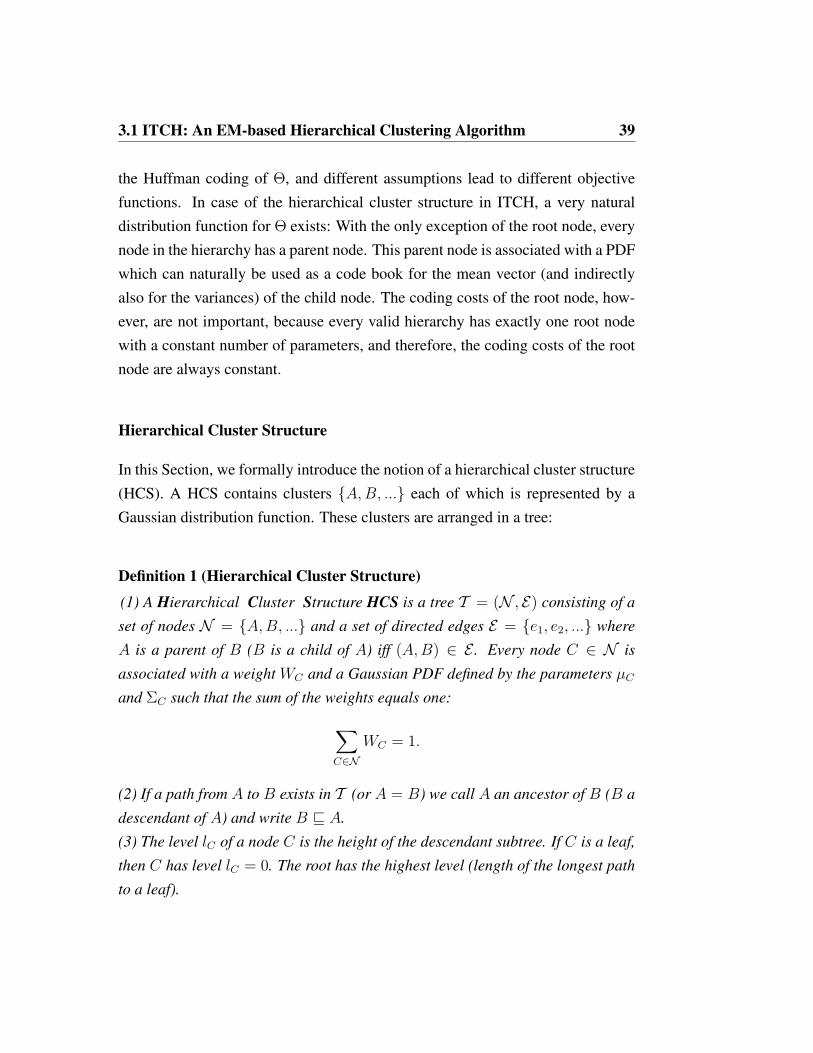
3.1 ITCH: An EM-based Hierarchical Clustering Algorithm 39
the Huffman coding of Θ, and different assumptions lead to different objectivefunctions. In case of the hierarchical cluster structure in ITCH, a very naturaldistribution function for Θ exists: With the only exception of the root node, everynode in the hierarchy has a parent node. This parent node is associated with a PDFwhich can naturally be used as a code book for the mean vector (and indirectlyalso for the variances) of the child node. The coding costs of the root node, how-ever, are not important, because every valid hierarchy has exactly one root nodewith a constant number of parameters, and therefore, the coding costs of the rootnode are always constant.
Hierarchical Cluster Structure
In this Section, we formally introduce the notion of a hierarchical cluster structure(HCS). A HCS contains clusters {A,B, ...} each of which is represented by aGaussian distribution function. These clusters are arranged in a tree:
Definition 1 (Hierarchical Cluster Structure)
(1) A Hierarchical Cluster Structure HCS is a tree T = (N , E) consisting of a
set of nodes N = {A,B, ...} and a set of directed edges E = {e1, e2, ...} where
A is a parent of B (B is a child of A) iff (A,B) ∈ E . Every node C ∈ N is
associated with a weight WC and a Gaussian PDF defined by the parameters µCand ΣC such that the sum of the weights equals one:∑
C∈N
WC = 1.
(2) If a path from A to B exists in T (or A = B) we call A an ancestor of B (B a
descendant of A) and write B v A.
(3) The level lC of a node C is the height of the descendant subtree. If C is a leaf,
then C has level lC = 0. The root has the highest level (length of the longest path
to a leaf).

40 3. Hierarchical Data Mining
The PDF which is associated with a cluster C is a multivariate Gaussian in a d-dimensional data space which is defined by the parameters µC and ΣC (whereµC = (µC,1, ..., µC,d)
T is a vector from a d-dimensional space, called the locationparameter, and ΣC is a d× d covariance matrix) by the following formula:
N(µC ,ΣC , x) =1√
(2π)d · |ΣC |· e−
12
(x−µC)T·Σ−1C ·(x−µC).
For simplicity we restrict ΣC = diag(σ2C,1, ..., σ
2C,d) to be diagonal such that the
multivariate Gaussian can also be expressed by the following product:
N(µC ,ΣC , x) =∏
1≤i≤d
N(µC,i, σ2C,i, xi)
=∏
1≤i≤d
1√2πσ2
C,i
· e− (xi−µi)
2
2σ2C,i .
Since we require the sum of all weights in a hierarchical cluster structure HCS tobe 1, a HCS always defines a function whose integral is ≤ 1. Therefore, the HCScan be interpreted as a complex, multimodal, and multivariate PDF, defined by themixture of the Gaussians of the HCS T = (N , E):
fT (x) = maxC∈N{WCN(µC ,ΣC , x)}with
∫RdfT (x)dx ≤ 1.
If the Gaussians of the HCS do not overlap much, then the integral becomes closeto 1.
The operations, described in Section 3.1.1, assign each point x ∈ DB toa cluster of the HCS T = (N , E). We distinguish between the direct and theindirect association. A point is directly associated with that cluster C ∈ N theprobability density of which is maximal at the position of x, and we write C =
Cl(x) and also x ∈ C, with:

3.1 ITCH: An EM-based Hierarchical Clustering Algorithm 41
Level 2
Level 1
Level 0
0.20.2
0.5 0.1 0.1
0.1 0.1
0.7
Figure 3.2: Hierarchical cut T ′ of the HCS T at level 1. All weights are placedinside the corresponding nodes.
Cl(x) = arg maxC∈N{WC ·N(µC ,ΣC , x)} .
As we have already stated in the introduction, one of the main motivations ofour hierarchical, information-theoretic clustering method ITCH is to represent asequence of clustering structures which range from a very coarse (unimodal) viewto the data distribution to a very detailed (multimodal) one, and that all theseviews are meaningful and represent an individual complex PDF. The ability to cuta cluster hierarchy at a given level L is obtained by the following definition:
Definition 2 (Hierarchical Cut) A HCS T ′ = (N ′, E ′) is a hierarchical cut of a
HCS T = (N , E) at level L, if the following properties hold:
(1) N ′ = {A ∈ N|lA ≥ L},(2) E ′ = {(A,B) ∈ E|lA > lB ≥ L},(3) For each A ∈ N ′ the following properties hold:
W ′A =
{WA if lA > L∑
B∈N ,BvAWB otherwise,
where WC and W ′C is the weight of node C in T and T ′, respectively.

42 3. Hierarchical Data Mining
(4) Analogously, for the direct association of points to clusters the following prop-
erty holds: Let x be associated with Cluster B in T , i.e. Cl(x) = B. Then in T ′,x is associated with:
Cl′(x) =
{B if lB ≥ L
A|B v A ∧ lA = L otherwise.
Here, the weights of the pruned nodes are automatically added to the leaf nodesof the new cluster structure, which used to be the ancestors of the pruned nodes.Therefore, the sum of all weights is maintained (and still equals 1), and the ob-tained tree is again a HCS according to Definition 1. The same holds for thepoint-to-cluster assignments. Figure 3.2 presents an illustrative example of thehierarchical cut.
Generalization of the MDL Principle
Now we explain how the MDL principle can be generalized for hierarchical clus-tering and develop the new objective function hMDL. Following the traditionalMDL principle, we compress the data points according to their negative log like-lihood corresponding to the PDF which is given by the cluster hierarchy. In ad-dition, we penalize the model complexity by adding the code length of the HCSparameters to the negative log likelihood of the data. The better the PDFs of childnodes fit into the PDFs of the parent, the less the coding costs will be. Therefore,the overall coding costs corresponds to the natural, intuitive notion of a good hier-archical representation of data by distribution functions. The discrete assignmentof points to clusters allows us to determine the coding costs of the points cluster-wise and dimensionwise, as explained in the following: The coding costs of thepoints associated with the clusters C ∈ N of the HCS T = (N , E) correspondsto:
Cdata = − log2
∏x∈DB
maxC∈N
{WC
∏1≤j≤d
N(µC,j, σ2C,j, xj)
}.

3.1 ITCH: An EM-based Hierarchical Clustering Algorithm 43
Since every point x is associated with that cluster C in the hierarchy which hasmaximum probability density, we can rearrange the terms of the above formulaand combine the costs of all points that are in the same cluster:
= −∑x∈DB
log2
(WCl(x)
∏1≤j≤d
N(µCl(x),j, σ2Cl(x),j, xj)
)= −
((∑C∈N
nWC log2WC
)+
( ∑x∈DB;
∑1≤j≤d
log2N(µCl(x),j, σ2Cl(x),j, xj)
))= −
∑C∈N
(nWC log2WC +
∑x∈C;
∑1≤j≤d
log2N(µC,j, σ2C,j, xj)
),
where WCl(x) is the weight of the cluster in the hierarchy which has maximumprobability density for the point x. The ability to model the coding costs ofeach cluster separately allows us now, to focus on a single cluster, and even ona single dimension of a single cluster. A common interpretation of the term−nWC log2WC , which actually comes from the weight a single Gaussian con-tributes to the GMM, is a Huffman coding of the cluster ID. We assume that everypoint carries the information which cluster it belongs to, and a cluster with manypoints gets a shortly coded cluster ID. These costs are referred to the ID cost of acluster C.
Consider two clusters, A and B, where B v A. We now want to derivethe coding scheme for the cluster B and its associated points. Several points areassociated with B, where the overall weight of assignment sums up to WB. Whencoding the parameters of the associated PDF of B, i.e. µB, and σB, we haveto consider two aspects: (1) The precision both parameters should be coded tominimize the overall description length depends on WB, as well as on σB. Forinstance, if only few points are associated with cluster B and/or the variance σBis very large, then it is not necessary to know the position of µB very preciselyand vice versa. (2) The knowledge of the PDF of cluster A can can be exploitedfor the coding of µB, because for likely positions (according to the PDF of A) we

44 3. Hierarchical Data Mining
mB
mB
~
(a) Exact coding of the location parameterµB . µB of the coding Gaussian function fitsexactly to µB of the data distribution.
mB
mB
~
(b) Inexact coding of the location parameterµB by some regular quantization grid.
mB
(c) Different Gaussians w.r.t. different gridpositions.
(d) Complete interval of all possible valuesfor the recovered location parameter µB w.r.t.to the PDF of the predecessor cluster A.
Figure 3.3: Optimization of coding scheme for the location parameter.

3.1 ITCH: An EM-based Hierarchical Clustering Algorithm 45
can assign fewer bits. Basically, model selection criteria, such as the BayesianInformation Criterion (BIC) or the Aikake Information Criterion (AIC) alreadyaddress the first aspect, but not the hierarchical aspect. To make this thesis selfcontained, we consider both aspects. In contrast to BIC, which uses the naturallogarithm, we use the binary logarithm to represent the code length in bits. Forsimplicity, we assume that our PDF is univariate and the only parameter is its meanvalue µB. We neglect σB by assuming e.g. some fixed value for all clusters. Wedrop these assumptions at the end of this section. When the true PDF of cluster Bis coded inexactly by some parameter µB, the coding costs for each point x (whichtruly belongs to the distribution N(µB, σ
2B, x)) in B is increased compared to the
exact coding of µB, which would result in cex bits per point:
cex =
∫ +∞
−∞− log2(N(µB, σ
2B, x)) ·N(µB, σ
2B, x) dx = log2(σB
√2π · e).
If µB instead of µB is applied for compression, we obtain:
c(µB, µB) =
∫ +∞
−∞− log2(N(µB, σ
2B, x)) ·N(µB, σ
2B, x)dx.
The difference is visualized in Figure 3.3(a) and 3.3(b) respectively: In 3.3(a) µBof the coding PDF, depicted by the Gaussian function, fits exactly to µB of the datadistribution, represented by the histogram. This causes minimum code lengths forthe compressed points but also a considerable effort for the coding of µB. InFigure 3.3(b) µB is coded by some regular quantization grid. Thereby, the costsfor the cluster points slightly increase, but the costs for the location parameterdecreases. The difference between µB and µB depends on the bit resolution and onthe position of the quantization grid. One example is depicted in Figure 3.3(b) byfive vertical lines, the Gaussian curve is centered by the vertical line closest to µB.We derive lower and upper limits of µB ∈ [µB−1/2b...µB+1/2b] from the numberof bits b, spent for coding µB. The real difference between µB and µB dependsagain on the grid position. Not to prefer clusters that are incidentally aligned with

46 3. Hierarchical Data Mining
the grid cells, we average over all possible positions of the discretization grid.Figure 3.3(c) presents five different examples of the infinitely many Gaussiansthat could be recovered w.r.t. different grid positions. Note that all positionsinside the given interval have equal probability. Hence, the average coding costsfor every possible position of µB can be expressed by the following integral:
cappx(b) = 2b−1
∫ µB+1/2b
µB−1/2bc(µB, µB) dµB
=1
2log2(π · e · σ2
B) +1
2+
log2 e6 · σ2
B
· 4−b.
Coding all n ·WB coordinates of the cluster points as well as the parameter µB(neglecting the ID cost) requires then the following number of bits:
Cappx(B) = cappx(b) · n ·WB + b.
The optimal number bopt of bits is determined by setting the derivation of theabove term to zero.
ddbCappx(B) = 1− 4−b · n ·WB
3 · σ2B
= 0 =⇒ bopt =1
2log2(
n ·WB
3 · σ2B
).
The unique solution to this equation corresponds to a minimum, as inserting boptinto the second derivative
d2
db2Cappx(B) =
4−b · n ·WB · log2(4)
3 · σ2B
leads to a positive value.

3.1 ITCH: An EM-based Hierarchical Clustering Algorithm 47
Utilization of the Hierarchical Relationship. We do not want to code the (inex-act) position of µB without the prior knowledge of the PDF associated with clusterA. Without this knowledge, we would have to select a suitable range of values andcode µB at the determined precision b assuming e.g. a uniform distribution insidethis range. In contrast, µB is a value taken from the distribution function of clus-ter A. Hence, the number of bits used for coding of µB corresponds to the overalldensity around the imprecise interval defined by µB, i.e.
chMDL(µB) = − log2
∫ µB+1/2b
µB−1/2bN(µA, σ
2A, x) dx.
Figure 3.3(d) visualizes the complete interval of all possible values for the recov-ered mean value (marked in red) and illustrates the PDF of the clusterA, whichis the predecessor of cluster B. µB can be coded by determining the whole areaunder the PDF of A where µB could be. The area actually corresponds to a prob-ability value. The negative logarithm of this probability represents the requiredcode length for µB. The costs for coding all points of cluster B and µB thencorresponds to
cappx(b) · n ·WB + chMDL(µB).
Note, that it is also possible to optimize b directly by setting the derivative of thisformula to zero. However, this is impossible in an analytic way, and the differenceto the optimum which is obtained by minimizing Cappx(B) is negligible. Inaddition, if the parent A of B is not the root of the hierarchy, µB causes some ownID cost. In this case, µB is a sample from the complex distribution function ofthe hierarchical cut (cf. Definition 2), which prunes the complete level of B andall levels below. Hence, the weight of these levels is added to the new leaf nodes(after cutting), and the ID costs of µB correspond to:
− log2 (∑XvA
WX).

48 3. Hierarchical Data Mining
A similar analysis can be done for the second parameter of the distribution func-tion, σB. Since it is not straightforward to select a suitable distribution function forthe Huffman coding of variances, one can apply a simple trick: Instead of codingσB, we code yB = µB±v ·σB, where v is a constant close to zero. Then, yB is alsoa sample from the distribution function N(µA, σ
2A, x) and can be coded similar to
µB. Therefore, chMDL(σB) = chMDL(µB), and we write chMDL(param) forthe coding costs per parameter instead. In general, if the PDF, which is associatedwith a cluster has r parameters, then the optimal number of bits can be obtainedby the formula:
bopt =1
2log2(
n ·WB
3 · r · σ2B
).
And the overall coding costs are:
ChMDL(B) = cappx(b) · n ·WB + r · chMDL(param)
Until now, only the tradeoff between coding costs of points and the parametersof the assigned cluster are taken into account. If we go above the lowest levelof the cluster hierarchy, we have to trade between coding costs of parameters ata lower level and coding costs of the parameters at the next higher level. Thiscan be done in a similar way as before: Let bB be the precision, which has alreadybeen determined for the representation of µB and σB, the parameters for clusterB,which is a subcluster of A. However, this is the minimum coding costs assumingthat µA and σA have been stored at maximum precision, and that µB and σB
are also given. Now, we assume that µB is an arbitrary point selected from thedistribution function N(µA, σ
2A, x) and determine an expectation for the cost:
∫ +∞
−∞− log2
∫ µB+1/2bB
µB−1/2bBN(µA, σ
2A, x)dx N(µA, σ
2A, µB)dµB.
Finally, we assume that µA is also coded inexactly by its own grid with resolutionbA. Then the expected costs are:
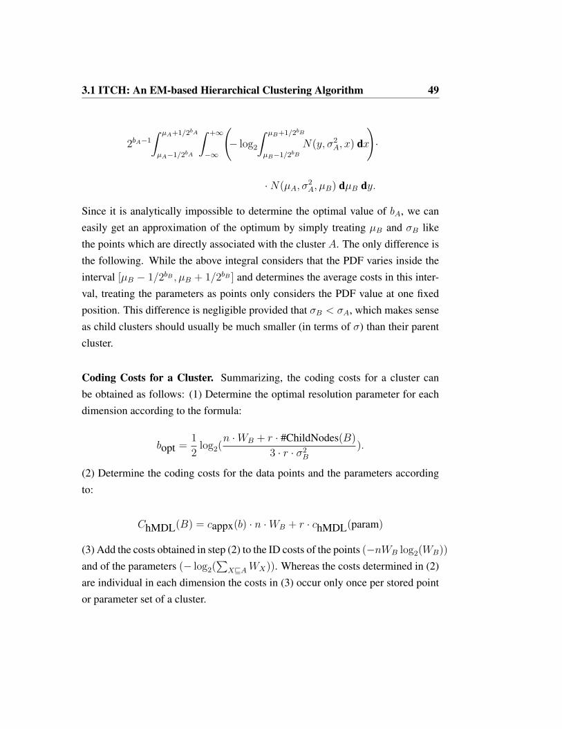
3.1 ITCH: An EM-based Hierarchical Clustering Algorithm 49
2bA−1
∫ µA+1/2bA
µA−1/2bA
∫ +∞
−∞
(− log2
∫ µB+1/2bB
µB−1/2bBN(y, σ2
A, x) dx
)·
·N(µA, σ2A, µB) dµB dy.
Since it is analytically impossible to determine the optimal value of bA, we caneasily get an approximation of the optimum by simply treating µB and σB likethe points which are directly associated with the cluster A. The only difference isthe following. While the above integral considers that the PDF varies inside theinterval [µB − 1/2bB , µB + 1/2bB ] and determines the average costs in this inter-val, treating the parameters as points only considers the PDF value at one fixedposition. This difference is negligible provided that σB < σA, which makes senseas child clusters should usually be much smaller (in terms of σ) than their parentcluster.
Coding Costs for a Cluster. Summarizing, the coding costs for a cluster canbe obtained as follows: (1) Determine the optimal resolution parameter for eachdimension according to the formula:
bopt =1
2log2(
n ·WB + r · #ChildNodes(B)
3 · r · σ2B
).
(2) Determine the coding costs for the data points and the parameters accordingto:
ChMDL(B) = cappx(b) · n ·WB + r · chMDL(param)
(3) Add the costs obtained in step (2) to the ID costs of the points (−nWB log2(WB))
and of the parameters (− log2(∑
XvAWX)). Whereas the costs determined in (2)are individual in each dimension the costs in (3) occur only once per stored pointor parameter set of a cluster.

50 3. Hierarchical Data Mining
Coding Costs for the HCS. The coding costs for all clusters sum up to the overallcoding costs of the hierarchy where we define constant ID costs for the parametersof the root:
hMDL =∑C∈N
(ChMDL(C)− nWC log2(WC)− log2(
∑Xvparent of C
WX)
)·
Obtaining and Optimizing the HCS
We optimize our objective function in an EM-like clustering algorithm ITCH. Re-assignment of objects and re-estimation of the parameters of the cluster hierarchyare done interchangeably until convergence. Starting from a suitable initialization,ITCH periodically modifies the hierarchy.
Initialization of the HCS. Clustering algorithms that follow the EM-scheme haveto be suitable initialized before starting with the actual iterations of E- and M-step.An established method is to initialize with the result of a k-means [72] clustering.This is typically repeated several times with different seeds and the result withbest mean squared overall deviation from the cluster centers is taken. Followingthis idea, ITCH uses an initialization hierarchy determined by a bisecting k-meansalgorithm taking the hMDL value of the HCS as a stopping criterion for parti-tioning. First, a root node that contains all points is created. Then this root nodeis partitioned into two subclusters by applying k-means with k = 2. This is donerecursively until the hMDL of the binary hierarchy does not improve anymorewithin three steps. This ensures not to get stuck in a local minimum. Finally,after the best hierarchy is selected, µC and ΣC are determined for each node Caccording to Section 3.1.1, and equal weights are assigned to the nodes, to ensurethat clusters compete likewise for the data points.
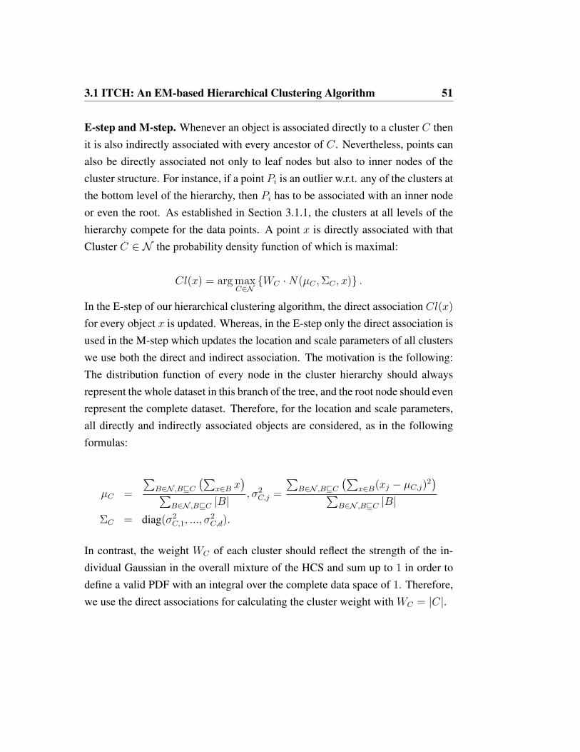
3.1 ITCH: An EM-based Hierarchical Clustering Algorithm 51
E-step and M-step. Whenever an object is associated directly to a cluster C thenit is also indirectly associated with every ancestor of C. Nevertheless, points canalso be directly associated not only to leaf nodes but also to inner nodes of thecluster structure. For instance, if a point Pi is an outlier w.r.t. any of the clusters atthe bottom level of the hierarchy, then Pi has to be associated with an inner nodeor even the root. As established in Section 3.1.1, the clusters at all levels of thehierarchy compete for the data points. A point x is directly associated with thatCluster C ∈ N the probability density function of which is maximal:
Cl(x) = arg maxC∈N{WC ·N(µC ,ΣC , x)} .
In the E-step of our hierarchical clustering algorithm, the direct association Cl(x)
for every object x is updated. Whereas, in the E-step only the direct association isused in the M-step which updates the location and scale parameters of all clusterswe use both the direct and indirect association. The motivation is the following:The distribution function of every node in the cluster hierarchy should alwaysrepresent the whole dataset in this branch of the tree, and the root node should evenrepresent the complete dataset. Therefore, for the location and scale parameters,all directly and indirectly associated objects are considered, as in the followingformulas:
µC =
∑B∈N ,BvC
(∑x∈B x
)∑B∈N ,BvC |B|
, σ2C,j =
∑B∈N ,BvC
(∑x∈B(xj − µC,j)2
)∑B∈N ,BvC |B|
ΣC = diag(σ2C,1, ..., σ
2C,d).
In contrast, the weight WC of each cluster should reflect the strength of the in-dividual Gaussian in the overall mixture of the HCS and sum up to 1 in order todefine a valid PDF with an integral over the complete data space of 1. Therefore,we use the direct associations for calculating the cluster weight with WC = |C|.

52 3. Hierarchical Data Mining
C
(a) Detail of the initial state ofa given hierarchy.
(b) Hierarchy afterdeleting cluster C.
C´
(c) Hierarchy aftercollapsing cluster Cwith its child nodes.
Figure 3.4: Restructure operations of ITCH.
Rearrangement of the HCS. The binary hierarchy that results from the initializa-tion, does not limit our generality. ITCH is flexible enough to convert the initialcluster structure into a general one. Given a binary hierarchy, which is deeperthan any n-ary hierarchy with n > 2, ITCH aims in flattening the hierarchy as faras the rearrangement improves the hMDL criterion. Therefore we trade off thetwo operations delete or collapse a node to eliminate clusters that do not pay offany more. Figure 3.4 visualizes the operations for an extract of a given HCS. Bydeleting a cluster C, the child nodes of C become child nodes of the parent of C(cf. Figure 3.4(b)). By collapsing C, all of its child nodes are merged into a newcluster C ′ (including C), and therefore all of their child nodes become child nodesof C ′ (cf. Figure 3.4(c)). Afterwards all points are redistributed, and E- and M-step are performed alternately until convergence. ITCH rearranges the structurein an iterative way. In each iteration we tentatively delete/collapse each node inthe hierarchy and perform E- and M-steps. Then first, the node and the operationthat improves the hMDL criterion best is selected and second, the correspondinglocal neighborhood (parent, child and sibling nodes) is processed.

3.1 ITCH: An EM-based Hierarchical Clustering Algorithm 53
3.1.2 Experimental Evaluation
Since ITCH is a hybrid approach combining the benefits of hierarchical and model-based clustering, we compare to algorithms of both classes to demonstrate theeffectiveness of ITCH. We selected Single Link (SL) [53] which probably is themost common approach to hierarchical clustering. As especially on noisy data,SL suffers from the so-called Single Link effect, we additionally compare to OP-TICS [4], a more outlier-robust hierarchical clustering algorithm, with a standardparameterization of MinPts = 6 and epsilon = 0.9. Furthermore, we com-pare to RIC [10], an outlier-robust and parameter-free state-of-the-art algorithmto model-based clustering. ITCH is implemented in Java. SL was provided byMatlab and OPTICS was provided by WEKA [42]. For RIC we used the originalimplementations by the authors.
For each dataset, the clustering results were assessed against a ground-truthclassification. To compare the clustering results produced by different approaches,we chose measures that comprise fix bounds. More precisely, we selected thefollowing recently proposed information-theoretic methods [77]: the Normal-ized Mutual Information (NMI), the Adjusted Mutual Information (AMI), andthe Expected Mutual Information (EMI). These three information-theoretic mea-sures are based on the general mutual information (MI) of two given clusteringsC = {C1, · · · , Cl} and C ′ = {C1, · · · , Ck} of a dataset DS and a contingencytable M = [mij]
i=1,··· ,lj=1,··· ,k, where each entry denotes the number of common ob-
jects of both clusterings. Hence, MI is a symmetric measure that quantifies theinformation that the two clusterings C and C ′ share. Formally it is defined asfollows:
MI(C,C ′) =l∑
i=1
k∑j=1
p(i, j) logp(i, j)
p(i)p(j),
where p(i, j) denotes the probability that a point belongs to cluster Ci ∈ C andcluster C ′j ∈ C ′. The NMI then is a normalized version of the MI, by a divisionby the maximum value of the index. It takes a value of 1 if two clusterings are

54 3. Hierarchical Data Mining
identical and 0 if the two clusterings are independent. The AMI is based on theEMI, and is corrected for randomness. It takes a value of 1 if the two clusteringsare identical and 0 if the mutual information between the two clusterings equalsits expected value. The EMI defines the average mutual information between allpairs of clusterings that have the same number of clusters and objects in eachcluster as in the two given clusters C and C ′. Also the EMI take the value of 1 ifthe resulting clustering corresponds exactly to the ground-truth classification, and0 if both clusterings are totally independent.
Furthermore, we chose the well-known Precision (Prec) and Recall (Rec) frominformation retrieval. The Precision of a cluster can be seen as a measure ofexactness and is defined as the fraction of the clustered datapoints that are labeledby the true class label (named true positives) devided by all data points of thespecific cluster. The Recall is a measure of completeness. It is defined as theproportion of the true positives against all data points that are labeled by the classlabel of the specific cluster.
Finally, we use the measure proposed by DOM et al. [30], referred to as DOMin the following, that corresponds to the number of bits required to encode theclass labels when the cluster labels are known. If the number of clusters is equalin both clusterings C and C ′, DOM is equal to the mutual information. In cases,where the number of clusters is different, it computes the reduction in number ofbits that would be required to encode the class labels. Hence, small DOM valuesrefer to good clusterings.
Synthetic Data
Experiments onDS1 demonstrate the superiority of ITCH on hierarchical datasets.DS1 comprises about 3,500 2-dimensional points that form a hierarchy of 12 clus-ters with outliers at different levels of the hierarchy. Seven Gaussian clusters arelocated at the bottom level (cf. Figure 3.5(a)). Experiments on DS2 indicatethe limitations of existing approaches to form meaningful clusters in extremelynoisy non-hierarchical data. DS2 is composed of two Gaussian clusters with

3.1 ITCH: An EM-based Hierarchical Clustering Algorithm 55
1,650 points each, overlapping in the marginal area without any global outliers(cf. Figure 3.5(b)).
2 clusters with local noise
2 local outliers
2 clusters with local noise
3 clusters with local noise
(a) Plotted DS1. (b) Plotted DS2.
Figure 3.5: The synthetic datasetDS1 forms a hierarchy including local noise withdifferent degrees of outlierness. DS2 consists of two highly overlapping clusters.It comprises no outliers.
Experimental Evaluation on DS1. As clusters can be recognized as valleys inthe reachability plot illustrated in Figure 3.6(a), OPTICS yields a satisfactory so-lution resulting in good validity values (cf. Table 3.1) w.r.t. a cut through thehierarchy at a maximum reachability distance of 0.02. But one has to notice thatit is hard to spot the outliers since high distance peaks can also be caused by theusual jumps. Also, the SL-hierarchy (cf. Figure 3.6(b)) represents the true hierar-chy quite well. The reason for that is that DS1 comprises a hierarchy that can berecognized by agglomerative clustering algorithms relatively easy. However, theDOM value of 0.2142 reflects that the clustering information of the outlier objectscauses slightly more coding costs, as the red cluster on the right side suffers froma slight Single Link effect. All values shown in Table 3.1 refer to a cut throughthe dendrogram at a cutoff value of 10, resulting in seven disjoint clusters.
In order to apply RIC to the hierarchical dataset, we preprocessed DS1 with SLand applied RIC (k = 18) as postprocessing step in each level of the hierarchy.

56 3. Hierarchical Data Mining
Cut w.r.t. reachability distance = 0.02
2 clusters with local
noise
2 clusters with local
noise
3 clusters with local noise
(a) OPTICS on DS1.
Cutoff value = 10
(b) SL on DS1.
2 + 2 clusters with local noise
3 clusters with local noise
local noise
Root cluster
(c) The result of ITCH on DS1 comprises the hierarchical cluster structure and the PDF of eachcluster content.
Figure 3.6: Competitive evaluation of ITCH on the synthetic dataset DS1.
Table 3.1 shows the validation of the corresponding clustering result. Even RICfails to successfully filter out all outliers. More precisely, it assigns points that ob-viously are local outliers misleadingly to clusters. Also a majority of the outliersare incorrectly identified as cluster points. Hence, RIC performs worst on the hier-archical dataset DS1 concerning the quantitative analysis presented in Table 3.1.Only ITCH detects the true cluster hierarchy including outliers fully automati-cally, and provides meaningful models on the data for each level of the hierarchy(cf. Figure 3.6(c)).
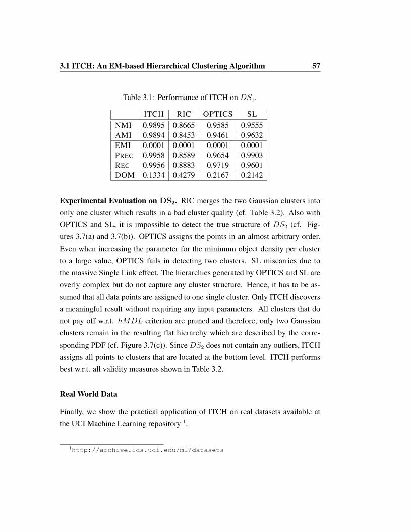
3.1 ITCH: An EM-based Hierarchical Clustering Algorithm 57
Table 3.1: Performance of ITCH on DS1.
ITCH RIC OPTICS SLNMI 0.9895 0.8665 0.9585 0.9555AMI 0.9894 0.8453 0.9461 0.9632EMI 0.0001 0.0001 0.0001 0.0001PREC 0.9958 0.8589 0.9654 0.9903REC 0.9956 0.8883 0.9719 0.9601DOM 0.1334 0.4279 0.2167 0.2142
Experimental Evaluation on DS2. RIC merges the two Gaussian clusters intoonly one cluster which results in a bad cluster quality (cf. Table 3.2). Also withOPTICS and SL, it is impossible to detect the true structure of DS2 (cf. Fig-ures 3.7(a) and 3.7(b)). OPTICS assigns the points in an almost arbitrary order.Even when increasing the parameter for the minimum object density per clusterto a large value, OPTICS fails in detecting two clusters. SL miscarries due tothe massive Single Link effect. The hierarchies generated by OPTICS and SL areoverly complex but do not capture any cluster structure. Hence, it has to be as-sumed that all data points are assigned to one single cluster. Only ITCH discoversa meaningful result without requiring any input parameters. All clusters that donot pay off w.r.t. hMDL criterion are pruned and therefore, only two Gaussianclusters remain in the resulting flat hierarchy which are described by the corre-sponding PDF (cf. Figure 3.7(c)). Since DS2 does not contain any outliers, ITCHassigns all points to clusters that are located at the bottom level. ITCH performsbest w.r.t. all validity measures shown in Table 3.2.
Real World Data
Finally, we show the practical application of ITCH on real datasets available atthe UCI Machine Learning repository 1.
1http://archive.ics.uci.edu/ml/datasets
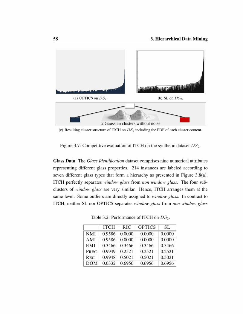
58 3. Hierarchical Data Mining
(a) OPTICS on DS2. (b) SL on DS2.
2 Gaussian clusters without noise
(c) Resulting cluster structure of ITCH on DS2 including the PDF of each cluster content.
Figure 3.7: Competitive evaluation of ITCH on the synthetic dataset DS2.
Glass Data. The Glass Identification dataset comprises nine numerical attributesrepresenting different glass properties. 214 instances are labeled according toseven different glass types that form a hierarchy as presented in Figure 3.8(a).ITCH perfectly separates window glass from non window glass. The four sub-clusters of window glass are very similar. Hence, ITCH arranges them at thesame level. Some outliers are directly assigned to window glass. In contrast toITCH, neither SL nor OPTICS separates window glass from non window glass
Table 3.2: Performance of ITCH on DS2.
ITCH RIC OPTICS SLNMI 0.9586 0.0000 0.0000 0.0000AMI 0.9586 0.0000 0.0000 0.0000EMI 0.3466 0.3466 0.3466 0.3466PREC 0.9949 0.2521 0.2521 0.2521REC 0.9948 0.5021 0.5021 0.5021DOM 0.0332 0.6956 0.6956 0.6956
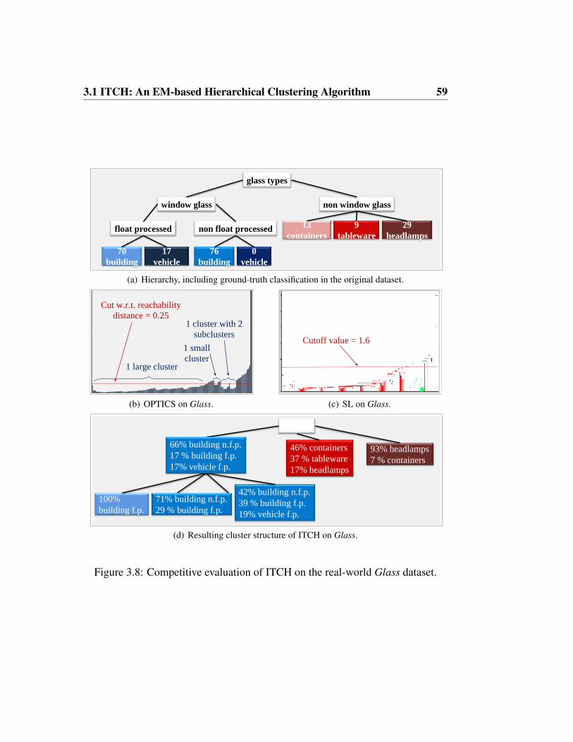
3.1 ITCH: An EM-based Hierarchical Clustering Algorithm 59
29
headlamps
9
tableware
13
containers
0
vehicle
76
building
17
vehicle
70
building
float processed non float processed
window glass non window glass
glass types
(a) Hierarchy, including ground-truth classification in the original dataset.
Cut w.r.t. reachability distance = 0.25
1 cluster with 2 subclusters
1 large cluster
1 small cluster
subclusters
(b) OPTICS on Glass.
Cutoff value = 1.6
(c) SL on Glass.
93% headlamps
7 % containers
46% containers
37 % tableware
17% headlamps
42% building n.f.p.
39 % building f.p.
19% vehicle f.p.
100%
building f.p.
71% building n.f.p.
29 % building f.p.
66% building n.f.p.
17 % building f.p.
17% vehicle f.p.
(d) Resulting cluster structure of ITCH on Glass.
Figure 3.8: Competitive evaluation of ITCH on the real-world Glass dataset.

60 3. Hierarchical Data Mining
perfectly. In the dendrogram one large cluster and one medium size cluster is vis-ible, whereas OPTICS determines two clusters of different size and one clusterwith two nested subclusters. RIC, applied at the bottom level of the SL resultcomprises only two clusters without any separation between window glass or non
window glass. Table 3.3 summarizes the quantitative analysis of this dataset. ForOPTICS the results refer to the partitioning clustering with a maximum reachabil-ity distance of 0.25. The SL results indicate the results for a cutoff value of 1.6.
Table 3.3: Performance of ITCH on the real-world Glass dataset.
ITCH RIC OPTICS SLNMI 0.3390 0.1221 0.4029 0.4110AMI 0.3222 0.0804 0.3092 0.3085EMI 0.0018 0.0010 0.0017 0.0012PREC 0.5350 0.1710 0.4739 0.3812REC 0.3551 0.1822 0.4626 0.4393DOM 1.4805 1.5872 1.2980 1.5010
Cancer Data. The high-dimensional Breast Cancer Wisconsin dataset contains569 instances each describing 30 different characteristics of the cell nuclei, whereeach instance is either labeled by benign (blue) or malignant (red). OPTICS andSL both fail to detect a clear cluster structure in this dataset. OPTICS finds onelarge cluster and one very small cluster that could also be interpreted as noise(cf. Figures 3.9(a)). In the dendrogram of SL, shown in Figure 3.9(b), one largeand many small clusters are visible. The quantitative evaluation represented inTable 3.4 refer to a cutoff value of 60.We applied RIC on top of a k-means clustering with k = 15. As stated by the au-thors we chose k large enough compared to the number of classes. However, RICalso fails and results in three mixed clusters. ITCH almost perfectly separates thebenign from the malignant objects which are then split into different subclusters(cf. Figure 3.9(c)). This precise structure is penalized by the validity measuressummarized in Table 3.4. However, this result is consistent with previous findings
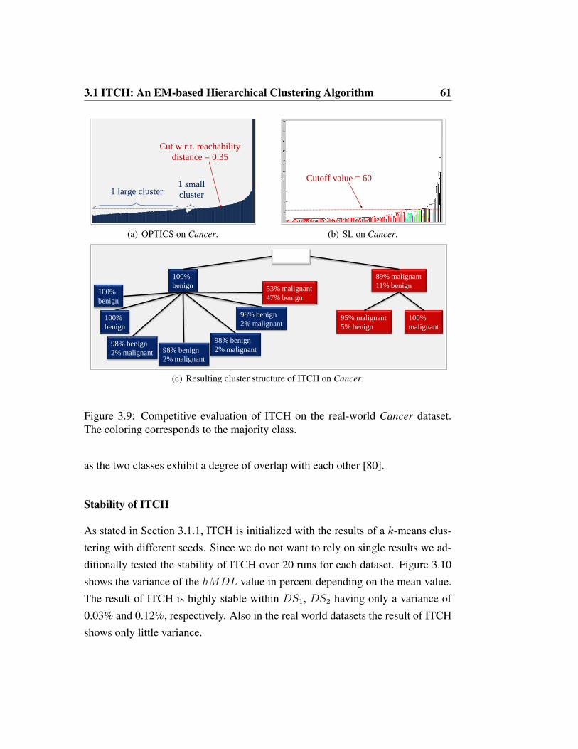
3.1 ITCH: An EM-based Hierarchical Clustering Algorithm 61
Cut w.r.t. reachability distance = 0.35
1 small cluster1 large cluster
(a) OPTICS on Cancer.
Cutoff value = 60
(b) SL on Cancer.
100%
malignant
53% malignant
47% benign
95% malignant
5% benign
100%
benign
100%
benign
98% benign
2% malignant 98% benign
2% malignant
98% benign
2% malignant
98% benign
2% malignant
100%
benign
89% malignant
11% benign
(c) Resulting cluster structure of ITCH on Cancer.
Figure 3.9: Competitive evaluation of ITCH on the real-world Cancer dataset.The coloring corresponds to the majority class.
as the two classes exhibit a degree of overlap with each other [80].
Stability of ITCH
As stated in Section 3.1.1, ITCH is initialized with the results of a k-means clus-tering with different seeds. Since we do not want to rely on single results we ad-ditionally tested the stability of ITCH over 20 runs for each dataset. Figure 3.10shows the variance of the hMDL value in percent depending on the mean value.The result of ITCH is highly stable within DS1, DS2 having only a variance of0.03% and 0.12%, respectively. Also in the real world datasets the result of ITCHshows only little variance.

62 3. Hierarchical Data Mining
Table 3.4: Performance of ITCH on the real-world Cancer dataset.
ITCH RIC OPTICS SLNMI 0.3821 0.4594 0.2835 0.3097AMI 0.2044 0.3612 0.2518 0.2127EMI 0.0004 0.0003 0.0003 0.0006PREC 0.9574 0.9846 0.8033 0.8884REC 0.2830 0.6608 0.7575 0.6626DOM 0.2635 0.3022 0.4752 0.4771
45150
45160
DL
valu
e
45120
45130
45140
mea
n hM
D
(a) DS1
32010
32030
32050
DL
valu
e
31950
31970
31990
32010
mea
n hM
D
(b) DS2
-3500
-3400
-3300
DL
valu
e-3800
-3700
-3600
3500
mea
n hM
D
(c) Glass
-10700
-10500
-10300
DL
valu
e
-11300
-11100
-10900
10700
mea
n hM
D
(d) Cancer
Figure 3.10: Stability of the ITCH results, determined over 20 runs for eachdataset.
3.1.3 Conclusions
We have introduced a new hierarchical clustering method to arrange only natu-ral, valid, and meaningful clusters in a hierarchical structure – ITCH. ITCH isbased on an objective function for clustering that was guided by the information-theoretic idea of data compression. We have shown that without difficult param-eter settings ITCH finds the real cluster hierarchy effectively, and that it providesaccurate and intuitive interpretable information in a wide variety of domains, evenin the presence of local and global outliers that correspond to inner nodes of theresulting hierarchy.

3.2 GACH: A Genetic Algorithm for Hierarchical Clustering 63
3.2 GACH: A Genetic Algorithm for HierarchicalClustering
Many EM-based algorithms, including ITCH, suffer from the problem that theyoften get stuck in a local optimum. One solution that overcomes that problem isthe application of genetic algorithms (GAs). A GA is a stochastic optimizationtechnique based on the mechanism of natural selection and genetics, originallyproposed by [45]. The general idea behind a GA is that the candidate solutions toan optimization problem (called individuals) are often encoded as binary strings(called chromosomes). A collection of these chromosomes forms a population.The evolution initially starts from a random population that represents differentindividuals in the search space. In each generation, the fitness of every individualis evaluated, and multiple individuals are then selected from the current populationbased on Darwin’s principle “Surviving of the fittest”. These individuals buildthe mating pool for the next generation. The new population is then formed bythe application of recombination operations like crossover and mutation. A GAcommonly terminates when either a maximum number of generations has beenproduced, or a satisfactory fitness level has been reached for the population. Asurvey of GAs along with the programming structure used can be found in [34].
GAs have been successfully applied to a variety of challenging optimiza-tion problems, like image processing, neural networks and machine learning,etc. [79, 104, 6]. Solving the NP-hard clustering problem makes GA thereforea natural choice such as in [60, 26, 74, 86, 70, 82]. Our motivation for usingGAs for hierarchical clustering is visualized in Figure 3.11. The clustering re-search community focuses on clustering methods where the grouped objects aredescribed by an intuitive model of the data [28] or clustering methods that areparticularly insensitive to outliers [31]. Moreover, several approaches have alsobeen addressing the question, how to avoid difficult parameter settings such as thenumber of clusters, e.g. [81, 43, 10, 11, 12]. Most of them meet this question byrelating the clustering problem with the idea of data compression.

64 3. Hierarchical Data Mining
Global
outlier
Intuitive description for each cluster
GACHSearch space
Figure 3.11: The search space of the solutions for the hierarchical clustering prob-lem is exponentially large. Genetic algorithms help to determine the global op-timum. GACH is a genetic algorithm for finding the most meaningful clusterhierarchy. Outliers are assigned to appropriate inner nodes. Each cluster contentis described by an intuitive description in form of a PDF.
Here we present a novel genetic algorithm for finding cluster hierarchies, calledGACH. We use an information-theoretic fitness function to effectively cluster datainto meaningful hierarchical structures without requiring the number of clustersas an input parameter. Our major contributions are:
• Fitness: The fitness of different chromosomes is optimized using the sameMDL-based optimization technique as used for ITCH.
• No difficult parameter-setting: Besides the parameters that are specific fora genetic algorithm, GACH requires no expertise about the data (e.g. thenumber of clusters).
• Flexibility: By the use of a GA-based stochastic search GACH thoroughlyexplores the search space and is therefore flexible enough to find the correcthierarchical cluster structure and is not sensitive to the initialization.
• Outlier-handling: Outliers are assigned to the root of the cluster hierarchyor to an appropriate inner node, depending on the degree of outlierness.
• Model description: The content of each cluster is described by a PDF.
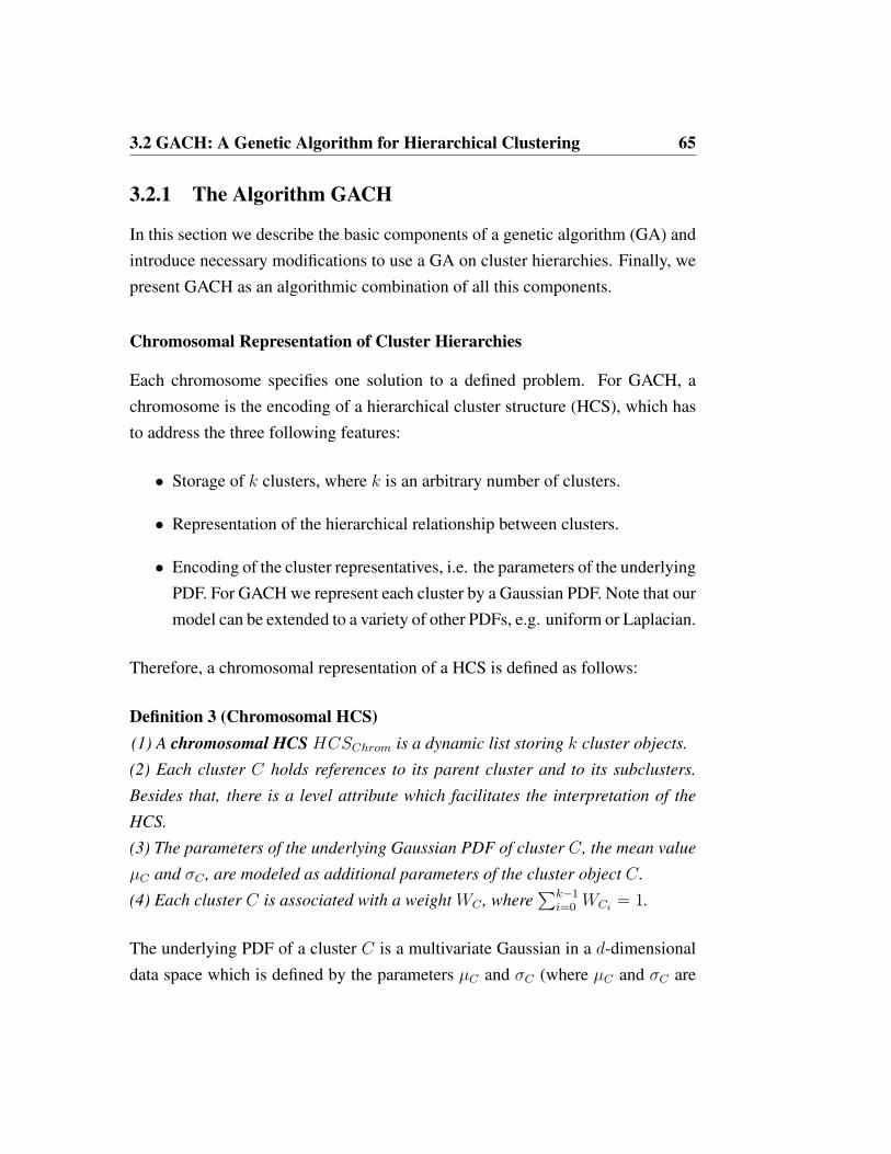
3.2 GACH: A Genetic Algorithm for Hierarchical Clustering 65
3.2.1 The Algorithm GACH
In this section we describe the basic components of a genetic algorithm (GA) andintroduce necessary modifications to use a GA on cluster hierarchies. Finally, wepresent GACH as an algorithmic combination of all this components.
Chromosomal Representation of Cluster Hierarchies
Each chromosome specifies one solution to a defined problem. For GACH, achromosome is the encoding of a hierarchical cluster structure (HCS), which hasto address the three following features:
• Storage of k clusters, where k is an arbitrary number of clusters.
• Representation of the hierarchical relationship between clusters.
• Encoding of the cluster representatives, i.e. the parameters of the underlyingPDF. For GACH we represent each cluster by a Gaussian PDF. Note that ourmodel can be extended to a variety of other PDFs, e.g. uniform or Laplacian.
Therefore, a chromosomal representation of a HCS is defined as follows:
Definition 3 (Chromosomal HCS)(1) A chromosomal HCS HCSChrom is a dynamic list storing k cluster objects.
(2) Each cluster C holds references to its parent cluster and to its subclusters.
Besides that, there is a level attribute which facilitates the interpretation of the
HCS.
(3) The parameters of the underlying Gaussian PDF of cluster C, the mean value
µC and σC , are modeled as additional parameters of the cluster object C.
(4) Each cluster C is associated with a weight WC , where∑k−1
i=0 WCi = 1.
The underlying PDF of a cluster C is a multivariate Gaussian in a d-dimensionaldata space which is defined by the parameters µC and σC (where µC and σC are

66 3. Hierarchical Data Mining
vectors from a d-dimensional space) by the following formula:
N(µC , σC , x) =∏
1≤i≤d
1√2πσ2
C,i
· e−
(xi−µC,i)2
2σ2C,i
GACH assigns each point x ∈ DB directly to that cluster C ∈ HCSChrom theprobability density of which is maximal at the position of x:
C(x) = arg maxC∈HCSChrom
{WC ·N(µC , σC , x)} .
Initialization of GACH
In a GA, the initial set of a population consists of a randomly generated set ofindividuals. Therefore, GACH selects a random number of clusters k for eachstructure HCSChrom in a first step. Then a simple k-means algorithm [72] dividesthe dataset into k clusters representing the leafs of the initial hierarchy. Finally,these clusters are combined by one additional root cluster. Hence, the initializationprocess results in a 2-level hierarchy that consists of k + 1 nodes. Each cluster Cis described by random parameters and is associated to a weight WC = 1
k.
Reproduction
In order to generate the next population, GACH uses several genetic operators thatare particularly defined for the hierarchical clustering problem. As our algorithmis initialized by a flat hierarchy generated by a partitioning clustering procedure,GACH needs mutating oparators that add nodes to the hierachy. However, onlyadding new nodes would not leed to sufficient results because parameters like µ,σ and the cluster weight are chosen randomly. Therefore, we need a further op-erator which demotes given nodes to different hierarchy levels. Additionally, thecentral goal of a genetic algorithm is an efficient eradication of the search space.Hence, we need for each mutation operator also the inverse procedure to avoid to

3.2 GACH: A Genetic Algorithm for Hierarchical Clustering 67
get stuck in only a local optimum. Finally, we use the mutations add, delete,demote and promote, and the GA-specific operator crossover.
The operator add adds direct subclusters to an arbitrary cluster C of the hierarchywith an add rate padd (normally pdel = padd). The number of added subclusters isbounded by an upper limit valuemaxnew. Figure 3.12(a) illustrates an example forthe application of the add operator to a HCS. One subcluster (marked in dark bluecolor) is added to the red cluster. Since the cluster content of a added subclusterCadd is covered by the cluster content ofC, we calculate random parameters basedon µC and σC . In particular, we add a random factor r to both parameters, wherer is a vector from a d-dimensional space: µCadd = µC + r σCadd = σC + r.
The operator delete deletes a specific cluster C (except the root) with a dele-tion rate pdel from the HCS. This results in structure HCS′ that does not containthe cluster C anymore. (cf. Figure 3.12(b)). Here, the cluster C is marked by darkblue color. The level of each direct and indirect subcluster of C (marked in red)is decreased by 1. The former parent node of C, the root node in our example,becomes the parent node of all direct subclusters of C.
The motivation behind the demote operator is the following. Assume a datasetconsisting of three clusters C1, C2 and C3, where C1 holds a large number of ob-jects, clusters C2 and C3 are smaller ones but they are locally close to each other.Then one could create a HCS with one root node and C1, C2 and C3 as directsubclusters (cf. Figure 3.12(c)) which provides only a very coarse view of thedataset. But, if we combine the two smaller clusters (marked in dark blue) anddemote them with a demote rate pdem to a lower level with a common parent clus-ter (marked in dark red), we are able to get a more precise description of our data.The parameters of the inserted cluster are obtained by the average of the param-eters of the combined clusters. Note that demoting only one cluster is consistentwith the add operator. Hence, we apply demote on at least two clusters.

68 3. Hierarchical Data Mining
add( )
Level 2
Level 1
Level 0
(a) add one node do the hierarchy.
delete( ) Level 2
Level 1
Level 0
(b) delete one node of the hierarchy.
demote( )
Level 2
Level 1
Level 0
(c) demote two nodes to a lower level.
Level 3
Level 2
Level 1
Level 0
promote( )
(d) promote one node to a higher level.
Figure 3.12: Summarization of the mutation operators used for GACH.

3.2 GACH: A Genetic Algorithm for Hierarchical Clustering 69
The promote operator lifts a cluster C from a lower level to the level right abovewith a promotion rate ppro, if and only if C is at least two levels underneath theroot cluster. Consequently all subclusters of C are lifted accordingly. In Fig-ure 3.12(d) the dark blue cluster is promoted from level 1 to level 0. Hence alsothe red subcluster is lifted one level. The parent of the parent node of the darkblue cluster (here the root node) becomes the parent node of C in the resultinghierarchy HCS′, together with the correct rearrangement of all subclusters.
The operator crossover exchanges information among two different structures.In general the information of two different chromosomes is combined in orderto obtain a new individual with superior quality. GACH performs a crossoverbetween two selected hierarchies HCS1 and HCS2 with a crossover rate pco asfollows:
1. Remove a selected subtree, denoted by T1, entirely from HCS1.
2. Remove a selected subtree, denoted by T2, entirely from HCS2.
3. Select a random node in HCS1 and insert T2.
4. Select a random node in HCS2 and insert T1.
Figure 3.13(a) illustrates this procedure exemplarily for two selected hierarchies.The subtrees T1 and T2 are removed from the red and the blue HCS respectively. T1
is then inserted into the blue HCS as subtree of the dark blue node. AnalogouslyT2 is inserted as subtree of the dark red cluster in the red HCS. Figure 3.13(b)describes the same procedure w.r.t. a chromosomal representation of both hierar-chies. For simplicity, only the pointers to the parent cluster are considered. Therecalculation of the parameters µC and σC of each cluster C is performed analo-gously to ITCH (cf. Section 3.1.1).
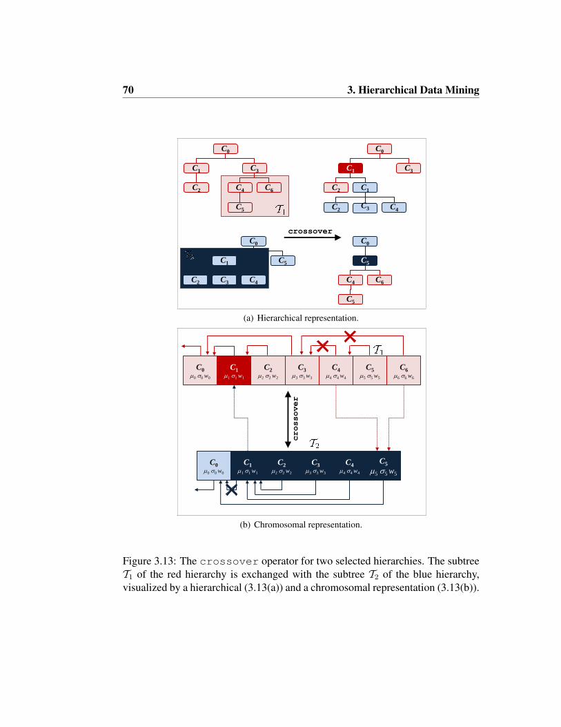
70 3. Hierarchical Data Mining
crossover
C0
C6
C5
C4
C3
C2
C1
C0
C1
C2 C3 C4
C5
C0
C1 C3
C2
C4
C5
C6
C0
C5
C1
C2C3 C4
(a) Hierarchical representation.
C00 0 w0
C11 1 w1
C22 2 w2
C33 3 w3
C44 4 w4
C66 6 w6
C55 5 w5
C00 0 w0
C11 1 w1
C22 2 w2
C33 3 w3
C44 4 w4
C5
5 5 w5
crossover
(b) Chromosomal representation.
Figure 3.13: The crossover operator for two selected hierarchies. The subtreeT1 of the red hierarchy is exchanged with the subtree T2 of the blue hierarchy,visualized by a hierarchical (3.13(a)) and a chromosomal representation (3.13(b)).

3.2 GACH: A Genetic Algorithm for Hierarchical Clustering 71
Fitness Function
Following Darwin‘s principle “Survival of the fittest” naturally only individualswith highest fitness can survive and those that are weaker become extinct. AGA adopts this aspect of evolution by the use of a fitness function. GACH usesthe hMDL criterion formalized in Section 3.1 which evaluates the fitness of achromosomal HCS by relating the clustering problem to that of data compressionby Huffman Coding. The authors define the coding scheme for a cluster hierarchyas follows:
hMDLHCS =∑
C∈HCS
(cost(C)− nWC log2(WC)− log2(
∑xvparent of C
Wx)
)
The coding cost for each cluster C ∈ HCS is determined separately and summedup to the overall coding cost of the complete HCS. Points that are directly as-signed to the cluster C together with the parameters µC and σC of the underlyingGaussian PDF are coded by cost(C). The point to cluster assignment is coded bythe so-called ID cost of each data point x ∈ C and is given by −nWC log2(WC)
where WC is the weight of cluster C and n the number of points. The binarylogarithm is used to represent the code length in bits. Clusters with higher weightare coded by a short code pattern whereas longer code patterns are assigned forsmaller clusters with lower weight. The ID costs for the parameters are formal-ized by− log2(
∑xvparent of C Wx) whereas constant ID costs are defined for the
parameters of the root node. The better the statistical model (the HCS) fits to thedata, the higher the compression rate, and thus the lower the coding costs. Usingthis coding scheme as fitness function ensures the selection of that chromosomeHCSChrom that fits best to the data.

72 3. Hierarchical Data Mining
Selection
The selection function chooses the best individuals out of a given set of individ-uals to form the offspring population w.r.t. their fitness. For GACH we use thewell-known weighted roulette wheel strategy [76]. Imagine that each HCSChromrepresents a number on a roulette wheel, where the amount of numbers refers tothe size of the population. In addition, we assign a weight to each number on theroulette wheel, depending on the fitness of the underlying chromosome, i.e. thebetter the fitness of a chromosome, the higher its weight on the roulette wheel,i.e. the higher the chance to get selected for the offspring population. Note thatthere is the chance that one chromosome is selected multiple times. GACH formsa new population that has as much individuals as the previous population.
Algorithmic Description
Now we are putting the pieces together to define the algorithmic procedure ofGACH, summarized in Algorithm 1. First, an initial population is built. This pop-ulation is evaluated according to the hMDL-based fitness function which meansthat GACH determines the coding cost for each cluster hierarchy of the popula-tion. In order to optimize the point to cluster assignment of each HCS and toprovide an additional model of the data, we apply a hierarchical EM algorithmon each cluster structure, as suggested for ITCH. That does not imply the typicalproblems of EM-based methods, as the model selection is performed by the ideaof GA. EM is only used to provide an additional feature in this case.
The population resulting from the initialization undergoes several mutationand crossover operations within popmax number of generations in an iterativeway. In each iteration the next population is selected according to the weightedroulette wheel strategy and experiences various reproduction procedures. Eachoperation is processed with a certain probability which is extensively evaluated inSection 3.2.2. After optimizing the point to cluster assignment, GACH determinesthe fitness of each HCSChrom. The algorithm terminates if a specified maximum

3.2 GACH: A Genetic Algorithm for Hierarchical Clustering 73
number of new populations popmax is reached. The experiments show that theHCS can be optimized even with a small number of generations.
Algorithm 1 GACH1: countpop ← 02: initialize population(countpop)3: evaluate population(countpop)4: while (countpop ≤ popmax) do5: countpop ← countpop + 16: select population(countpop) from population(countpop − 1)7: reproduce population(countpop)8: evaluate population(countpop)9: end while
3.2.2 Experimental Evaluation
Now we demonstrate that the genetic parameters (mutation rate, crossover rate andpopulation size) do not affect the effectiveness of GACH in a major way. Nev-ertheless, we provide a suitable parameterization that enables the user to receivegood results independent of the used dataset. Based on this, we compared theperformance of GACH to several representatives of various clustering paradigmson synthetic and real world data. We selected the most widespread approach tohierarchical clustering Single Link (SL) [53], the more outlier-robust hierarchicalclustering algorithm OPTICS [4] (requiring MinPts and ε), with optimal pa-rameters w.r.t. accuracy. Furthermore, we chose RIC [10], an outlier-robust andinformation-theoretic clusterer, and finally ITCH, introduced in Section 3.1, thatsuffers from the problem that the result only represents a local optimum in somecases. As ITCH depends on its initialization, we used the best out of ten runs inthis case.

74 3. Hierarchical Data Mining
Evaluation of Genetic Parameters
We applied GACH on two different datasets to evaluate the mutation and crossoverrates and the impact of the population size on the quality of the results w.r.t. thefitness function, introduced in Section 3.2.1. One dataset consists of 1,360 (2d)-data points that form a true hierarchy of six clusters. The second dataset covers850 (2d)-data points that are grouped in two flat clusters. For each experiment,we present the mean hMDL value and the corresponding standard deviation overten runs. GACH turned out to be very robust and determines very good clusteringresults (Prec > 90%, Rec > 90%) independent of the parameterizations.

3.2 GACH: A Genetic Algorithm for Hierarchical Clustering 75
Different Mutation Rates. We evaluated different mutation rates ranging from0.01 to 0.05 on two different population sizes and a fixed crossover rate of 0.15. Asa mutation is performed by one of the four operations delete, add, demoteor promote the mutation rate is the sum of pdel, padd, pdem and ppro (cf. Sec-tion 3.2.1). As demote and promote turned out to be essential for the qualityof the clustering results pdem and ppro are typically parameterized by a multiple ofpdel or padd due to the fact that the correct number of clusters is determined veryfast by the hMDL-based fitness function. However, finding the best HCS for agiven number of clusters is much more challenging. Figures 3.14(a) and 3.14(b)demonstrate that the mutation rate has no outstanding effect on the clustering re-sult, neither on a hierarchical nor on a flat dataset. Higher mutation rates result inhigher runtimes (3,388 ms for a mutation rate of 0.05 vs. 1,641 ms for a mutationrate of 0.01 on a hierarchical dataset, population size = 5). However, a highermutation rate provides more flexibility. Hence, we achieved slightly better resultswith a mutation rate of 0.05 (hMDL = 10, 520) compared to a mutation rate of0.01 (hMDL = 10, 542).
Different Crossover Rates. We compared different crossover rates pco rangingfrom 0.05 to 0.25 in combination with a mutation rate of 0.05 on two differentpopulation sizes. Figures 3.14(c) and 3.14(d) show that the performance of GACHis almost stable w.r.t. the different parameterizations of pco. Especially on a flatdataset a higher pco has no impact on the clustering result. GACH achieved anearly optimal hMDL value in almost every run, even for relatively small pop-ulation sizes. Higher pco values enable GACH to examine the search space moreeffectively as the crossover between two strong individuals produces an even fitterindividual. Therefore, we need fewer generations to find good clustering results,e.g. the result of GACH on the hierarchical dataset using five individuals was de-termined after 75 generations (1993 ms per generation) with pco = 0.05, and after61 generations (2,553 ms per generation) with pco = 0.25.

76 3. Hierarchical Data Mining
10600
10650
10700
MD
L va
lue
population size: 5 chromosomespopulation size: 20 chromosomes
10500
10550
0,01 0,02 0,03 0,04 0,05mea
n hM
mutation rate
(a) H: mutation rate
7540
7560
7580
7600
MD
L va
lue
population size: 5 chromosomespopulation size: 20 chromosomes
7500
7520
0,01 0,02 0,03 0,04 0,05mea
n hM
mutation rate
(b) F: mutation ratepopulation size: 5 chromosomespopulation size: 20 chromosomes
10700ue
population size: 20 chromosomes
10650
L va
l
10600
MD
L
10550
an h
M
105000,05 0,10 0,15 0,20 0,25m
ea
0,05 0,10 0,15 0,20 0,25
crossover rate
(c) H: crossover rate
population size: 5 chromosomespopulation size: 20 chromosomes
7600ue
population size: 20 chromosomes
7560
7580L
val
7540
7560M
DL
7520
an h
M
75000,05 0,10 0,15 0,20 0,25m
ea
0,05 0,10 0,15 0,20 0,25
crossover rate
(d) F: crossover rate
10700ue
10650
L va
l
10600
MD
L
10550
an h
M
105005 10 15 20 25m
ea
5 10 15 20 25
population size
(e) H: population size
7600ue
7560
7580
L va
l
7540
7560
MD
L
7520
an h
M
75005 10 15 20 25m
ea
5 10 15 20 25
population size
(f) F: population size
Figure 3.14: Mean fitness of resulting clusterings on (H)ierarchical and (F)latdatasets w.r.t. the genetic parameters mutation rate, crossover rate and populationsize.

3.2 GACH: A Genetic Algorithm for Hierarchical Clustering 77
Different Population Sizes. We tested the impact of the population size on thequality of the clustering result. We used populations that cover 5, 10, 15, 20 and25 hierarchical cluster structures in combination with a mutation rate of 0.05 anda crossover rate of 0.15. Figures 3.14(e) and 3.14(f) show again the mean hMDL
value over ten runs for each population size on two different datasets. Especiallythe plot of the hierarchical dataset demonstrates that a higher population size tendsto produce better results, which can be explained by the fact that a higher popula-tion size provides more variation opportunities whereby a global optimum can bereached easier. However, a large number of chromosomes cause a considerableamount of runtime. One generation using five chromosomes took 2462 ms on av-erage, the computation of a generation on 25 chromosomes took 9,229 ms. Hencewe use a population size consisting of ten cluster structures in combination with amutation rate of 0.05 and pco = 0.15 in the following experiments.
Competitive Performance of GACH
For these experiments we use two different synthetic datasets DS1 and DS2. DS1
is composed of 987 (2d)-data points that form a hierarchy of six clusters sur-rounded by local and global noise (cf. Figure 3.15(a)). DS2 consists of 1,950(2d)-data points that are grouped in three flat strongly overlapping clusters (cf.Figure 3.15(b)). For each dataset, the clustering results were assessed against aground-truth classification and evaluated the results w.r.t. six different validitymeasures: the recently proposed information-theoretic methods [77] NormalizedMutual Information (NMI), Adjusted Mutual Information (AMI) and ExpectedMutual Information (EMI). All these measures have a maximum value of 1 (whichrefers to a perfect clustering) and a minimum value of 0. Furthermore, we chosethe well-known Precision (Prec) and Recall (Rec) and the DOM [30] value thatreflects the coding costs to encode the class labels when the cluster labels areknown, i.e. low DOM values represent good clustering results.

78 3. Hierarchical Data Mining
Evaluation w.r.t. Dataset D1. These experiments demonstrate that GACH per-forms at least as good as the parameter dependent approach OPTICS (MinPts =
6, ε = 0.9) and ITCH, while being much more accurate than RIC and SL. Thereachability plot of OPTICS is provided in Figure 3.15(c), the SL dendrogram isshown in Figure 3.15(e). Although DS1 seems to be an easy to cluster dataset, SLand RIC fail in assigning the local and global outliers to the correct cluster. Both,GACH and ITCH were able to determine the right cluster structure. However,GACH outperformed ITCH w.r.t. accuracy, as GACH results in a different pointsto clusters assignment. Therefore, GACH shows the best performance on DS1
concerning the information-theoretic measures NMI, AMI and EMI. 94% of alldata points are assigned to the true cluster and 95% of the cluster contents weredetected correctly by GACH. Finally, this result can be coded most efficiently asstated by the low DOM value of 0.4193. This evaluation is summarized in Ta-ble 3.5.
Table 3.5: Performance of GACH on DS1.
GACH ITCH RIC OPTICS SLNMI 0.9346 0.9265 0.8673 0.9045 0.9110AMI 0.9159 0.8999 0.7678 0.8662 0.8997EMI 0.0004 0.0004 0.0004 0.0004 0.0002PREC 0.9404 0.9222 0.6438 0.8626 0.9555REC 0.9514 0.9422 0.7720 0.9200 0.9169DOM 0.4193 0.4454 0.6638 0.4960 0.4765
Evaluation w.r.t. Dataset D2. Neither OPTICS nor SL were able to detect thetrue cluster structure of DS2. Both fail because of a massive Single Link effectand therefore the reachability plot provided by OPTICS (cf. Figure 3.15(d)) andthe dendrogram produced by SL (cf. Figure 3.15(f)) do not uncover any clusterstructure which leads to a clustering where all objects belong to one single clus-ter. RIC determines only one single cluster. ITCH separates the two red Gaus-sian clusters but fails in assigning the data points generated by the blue cluster

3.2 GACH: A Genetic Algorithm for Hierarchical Clustering 79
2 clusters with local noise
2 clusters with
global noise
local noise 2 clusters with local noise
(a) Plotted DS1. (b) Plotted DS2.
Cut w.r.t. reachability distance = 0.07
2 clusters with local
noise
2 clusters with local
noise
2 clusters with local
noise
(c) OPTICS on DS1. (d) OPTICS on DS2.
Cutoff value = 0.9
(e) SL on DS1. (f) SL on DS2.
Figure 3.15: Competitive evaluation of GACH on two different synthetic datasets.DS1 forms a hierarchy including local and global noise, DS2 is a flat dataset ofthree overlapping clusters.

80 3. Hierarchical Data Mining
correctly. Hence, GACH turned out to be the only algorithm that handles thisdatasets with strongly overlapping clusters successfully. It shows the best valuesw.r.t. information-theoretic criterions, while being very accurate. Its result causesonly a coding cost of 0.3325 compared to more than 0.9 for almost all other ap-proaches. This is summarized in Table 3.6.
Table 3.6: Performance of GACH on DS2.
GACH ITCH RIC OPTICS SLNMI 0.6698 0.6316 0.0000 0.0000 0.0000AMI 0.5877 0.4030 0.0000 0.0000 0.0000EMI 0.1476 0.2256 0.2379 0.2379 0.2379PREC 0.9184 0.8227 0.2130 0.2130 0.2130REC 0.9226 0.8913 0.4615 0.4615 0.4615DOM 0.3325 0.4226 0.9184 0.9184 0.9184
Application of GACH on Real World Data
We tested the practical application of GACH on the Wine dataset, available atUCI2. This dataset contains 178 (13-d)-data objects resulting from a chemicalanalysis of wines grown in the same region in Italy but derived from three differentcultivars. The dataset provides a ground-truth classification that structures the datainto one root node covering the whole dataset and three subclusters defining thethree cultivars. GACH determined this structure resulting in high validity values.
The competitors did not even find the right number of clusters. OPTICS, forexample detects two clusters (cf. Figure 3.16(a)) and RIC even merges all datapoints in only one single cluster. The hierarchy of SL covers four disjoint clustersw.r.t. a cutoff value of 40. These results demonstrate that GACH finds a globaloptimum w.r.t. accuracy in real world data and is therefore applicable in manydomains.
2http://archive.ics.uci.edu/ml/datasets/Wine

3.2 GACH: A Genetic Algorithm for Hierarchical Clustering 81
Cut w.r.t. reachability distance = 0.5
1 large cluster 1 smaller cluster
(a) OPTICS on Wine.
Cutoff value = 40
(b) SL on Wine.
Figure 3.16: Competitive evaluation of GACH on the real-world Wine dataset.
Table 3.7: Performance of GACH on the real-world Wine dataset.
GACH ITCH RIC OPTICS SLNMI 0.7886 0.7615 0.0000 0.5079 0.3852AMI 0.7813 0.6912 0.0000 0.4817 0.3485EMI 0.0013 0.0014 0.0000 0.0013 0.0018PREC 0.9401 0.9737 0.1591 0.7466 0.5309REC 0.9326 0.8596 0.3989 0.6966 0.5337DOM 0.3631 0.3285 1.1405 0.6853 1.0740
3.2.3 Conclusions
We proposed a genetic algorithm for finding cluster hierarchies, called GACH.GACH combines the benefits of genetic algorithms, information theory and model-based clustering. As GACH uses a MDL-based fitness function, it can be easilyapplied to real world applications without requiring any expertise about the data.Due to the fact that GACH integrates an EM-like strategy, the content of all clus-ters is described by an intuitive description. Outliers are assigned to appropriateinner nodes.

82 3. Hierarchical Data Mining

Chapter 4
Integrative Data Mining
Integrative mining of heterogeneous data is one of the grand challenges for datamining in the next decade. Recently, the need for integrative data mining tech-niques has been emphasized in panel discussions, e.g. at KDD 2006 [83], in work-shops [109], and in position papers [108, 59]. Integrative data mining is amongthe top ten challenging problems in data mining identified in [108]. Moreover itis essential for solving many of the other top 10 challenges, including data miningin social networks and data mining for biological and environmental problems.
4.1 INTEGRATE: A Clustering Algorithm for Het-erogeneous Data
We address the question of how to find a natural clustering of data with mixedtype attributes. In everyday life, huge amounts of such data are collected, forexample from credit assessments. The collected data include numerical attributes,such as credit amount and age, as well as categorical attributes, such as personalstatus and the purpose of the credit. A cluster analysis of credit assessment datais interesting, e.g., for target marketing. We could give numerous more examplesfor data with mixed type attributes from various applications including medical,

84 4. Integrative Data Mining
bioinformatics and web usage. However, finding a natural clustering of such datais a non-trivial task. We identified two major problems:
• Problem 1: Much previous knowledge required.
• Problem 2: No adequate support of mixed type attributes.
To cope with these two major problems, we propose INTEGRATE, a parameter-free technique for integrative clustering of data with mixed type attributes. Themajor benefits of our approach can be summarized as follows:
1. Natural balance of numerical and categorical information in clustering sup-ported by information theory;
2. Parameter-free clustering;
3. Making most effective usage of numerical as well as categorical informa-tion;
4. Scalability to large datasets.
4.1.1 Minimum Description Length for Integrative Clustering
Notations. In the following we are considering a datasetDS with n objects. Eachobject x is represented by d attributes. Attributes are denoted by capital letters andcan be either numerical features or categorical variables with two or more values.For a categorical attribute A, we denote a possible value of A by a. The result ofour algorithm is a disjoint partitioning of DS into k clusters C1, · · · , Ck.
Likelihood and Data Compression. One of the most challenging problems inclustering data with mixed type attributes is selecting a suitable distance function,or unifying clustering results obtained on the different representations of the data.Often, the weighting between the different attribute types needs to be specified by

4.1 INTEGRATE: A Clustering Algorithm for Heterogeneous Data 85
parameter settings, cf. Section 2.2. The minimum description length (MDL) prin-ciple provides an attractive theoretical foundation for parameter-free integrativeclustering avoiding this problem. Recently, the MDL-principle and related ideashave been successfully applied to avoid crucial parameter settings in clusteringvector data. For hierarchical data mining we contributed hMDL (cf. Section 3.1),but to the best of our knowledge MDL has not been applied to integrative cluster-ing so far. Also for heterogeneous data, it is very beneficial to regard clustering asa data compression problem, naturally balancing the influence of categorical andnumerical attributes.
Coding Categorical Data
To give a simple example, assume we need to transfer 1,000 1-dimensional cate-gorical data objects. Each object is represented by a categorical attribute A withtwo possible values {red, blue}. It can be shown that the code length to transferthis data is lower bounded by the entropy of the attribute A. Thus, the codingcosts CC of attribute A are provided by:
CC(A) = −∑a∈A
p(a) · log2 p(a).
Here, a denotes each possible value or outcome of the categorical attribute. By theapplication of the binary logarithm we obtain the code length in bits. If we haveno additional knowledge on the data we have to assume that the probabilities forred and blue are both 0.5. With this assumption, we need one bit to encode eachdata object and the communication costs would be 1,000 bits. Clustering, how-ever, provides high-level knowledge on the data which allows for a much moreeffective way to reduce the communication costs. Even if the probabilities for thedifferent outcomes of the categorical attributes are approximately equal consider-ing the whole dataset, often different clusters with non-uniform probabilities canbe found.

86 4. Integrative Data Mining
10
8
6
44
2
0 x-2 -1 0 1 2 3 4 5-3-4
Figure 4.1: Top: Example dataset with two numerical and one categorical attributewith the outcomes red and blue. Bottom: Cost curves assuming two clusters:Considering the numerical information only (green), integrating numerical andcategorical information (red, blue). For each outcome and each cluster, we have aunique cost curve. Intersection points mark the resulting cluster borders.
As an example, refer to the data displayed in Figure 4.1. The data is representedby two numerical attributes that will be taken into account in the next paragraph,and one categorical attribute. The categorical attribute has two possible values,red and blue, which are visualized by the corresponding colors. Considering alldata, the probabilities for red and blue are both 0.5. However, it is evident thatthe outcomes red and blue are not uniformly distributed in all areas of the dataspace. Rather, we have two clusters, one mainly hosts the red objects, and theother the blue ones. In fact, the data has been generated such that in the clusterdisplayed on the left, we have 88% of blue objects and 12% of red objects. Forthe cluster on the right, the ratio has been selected reciprocally. This clusteringdrastically reduces the entropy and therefore the coding costs of the categoricalattribute to CC(A) = 0.53 bits per data object, which corresponds to the entropyof A in both clusters. However, we would need to transfer the clustering result

4.1 INTEGRATE: A Clustering Algorithm for Heterogeneous Data 87
itself, including the cluster identifiers to the receiver. Before discussing how toencode the clustering result, we will consider how to encode numerical data.
Coding Numerical Data
If our dataset contains an additional numerical attribute B we can also use therelationship between likelihood and data compressibility to reduce the communi-cation costs. To specify the probability of each data object considering attributeB, we assign a probability density function (PDF) to B. Here, we apply a Gaus-sian PDF for each numerical attribute. However, let us note that our ideas canbe straightforwardly extended to other types PDF, e.g. Laplacian or GeneralizedGaussian. Thus, the probability density function of a numerical attribute B isprovided by:
p(b) =1
σ√
2πexp
(−(b− µB)2
2σ2B
).
If the data distribution of attribute B is Gaussian with mean µB and standard de-viation σB, we minimize the communication costs of the data by a coding schemewhich assigns short bit strings to objects with coordinate values that are in thearea of high probability and longer bit strings to objects with lower probabilityaccording to the idea of Huffman-Coding. Let us note that we do not considerhow to actually construct such code. Rather, we are interested in the code lengthas a measure for clustering quality. The coding costs of attribute B are providedby:
CC(B) = −∫p(b) log2 p(b)db.
Again, if we have no knowledge on the data, we would have to assume that eachattribute is represented by a single Gaussian with mean and standard deviationdetermined from all data objects. As discussed for categorical data, clusteringcan often drastically reduce the communication costs. Most importantly, relat-ing clustering to data compression allows us a unified view on data with mixed

88 4. Integrative Data Mining
type attributes. Consider again the data displayed in Figure 4.1. In addition tothe categorical attribute we now consider the numerical x-coordinate, denoted byX . To facilitate presentation, we ignore the y-coordinate which is processed anal-ogously. The two green curves at the bottom represent the coding costs of thetwo clusters considering X . For both curves, the cost minimum coincides withthe mean of the Gaussian which generated the data. The cluster on the right hasbeen generated with slightly larger variance, resulting in slightly higher codingcosts. The intersection of both cost curves represents the border between the twoclusters provided by X , indicated by a green vertical line. In addition, for eachcluster and each outcome of the categorical attribute, we have included a costcurve (displayed in the corresponding colors). Again, the intersection points markthe cluster borders provided by the categorical attribute. Consider, e.g., the redvertical line. Red objects with a value in X beyond that point are assigned to thecluster on the right. Thus, in the area between the red and the blue vertical line,the categorical value is the key information for clustering. Note that all bordersare not fixed but optimized during the run of our algorithm.
A Coding Scheme for Integrative Clustering
As mentioned, in addition to the coding costs for categorical and numerical at-tributes of the data objects, we need to elaborate a coding scheme describing theclustering result itself. The additional coding costs for encoding the clusteringresult can be classified into two categories: the parameter costs required to spec-ify the cluster model and the id-costs required to specify the cluster-id for eachobject, i.e. the information to which cluster the object belongs.
For the parameter costs, we focus on the set of objects belonging to a singlecluster C. To specify the cluster model, we need for each categorical attribute Ato encode the probability of each value or outcome a. For a categorical attributewith |A| possible values, we need to encode |A|−1 probabilities since the remain-ing probability is implicitly specified. For each numerical attribute B we need toencode the parameters µB and σB of the PDF. Following a central result from the
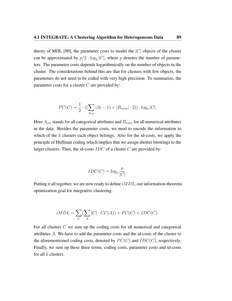
4.1 INTEGRATE: A Clustering Algorithm for Heterogeneous Data 89
theory of MDL [90], the parameter costs to model the |C| objects of the clustercan be approximated by p/2 · log2 |C|, where p denotes the number of parame-ters. The parameter costs depends logarithmically on the number of objects in thecluster. The considerations behind this are that for clusters with few objects, theparameters do not need to be coded with very high precision. To summarize, theparameter costs for a cluster C are provided by:
PC(C) =1
2· ((∑Acat
|A| − 1) + |Bnum| · 2)) · log2 |C|.
HereAcat stands for all categorical attributes andBnum for all numerical attributesin the data. Besides the parameter costs, we need to encode the information towhich of the k clusters each object belongs. Also for the id-costs, we apply theprinciple of Huffman coding which implies that we assign shorter bitstrings to thelarger clusters. Thus, the id-costs IDC of a cluster C are provided by:
IDC(C) = log2
n
|C|.
Putting it all together, we are now ready to define iMDL, our information-theoreticoptimization goal for integrative clustering.
iMDL =∑C
(∑A
|C| · CC(A)) + PC(C) + IDC(C).
For all clusters C we sum up the coding costs for all numerical and categoricalattributes A. We have to add the parameter costs and the id-costs of the cluster tothe aforementioned coding costs, denoted by PC(C) and IDC(C), respectively.Finally, we sum up these three terms, coding costs, parameter costs and id-costsfor all k clusters.

90 4. Integrative Data Mining
4.1.2 The Algorithm INTEGRATE
Now we present the highly effective k-means based algorithm INTEGRATE forclustering mixed type attributes that is based on the MDL-based criterion iMDL,defined in Section 4.1.1. INTEGRATE is designed to find the optimal clusteringof a dataset DS, where each object x comprises both numerical and categoricalattributes by optimizing the overall compression rate. First, INTEGRATE buildsan initial partitioning of k clusters. Each cluster is represented by a Gaussian PDFin each numerical dimension B with µB and σB, and a probability for each valueof the categorical attributes. All objects are then assigned to the k clusters by min-imizing the overall coding costs iMDL. In the next step, the parameters of eachcluster are recalculated according to the assigned objects. That implies µ and σin each numerical dimension and the probabilities for each value of the categori-cal attributes, respectively. After initialization the following steps are performedrepeatedly until convergence. First, the costs for coding the actual cluster parti-tion are determined. Second, the assignment of objects to clusters is performedin order to decrease the iMDL value. Third, the new parameters of each clusterare recalculated. INTEGRATE terminates if no further changes of cluster assign-ments occur. Finally, we receive the optimal clustering for DS represented by kclusters according to minimum coding costs.
Initialization
The effectiveness of an algorithm often heavily depends on the quality of the ini-tialization, as it is the case that many algorithms can get stuck in a local optimum.Hence, we propose an initialization scheme to avoid this effect. We have to findinitial cluster representatives that correspond best to the final representatives. Anestablished method for partitioning methods is to initialize with randomly chosenobjects of DS. We adopt this idea and take the µ of the numerical attributes ofk randomly chosen objects as cluster representatives. During initialization, weset σ = 1.0 in each numerical dimension. The probabilities of the values for the
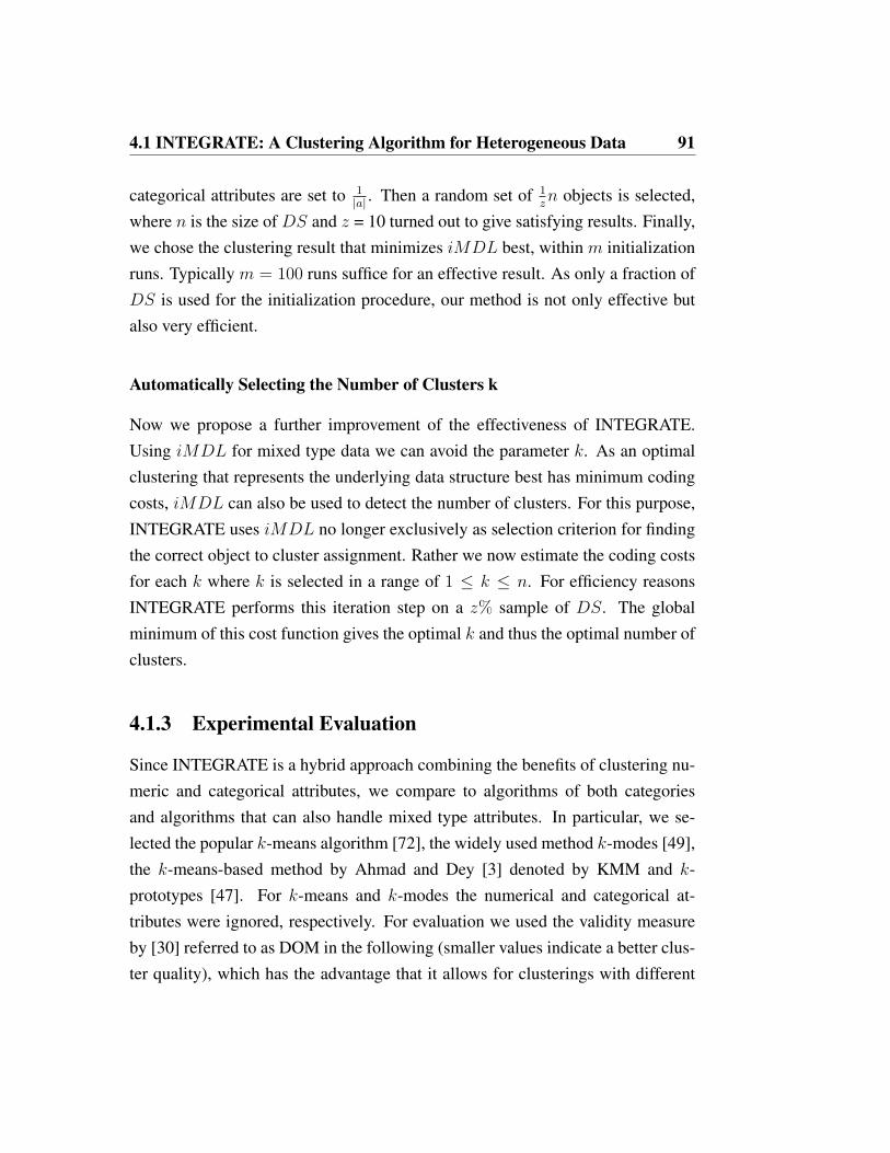
4.1 INTEGRATE: A Clustering Algorithm for Heterogeneous Data 91
categorical attributes are set to 1|a| . Then a random set of 1
zn objects is selected,
where n is the size of DS and z = 10 turned out to give satisfying results. Finally,we chose the clustering result that minimizes iMDL best, within m initializationruns. Typically m = 100 runs suffice for an effective result. As only a fraction ofDS is used for the initialization procedure, our method is not only effective butalso very efficient.
Automatically Selecting the Number of Clusters k
Now we propose a further improvement of the effectiveness of INTEGRATE.Using iMDL for mixed type data we can avoid the parameter k. As an optimalclustering that represents the underlying data structure best has minimum codingcosts, iMDL can also be used to detect the number of clusters. For this purpose,INTEGRATE uses iMDL no longer exclusively as selection criterion for findingthe correct object to cluster assignment. Rather we now estimate the coding costsfor each k where k is selected in a range of 1 ≤ k ≤ n. For efficiency reasonsINTEGRATE performs this iteration step on a z% sample of DS. The globalminimum of this cost function gives the optimal k and thus the optimal number ofclusters.
4.1.3 Experimental Evaluation
Since INTEGRATE is a hybrid approach combining the benefits of clustering nu-meric and categorical attributes, we compare to algorithms of both categoriesand algorithms that can also handle mixed type attributes. In particular, we se-lected the popular k-means algorithm [72], the widely used method k-modes [49],the k-means-based method by Ahmad and Dey [3] denoted by KMM and k-prototypes [47]. For k-means and k-modes the numerical and categorical at-tributes were ignored, respectively. For evaluation we used the validity measureby [30] referred to as DOM in the following (smaller values indicate a better clus-ter quality), which has the advantage that it allows for clusterings with different

92 4. Integrative Data Mining
numbers of clusters and integrates the class labels as “ground truth”. In each ex-periment, we report the average performance of all clustering algorithms over tenruns.
Synthetic Data
If not specified otherwise, the artificial datasets include three Gaussian clusterswith each object having two numerical and one categorical attribute. To validatethe results we added a class label to each object which was not used for clustering.
Varying Ratio of Categorical Attribute Values. We generated 3-dimensionalsynthetic datasets with 1,500 points including two numerical and one two-valuedcategorical attribute. We varied the ratio for each categorical attribute value from0% to 100% clusterwise in each dataset. Without need for difficult parameter set-ting our proposed method performs best in all cases (cf. Figure 4.2(a)). Even inthe case of equally (50%) distributed values, where the categorical attribute givesno information for separating the objects, the cluster quality of INTEGRATE isbest compared to all other methods. As k-means does not take the categoricalattributes into account the performance is relatively constant.
Varying Variance of Clusters. This experiment aims at comparing the perfor-mance of the different methods on datasets with varying variances. In particular,we generated synthetic datasets each comprising 1,500 points including two nu-merical and one two-valued categorical attribute that form three Gaussian clusterswith a variance ranging from 0.5 to 2.0. Figure 4.2(b) shows that INTEGRATEoutperforms all competitors in all cases, in which each case reflects different de-gree of overlap of the three clusters. Even at a variance of 2.0 where the numeri-cal attributes carry nearly no cluster information our proposed method shows bestcluster quality. In this case the categorical attributes are used to separate the clus-ters. On the contrary, k-modes performs worst as it can only use the categoricalattribute as single source for clustering.
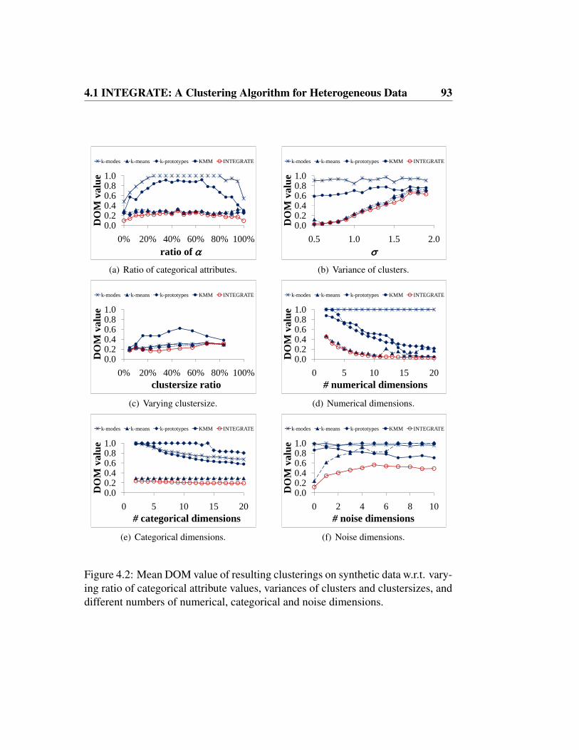
4.1 INTEGRATE: A Clustering Algorithm for Heterogeneous Data 93
0 60.81.0
valu
e
k-modes k-means k-prototypes KMM INTEGRATE
0.00.20.40.6
0% 20% 40% 60% 80% 100%
DO
M v
ratio of α
(a) Ratio of categorical attributes.
0 60.81.0
valu
e
k-modes k-means k-prototypes KMM INTEGRATE
0.00.20.40.6
0.5 1.0 1.5 2.0
DO
M v
σ
(b) Variance of clusters.
0 60.81.0
valu
e
k-modes k-means k-prototypes KMM INTEGRATE
0.00.20.40.6
0% 20% 40% 60% 80% 100%
DO
M v
clustersize ratio
(c) Varying clustersize.
0 60.81.0
valu
ek-modes k-means k-prototypes KMM INTEGRATE
0.00.20.40.6
0 5 10 15 20
DO
M v
# numerical dimensions
(d) Numerical dimensions.
0 60.81.0
valu
e
k-modes k-means k-prototypes KMM INTEGRATE
0.00.20.40.6
0 5 10 15 20
DO
M v
# categorical dimensions
(e) Categorical dimensions.
0 60.81.0
valu
e
k-modes k-means k-prototypes KMM INTEGRATE
0.00.20.40.6
0 2 4 6 8 10
DO
M v
# noise dimensions
(f) Noise dimensions.
Figure 4.2: Mean DOM value of resulting clusterings on synthetic data w.r.t. vary-ing ratio of categorical attribute values, variances of clusters and clustersizes, anddifferent numbers of numerical, categorical and noise dimensions.

94 4. Integrative Data Mining
Varying Clustersize. In order to test the performance of the different methodson datasets with unbalanced clustersize we generated three Gaussian clusters withdifferent variance and varied the ratio of number of points per cluster from 0% to100% in five steps. It is obvious from Figure 4.2(c) that INTEGRATE separatesthe three clusters best even with highly unbalanced cluster sizes. Only in the caseof two very small clusters and one big cluster k-modes shows a slightly bettercluster validity.
Varying Number of Numerical Dimensions. In this experiment we leave thenumber of categorical attributes to a constant value and successively add numer-ical dimensions to each object that are generated with a variance of σ=1.8. IN-TEGRATE shows best performance in all cases (cf. Figure 4.2(d)). All methodsshow a slight increase in cluster quality when varying the numerical dimensional-ity, except k-modes that performs constantly as it does not consider the numericalattributes.
Varying Number of Categorical Dimensions. For each object we added three-valued categorical attributes where we set the probability of the first value to 0.6
and the probability of the two remaining values to 0.2, respectively. Figure 4.2(e)illustrates that our proposed method outperforms the other methods and even k-modes by magnitudes which is a well-known method for clustering categoricaldata. Whereas KMM shows a heavy decrease in clustering quality in the caseof two and four additional categorical attributes, our method performs relativelyconstant. Taking the numerical attributes not into account the cluster validity ofk-means remains constant.
Noise Dimensions. Figure 4.2(f) illustrates the performance of the different meth-ods on noisy data. It is obvious that INTEGRATE outperforms all compared meth-ods when adding non-clustered noise dimensions to the data. k-means shows a
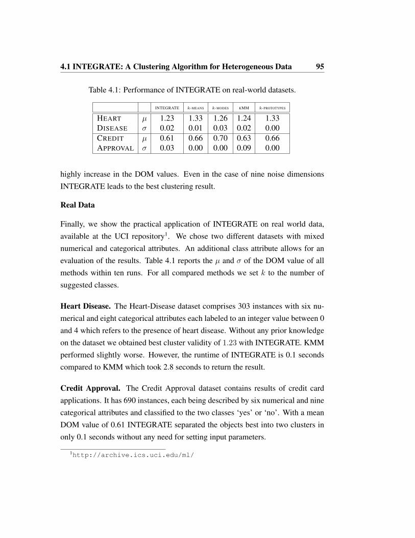
4.1 INTEGRATE: A Clustering Algorithm for Heterogeneous Data 95
Table 4.1: Performance of INTEGRATE on real-world datasets.
INTEGRATE k-MEANS k-MODES KMM k-PROTOTYPES
HEART µ 1.23 1.33 1.26 1.24 1.33DISEASE σ 0.02 0.01 0.03 0.02 0.00CREDIT µ 0.61 0.66 0.70 0.63 0.66APPROVAL σ 0.03 0.00 0.00 0.09 0.00
highly increase in the DOM values. Even in the case of nine noise dimensionsINTEGRATE leads to the best clustering result.
Real Data
Finally, we show the practical application of INTEGRATE on real world data,available at the UCI repository1. We chose two different datasets with mixednumerical and categorical attributes. An additional class attribute allows for anevaluation of the results. Table 4.1 reports the µ and σ of the DOM value of allmethods within ten runs. For all compared methods we set k to the number ofsuggested classes.
Heart Disease. The Heart-Disease dataset comprises 303 instances with six nu-merical and eight categorical attributes each labeled to an integer value between 0and 4 which refers to the presence of heart disease. Without any prior knowledgeon the dataset we obtained best cluster validity of 1.23 with INTEGRATE. KMMperformed slightly worse. However, the runtime of INTEGRATE is 0.1 secondscompared to KMM which took 2.8 seconds to return the result.
Credit Approval. The Credit Approval dataset contains results of credit cardapplications. It has 690 instances, each being described by six numerical and ninecategorical attributes and classified to the two classes ‘yes’ or ‘no’. With a meanDOM value of 0.61 INTEGRATE separated the objects best into two clusters inonly 0.1 seconds without any need for setting input parameters.
1http://archive.ics.uci.edu/ml/

96 4. Integrative Data Mining
Finding the optimal k
By means of the dataset illustrated in Figure 4.3(a), we highlight the benefit ofINTEGRATE for finding the correct number of clusters. The dataset comprisessix Gaussian clusters, where each object has two numerical and one categorical at-tribute with two different values that are marked in “red” and “blue”. Figure 4.3(b)shows the iMDL value of the data model for different values of k. The cost func-tion has its global minimum, which refers to the optimal number of clusters, atk = 6. In the range of 1 ≤ k ≤ 4 the plotted function shows an intense de-crease in the coding costs and for k > 6 a slight increase of the coding costs asin these cases the data does not optimally fit into the model and therefore causeshigh costs. Note, that there is a local minimum at k = 4, which would also referto a meaningful number of clusters.
(a) The dataset. (b) iMDL for 1 ≤ k ≤ 30.
Figure 4.3: Coding costs for different k according to a dataset of six clusters.
4.1.4 Conclusions
We addressed integrative clustering of data covering both numerical and cate-gorical attributes. In addition, we gave in a solution to avoid difficult parametersettings, guided by the idea of data compression. On top of that concept, we haveproposed INTEGRATE, an information-theoretic integrative clustering method,that allows for a natural weighting of numerical and categorical information. Inaddition, INTEGRATE is fully automatic and shows high efficiency and is there-fore scalable to large datasets.

Chapter 5
Mining Skyline Objects
Skyline queries are an important area of current database research, and havegained increasing interest in recent years [19, 93, 58]. Most papers focus on effi-cient algorithms for the construction of a single skyline which is the answer of auser’s query. We extend the idea of skylines in such a way that multiple skylinesare treated as objects for data exploration and data mining.
5.1 SkyDist: An Effective Similarity Measure forSkylines
One of the most prominent applications of the skyline operator is to support com-plex decisions. As an example consider an online marketplace for used cars,where the user wants to find out offers which optimize more than one propertyof the car such as p (price) and m (mileage), with an unknown weighting of thesingle conditions. The result of such a query has to contain all offers which maybe of interest: not only the cheapest offer and that with lowest mileage but alsoall offers providing an outstanding combination of p and m. This concept is illus-trated in Figure 5.1(a) which displays a set of database objects representing all caroffers (lets say for an Audi A3 1.6) described by the attributes p and m. However,

98 5. Mining Skyline Objects
G
m
p
Skyline of Audi A3 1.6 A
(a) Database objects andtheir skyline.
BMW 7 3.0
Audi A8 3.3
Ford Focus 1.6
Audi A3 1.6
p
m
(b) Skylines of differentcar models.
(c) A 3-dimensional skyline.
Figure 5.1: Motivating examples for performing data mining on skylines.
not all of these offers are equally attractive to the user. For instance, offer A hasboth a lower price and a lower mileage than G and many other offers. Therefore,we say that A dominates G (in symbols A ≺ G), because A is better than G w.r.t.any possible weighting of the criteria price and mileage. The skyline containsall objects which are not dominated by any other object in the database. In Fig-ure 5.1(a), the skyline objects exhibiting an outstanding combination of price andmileage are highlighted in red.
For the used car market, the skyline of each car model has a particular mean-ing: Many arbitrarily bad offers may be present in the database but only the offersin (or close to) the skyline have a high potential to find a customer. The skylineof the offers marks to some degree the fair value of a car for each mileage in themarket. Therefore, the skyline characterizes a car model (or higher-order objectsof other applications) in a highly expressive way.
This high expressiveness leads us to the idea of treating the skylines them-selves as objects with the corresponding similarity measure, called SkyDist. Fig-ure 5.1(b) illustrates the skylines of four different car models derived from anonline automotive market. Car models which exhibit similar skylines (like AudiA3 1.6 and Ford Focus 1.6) may be considered as similar: A recommender systemmight find out that the Focus is a perfect alternative to the Audi A3. The differentcar models may be subject to clustering, classification, outlier detection, or othersupervised or unsupervised data mining tasks, using a similarity measure which is

5.1 SkyDist: An Effective Similarity Measure for Skylines 99
built upon the skyline.Since the different 2-dimensional skylines in Figure 5.1(b) look like well-knownstructures (like time series or trajectories), we may gain the impression that ap-propriate techniques could be helpful for the definition of the skyline similarity.However, when taking a closer look at a skyline in a 3- or higher dimensional dataspace as shown in Figure 5.1(c) with the attributes p (price), m (mileage), and a(age), it becomes obvious that this is not sufficient. Unfortunately, there existsno natural dimension which can be used for ordering the skyline objects. There-fore, our solution is based on a different concept, namely the symmetric volumedifference of the two skylines to be compared.
5.1.1 SkyDist
At the beginning of this section we define the essential concepts underlying Sky-Dist in general. Then we motivate the idea behind assigning SkyDist for 2-dimensional skylines and conclude with a generalization according d-dimensionalskylines, where d ≥ 2.
Theoretical Background
Consider a set of database objects, each of which is already associated with anindividual skyline. For instance, each car type is associated with the skyline ofthe offers posted in a used car market. An effective distance measure for a pair ofskyline objects should be useful in the sense that the characteristic properties ofthe skyline concept are suitably reflected. Whenever two skylines are similar inan intuitive sense, then SkyDist should yield a small value. In order to define sucha reasonable distance measure, we recall here the central concept of the classicalskyline operator, the dominance relation which can be built on the preferences onattributes D1, . . . ,Dd in a d-dimensional numeric space D.
Definition 4 (Dominance) For two data points u and v, u dominates v, denoted
by u ≺ v, if the following two conditions hold:

100 5. Mining Skyline Objects
∀ dimensions Di∈{1,...,d}: u.Di ≤ v.Di∃ dimension Dj∈{1,...,d}: u.Dj < v.Dj .
Definition 5 (Skyline Point / Skyline) Given a set of data points DS, a data
point u is a skyline point if there exists no other data point v ∈ DS such that
v dominates u. The skyline on DS is set of size s containing all skyline points.
Two skylines are obviously equal when they consist of identical points. Intu-itively, one can say that two skylines are similar, whenever they consist of similarpoints. But in addition, two skylines may also be considered similar if they dom-inate approximately the same points in the data space. This can be grasped in asimple and efficient way by requiring that the one of the two skylines should notchange much whenever the points of the other skyline are inserted into the firstone and vice versa. This leads us to the idea to base SkyDist on the set-theoreticdifference among the parts of the data space which are dominated by the twoskylines. For a more formal view let us define the terms dominance region andnon-dominance region of a skyline.
Definition 6 (Dominance Region of a Skyline Point) Given a skyline point
xi∈{1,...,s} of a skyline X = {x1, . . . , xs}. The dominance region of xi, denoted
by DOMxi , is the data space, where every data point u ∈ DOMxi complies the
condition xi ≺ u.
Definition 7 (Dominance Region of a Skyline) Given the set of all skyline points
of a skyline X . The dominance region of the skyline X , denoted by DOMX , is
defined over the union of the dominance regions of all skyline points xi∈{1,...,s}.
Figure 5.2 illustrates this notion for two given skylines X and Y . The green andblue areas show the dominance regions of skylines X and Y , respectively.
Definition 8 (Non-Dominance Region of a Skyline) Given a numeric spaceD =
(D1, . . . ,Dd) and the dominance regionDOMX of a skylineX . The non-dominanceregion of X , denoted by DOMX , is D \ DOMX .
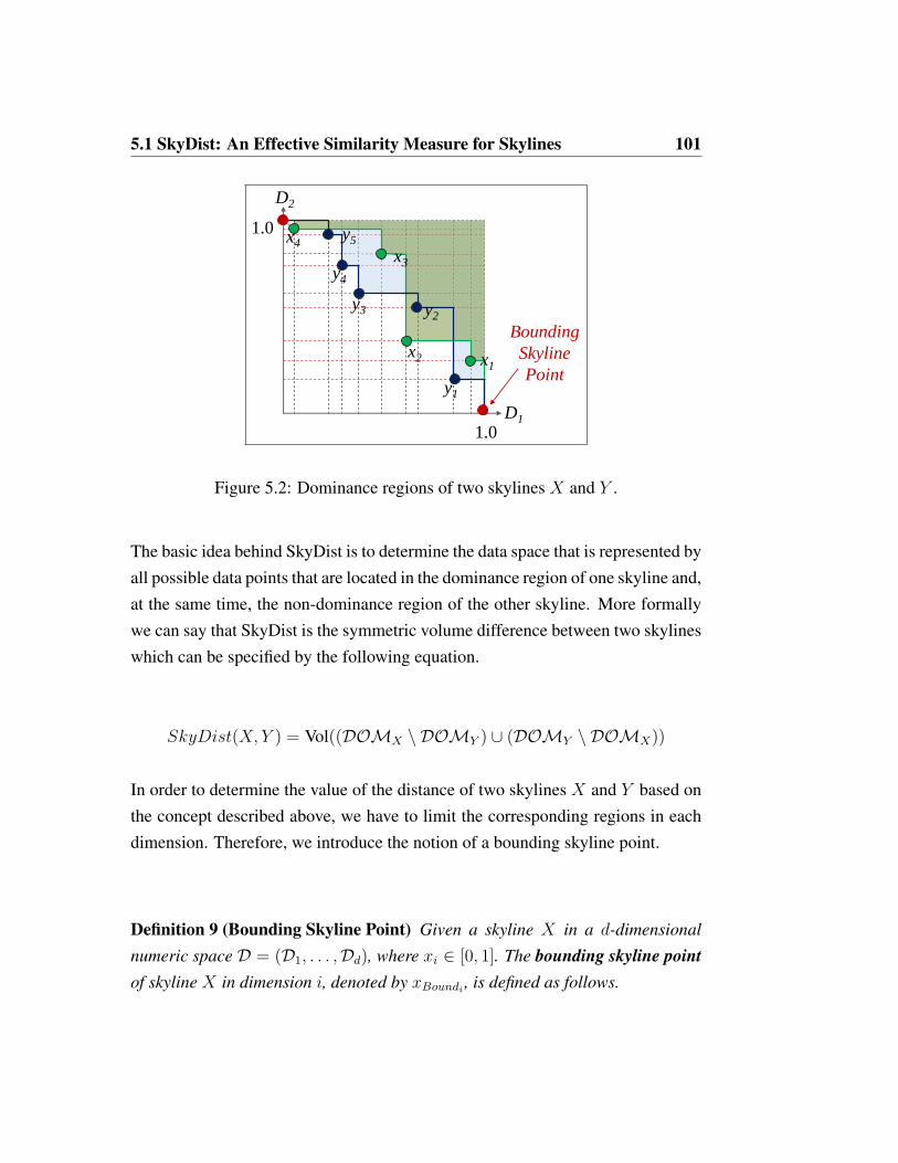
5.1 SkyDist: An Effective Similarity Measure for Skylines 101
1.0
1.0
D1
D2
x2
x4
y4
y3 y2
y1
y5
x3
x1
Bounding
Skyline
Point
Figure 5.2: Dominance regions of two skylines X and Y .
The basic idea behind SkyDist is to determine the data space that is represented byall possible data points that are located in the dominance region of one skyline and,at the same time, the non-dominance region of the other skyline. More formallywe can say that SkyDist is the symmetric volume difference between two skylineswhich can be specified by the following equation.
SkyDist(X, Y ) = Vol((DOMX \ DOMY ) ∪ (DOMY \ DOMX))
In order to determine the value of the distance of two skylines X and Y based onthe concept described above, we have to limit the corresponding regions in eachdimension. Therefore, we introduce the notion of a bounding skyline point.
Definition 9 (Bounding Skyline Point) Given a skyline X in a d-dimensional
numeric space D = (D1, . . . ,Dd), where xi ∈ [0, 1]. The bounding skyline pointof skyline X in dimension i, denoted by xBoundi , is defined as follows.

102 5. Mining Skyline Objects
x2
y5
y3 y2
1.0
1.0
y4
y1
x4x3
x1
D1
D2
Figure 5.3: SkyDist in 2-dimensional space.
xBoundi .Dj =
1, if j = i
0, otherwise
The bounding skyline points for two 2-dimensional skyline objects X and Y aremarked in Figure 5.2 in red color. We remark that this concept is also applicableif the domain of one or more dimensions is not bounded. In this case the affecteddimensions are bounded by the highest value that occurs in either skyline objectX or Y in the according dimension. The coordinates of the remaining skylinepoints are then scaled respectively.
SkyDist by Monte-Carlo Sampling
First we want to give an approximation of the distance of two skylines by a Monte-Carlo Sampling approach (MCSkyDist). SkyDist is approximated by randomlysampling points and computing the ratio between samples that fall into the regiondefined by Equation to compute SkyDist and the ones that do not. Let us considerFigure 5.3. The region marked in red illustrates the region underlying SkyDist of

5.1 SkyDist: An Effective Similarity Measure for Skylines 103
two Skylines X and Y . This region is the dominance region of skyline X and si-multaneously the non-dominance region of skyline Y , thus the distance of skylineX to Y . A user defined number of points is randomly sampled and the amountof samples that fall into the SkyDist region is determined. The ratio between thesamples located in the SkyDist region and the ones that do not give an approxima-tion of the distance of the two skylines. We use this technique in our experimentsas a baseline for comparing a more sophisticated approach.
SkyDist for 2-Dimensional Skylines
Now we describe how to compute the exact distance of two skylines X and Y in2-dimensional space. Let the skyline points of both skylines X and Y be orderedby one dimension, e.g. D2. Note that the dominance region of a skyline X iscomposed by the dominance regions of all of its skyline points. For the compu-tation of SkyDist, we consider only the dominance regions that are exclusive foreach skyline point. Meaning that when we look at a particular skyline point xi, weassign the dominance region of xi and discard all dominance regions of skylinepoints xj , where xj.D2 > xi.D2. In the 2-dimensional space, nine different casescan occur during the computation of SkyDist according to X and another skylineobject Y (cf. Figure 5.4). Note that some cases are symmetric and can thus betreated in a similar way.
• Case 1: xi.D1 > yj.D1 ∧ xi.D2 > yj.D2 ∧ xi+1.D2 ≤ yj+1.D2
• Case 2: xi.D1 ≤ yj.D1 ∧ xi.D2 < yj.D2 ∧ xi+1.D2 ≥ yj+1.D2
• Case 3: yj.D2 ≤ xi.D2 < yj+1.D2 ∨ xi.D2 ≤ yj.D2 < xi+1.D2
– Case 3.1: yj.D2 ≤ xi.D2 < yj+1.D2 ∧ xi.D1 ≤ yj.D1
– Case 3.2: yj.D2 ≤ xi.D2 < yj+1.D2 ∧ xi.D1 > yj.D1
– Case 3.3: xi.D2 ≤ yj.D2 < xi+1.D2 ∧ xi.D1 ≤ yj.D1
– Case 3.4: xi.D2 ≤ yj.D2 < xi+1.D2 ∧ xi.D1 > yj.D1

104 5. Mining Skyline Objects
• Case 4: xi.D1 > yj.D1 ∧ xi.D2 < yj.D2 ∧ xi+1.D2 ≥ yj+1.D2
• Case 5: xi.D1 ≤ yj.D1 ∧ xi.D2 > yj.D2 ∧ xi+1.D2 ≤ yj+1.D2
• Case 6: xi+1.D2 ≤ yj.D2 ∨ xi.D2 ≥ yj+1.D2
xiyj
(a) Case 1.
xi
yj
(b) Case 2.
xiyj
xiyj
xi
yjxi
yj
(c) Case 3.
xi
yj
(d) Case 4.
yj
xi
(e) Case 5.
xi
yj
(f) Case 6.
Figure 5.4: Different cases that occur during the computation of SkyDist in 2-dimensional space.
The following formula computes the corresponding volume of the region referringto SkyDist of two skyline objects X = {x1, . . . , xn} and Y = {y1, . . . , ym}. Bothskylines include their bounding skyline points.

5.1 SkyDist: An Effective Similarity Measure for Skylines 105
SkyDist(X, Y ) =
= Vol(n−1∑i=1
m−1∑j=1
|1− xi.D1| · |(1− xi.D2)− (1− xi+1.D2)|−
−
|1− xi.D1| · |(1− xi.D2)− (1− xi+1.D2)|, if case 1
|1− yj.D1| · |(1− yj.D2)− (1− yj+1.D2)|, if case 2
|1− yj.D1| · |(1− xi.D2)− (1− yj+1.D2)|, if case 3.1
|1− xi.D1| · |(1− xi.D2)− (1− yj+1.D2)|, if case 3.2
|1− yj.D1| · |(1− yj.D2)− (1− xi+1.D2)|, if case 3.3
|1− xi.D1| · |(1− yj.D2)− (1− xi+1.D2)|, if case 3.4
|1− xi.D1| · |(1− yj+1.D2)− (1− yj.D2)|, if case 4
|1− yj.D1| · |(1− xi+1.D2)− (1− xi.D2)|, if case 5
0, if case 6
+
+m−1∑j=1
n−1∑i=1
|1− yj.D1| · |(1− yj.D2)− (1− yj+1.D2)|−
−
|1− yj.D1| · |(1− yj.D2)− (1− yj+1.D2)|, if case 1
|1− xi.D1| · |(1− xi.D2)− (1− xi+1.D2)|, if case 2
|1− xi.D1| · |(1− yj.D2)− (1− xi+1.D2)|, if case 3.1
|1− yj.D1| · |(1− yj.D2)− (1− xi+1.D2)|, if case 3.2
|1− xi.D1| · |(1− xi.D2)− (1− yj+1.D2)|, if case 3.3
|1− yi.D1| · |(1− xi.D2)− (1− yj+1.D2)|, if case 3.4
|1− yj.D1| · |(1− xi+1.D2)− (1− xi.D2)|, if case 4
|1− xi.D1| · |(1− yj+1.D2)− (1− yj.D2)|, if case 5
0, if case 6)

106 5. Mining Skyline Objects
Figure 5.3 illustrates the computation of SkyDist according skyline objects X andY (cf. Figure 5.2). The calculation is implemented via a sweep-line algorithm.Therefore we refer to SLSkyDist in the following. This sort of algorithms use aconceptual sweep-line to assess the distance of the two skylines. For this purposewe store the skyline points of both skylines X and Y in a heap structure, calledevent point schedule (EPS), ordered by one of the two dimensions (e.g. D2) as-cending. The idea behind the sweep-line algorithm is to imagine that a line isswept across the plane, stopping at every point that is stored in the EPS. In ourexample, the sweep line moves along the axis of D2.
X1
X2
X3
X4
X1X2
X3
X4
D3
D1D2
A
B
C
D E
Figure 5.5: A sequence of 2-dimensional skylines, forming a 3-dimensional sky-line.
A Plane-Sweep Approach for the High-dimensional Case
The idea behind algorithms following the plane-sweep paradigm, which originatesfrom the field of computational geometry, is to imagine that a line (often a verticalline) is swept or moved across the plane, stopping at some points. The generalapproach of these algorithms then is to transform a d-dimensional problem intoa sequence of problems of dimensionality (d − 1), which are then solved recur-

5.1 SkyDist: An Effective Similarity Measure for Skylines 107
sively until the dimensionality is small enough to apply an explicit solution (inour case d = 2). For skyline-based problems the plane-sweep paradigm is oftenvery adequate because we can consider a d-dimensional skyline as a sequence ofskylines with dimensionality (d − 1), as can be seen from Figure 5.5: Here, weuse D3 (in decreasing order) as the ordering dimension and build a sequence of2-dimensional skylines (each in the D1/D2-plane). We first describe how a singleskyline is processed according to the plane-sweep paradigm (assuming no partic-ular computational task to be applied while traversing), and then we demonstrate,how two skylines can be traversed simultaneously in order to compute their Sky-Dist.
Traversal. Plane-sweep algorithms basically use two different data structures.First, the event point schedule (EPS) contains all points, ordered by the last co-ordinate (decreasingly). Second, in each stop of the sweeping plane, we want toobtain a valid skyline in the space spanned by the remaining coordinates. Thissub-skyline is stored in the sweep-plane status (SPS). In Figure 5.5, this refers tothe four sub-skylines X1, ..., X4. More precisely, in each stop of the sweep plane,this (d−1)-dimensional sub-skyline is updated by (1) projecting the current pointof the EPS into the (d − 1)-dimensional space, (2) inserting the projected pointinto the skyline in the SPS, (3) deleting those points from the skyline in the SPSwhich are dominated by the new point in the (d − 1)-dimensional space, and (4)calling the traversal-algorithm recursively for the obtained (d − 1)-dimensionalskyline. In our example, the EPS has the order (A,B,C,D,E). We start with anempty SPS, and at the first stopping point, the D1/D2-projection of A is insertedinto the SPS to obtain X1. No point is dominated. Hence, we call the traversalalgorithm for the obtained 2-dimensional skyline (A). At the next stop, the pro-jection of B is inserted. Since the projection of B dominates the projection of A(in our figure this fact is symbolized by the canceled-out copy of A), X2 containsonly point B. After the recursive call, in the next stop, the projection of C is in-serted which does not dominate object B in the skyline, and, therefore, the next
108 5. Mining Skyline Objects
skyline X3 = (B,C). Finally, D and E are inserted into the skyline in the SPS(which can be done in one single stop of the sweep-plane or in two separate stopsin any arbitrary order), to obtain X4 = (D,C,E), since B is dominated by D inthe (d− 1)-dimensional projection.
Simultaneous Traversal for SkyDist. The computation of SkyDist(X, Y ) re-quires a simultaneous traversal of the two skylines X and Y to be compared. Thatmeans that the EPS contains the points of both X and Y , simultaneously orderedby the last coordinate. Each of the stops of the sweep-plane corresponds eitherto a point of X or a point of Y , and the corresponding sub-skyline in the SPSmust be updated accordingly, as defined in the last paragraph by (1) projecting thepoint, (2) inserting the point in the corresponding sub-skyline for either Xi or Yi,(3) canceling out the dominated points of the sub-skyline, and finally making therecursive call for (d− 1).
Having developed this algorithmic template, we can easily obtain SkyDist(X, Y ),because each stop of the sweep-plane defines a disklet, the thickness of which isgiven by the difference between the last and the current event point (taking onlythe coordinate which is used to order the EPS). This thickness must be multipliedwith the (d − 1)-dimensional volume which is returned by the recursive call thatcomputes SkyDist of the (d − 1)-dimensional sub-skylines Xi and Yi. All vol-umes of all disklets of the obtained sub-skylines have to be added. This works nomatter whether current and the previous event points belong to the same or differ-ent skylines. Also in the case of tie situations where both skylines have identicalvalues in the ordering coordinates or where some points in the same skyline haveidentical values, our algorithm works correctly. In this case, some disklets withthickness 0 are added to the overall volume, and, therefore, the order in which thecorresponding sub-skylines are updated, does not change anything.

5.1 SkyDist: An Effective Similarity Measure for Skylines 109
Table 5.1: Runtime analysis for SLSkyDist and MCSkyDist.
# DATA # SKYLINE # SKYLINE
POINTS POINTS POINTS SLSKYDIST MCSKYDIST
OF X OF Y
2D 10 4 3 15 ms 47 ms100 5 6 16 ms 47 ms
1000 9 5 15 ms 63 ms10000 7 12 15 ms 78 ms
3D 10 5 5 31 ms 62 ms100 18 16 47 ms 109 ms
1000 29 19 63 ms 125 ms10000 68 39 78 ms 266 ms
4D 10 5 8 47 ms 78 ms100 25 36 172 ms 141 ms
1000 80 61 203 ms 297 ms
5.1.2 Experimental Evaluation
We evaluated SkyDist on synthetic and real world data. SkyDist turned out tobe highly effective and efficient. Hence, data mining on skylines provides novelinsights in various application domains. For skyline construction, the approachof [19] is applied.
Stability and Efficiency
To evaluate the stability of the baseline approach MCSkyDist, we generated syn-thetic data covering 1,000 uniformly distributed 2-dimensional data objects andvaried the sample rate in a range of 1 to 50,000 and quantify the accuracy of Sky-Dist in each run. These experiments indicate that the accuracy of MCSkyDist isvery robust w.r.t. the number of samples. Its results achieve a constant value evenwith a small sample rate. Actually with 1,000 samples the same result as usingSLSkyDist can be achieved.
Furthermore, we generated skylines for datasets with varying number of pointsand dimensionality. As in most real world applications, we are interested in the

110 5. Mining Skyline Objects
skyline w.r.t. only a few selected dimensions, we focus on skylines up to di-mensionality d = 4 here. The results are summarized in Table 5.1. In the 2-dimensional case the runtime of SkyDist remains constant even with increasingdataset size. This is due to the fact, the number of skyline points remains rela-tively constant even though the size increases. It has been shown in [68] that forindependent distributed data the number of skyline objects is O(log2 n). Also inthe 3- and 4-dimensional case it is evident that considering the skyline points in-stead of all data points is very efficient. It takes 78 and 266 ms for SLSkyDist andMCSkyDist (sample rate: 1,000) respectively to return the result for two skylinesX and Y each determined out of 10,000 data points. MCSkyDist and SLSkyDistboth scale linear with increasing dimensionality. SLSkyDist outperforms MC-SkyDist by a factor of two which confirms the efficacy and scalability of an exactcomputation of SkyDist even for large datasets with more than two dimensions.
Clustering Skylines of Real World Data
To demonstrate the potential of SkyDist for data mining, we demonstrate that in-teresting reasonable knowledge can be obtained by clustering skylines with Sky-Dist. In particular, we focus on two case studies from different applications andwe supply three different clustering algorithms (PAM [56], Single Link (SL) [72]and DBSCAN [31]) with SkyDist.
Case Study 1: Automotive Market. The data used in this experiment is obtainedfrom the online automotive market place1. The resulting dataset comprises in to-tal 1,519 used cars constructed in the year 2000. Thus, each data point representsa specific offer of a used car which are labeled to one of three classes compact,medium-sized and luxury, respectively. This information allows for an evaluationof the results. Each car model is represented by one 2-dimensional skyline usingthe attributes mileage and price. Hence each skyline point represents a specificoffer that provides an outstanding combination of these attributes, and therefore it
1http://www.autoscout24.de

5.1 SkyDist: An Effective Similarity Measure for Skylines 111
0
5000
10000
15000
20000
0 100000 200000 300000 400000
pric
e(E
uro)
mileage (km)
Audi A8 3.3BMW 7 3.0
BMW 316MB C180
Audi A3 1.6Toyota Avensis 1.6Honda Accord 1.8
VW Golf 3 1.6Opel Astra 1.6Ford Focus 1.6
Figure 5.6: Clustering of car models represented by their skyline.
is interesting for the user. PAM, DBSCAN and SL combined with SkyDist createan identical clustering result (cf. Figure 5.6) using the following parameterization:PAM (k = 3), DBSCAN (ε = 10, MinPts = 2) and the SL dendrogram witha vertical cut at maxDistance = 90. All algorithms produce 100% class-pureclusters w.r.t. the labeling provided by the online market place. As expected theAudi A8 and BMW 7 of class luxury are clustered together in the blue clusterwith a very low distance. Also the Mercedes Benz C180 (MB C180) and the AudiA3 belong to a common cluster (marked in red) and show a larger distance to theToyota Avensis or the Honda Accord. These two car models are clustered togetherin the green cluster, whose members usually have a cheaper price. The clusteringresult with SkyDist is very informative for a user interested in outstanding combi-nations of mileage and price but not fixed on a specific car model. By clustering,groups of models with similar skylines become evident.
SkyDist vs. Conventional Metrics. Conventional metrics can in principle be ap-plied for clustering skylines. For this purpose we represent each car model as avector by calculating the average of the skyline points of the respective car model

112 5. Mining Skyline Objects
dis
tance
20
40
60
80
100
(a) SkyDist.
20
40
60
80
100
dis
tance
(b) Euclidean.
dis
tance
20
40
60
80
100
(c) Manhattan.
dis
tance
20
40
60
80
100
(d) Cosine.
Figure 5.7: SL dendrogram using SkyDist in comparison to conventional metrics.
in each dimension. Then we cluster the resulting vectors with SL using the Eu-clidean, Manhattan and Cosine distance. In contrast to clustering skylines usingSkyDist (cf. Figure 5.7(a)), Figures 5.7(b), 5.7(c) and 5.7(d) demonstrates that noclear clusters are identifiable in the dendrogram and the result is not very com-prehensible. In Figure 5.7(b) and 5.7(c) it can easily be seen that Euclidean andManhattan distance lead to similar results. Both show the so called Single Linkeffect, where no clear clusters can be identified. Using the Cosine distance avoidsthis effect but does not produce meaningful clusters either. Precisely, the luxurycar model BMW 7 has minimum distance to the Opel Astra of class compact buthas an unexpected high distance to the luxury Audi A8. Furthermore the Honda

5.1 SkyDist: An Effective Similarity Measure for Skylines 113
Accord is treated as an outlier. When comparing the results produced by usingthe conventional metrics to the clusterings using SkyDist it becomes evident, thatSkyDist outperforms the other metrics and is much better suited for skylines com-parison.
Case Study 2: Performance Statistics of Basketball Players. The NBA game-by-game technical statistics are available online2. We focus on the years 1991to 2005. To facilitate demonstration and interpretation, we select players whohave played at minimum 500 games and are noted for their skills and got vari-ous awards. The players are labeled with the three different basketball positionsguard (G), forward (F) and center (C). The individual performance skyline ofeach player represents the number of assists and points. We cluster the skylinesusing SkyDist. SL with a vertical cut of the dendrogram at maxDistance = 96
and DBSCAN (ε = 4, MinPts = 2) result in the same clustering. Figure 5.8(b)shows that the players cluster very well in three clusters that refer to the labelsG, F and C. With PAM (k = 3) (cf. Figure 5.8(a)) only Steve Nash (G) clustersinto the red forward cluster. This can be explained by the fact, that this player hasperformance statistics as a player in the position forward concerning number ofpoints and assists.
5.1.3 Conclusions
With SkyDist, we presented one of the first approaches for data mining on skylineobjects. Inspired by the success of the skyline operator for multi-criteria decisionmaking, we demonstrated that the skyline of a dataset is a very useful representa-tion capturing the most interesting characteristics. Hence, data mining on skylinesis very promising for knowledge discovery. We presented a baseline approach tocompute SkyDist that approximates the distance and an exact sweep-line basedcomputation. SkyDist can easily be integrated into many data mining techniques.Real world case studies on clustering skylines demonstrated that data mining on
2http://www.NBA.com

114 5. Mining Skyline Objects
0
10
20
30
40
50
60
70
0 10 20
# po
ints
# asissts
M. Jordan (G)K. Bryant (G)G. Payton (G)
S. Nash (G)D. Nowitzki (F)
T. Duncan (F)K. Malone (F)C. Barkley (F)K. Garnett (F)
P. Pierce (F)C. Webber (F)B. Wallace (C)M. Camby (C)
D. Mutombo (C)A. Mourning (C)
(a) PAM.
0
10
20
30
40
50
60
70
0 10 20
# po
ints
# asissts
M. Jordan (G)K. Bryant (G)G. Payton (G)
S. Nash (G)D. Nowitzki (F)
T. Duncan (F)K. Malone (F)C. Barkley (F)K. Garnett (F)
P. Pierce (F)C. Webber (F)B. Wallace (C)M. Camby (C)
D. Mutombo (C)A. Mourning (C)
(b) SL, DBSCAN.
Figure 5.8: Clustering of NBA Players represented as skylines.
skylines enabled by SkyDist yields interesting novel knowledge. Moreover, Sky-Dist is efficient and thus scalable to large datasets.

Chapter 6
Graph Mining
Graphs or networks are very general data structures. This is interesting for tworeasons: First, from a system-wide perspective, a graph represents a system andthe interactions between its components. Second, from a component-centeredpoint of view, a graph describes all relationships that link this object to the rest ofthe system. Hence, graphs and networks provide advantages in multiple applica-tion domains.
The influence of chemical compounds on physiological processes, e.g. tox-icity, or effectiveness as a drug and features of molecular structures are studiedin the fields of chemoinformatics [36] and bioinformatics. Furthermore a highnumber of structured data comprises graph models of molecular structures, fromRNA to proteins [7], and of networks, which include protein-protein interactionnetworks [106], metabolic networks [54], regulatory networks [24], and phyloge-netic networks [51]. Another important source of graph structured data is socialnetwork analysis [101]. Here, nodes represent individuals and edges stand forinteractions between them. Psychologists often want to study the complex socialdynamics between humans, and medical scientist want to uncover the spreadingbehaviour of a virus. Industry aims for analyzing these networks for marketingpurposes, as detecting influential individuals, often referred to as ‘key-players’or ‘trend-setters’, is relevant for marketing, as companies could then focus their

116 6. Graph Mining
advertising efforts on persons known to influence the behavior of a larger groupof people. A further application area for graph models is the internet which is anetwork and hence a graph itself. HTML documents are the nodes, and hyperlinksconnect these nodes. In fact, Google exploits the Internet structure in its famousPageRank algorithm [71] for ranking websites.
In this chapter, we first address the question of finding patterns in brain net-works of patients with medical dysfunctions in Section 6.1. In Section 6.2, weperform frequent subgraph discovery in dynamic biological networks.
6.1 Frequent Subgraph Mining in Brain NetworkData
Understanding the mechanisms that govern neural processes in the brain is an im-portant topic for medical studies. Recently the emergence of an increasing numberof clinical diagnostics enable a global analysis of complex processes and thereforeallow a better understanding of numerous diseases. We focus on the mechanismsin the brain that are associated with somatoform pain disorder. Somatization dis-orders constitute a large, clinically important health care problem that urgentlyneeds deeper insight [103].
Earlier studies have revealed that different subunits within the human braininteract among each other, when particular stimuli are transmitted to the brain.Hence the different components form a network. From an algorithmic point ofview, interacting subunits act as specific subgraphs within the network. From amedical perspective, it is interesting to ask to which degree interactions of subunitsare correlated with medical disorders.
We study the question whether brain compartments of patients with somato-form pain disorder form subgraphs that differ from brain compartments of subjectsthat do not suffer from this disease. For this purpose, we analyze task-fMRI scans(a special form of neuroimaging) of the brain of ten subjects, six patients with so-matoform pain disorder and four healthy controls that attended the study of [41].

6.1 Frequent Subgraph Mining in Brain Network Data 117
In this study both groups underwent alternate phases of non-pain and pain stimuliduring the fMRI scanning. We construct a brain co-activation network for eachsubject where each node represents a voxel in the fMRI image. Voxels are groupedtogether in 90 so-called regions of interest (ROIs) using the template of [96]. Weapply two approaches, the efficient heuristic approach GREW [63] and the ex-haustive sampling technique FANMOD [102] to uncover frequent subgraphs ineach of these networks. While a heuristic approach allows for finding subgraphsof arbitrary size, an exhaustive sampling algorithm can be applied to find all fre-quent subgraphs, but in this case we are limited in the size of the subgraphs. Bothalgorithms are designed to operate on one large graph and to find patterns cor-responding to connected subgraphs that have a large number of vertex-disjointembeddings. We demonstrate that patients with somatoform disorder show acti-vation patterns in the brain that are different from those of healthy subjects.
6.1.1 Performing Graph Mining on Brain Network Data
Basics of Graph Theory
We start with a brief summary of necessary definitions from the field of graphmining.
Definition 10 (Labeled Graph / Network) A labeled graph is represented by a
4-tuple G = (V,E, L, l), where V is a set of vertices (i.e. nodes), E ⊆ V × V is
a set of edges, L is a set of labels, and l : V ∪ E → L is a mapping that assigns
labels to vertices V and edges E. If labels are not of decisive importance, we
will use the short definition of a graph G = (V,E). In the following we also use
network as a synonym for graph.
Definition 11 (Subgraph) LetG1 = (V1, E1, L1, l1) andG2 = (V2, E2, L2, l2) be
labeled graphs. G1 is a subgraph of G2 (G1 v G2) if the following conditions
hold: V1 ⊆ V2, E1 ⊆ E2, L1 ⊆ L2, ∀x ∈ V1 ∪ E1 : l1(x) = l2(x). If G1 is a
subgraph of G2, then G2 contains G1.

118 6. Graph Mining
Definition 12 (Isomorphism) Two graphs are isomorphic if there exists a bijec-
tion f between the nodes of two graphs G1 = (V1, E1) and G2 = (V2, E2) such
that (v1a, v1b) ∈ E1 iff (v2a, v2b) ∈ E2 where v2a = f(v1a) and v2b = f(v1b). If
G1 is isomorphic to G2, we will refer to (v1a, v1b) and (v2a, v2b) as correspondingedges in the following.
Note that we do not consider the labeling in this definition, as we are interested inisomorphic graphs that potentially show a diverse labeling in Chapter 6.2.
The problem to decide whether two graphs are isomorphic, i.e. the so-calledgraph isomorphism problem, is not yet known to be NP-complete or in P. Giventwo graphsG1 = (V1, E1) andG2 = (V2, E2), the subgraph isomorphism problem
consists in finding a subgraph of G2 that is isomorphic to G1. This problem isknown to be NP-complete [35].
Definition 13 (Embedding) If graph G1 is isomorphic to a subgraph S of graph
G2, then S is referred to as an embedding of G1 in G2.
Definition 14 (Frequent Subgraph / Motif) A graphG1 is a frequent subgraphof graph G2 if G2 contains at least t embeddings of G1, where t is a user-set fre-
quency threshold parameter. Such a frequent subgraph is often called a motif.
Definition 15 (Union Graph) Given a sequence of n graphsGseq = {G1, · · · , Gn}with Gi = (Vi, Ei) and Vi = V1 for all 1 ≤ i ≤ n. Then the union graphUG(Gseq) of Gseq is defined as UG(Gseq) = (VUG, EUG, `), EUG = ∪1≤i≤nEi.
The definition of the labeling function ` can be chosen in accordance with the
application specific requirements.
An example for the transformation of a time series of graphs into a union graph isdepicted in Figure 6.1. Note that the union of all edges of the time series is the setof edges of the union graph.

6.1 Frequent Subgraph Mining in Brain Network Data 119
Figure 6.1: Transformation from a time series of three labeled graphs (red andblue) into the corresponding union graph.
Construction of Brain Co-Activation Networks Out of fMRI Time Series
As we are interested in topological patterns that are characteristic for patientswith somatoform pain disorder, we perform graph mining on brain co-activationnetworks. Each detected motif represents interacting regions of the brain.In order to receive such network models, fMRI time series data can be transformedin the following manner. We define the voxels of the fMRI image data as the ver-tex set. The measured value of a voxel indicates the degree of blood circulationin the particular brain region. The darker the voxel, the more blood is present inthe compartment, thus the higher the activation is. Edges between two vertices v1
and v2 stand for a similar level of activation of the two corresponding voxels. Wedistinguish two categories of activation levels for each voxel v at each time pointi, denoted by vi. a(i) stands for its activation level at time point i. We determinean activity–score for each voxel v by comparing the median activation level of vacross the time series with a(i) in order to assign activation categories.
activity–score(vi) =a(i)−medianj∈{1,..,n}a(j)
mediank∈{1,..,n}|(a(k)−medianj∈{1,..,n}a(j)|
We use a median-based activity–score rather than a mean-based as we want to de-tect unusually high activation levels. In contrast to a mean-based activity–scorea median-based activity–score is more robust w.r.t. these extremes and bettersuited for detecting them, as validated in initial experiments (not shown here).The resulting activation levels high and not significant can then be formalized asfollows:

120 6. Graph Mining
• high activation:a(i) is significantly higher than the median activation level of v.(activity–score(v(i)) ≥ 7.0)
• no significant activation:a(i) is not significantly higher than the median activation level of v.(activation–score(v(i)) < 7.0).
Edges between vertices v1 and v2 are assigned if v1 and v2 both show high activa-tion. Finally, we perform frequent subgraph mining on the resulting union graphthat is formed by the given time series according Definition 15.
Performing Frequent Subgraph Mining on Brain Co-Activation Networks
In order to find frequent subgraphs in our network, we have to group our nodesand assign each group a labeling. A meaningful labeling of nodes when con-sidering brain networks is a mapping of the nodes to their corresponding braincompartments. Hence, subgraphs in those networks represent a complex of braincompartments that show a similar activation profile. We remove edges betweennodes that share the same label, as a correlated degree of activation within oneregion is trivial, and we are interested in similar activity of different regions.
Then we apply two large graph mining algorithms for finding subgraphs inour labeled graphs. First, we employ the heuristic approach GREW [63], as theruntime effort for exhaustive enumeration grows exponentially in the size of thesubgraphs. This enables us to find frequent subgraphs in a large graph ratherthan to restrict ourselves to small frequent subgraphs, as described in Section 2.4.Nevertheless, as we want to avoid missing out on embeddings of subgraphs thatconsist of a small number of vertices (up to six), we also employ the exhaustiveenumeration strategy FANMOD by [102].

6.1 Frequent Subgraph Mining in Brain Network Data 121
Evaluation of Detected Frequent Subgraphs
To find subgraphs that are characteristic for a certain disease, we have to analyzethe subgraphs according to their appearance. Therefore we want to detect sub-graphs that occur in patients but not in the control group and vice versa. Anotherclass of subgraphs that might be interesting are subgraphs that occur in all subjectsthat attend a certain study.
A further aspect that should be considered is the label distribution across sub-graphs, as voxels that belong to larger ROIs of a particular subject s have a higherprobability to appear in a motif than a label that covers a small number of nodes.Hence, we have to define the normalized frequency of a node label l, denoted byfreqnorm(l).
freqnorm(l) =∑s∈S
freqm∈{1,...,n}(l) ·#Embeddings(m|s)freqBackground(l|s)
,
where S denotes the set of all subjects and freqm∈{1,...,n} stands for the numberof occurrences of label l in a motif m. This number has to be multiplied by thenumber of isomorphic subgraphs of m found in a subject s, its embeddings foundin s. The freqBackground(l|s) describes the number of occurrences of label l w.r.t.all vertices of the network that refers to subject s. In our case this is equivalent tothe size of a ROI. Finally, we sum up over all subjects given in the dataset.
6.1.2 Experimental Evaluation
The experimental section is organized as follows. First, we summarize the con-struction of the network models, including a detailed description of the useddataset and the labeling scheme for the vertices of the networks. Then we per-form motif discovery using the heuristic algorithm GREW [63] to allow for find-ing subgraphs of arbitrary size. As an evaluation of these results indicates that amultitude of the subgraphs found by GREW consist of only a small number ofvertices, we go a step further and additionally apply the exhaustive sampling tech-

122 6. Graph Mining
nique FANMOD by [102] on the network models. Finally, we compare the resultsof both algorithms and give representative subgraphs for the group of subjects thatsuffer from the somatoform pain disorder and typical subgraphs for the group ofhealthy controls.
Construction of the Brain Network Models
We created networks for ten subjects that attended the studies of [41]. The result-ing networks comprise 66 to 440 nodes with 90 different classes of node labelsand 358 to 13,548 edges. In addition, the network models indicate different num-ber of edge types. These refer to the concatenation of the labels of the adjacentnodes. All edges are undirected because in our specific application, where bothadjacent voxels have to show high activation to be connected by an edge, a direc-tion makes no sense. The exact statistics of each subject are depicted in Table 6.1.
Table 6.1: Statistics of the brain network models for each subject.
SUBJECT # VERTICES # LABELS # EDGES # EDGE # SUBGRAPHS
TYPES BY GREWPAT 1 102 31 453 91 38PAT 2 185 32 1,961 84 706PAT 3 241 35 3,506 90 505PAT 4 263 46 5,152 293 752PAT 5 313 46 10,977 372 4,154PAT 6 440 58 13,548 475 4,256CONT 1 66 10 358 15 15CONT 2 99 33 407 111 32CONT 3 109 18 1,093 13 133CONT 4 202 35 2,045 133 236
Time Series Datasets. We used fMRI time series data (1.5 T MR scanner) of 6female somatoform patients and four healthy controls. Standard data preprocess-ing including realignment, correction for motion artifacts and normalization to
6.1 Frequent Subgraph Mining in Brain Network Data 123
standard space have been performed using SPM21. In addition, to remove globaleffects the voxel time series have been corrected regressing out the global mean,as suggested in [85].
Vertex Labels. We labeled each node in the network by regional parcellation ofthe voxels into 90 brain regions using the template of Tzourio-Mazoyer et al. [96].
Finding Frequent Subgraphs with GREW
To allow for finding subgraphs of arbitrary size, we searched for topological sub-graphs using GREW with a frequency threshold of t = 5. In these experiments,we searched for subgraphs with a minimum number of one edge. The total numberof different subgraphs found in the ten networks is depicted in the last column ofTable 6.1. Altogether we found 10,530 different subgraphs in somatoform patientsand healthy controls. 10,173 different subgraphs were detected among patients,413 within the group of healthy subjects, where some of these subgraphs werealso found among the patients and vice versa.
For validation we divided the subjects into three classes. Class (1) containsonly the somatoform patients, class (2) consists of the controls exclusively andclass (3) composes the union of class (1) and (2). Figure 6.2 shows typical rep-resentatives of each class. The two frequent subgraphs on the left occur in 57%of the patients but in no healthy subject. The middle motif arises in 50% of thehealthy controls but in no patient. The upper motif on the right-hand side wasfound in 50% of the control group and in 14% of the patients, the lower motif in25% of the control group and in 43% of the patient group. Most of the typicalrepresentatives of both groups comprise only a small number of vertices.
The largest subgraph (highest number of vertices and edges) of class (1) wasfound in subject ‘Pat 5’. It consists of 28 vertices and 29 edges, five different braincompartments are involved in this motif. This motif has in total 34 instances in
1http://www.fil.ion.ucl.ac.uk/spm/

124 6. Graph Mining
Frontal_Mid_R
Frontal_Mid_Orb_R
Frontal_Sup_L
Frontal_Mid_L
(a) Patients only.
Lingual_R
Fusiform_R
(b) Healthy controls only.
Temporal_Pole_Sup_R
Insula_L
Temporal_Inf_L
Fusiform_L
(c) Patients and Healthy controls.
Figure 6.2: Typical representatives of subgraphs found in the groups of somato-form patients, healthy controls and the group of all subjects, respectively.
this subject. The largest subgraphs in class (2) were detected in subject ‘Cont 3’.We found two subgraphs that comprise twelve nodes with two different labels and17 edges. An example of the largest subgraphs found among the patients and thetwo largest subgraphs of the controls are shown in Figure 6.3. Note that no motifoccurs in all subjects.
Evaluation of ROIs. We determined the frequencies of the ROIs in patientsand controls. Figure 6.4(a) illustrates the results for the 15 most frequent ROIsw.r.t. the patient group, and Figure 6.4(b) for the group of healthy controls, re-spectively. Within the subgraphs found in the patient group, Caudate R is the
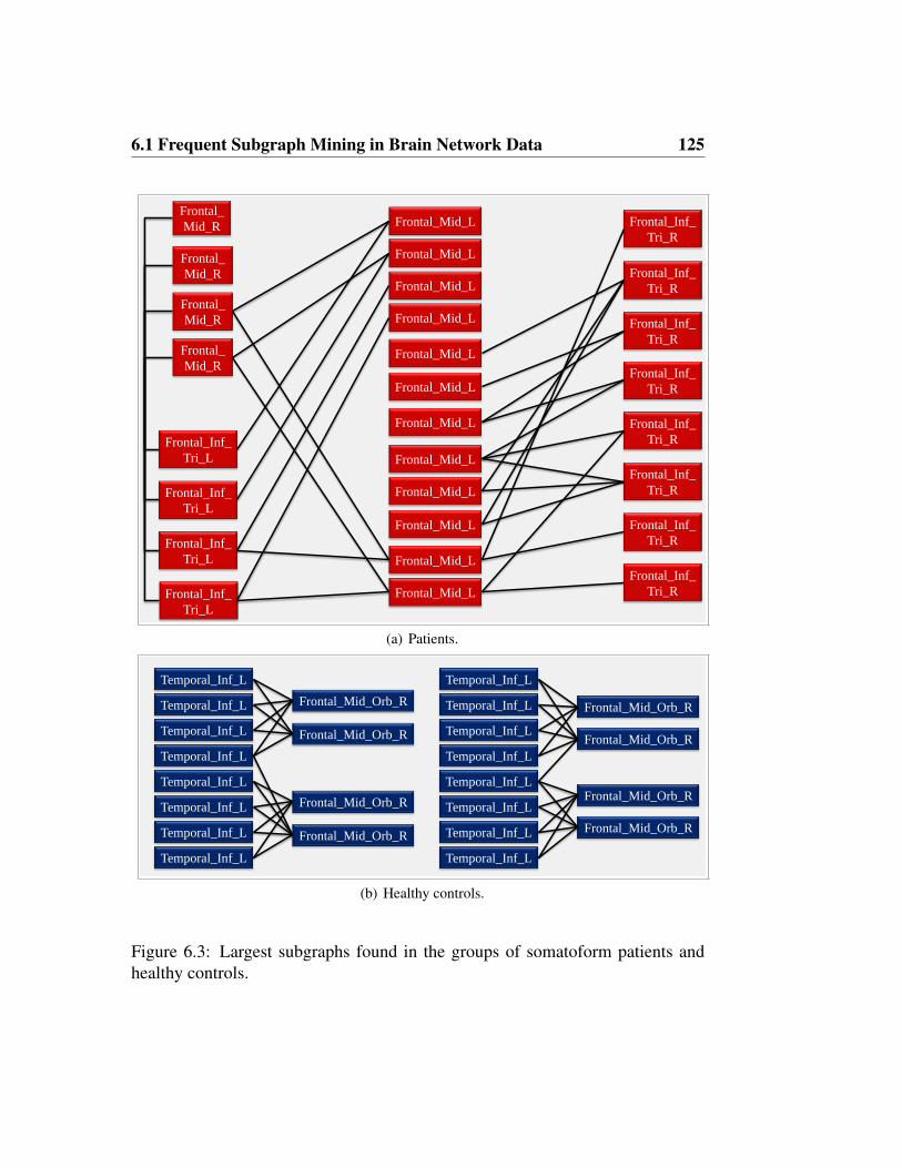
6.1 Frequent Subgraph Mining in Brain Network Data 125
Frontal_Inf_
Tri_R
Frontal_Mid_L
Frontal_Mid_L
Frontal_Mid_L
Frontal_Mid_L
Frontal_Mid_L
Frontal_Mid_L
Frontal_Mid_L
Frontal_Mid_L
Frontal_Mid_L
Frontal_Mid_L
Frontal_Mid_L
Frontal_Mid_L
Frontal_
Mid_R
Frontal_Inf_
Tri_L
Frontal_
Mid_R
Frontal_
Mid_R
Frontal_
Mid_R
Frontal_Inf_
Tri_L
Frontal_Inf_
Tri_L
Frontal_Inf_
Tri_L
Frontal_Inf_
Tri_R
Frontal_Inf_
Tri_R
Frontal_Inf_
Tri_R
Frontal_Inf_
Tri_R
Frontal_Inf_
Tri_R
Frontal_Inf_
Tri_R
Frontal_Inf_
Tri_R
(a) Patients.
Temporal_Inf_L
Temporal_Inf_L
Temporal_Inf_L
Temporal_Inf_L
Temporal_Inf_L
Temporal_Inf_L
Temporal_Inf_L
Temporal_Inf_L
Frontal_Mid_Orb_R
Frontal_Mid_Orb_R
Temporal_Inf_L
Temporal_Inf_L
Temporal_Inf_L
Temporal_Inf_L
Temporal_Inf_L
Temporal_Inf_L
Temporal_Inf_L
Temporal_Inf_L
Frontal_Mid_Orb_R
Frontal_Mid_Orb_R
Frontal_Mid_Orb_R
Frontal_Mid_Orb_R
Frontal_Mid_Orb_R
Frontal_Mid_Orb_R
(b) Healthy controls.
Figure 6.3: Largest subgraphs found in the groups of somatoform patients andhealthy controls.

126 6. Graph Mining
most frequent ROI (freqnorm = 6.43%). The most frequent ROI w.r.t. thesubgraphs of the control group is Frontal Mid Orb R (freqnorm = 22.04%).ROIs that show a small frequency are summarized by the label Miscellaneous.Our results are consistent with a previous study [41]. They report different ac-tivation pattern in the regions Insula L (Patients: freqnorm = 5.29% Controls:freqnorm = 1.95%) and Frontal Mid Orb R (Patients: freqnorm = 3.38% Con-trols: freqnorm = 22.04%), the key-player in the group of healthy controls. Ourresults of different activation of the parahippocampal cortex in patients and con-trols (not depicted in Figure 6.4) supports a recent study that suggests that pa-tients with posttraumatic stress disorder showed also an altered activation patternin the parahippocampal cortex in comparison to healthy controls when subjectedto painful heat stimuli [37]. In addition, we found that patients show increased ac-tivation in Rolandic Oper L, Caudate R and Rectus R whereas the control groupis activated in the regions Temporal Inf L, Heschl R and Lingual R to a higherdegree. Also, the olfactory region shows alterations in the activation of patientsand controls. Whereas Olfactory R occurs to a much higher degree in subgraphsfound in patients, subgraphs found in the networks of controls are labeled moreoften with Olfactory L.
Finding Frequent Subgraphs with FANMOD
The public disposable FANMOD tool2, implementing the exhaustive samplingalgorithm by [102], is restricted to networks with a maximum number of 16 dif-ferent vertex labels. Hence, we map the original network data to a modified ver-sion where only the 15 most frequent ROIs are kept. The remaining vertices arelabeled by Miscellaneous. This labeling scheme refers to the ROI distributionamong subgraphs detected by GREW as shown in Figure 6.4. As edges of thetype Miscellaneous–Miscellaneous occur disproportional frequent within the net-work, and would therefore tamper with the real frequencies of the results, weignored that kind of interaction.
2http://theinf1.informatik.uni-jena.de/motifs/

6.1 Frequent Subgraph Mining in Brain Network Data 127
Caudate_RRectus_RInsula_LOccipital_Mid_LTemporal_Sup_RRolandic_Oper_LFrontal_Sup_Medial_LPutamen_LThalamus_LFrontal_Mid_LFrontal_Mid_Orb_ROlfactory_RRectus_LFrontal_Sup_Orb_R
(a) Patients.
Frontal_Mid_Orb_RTemporal_Inf_LLingual_RParacentral_Lobule_RCalcarine_LPostcentral_ROlfactory_LCaudate_LTemporal_Sup_LFusiform_RPrecuneus_RTemporal_Pole_Sup_RFrontal_Mid_LFrontal_Mid_Orb_L
(b) Healthy controls.
Figure 6.4: Frequencies of ROIs in subgraphs of patients and controls, respec-tively.

128 6. Graph Mining
Table 6.2: Subgraphs detected by FANMOD for different number of vertices com-pared to the number of subgraphs found by GREW, respectively. For some motifsizes, FANMOD is not applicable as the runtime effort for exhaustive enumerationgrows exponentially in the size of the subgraphs.
SUBJECT k = 3 k = 4 k = 5 k = 6 3 ≤ k ≤ 6 # SUBGRAPHS
BY GREWPAT 1 9 13 28 42 92 4PAT 2 42 121 288 - 451 406PAT 3 5 6 7 8 26 4PAT 4 22 91 374 - 487 56PAT 5 139 509 - - 648 988PAT 6 431 3,292 - - 3,723 1,861CONT 1 6 10 16 22 54 34CONT 2 18 32 51 78 179 56CONT 3 9 26 - - 35 161CONT 4 137 565 2,399 - 3,101 472
We searched for subgraphs, consisting of up to six vertices and used a samplerate of 100,000 to estimate the number of subgraphs which is the default param-eterization, as recommended by the authors. Table 6.2 illustrates the number ofsubgraphs that comprise 3 ≤ k ≤ 6 vertices for each subject. We comparedthese results by applying GREW (t = 5) to the same modified networks. Thelast column of Table 6.2 demonstrates that for small subgraph sizes an exhaustivemethod provides significant more information about the graph structure. Notethat the total number of detected subgraphs by FANMOD with a limited numberof vertices exceeds the total number of subgraphs found by GREW with arbitrarysize in most cases. However, an exhaustive method is only applicable for findingsubgraphs that consist of a small number of vertices.

6.1 Frequent Subgraph Mining in Brain Network Data 129
6.1.3 Conclusions
In this work, we have applied GREW, a heuristic approach for finding frequentsubgraphs in one large network and the algorithm FANMOD, an exhaustive sam-pling method for frequent subgraph discovery. We executed both algorithms onunion graph models resulting from time series data of six somatoform patients andfour healthy controls. The detected subgraphs represent groups of brain compart-ments that covary in their activity during the process of pain stimulation. We eval-uated the appearance of subgraphs for both groups. Our results let us suspect thatsomatoform brain disorder is caused by an additional pathogeneous activity, notby a missing physiological activity. So far we care about the topology of the net-work, but ignore the temporal order of these interactions. When studying networktopology, it is important to bear in mind that the network models currently avail-able are simplified models of the systems that govern cellular processes. Whilethese processes are dynamic, the models we consider so far are all static.
In the next Section, we extend this idea to perform real dynamic graph miningon biological yeast network data.

130 6. Graph Mining
6.2 Motif Discovery in Dynamic Yeast Network Data
The majority of recent subgraph mining approaches have focused on character-izing the topology of static networks. But to model real-world systems, often atemporal component has to be taken into account, as interactions between objectshere usually occur for a certain period of time only. Therefore, a realistic modelhas to consider that edges will be inserted and/or deleted over time. The resultingdata structure is called a dynamic graph.
These dynamic graphs occur in many real-world applications. In Biology, awide-spread approach is to model interacting proteins as networks, where eachvertex corresponds to a protein and two vertices are connected by an edge if thecorresponding proteins can bind. In addition, further technologies allow biologiststo measure the distribution of protein interactions at different time points. Hence,associating a time series for each protein provides interesting insights into thedynamically changing system. In social networks like Facebook, people contacteach other at specific time points and form various complex relationships.
Our new approach for frequent subgraph discovery, provided in this section,performs data mining on such dynamic graphs in an on-top fashion, i.e. we searcha set of frequent static subgraphs for frequent dynamic patterns. Existing subgraphmining algorithms on static graphs can be easily integrated into our framework tomake them handle dynamic graphs. The search for dynamic patterns is based onthe idea of suffix trees.
6.2.1 Performing Graph Mining on Dynamic Network Data
Now we provide the essential definitions from dynamic graph theory necessary tofollow our argumentation, based on the definitions of classic graph theory, pre-sented in Section 6.1.1.
Basics of Dynamic Graph Theory
First, we give the formal definition of a time series of graphs.

6.2 Motif Discovery in Dynamic Yeast Network Data 131
a c c d
a
a d
bb
εaε
b bεbacε
εad
cdb
Figure 6.5: Transformation of a time series of graphs into a dynamic graph. Thethree graphs on the left represent a time series of graphs with edge insertionsand edge deletions over time. The graph on the right is a dynamic graph thatsummarizes all information represented by the time series.
Definition 16 (Time Series of Graphs) Given a sequenceGts of n graphs {G1, . . . ,
Gn} with Gi = (Vi, Ei, Li, li) for 1 ≤ i ≤ n. We define Gts to be a time seriesof graphs if V1 = Vi for all 1 ≤ i ≤ n. Gi is the i-th state of Gts and Ai is the
adjacency matrix of the i-th state. In every state i, li : Vi∪Ei → Li assigns labels
to nodes and edges.
Note that li is not necessarily the same for all 1 ≤ i ≤ n. This means that anedge (or even a node) might change its label in consecutive time steps of the timeseries. Such a time series of graphs can be transformed into a dynamic graph asfollows:
Definition 17 (Dynamic Graph) Given a time series of graphs Gts of n graphs.
Then the dynamic graphDG(Gts) ofGts is defined asDG(Gts) = (VDG, EDG, `),
where VDG = Vi for all 1 ≤ i ≤ n and EDG = ∪ni=1Ei. The mapping ` : EDG →L ∪ ε maps each edge e in EDG to a string `(e) of length n, referred to as the
edge existence string of e. Let us denote the i-th character of `(e) as `(e(i)).
`(e(i)) = ε if e does not exist in state i of Gts. If e does exist in state i of Gts, then
`(e(i)) = li(e).
Hence, a dynamic graph is a union graph (cf. Definition 15) over a time series ofgraphs in combination with the corresponding existence string. An example forsuch a transformation is depicted in Figure 6.5.

132 6. Graph Mining
To extend frequent subgraph discovery to dynamic networks, we have to definetwo types of frequent subgraphs:
Definition 18 (Static Frequent Subgraph) A subgraph GSts that has more than
t embeddings in a dynamic graph DG(Gts) is called a static frequent subgraph.
In other terms, static frequent subgraphs in a dynamic graph are subgraphs that aretopologically frequent in the summary graph. Hence, edge existence strings playno role when looking for static frequent subgraphs. The static frequent subgraphsin a dynamic graph are defined in exactly the same manner as frequent subgraphson one single network. A dynamic pattern D is a static frequent subgraph S
such that in more than u embeddings of S, edge insertions, deletions and labelchanges occur in the same temporal order. As we want to study cases where theseinsertions and deletions happen in a subsection of the complete time series only,we now have to make use of the existence strings of the edges.
Definition 19 (Common Substring) For two strings s1 and s2 of length |s1| and
|s2|, sub(s1, i, j) = sub(s2, i, j) means that the substrings from the i-th to the j-th
character in s1 and s2 are identical, where 1 ≤ i ≤ j ≤ min(|s1|, |s2|). This
identical substring is called a common substring of s1 and s2.
Definition 20 (Common Dynamic Pattern) Let S be a static frequent subgraph
in dynamic graph DG, and let S1 = (VS1 , ES1) and S2 = (VS2 , ES2) be two
embeddings of S in DG. As S1 and S2 are isomorphic, there must be a bijection
f between ES1 and ES2 . Then S1 and S2 share a common dynamic pattern from
position i to j if for all pairs of edges (e1, e2) from ES1 × ES2 where e2 = f(e1)
the following equality holds: sub(`(e1), i, j) = sub(`(e2), i, j), i.e. the existence
strings of corresponding edges are identical from position i to position j.
If enough embeddings of the same static frequent subgraph share the same com-mon dynamic pattern, then this static frequent subgraph contains a dynamic fre-quent subgraph. Note, that common dynamic patterns consider edge labels, whereasstatic frequent subgraphs ignore the labeling.

6.2 Motif Discovery in Dynamic Yeast Network Data 133
Definition 21 (Dynamic Frequent Subgraph) Let S be a static frequent sub-
graph with u embeddings {S1, . . . , Su} in a dynamic graph DG. Let t be a user-
defined frequency threshold. If at least t embeddings of S share the same common
dynamic pattern, then the topology of S and the common dynamic pattern repre-
sent a dynamic frequent subgraph.
For instance, in our real-world case study presented in this section, a dynamicfrequent subgraph describes a set of groups of proteins that show similar patternsof co-expression during a certain interval of a time series.
Dynamic Graph Mining
After defining frequent subgraphs in dynamic networks, we now present an effi-cient algorithmic solution on how to compute them. Our framework is based onthe idea of suffix trees. Dynamic frequent subgraph discovery can be performedin an on-top fashion in two steps. First, we employ one of the state-of-the-artalgorithms for finding frequent subgraphs in the union graph of a time series ofgraphs (cf. Section 2.4). Second, we search the resulting static frequent subgraphsfor frequent dynamic patterns. Figure 6.6 visualizes an example for frequent sub-graph discovery in a dynamic network.
Matrix Representation of Embeddings. To discover dynamic patterns we pro-cess the results of a static frequent subgraph mining algorithm (see Figure 6.6(a)).Key to our efficient scheme is to represent each embedding of a frequent staticsubgraph by the set of existence strings of its edges. Hence, for each of the sembeddings of a static frequent subgraph S with m edges, we obtain a set of mexistence strings. We represent these sets of strings for one embedding Si of Sas an m × n matrix, M(Si), where each row corresponds to one edge, and eachcolumn to one time point in the time series (see Figure 6.6(b)).
Canonical Edge Order. To compare the matrices M(S1) and M(S2) of twodifferent embeddings S1 and S2 of the same subgraph S efficiently, we have to

134 6. Graph Mining
bac
εac
ccε cεb
εcε aεb
(a) TwoEmbeddings.
edge ε a c
edge c ε b
edge c c ε
concatenation <1:εcc> <2:aεc> <3:cbε>
edge b a c
edge a ε b
edge ε c ε
concatenation <1:baε> <2:aεc> <3:cbε>
time point 1 2 3
(b) Matrix representation.
edge ε a c
edge c ε b
edge c c ε
concatenation <1:εcc> <2:aεc> <3:cbε>
edge b a c
edge a ε b
edge ε c ε
concatenation <1:baε> <2:aεc> <3:cbε>
time point 1 2 3
(c) Common substring.
cε
ac
εb
(d) Dynamic pattern.
Figure 6.6: Two embeddings (6.6(a)) of the same static frequent subgraph andtheir common dynamic pattern depicted as dynamic graph (6.6(d)). The two em-beddings are shown with their matrix and string representation each (6.6(b)). Intime step 2 and 3, edge insertions and deletions occur simultaneously in both em-beddings. This is the common substring (6.6(c)) that refers to the dynamic pattern.

6.2 Motif Discovery in Dynamic Yeast Network Data 135
define a canonical ordering of edges for all embeddings of S. gSpan [107] ordersthe edges in each embedding of a frequent subgraph according to a Depth FirstSearch on the vertices (cf. Section 2.4.1). In this manner, we can sort the rows ofall matrices representing embeddings of the same subgraph such that correspond-ing edges are represented by the same row in each of these matrices.
String Representation of Embeddings. Using this canonical form of the ma-trices dynamic frequent subgraph discovery is equivalent to detecting identicalblocks of columns. Therefore we transform each matrix into a string representa-tion by treating each column in the matrix as one symbol which is just the con-catenation of all entries in this column. We obtain s strings, each describing oneembedding, which have a common substring if the embeddings show identicaldynamic behavior over a certain period of time (see Figure 6.6(c)).
Frequent Common Substring Discovery. A classic result from the field ofstring algorithms [50] helps us to discover these common substrings extremelyefficiently: detecting all longest substrings in a set of s strings is possible in linearruntime, by reading all strings exactly once by employing a suffix tree to store allsubstrings from a set of strings. A simple breadth-first search in the tree then pro-vides all frequent common substrings. Obviously, each of these frequent commonsubstrings corresponds to one dynamic pattern (see Figure 6.6(d)). To guaranteethat all embeddings of a dynamic pattern start at the same time point of the timeseries, we include a time stamp into our matrix representation of each embedding,by adding an extra row to the matrix, which numbers the time steps from 1 to n,where n is the number of time steps in the time series. We then include these timestamps into the string representation of our matrix.
136 6. Graph Mining
6.2.2 Dynamic Network Construction
In this section, we confirm the practical feasibility of our framework for findingfrequent subgraphs in dynamic networks on the basis of a large case study onreal-world biological data. We describe in detail how to construct the dynamicnetwork models by a combination of interaction data and a time series dataset.
Protein-Protein-Interaction Datasets. We created a dynamic network by inte-grating protein-protein-interaction (PPI) data from yeast and a time series of yeastgene expression levels. We obtained the yeast PPI network data from the databaseDIP (Database of Interacting Proteins) [106, released on January 6, 2008], con-taining all pairs of interacting proteins identified in the yeast organism S. cere-
visiae. This dataset consists of 4,923 proteins, which are the original set of nodesin our dynamic graph and 18,324 interactions representing edges between thenodes.
Vertex Labels. In order to assign labels to all nodes of the network, we mappedthe proteins to their corresponding protein-coding open reading frames (ORFs),via information provided by the SGD (Saccharomyces Genome Database) [46]from DIP. Finally, we determined the ‘molecular function’ associated with thisORF in the Gene Ontology (GO) hierarchy at depth two [5]. As GO terms are or-ganized in directed acyclic graphs, and each term can be traced to different depths,it can occur that multiple GO annotations can be assigned to one single ORF at agiven depth. As current methods for frequent subgraph mining and enumerationrequire a unique label, we retained all ORFs with a non-ambiguous GO labelingat depth two. The twelve remaining GO functional classes were then used as nodelabels for the remaining proteins.
Time Series Datasets. Next we used a cell cycle time series of yeast gene ex-pression levels by [22], available from the ExpressDB collection of yeast RNAExpression Datasets [2]. The dataset consists of 6,601 time series of 17 measure-

6.2 Motif Discovery in Dynamic Yeast Network Data 137
ments for 6,259 ORFs, of which 6,045 ORFs can be mapped to one unique timeseries. 3,607 ORFS are both present in our GO-labeled yeast PPI network and inthe gene expression dataset. The corresponding proteins are the final set of nodesin our dynamic graph, other nodes and their adjacent edges from the original graphwere skipped. The final network comprises 3,607 nodes, twelve different classesof node labels, 7,395 edges per time step, and 17 time steps.
Edge Existence Strings. Each edge in our dynamic network was assigned anedge existence string (cf. Definition 17) of length 17 according to the followingrules: We distinguish three basic categories of gene expression levels for eachgene g at each time point i. We refer to its expression level at time point i as g(i).Categories are assigned by comparing the median expression level of g across thetime series with the z–scoremedian of g(i):
z–scoremedian(g(i)) =g(i)−medianj∈{1,..,n}g(j)√
1n
∑(g(k)−medianj∈{1,..,n}g(j))2
This results in three different expression levels:
• High:g(i) is significantly higher than the median expression level of g, i.e.z–scoremedian(g(i)) ≥ 2. That indicates that g supports important steps ofthe examined biological process, or regulates small subunits.
• Medium:g(i) does not significantly differ from the median expression level of g, i.e.-2< z–scoremedian(g(i))< 2. That means that g does not play an importantrole in the examined biological process.
• Low:g(i) is significantly lower than the median expression level of g, i.e.z–scoremedian(g(i)) ≤ -2. That argues for a repression functionality of g inthe examined biological process.

138 6. Graph Mining
For each edge e in our dynamic graph, we compared the expression profiles ofits adjacent genes g1 and g2 to generate the edge existence string according to thefollowing rules:
• `(e(i)) = ’H’ if g1(i) and g2(i) both show a high gene expression level.
• `(e(i)) = ’M’ if g1(i) and g2(i) both show a medium gene expression level.
• `(e(i)) = ’L’ if g1(i) and g2(i) both show a low gene expression level.
For pairs of genes g1 and g2 that show different gene expresson levels, we addi-tionally introduce the character ’N’. In this manner, we generated edge existencestrings from the alphabet Σ = {H,L, M,N} for pairs of interacting genes in theyeast PPI network.
Enumerating all Static Frequent Subgraphs
In order to compute exact frequencies for static frequent sugraphs, we exhaus-tively enumerated all frequent subgraphs of our dynamic network. This step wasperformed using the FANMOD tool3. As our dynamic network is a large graph,we have to limit ourselves to subgraphs covering three or four vertices as previ-ous studies [105], but this allows us to guarantee that we are not missing out ondynamic frequent subgraphs.
3http://theinf1.informatik.uni-jena.de/motifs/

6.2 Motif Discovery in Dynamic Yeast Network Data 139
6.2.3 Evaluation of Dynamic Frequent Subgraphs
Now we describe how to evaluate the detected motifs according significance andthe evolutionary conservation rate among different species.
Significance of Dynamic Frequent Subgraphs
To assess the significance of a static frequent subgraph with frequency t, we usep-values for each static frequent subgraph according to [102]. The p-value repre-sents the probability of this static frequent subgraph occurring at least t times ina random graph with identical degree distribution. We only retain those static fre-quent subgraphs whose p-value is below the significance level of α = 0.025. Wealso assess the significance of the common dynamic string pattern σ of a dynamicfrequent subgraph D which occurs in u out of t embeddings of the static frequentsubgraph S in terms of a p-value. For this purpose, we compute the probabilityp of σ to occur in an embedding of S by chance. Let M = M(i, j)l′×n′ be thematrix representation of σ, where each row corresponds to one edge (existencestring) and each column to one time step. We then define the probability of σoccurring by chance as
pσ =l′∏i=1
n′∏j=1
pi(M(i, j)),
where pi is the background probability of the character represented by M(i, j)
occurring in the i-th edge of S. In other terms, the random model assumes thatthe existence strings of the embeddings of S were randomly generated. Underthis model, the probability of σ appearing u times (denoted |σ| = u) in the tembeddings of S then follows a binomial distribution:
P (|σ| = u) =
(t
u
)puσ(1− pσ)t−u,
and the p-value of the common dynamic pattern σ can be computed straightfor-wardly:

140 6. Graph Mining
p-value(|σ| = u) = P (|σ| ≥ u)
We deem common dynamic patterns significant, if their p-value is below 0.025.Dynamic frequent subgraphs are considered significant if their associated staticfrequent subgraph is significant and if its common dynamic pattern is significantas well. We only retained those dynamic frequent subgraphs that occur in at least50% of the embeddings of the corresponding static frequent subgraph.
Evolutionary Conservation Rate: A Quality Criterion for Dynamic FrequentSubgraphs
The evolutionary conservation rate is known to be a good quality criterion inbiology. Following previous biological analysis [89], we deem dynamic fre-quent subgraphs the more conserved, the more proteins that participate in embed-dings of this subgraph have identifiable orthologs in other organisms. We analysethe conservation rate of yeast proteins by searching for orthologs (i.e. homolo-gous sequences that were separated by a speciation event) in each of five otherhigher eukaryotic organisms for which information is available in the InParanoiddatabase [84]: 644 of the 3,607 proteins in our dynamic network turned out tobe conserved across all five species. Hence the probability of observing a con-served protein by uniform random sampling from the PPI network is 0.1785, ofobserving a set of three conserved proteins is 0.0057, and of observing a set offour conserved proteins is 0.0010.
Conservation Rate among Static and Dynamic Frequent Subgraphs
Our static frequent subgraph discovery results in 367 subgraphs with three nodesand within these 515 dynamic patterns that were both frequent and significant. Wefound 2,302 proteins to be members of at least one static frequent subgraph, out ofwhich 577 are conserved across species (conservation rate 0.2507). Hence the rateof conservation among proteins that are part of static frequent subgraphs is signif-

6.2 Motif Discovery in Dynamic Yeast Network Data 141
icantly higher than among proteins that are sampled randomly from our dynamicnetwork (Binomial distribution B(t = 2, 302; p = 0.1785); p-value < 0.0001).1,787 proteins are members of at least one dynamic frequent subgraph, including477 conserved proteins (conservation rate 0.2669). Hence the rate of conserva-tion among proteins that are part of dynamic patterns is significantly higher thanamong proteins that are sampled randomly from our dynamic network (Binomialdistribution B(t = 1, 787; p = 0.1785); p-value < 0.0001). 515 proteins aremembers of at least one static frequent subgraph, but of none of the dynamic pat-terns (100 of these are conserved, conservation rate 0.1942). While the rates ofconservation among proteins from static and dynamic frequent subgraphs are notsignificantly different (two-sample t-test for unequal variances, p = 0.2392), weobserved that proteins that participate in static and dynamic frequent subgraphsare significantly stronger conserved than those that are members of static, but not
of dynamic static subgraphs (two-sample t-test for unequal variances, p = 0.004).
Table 6.3: Evaluation w.r.t. conservation rate of static and dynamic frequent sub-graphs with three and four nodes.
k = 3 k = 4
STAT. DYN. STAT. STAT. DYN. STAT.ONLY ONLY
# FREQUENT
SUBGRAPHS 367 515 3,293 2,111
# PROTEINS 2,302 1,787 515 2,403 1,770 633# CONSERVED
PROTEINS 577 477 100 591 470 121CONSERVATION
RATE 0.2507 0.2669 0.1942 0.2459 0.2655 0.1912
We discovered 3,293 static frequent subgraphs of size k = 4. Within thesesubgraphs we found 2,111 dynamic patterns that were both frequent and signifi-cant. 2,403 proteins are members of at least one static frequent subgraph, out of
142 6. Graph Mining
which 591 are conserved (conservation rate 0.2459). Consistent with our resultson frequent subgraphs with three nodes the rate of conservation among proteinsthat are part of static frequent subgraphs is significantly higher than among pro-teins that are sampled randomly from our dynamic network (Binomial distributionB(t = 2, 403; p = 0.1785); p-value < 0.0001). 1,770 proteins are members ofat least one dynamic pattern, including 470 conserved proteins (conservation rate0.2655). Analogously to the frequent subgraphs with three nodes the rate of con-servation among proteins that are part of dynamic patterns is significantly higherthan among proteins that are sampled randomly from our dynamic network (Bi-nomial distribution B(t = 1, 770; p = 0.1785); p-value < 0.0001). 633 proteinsare members of at least one static frequent subgraph, but of none of the dynamicpatterns (121 of these are conserved, conservation rate 0.1912). While the ratesof conservation among proteins from static and dynamic frequent subgraphs withfour nodes are not significantly different (two-sample t-test for unequal variances,p = 0.1525), we observed that proteins that participate in static and dynamicfrequent subgraphs are significantly stronger conserved than those that are mem-bers of static, but not of dynamic ones (two-sample t-test for unequal variances,p = 0.001). Therefore the significance of the conservation rate of frequent sub-graphs with four nodes is even higher than for subgraphs with three nodes. Ta-ble 6.3 summarizes the results of these experiments.
Conservation of Dynamic Frequent Subgraphs across GO Classes
We also checked whether proteins that are part of static and dynamic subgraphsshow different levels of conservation depending on their molecular function asdefined by GO. As can be seen from Figure 6.7, conservation rates vary widelyamong different functional classes, both for background conservation rate, andamong dynamic and static frequent subgraphs. The figure shows the conserva-tion rates for proteins that are participating in frequent subgraphs with three andfour nodes w.r.t. twelve different classes of protein functions. For each func-tion the general conservation rate of proteins among this class is depicted. The

6.2 Motif Discovery in Dynamic Yeast Network Data 143
20
30
40
50
tion
rate
(%) all proteins
proteins in static motifsproteins in static and dynamic motifsproteins in static but not dynamic motifs
0
10
cons
erva
t
(a) k = 3.
10
20
30
tion
rate
(%) all proteins
proteins in static motifsproteins in static and dynamic motifsproteins in static but not dynamic motifs
0
10
cons
erva
t
(b) k = 4.
Figure 6.7: Evaluation w.r.t. protein function of frequent subgraphs with three andfour nodes.
second, third and fourth bars of the histogram stand for the conservation rate ofproteins involved in static frequent subgraphs, in dynamic patterns (therefore alsoin static frequent subgraphs) and the conservation rate of proteins that play a rolein static frequent subgraphs only. It can be seen that frequent subgraphs with threeand four nodes both show differences in their conservation rate depending on theprotein functions. For example, proteins with structural molecule activity or pro-teins regulating transcription participating only in static frequent subgraphs arehighly conserved in subgraphs with three nodes exclusively. Proteins that havemetallochaperone activity or regulate translation or chaperones are not conserved,neither in static nor in dynamic patterns.
Selected Frequent Subgraphs
The most frequent and significant (p < 0.0001) subgraph with three nodes (cf.Figure 6.8(a)) has 4,060 embeddings. Two proteins share the same biologicalfunction catalytic activity, whereas the third is a transporter protein. Transporterproteins catalyze the transfer of a substance from one side of a membrane to theother. Within these 4,060 embeddings we detect 1,728 dynamic patterns com-prising two time points. Figure 6.8(b) shows a significant (p < 0.0001) subgraph

144 6. Graph Mining
Catalytic Activity
Catalytic Activity
Transporter Activity
M M
M M
(a) Highest number of embeddings (k = 3).
Motor Activity
Enzyme Regulator
Activity
Binding
M M M M N N M M N M M M M M M N
M M M M M M M M N M M M M M M N
(b) Longest dynamic pattern (k = 3).
Binding
Binding
Catalytic Activity
M M
M MCatalytic Activity
M M
(c) Highest number of embeddings (k = 4).
Binding
Transporter Activity
N M M ...
Transcription
Regulator Activity
Activity
Enzyme Regulator
ActivityL M M ...
N M M ...
L M M M ...
(d) Longest dynamic pattern (k = 4).
Figure 6.8: Selected frequent subgraphs that consist of three or four nodes.
with three embeddings, but in two of them we detect a dynamic pattern that hasidentical behavior of co-expression over a period of 16 out of 17 time points. Thecorresponding interacting proteins are organized under binding, enzyme regulator
activity and motor activity term of GO, respectively. This static frequent subgraphhas quite few embeddings, but includes the longest dynamic pattern within staticfrequent subgraphs of size k = 3.
The most frequent subgraph of size k = 4 has 18,056 embeddings, illustratedin Figure 6.8(c). Two proteins show catalysis properties whereas the other two arebinding proteins. 8,511 out of these embeddings have dynamic patterns compris-ing two time points. In Figure 6.8(d) the most significant (p < 0.0001) subgraphhas three embeddings, whereof two have a dynamic pattern over a time period of

6.2 Motif Discovery in Dynamic Yeast Network Data 145
15 time steps. In the first time step both the binding protein and the transportationprotein show very low expression levels.
6.2.4 Conclusions
We have presented a framework for frequent dynamic subgraph discovery in dy-namic graphs. We have shown how to efficiently compute these patterns usingsuffix trees. Furthermore, we have described how to combine frequent subgraphmining algorithms with our dynamic framework and we have applied our frame-work on a large real-world case study to handle dynamic graphs. Dynamic graphmining is a technique that can be used in many fields of applications. Finding dy-namic patterns in PPI maps promises to reveal interesting insights into biologicalprocesses.

146 6. Graph Mining

Chapter 7
Data Mining Using GraphicsProcessors
In recent years, Graphics Processing Units (GPUs) have evolved from simpledevices for the display signal preparation into powerful coprocessors supportingthe CPU in various ways. Graphics applications such as realistic 3D games arecomputationally demanding and require a large number of complex algebraic op-erations for each update of the display image. Therefore, today’s graphics hard-ware contains a large number of programmable processors which are optimizedto cope with this high workload of vector, matrix, and symbolic computations ina highly parallel way. In terms of peak performance, the graphics hardware hasoutperformed state-of-the-art multi-core CPUs by a large margin.
We focus on exploiting the computational power of GPUs for data mining. Ithas been shown that many data mining algorithms, including clustering can besupported by a powerful database primitive: The similarity join [9]. This oper-ator yields as result all pairs of objects in the database having a distance of lessthan some predefined threshold εSJ . To show that also the more complex basicoperations of similarity search and data mining can be supported by novel parallelalgorithms specially designed for the GPU, we present in Section 7.3 two algo-rithms for the similarity join, one being a nested block loop join, and one being an
148 7. Data Mining Using Graphics Processors
indexed loop join. Therefor specialized indexing methods are required because ofthe highly parallel but restricted programming environment (cf. Section 7.1). InSection 7.2, we propose such an indexing method.
Finally, to demonstrate that highly complex data mining tasks can be effi-ciently implemented using novel parallel algorithms, we propose parallel versionsof two widespread clustering algorithms in Sections 7.4 and 7.5. The first algo-rithm CUDA-DClust combines the high computational power and the multiple ad-vantages provided by the density-based clustering algorithm DBSCAN [31]. Thisapproach is highly parallel and exploits thus the high number of simple SIMD(Single Instruction Multiple Data) processors of today’s graphics hardware. Theparallelization which is required for GPUs differs considerably from previousparallel algorithms which have focused on shared-nothing parallel architecturesprevalent in server farms. For even further acceleration, we also propose the al-gorithm CUDA-DClust*, the indexed variant of CUDA-DClust. In addition, weintroduce a parallel version of k-means clustering [72] which follows an algorith-mic paradigm that is very different from density-based clustering. We demonstratethe superiority of our approaches over the corresponding sequential algorithms onCPU.
All algorithms for the GPU have been implemented using NVIDIA’s tech-nology Compute Unified Device Architecture (CUDA) [1]. Vendors of graphicshardware have recently anticipated the trend towards general purpose computingon GPU and developed libraries, pre-compilers and application programming in-terfaces to support GP-GPU applications. CUDA offers a programming interfacefor the C programming language in which both the host program as well as thekernel functions are assembled in a single program [1]. The host program is themain program, executed on the CPU. In contrast, the so-called kernel functions
are executed in a massively parallel fashion on the (hundreds of) processors inthe GPU. An analogous technique is also offered by ATI using the brand namesClose-to-Metal, Stream SDK, and Brook-GP.

7.1 The GPU Architecture 149
Figure 7.1: Architecture of a GPU.
7.1 The GPU Architecture
From the hardware perspective, a GPU consists of a number of multiprocessors,each of which consists of a set of simple processors which operate in a SIMDfashion, i.e. all processors of one multiprocessor execute in a synchronized waythe same arithmetic or logic operation at the same time, potentially operating ondifferent data. For instance, a GPU of the newest generation GT200 (e.g. on thegraphics card GeForce GTX280) has 30 multiprocessors, each consisting of eightSIMD-processors, summarizing to a total amount of 240 processors inside oneGPU. The computational power sums up to a peak performance of 933 GFLOP/s.
7.1.1 The Memory Model
Apart from some memory units with special purpose in the context of graphicsprocessing (e.g. texture memory), we have three important types of memory, asvisualized in Figure 7.1. The shared memory (SM) is a memory unit with fastaccess (at the speed of register access, i.e. no delay). The shared memory isshared among all processors of a multiprocessor. It can be used for local variablesbut also to exchange information between threads on different processors of thesame multiprocessor. It cannot be used for information which is shared amongthreads on different multiprocessors. The shared memory is fast but very limitedin capacity (16 KBytes per multiprocessor).

150 7. Data Mining Using Graphics Processors
The second kind of memory is the so-called device memory (DM), which is the ac-tual video RAM of the graphics card (also used for frame buffers etc.). The devicememory is physically located on the graphics card (but not inside the GPU), is sig-nificantly larger than shared memory (typically up to some hundreds of MBytes),but also significantly slower. In particular, memory accesses to device memorycause a typical latency delay of 400-600 clock cycles (on G200-GPU, correspond-ing to 300-500ns). The bandwidth for transferring data between device memoryand GPU (141.7 GB/s on G200) is higher than that of CPU and main memory(about 10 GB/s on current CPUs). The device memory can be used to share in-formation between threads on different multiprocessors. If some threads schedulememory accesses from contiguous addresses, these accesses can be coalesced,i.e. taken together to improve the access speed. A typical cooperation patternfor device memory and shared memory is to copy the required information fromdevice memory to shared memory simultaneously from different threads (if pos-sible, considering coalesced accesses), then to let each thread compute the resulton shared memory, and finally, to copy the result back to device memory.
The third kind of memory considered here is the main memory which is notpart of the graphics card. The GPU has no access to the address space of the CPU.The CPU can only write to or read from device memory using specialized APIfunctions. In this case, the data packets have to be transferred via the Front SideBus and the PCI-Express Bus. The bandwidth of these bus systems is strictlylimited, and therefore, these special transfer operations are considerably moreexpensive than direct accesses of the GPU to device memory or direct accessesof the CPU to main memory.
7.1.2 The Programming Model
The basis of the programming model of GPUs are lightweight processes which areeasy to create and to synchronize, called threads. In contrast to CPU processes,the generation and termination of GPU threads as well as context switches be-tween different threads do not cause any considerable overhead either. In typical

7.1 The GPU Architecture 151
applications, thousands or even millions of threads are created, for instance onethread per pixel in gaming applications. It is recommended to create much morethreads than the number of available SIMD-processors because context switchesare also used to hide the latency delay of memory accesses: Particularly an accessto the device memory may cause a latency delay of 400-600 clock cycles, andduring that time, a multiprocessor may continue its work with other threads.
The CUDA programming library [1] contains API functions to create a largenumber of threads on GPU, each of which executes a function called kernel func-
tion. These functions (executed in parallel on the GPU) as well as the host pro-
gram (executed sequentially on the CPU) are defined in an extended syntax ofthe C programming language. The kernel functions are restricted in functionality(e.g. no recursion). On GPUs the threads do not even have an individual instruc-tion pointer, but this is rather shared by several threads. For this purpose, threadsare grouped into so-called warps (typically 32 threads per warp). One warp is pro-cessed simultaneously on the eight processors of a single multiprocessor (SIMD)using 4-fold pipelining (totalling in 32 threads executed fully synchronously). Ifnot all threads in a warp follow the same execution path, they are executed in aserialized way. The number of SIMD-processors per multiprocessor as well asthe concept of 4-fold pipelining is constant on all current CUDA-capable GPUs.Multiple warps are grouped into thread groups (TG). It is recommended [1] to usemultiples of 64 threads per thread group. The different warps in a thread group(as well as different warps of different thread groups) are executed independently.The threads in one thread group use the same shared memory and may thus com-municate and share data via the shared memory. The threads in one group can besynchronized, i.e. all threads wait until all warps of the same group have reachedthat point of execution. The latency delay of the device memory can be hidden byscheduling other warps of the same or a different thread group whenever one warpwaits for an access to device memory. To allow switching between warps of dif-ferent thread groups on a multiprocessor, it is recommended that each thread usesonly a small fraction of the shared memory and registers of the multiprocessor [1].

152 7. Data Mining Using Graphics Processors
7.1.3 Atomic Operations
In order to synchronize parallel processes and to ensure the correctness of parallelalgorithms, CUDA offers atomic operations such as increment, decrement, or ex-change (to name just those out of the large collection, which will be needed by ouralgorithms). Most of the atomic operations work on integer data types in devicememory. However, the latest CUDA versions even allow atomic operations inshared memory. If, for instance, some parallel processes share a list as a commonresource with concurrent reading and writing from/to the list, it may be necessaryto (atomically) increment a counter for the number of list entries (which is in mostcases also used as the pointer to the first free list element). Here, atomicity impliesthe following two requirements:
If two or more threads increment the list counter, then (1) the value counterafter all concurrent increments must be equivalent to the value before plus thenumber of concurrent increment operations. And, (2), each of the concurrentthreads must obtain a separate result of the increment operation which indicatesthe index of the empty list element to which the thread can write its information.Hence, most atomic operations return a result after their execution.
For instance, the operation atomicInc has two parameters, the address ofthe counter to be incremented, and an optional threshold value which must not beexceeded by the operation. The operation works as follows: The counter value atthe address is read, and incremented (provided that the threshold is not exceeded).The operation atomicDec works in the inverse way. It also commands two pa-rameters, the address of the counter to be decremented, and an threshold valuethat must not be went below. atomicDec reads the counter value at the address,and decrements that value if it is unequal to zero and larger than the given thresh-old. Finally, the old value of the counter (before incrementing/decrementing) isreturned to the kernel method which invoked atomicInc/atomicDec. If twoor more threads (of the same or different thread groups) call some atomic oper-ations simultaneously, their result is that of an arbitrary sequentialization of theconcurrent operations.

7.2 An Index Structure for the GPU 153
The operation atomicCas works in an analogous way. It performs a Compare-and-Swap operation. It has three parameters, an address, a compare value and aswap value. If the value at the address equals the compare value, the value at theaddress is replaced by the swap value. In every case, the old value at the address(before swapping) is returned to the invoking kernel method.
7.2 An Index Structure for the GPU
Many data mining algorithms for problems like classification, regression, cluster-ing, and outlier detection use similarity queries as a building block. In many cases,these similarity queries even represent the largest part of the computational effortof the data mining tasks. Hence, efficiency is of high importance here. Similarityqueries are defined as follows: Given is a database DS = {x1, · · ·xn} ⊆ Rd of anumber n of vectors from a d-dimensional space, and a query object q ∈ Rd. Wedistinguish between two different kinds of similarity queries, the range queriesand the nearest neighbor-queries:
Definition 22 (Range Query) Let εSJ ∈ R+0 be a threshold value. The result of
the range query is the set of the following objects:
NεSJ (q) = {x ∈ DS : ||x− q|| ≤ εSJ},
where ||x−q|| is an arbitrary distance function between two feature vectors x and
q, e.g. the Euclidean distance.
Definition 23 (Nearest Neighbor Query) The result of a nearest neighbor queryis the set:
NN(q) = {x ∈ DS : ∀x′ ∈ DS : ||x− q|| ≤ ||x′ − q||}.
Definition 23 can also be generalized for the case of the k-nearest neighbor query(NNk(q)), where a number k of nearest neighbors of the query object q is re-

154 7. Data Mining Using Graphics Processors
Points
Figure 7.2: Index structure for GPU.
trieved.
The performance of similarity queries can be significantly improved if a multi-dimensional index structure supports the similarity search. Our index structureneeds to be traversed in parallel for many search objects using the kernel function.Since kernel functions do not allow any recursion, and as they need to have smallstorage overhead by local variables etc., the index structure must be kept very sim-ple as well. To achieve a good compromise between simplicity and selectivity ofthe index, we propose a data partitioning method with a constant number of direc-tory levels. The first level partitions the dataset DS according to the first dimen-sion of the data space, the second level according to the second dimension, andso on. Therefore, before starting the actual data mining method, some transfor-mation technique should be applied which guarantees a high selectivity in the firstdimensions (e.g. Principal Component Analysis, Fast Fourier Transform, DiscreteWavelet Transform, etc.). Figure 7.2 shows a simple, 2-dimensional example ofa 2-level directory (plus the root node which is considered as level-0), similar to[57, 66]. The fanout of each node is eight. In our experiments in Sections 7.3.3and 7.4.3, we used a 3-level directory with fanout 16.
Before starting the actual data mining task, our simple index structure mustbe constructed in a bottom-up way by fractionated sorting of the data: First, thedataset is sorted according to the first dimension, and partitioned into the specified
7.3 Performing the Similarity Join Algorithm on GPU 155
number of quantile partitions. Then, each of the partitions is sorted individuallyaccording to the second dimension, and so on. The boundaries are stored usingsimple arrays which can be easily accessed in the subsequent kernel functions. Inprinciple, this index construction can already be done on GPU, because efficientsorting methods for GPU have been proposed [38]. Since bottom up index con-struction is typically not very costly compared to the data mining algorithm, ourmethod performs this preprocessing step on CPU.
When transferring the dataset from the main memory into the device memory inthe initialization step of the data mining method, our new method has addition-ally to transfer the directory (i.e. the arrays in which the coordinates of the pageboundaries are stored). Compared to the complete dataset, the directory is alwayssmall.
The most important change in the kernel functions in our data mining methodsregards the determination of the εSJ -neighborhood of some given seed object q,which is done by exploiting SIMD-parallelism inside a multiprocessor. In thenon-indexed version, this is done by a set of threads (inside a thread group) eachof which iterates over a different part of the (complete) dataset. In the indexedversion, one of the threads iterates in a set of nested loops (one loop for each levelof the directory) over those nodes of the index structure which represent regionsof the data space which are intersected by the neighborhood-sphere of NεSJ (q).In the innermost loop, we have one set of points (corresponding to a data page ofthe index structure) which is processed by exploiting the SIMD-parallelism, likein the non-indexed version.
7.3 Performing the Similarity Join Algorithm on GPU
The similarity join is a basic operation of a database system designed for sim-ilarity search and data mining on feature vectors. In such applications, we aregiven a database DS of objects which are associated with a vector from a multi-dimensional space, the feature space. The similarity join determines pairs of ob-jects which are similar to each other. The most widespread form is the εSJ -join
156 7. Data Mining Using Graphics Processors
which determines those pairs from DS ×DS which have a Euclidean distance ofno more than a user-defined radius εSJ :
Definition 24 (Similarity Join) Let DS ⊆ Rd be a set of feature vectors of a d-
dimensional vector space and εSJ ∈ R+0 be a threshold. Then the similarity join
is the following set of pairs:
SimJoin(DS, εSJ) = {(x, x′) ∈ (DS ×DS) : ||x− x′|| ≤ εSJ}
If x and x′ are elements of the same set, the join is a similarity self-join. Mostalgorithms including the method proposed in this thesis can also be generalized tothe more general case of non-self-joins in a straightforward way. Algorithms fora similarity join with nearest neighbor predicates have also been proposed.
The similarity join is a powerful building block for similarity search and datamining. It has been shown that important data mining methods such as clusteringand classification can be based on the similarity join. Using a similarity joininstead of single similarity queries can accelerate data mining algorithms by ahigh factor [9].
7.3.1 Similarity Join Without Index Support
The baseline technique to process any join operation with an arbitrary join predi-cate is the nested loop join (NLJ) which performs two nested loops, each enumer-ating all points of the dataset. For each pair of points, the distance is calculatedand compared to εSJ . The pseudocode of the sequential version of NLJ is givenin Algorithm 2.
It is easily possible to parallelize the NLJ, e.g. by creating an individual threadfor each iteration of the outer loop. The kernel function then contains the innerloop, the distance calculation and the comparison. During the complete run of thekernel function, the current point of the outer loop is constant, and we call thispoint the query point q of the thread, because the thread operates like a similarity

7.3 Performing the Similarity Join Algorithm on GPU 157
Algorithm 2 Sequential algorithm for the nested loop join.algorithm sequentialNLJ(dataset DS)for all q ∈ DS do
for all x ∈ DS doif dist(x, q) ≤ εSJ then
report (x, q) as a result pair or do some further processing on (x, q)end if
end forend for
query, in which all database points with a distance of no more than εSJ from q aresearched. The query point q is always held in a register of the processor.
Our GPU allows a truly parallel execution of a number m of incarnations ofthe outer loop, where m is the total number of Arithmetic Logic Units (ALU) ofall multiprocessors (i.e. the warp size 32 times the number of multiprocessors).Moreover, all the different warps are processed in a quasi-parallel fashion, whichallows to operate on one warp of threads (which is ready-to-run) while anotherwarp is blocked due to the latency delay of a device memory access of one of itsthreads.
The threads are grouped into thread group, which share the shared memory.In our case, the shared memory is particularly used to physically store for eachthread group the current point x of the inner loop. Therefore, a kernel functionfirst copies the current point x from the device memory into the shared memory,and then determines the distance of x to the query point q. The threads of thesame warp are running perfectly simultaneously, i.e. if these threads are copyingthe same point from device memory to shared memory, this needs to be doneonly once (but all threads of the warp have to wait until this relatively costly copyoperation is performed). However, a thread group may (and should) consist ofmultiple warps. To ensure that the copy operation is only performed once perthread group, it is necessary to synchronize the threads of the thread group beforeand after the copy operation using the API function synchronize(). This APIfunction blocks all threads in the same thread group until all other threads (of

158 7. Data Mining Using Graphics Processors
other warps) have reached the same point of execution. The pseudocode for thisalgorithm is presented in Algorithm 3.
Algorithm 3 Parallel algorithm for the nested loop join on GPU.algorithm GPUsimpleNLJ(dataset DS) // host program executed on CPUdeviceMem float DS ′[][] := DS[][]; // allocate memory in DM DSthreads := n; // number of points in DStpg := 64; // threads per groupstartThreads(simpleNLJKernel, threads, tpg); // one thread per pointwaitForThreadsToFinish();
kernel simpleNLJKernel(int threadID)register float q[] := DS ′[threadID][]; // copy q from DM into the register
// and use it as query point q// index is determined by threadID
for i := 0 to n− 1 dosynchronizeThreadGroup();shared float x[] := DS ′[i][]; // copy x from DM to SMsynchronizeThreadGroup(); // all threads of TG can work with xif dist(x, q) ≤ εSJ then
report (x, q) as a result pair using synchronized writingor do some further processing on (x, q) directly in kernel
end ifend for

7.3 Performing the Similarity Join Algorithm on GPU 159
7.3.2 An Indexed Parallel Similarity Join Algorithm on GPU
If the dataset does not fit into device memory, a simple partitioning strategy can beapplied. It must be ensured that the potential join partners of an object are withinthe same partition as the object itself. Therefore, overlapping partitions of size2× εSJ can be created.
The performance of the NLJ can be significantly improved if an index structureis available as proposed in Section 7.2. On sequential processing architectures, theindexed NLJ leaves the outer loop unchanged. The inner loop is replaced by anindex-based search retrieving candidates that may be join partners of the currentobject of the outer loop. The effort of finding these candidates and refining themis often orders of magnitude smaller compared to the non-indexed NLJ. Whenparallelizing the indexed NLJ for the GPU, we follow the same paradigm as inthe last section, to create an individual thread for each point of the outer loop. Itis beneficial for the performance, if points having a small distance to each otherare collected in the same warp and thread group, because for those points, similarpaths in the index structure are relevant.
After index construction, we have not only a directory in which the points areorganized in a way that facilitates search. Moreover, the points are now clusteredin the array, i.e. points which have neighboring addresses are also likely to beclose together in the data space (at least when projecting on the first few dimen-sions). Both effects are exploited by our join algorithm displayed in Algorithm 4.
Instead of performing an outer loop like in a sequential indexed NLJ, our al-gorithm now generates a large number of threads: One thread for each iteration ofthe outer loop (i.e. for each query point q). Since the points in the array are clus-tered, the corresponding query points are close to each other, and the join partnersof all query points in a thread group are likely to reside in the same branches ofthe index as well. Our kernel method now iterates over three loops, each loop forone index level, and determines for each partition if the point is inside the partitionor, at least no more distant to its boundary than εSJ . The corresponding subnodeis accessed if the corresponding partition is able to contain join partners of the

160 7. Data Mining Using Graphics Processors
Algorithm 4 Algorithm for the similarity join on GPU with index support.algorithm GPUIndexedJoin(dataset DS)deviceMem index idx := indexAndSort(DS); // changes ordering of pointsthreads := n;tpg := 64;groups := threads/tpg;for i := 1 to groups do
deviceMem float blockbounds[i][] := calcBlockBounds(DS, index);end fordeviceMem float DS ′[][] := DS[][];startThreads(indexedJoinKernel, threads, tpg); // one per pointwaitForThreadsToFinish();
kernel indexedJoinKernel(int threadID, int blockID)register float q[] := DS ′[threadID][]; // copy q from DM into registershared float myblockbounds[] := blockbounds[blockID][];for xi := 0 to indexsize.x do
if indexPageIntersectsBoundsD1(idx, myblockbounds, xi) thenfor yi := 0 to indexsize.y do
if indexPageIntersectsBoundsD2(idx, myblockbounds, xi, yi)then
for zi := 0 to indexsize.z doif indexPageIntersectsBoundsD3(idx, myblockbounds,xi, yi, zi) then
for w := 0 to indexPageSize dosynchronizeThreadGroup();shared float p[] :=getPointFromIndexPage(idx,DS ′, xi, yi, zi, w);synchronizeThreadGroup();if dist(p, q) ≤ εSJ then
report (p, q) as a result pair using synchronized writingend if
end forend if
end forend if
end forend if
end for
7.3 Performing the Similarity Join Algorithm on GPU 161
current point of the thread. When considering the warps which operate in a fullysynchronized way, a node is accessed, whenever at least one of the query pointsof the warps is close enough to (or inside) the corresponding partition. For bothmethods, indexed and non-indexed nested loop join on GPU, we need to addressthe question how the resulting pairs are processed. Often, for example to supportdensity-based clustering (cf. Section 7.4), it is sufficient to return a counter withthe number of join partners. If the application requires to report the pairs them-selves, this is easily possible by a buffer in device memory which can be copiedto CPU after the termination of all kernel threads. The result pairs must be writteninto this buffer in a synchronized way to avoid that two threads write simultane-ously to the same buffer area. The CUDA API provides atomic operations (suchas atomic increment of a buffer pointer) to guarantee this kind of synchronizedwriting. Buffer overflows are also handled by our similarity join methods. If thebuffer is full, all threads terminate and the work is resumed after the buffer isemptied by CPU.
7.3.3 Experimental Evaluation
We performed various experiments on synthetic datasets. The implementation forall variants is written in C and all experiments are performed on a workstationwith Intel Core 2 Duo CPU E4500 2.2 GHz and 2 GB RAM which is suppliedwith a Gainward NVIDIA GeForce GTX280 GPU (240 SIMD-processors) with1GB GDDR3 SDRAM. The performance of the similarity join on the GPU, isvalidated by the comparison of four different variants for executing the similarityjoin:
1. NLJ on CPU
2. NLJ on CPU with index support (as described in Section 7.2)
3. NLJ on GPU
4. NLJ on GPU with index support (as described in Section 7.2)
162 7. Data Mining Using Graphics Processors
For each version we determine the speedup factor by the ratio of CPU runtimeand GPU runtime. For this purpose we generated three 8-dimensional syntheticdatasets of various sizes (up to ten million (m) points) with different data distri-butions, as summarized in Table 7.1. Dataset DS1 contains uniformly distributeddata. DS2 consists of five Gaussian clusters which are randomly distributed infeature space. Similar to DS2, DS3 is also composed of five Gaussian clusters,but the clusters are linearly correlated. The threshold εSJ was selected to obtaina join result where each point was combined with one or two join partners onaverage.
Table 7.1: Synthetic datasets used for the evaluation of the similarity join on GPU.
SIZE DATA DISTRIBUTION
DS1 3m - 10m points uniform distributionDS2 250k - 1m points normal distribution, Gaussian clustersDS3 250k - 1m points normal distribution, Gaussian clusters
Evaluation of the Dataset Sizes
Figures 7.3(a) to 7.3(f) display the runtime in seconds and the correspondingspeedup factors of NLJ on CPU with/without index support and NLJ on the GPUwith/without index support in logarithmic scale for all three datasets DS1, DS2
and DS3. The time needed for data transfer from CPU to GPU and back as wellas the (negligible) index construction time has been included. The tests on datasetDS1 were performed with εSJ = 0.125, and εSJ = 0.588 on DS2 and DS3 re-spectively.
NLJ on the GPU with index support performs best in all experiments, inde-pendent of the data distribution or size of the dataset. Note that, due to massiveparallelization, NLJ on the GPU without index support outperforms CPU withoutindex by a large factor. For example on DS3 (1m points of normal distributeddata with Gaussian clusters) we achieve a speedup factor of approximately 120,shown in Figure 7.3(f). The GPU algorithm with index support outperforms the

7.3 Performing the Similarity Join Algorithm on GPU 163
10000
1000000
sec)
CPU CPU indexed GPU GPU indexed
1
100
2 4 6 8 10 12
time
(s
size (m)
(a) Runtime on dataset DS1.
7090
110130150
up fa
ctor
without index with index
10305070
2 4 6 8 10 12
spee
du
size (m)
(b) Speedup on dataset DS1.
1001000
10000100000
ec)
CPU CPU indexed GPU GPU indexed
01
10100
200 400 600 800 1000
time
(se
size (k)
(c) Runtime on dataset DS2.
7090
110130150
up fa
ctor
without index with index
10305070
200 400 600 800 1000
spee
du
size (k)
(d) Speedup on dataset DS2.
1001000
10000100000
ec)
CPU CPU indexed GPU GPU indexed
01
10100
200 400 600 800 1000
time
(se
size (k)
(e) Runtime on dataset DS3.
7090
110130150
up fa
ctor
without index with index
10305070
200 400 600 800 1000
spee
du
size (k)
(f) Speedup on dataset DS3.
Figure 7.3: Evaluation of the NLJ on CPU and GPU with and without indexsupport w.r.t. the size of different datasets.

164 7. Data Mining Using Graphics Processors
corresponding CPU algorithm (with index) by a factor of 25 on dataset DS2 (cf.Figure 7.3(d)). Remark that for example the overall improvement of the indexedGPU algorithm on dataset DS2 over the non-indexed CPU version is more than6,000. Hence, these results demonstrate the potential of boosting performanceof database operations with designing specialized index structures and algorithmsfor the GPU.
Evaluation of the Parameter εSJ
In these experiments we test the impact of the parameter εSJ on the performanceof NLJ on the GPU with index support and use the indexed implementation ofNLJ on CPU as benchmark. All tests are performed on dataset DS2 with a fixedsize of 500k data points. The parameter εSJ is evaluated in a range from 0.125 to0.333.Figure 7.4(a) shows that the runtime of NLJ on the GPU with index support in-creases for larger εSJ values. However, the GPU version outperforms the CPUimplementation by a large factor (cf. Figure 7.4(a)), that is proportional to thevalue of εSJ . In this evaluation the speedup ranges from 20 for εSJ0.125 to almost60 for εSJ = 0.333.
10
100
1000
ec)
CPU indexed GPU indexed
0
1
10
0,10time
(se
εSJ
0.10 0.15 0.20 0.30 0.35
(a) Runtime on dataset DS2.
456075
up fa
ctor
01530
0,10
spee
du
εSJ0.10 0.15 0.20 0.30 0.35
(b) Speedup on dataset DS2.
Figure 7.4: Evaluation of the NLJ on CPU and GPU with and without indexsupport w.r.t. εSJ .

7.3 Performing the Similarity Join Algorithm on GPU 165
Evaluation of the Dimensionality
These experiments provide an evaluation w.r.t. the dimensionality of the data.As in the experiments for the evaluation of the parameter εSJ , we use again theindexed implementations both on CPU and GPU and perform all tests on datasetDS2 with a fixed number of 500k data objects. The dimensionality is evaluated ina range from eight to 32. In addition, we performed these experiments with twodifferent settings, namely εSJ = 0.588 and εSJ = 1.429.
Figure 7.5 illustrates that NLJ on the GPU outperforms the benchmark methodon CPU by factors of about 20 for εSJ = 0.588 to approximately 70 for εSJ =
1.429. This order of magnitude is relatively independent of the data dimension-ality. As in our implementation the dimensionality is already known at compiletime, optimization techniques of the compiler have an impact on the performanceof the CPU version as can be seen especially in Figure 7.5(c). However the dimen-sionality also affects the implementation on the GPU, because higher dimensionaldata come along with a higher demand of shared memory. This overhead affectsthe number of threads that can be executed in parallel on the GPU.
7.3.4 Conclusions
In this section, we have addressed the question, how similarity join algorithms canbe efficiently executed on the GPU. We have proposed an index structure whichis particularly suited to be held in the Device Memory of the GPU and which canbe accessed by kernel functions of the GPU in an efficient way. Since graphicsprocessors correspond to a highly parallel architecture consisting of up to somehundreds of single programmable processors, we have also shown how similarityjoin algorithms can be parallelized. We have proposed two efficient similarity joinalgorithms, one based on the nested loop join and the other based on the indexednested loop join. Both algorithms are particularly dedicated for GPU processingand outperform the sequential algorithms by a large factor.

166 7. Data Mining Using Graphics Processors
100
1000
ec)
CPU indexed GPU indexed
1
10
5 10 15 20 25 30 35
time
(se
dimensionality
(a) Runtime on dataset DS2 (εSJ = 0.588).
6080
100
up fa
ctor
02040
5 10 15 20 25 30 35
spee
dudimensionality
(b) Speedup on dataset DS2 (εSJ = 0.588).
100
1000
ec)
CPU indexed GPU indexed
1
10
5 10 15 20 25 30 35
time
(se
dimensionality
(c) Runtime on dataset DS2 εSJ = 1.429.
6080
100
up fa
ctor
02040
5 10 15 20 25 30 35
spee
du
dimensionality
(d) Speedup on dataset DS2 εSJ = 1.429.
Figure 7.5: Evaluation of the NLJ on CPU and GPU with and without indexsupport w.r.t. the dimensionality.

7.4 Density-based Clustering Using GPU 167
7.4 Density-based Clustering Using GPU
In this section, we describe the algorithm CUDA-DClust – a parallel variant ofdensity-based clustering for the execution on GPUs. First, we introduce the clas-sic definitions of density-based clustering, based on the famous algorithm DB-SCAN [31]. And afterwards, we describe our ideas behind CUDA-DClust indetail.
7.4.1 Foundations of Density-based Clustering
The idea of density-based clustering is that clusters are areas of high point density,separated by areas of significantly lower point density that can be formalized usingtwo parameters, called ε ∈ R+ and MinPts ∈ N+. The central notion is the core
object. A data object P is called a core object of a cluster, if at least MinPts
objects (including P itself) are in its ε-neighborhood denoted by Nε(P ), whichcorresponds to a sphere of radius ε. Formally:
Definition 25 (Core Object) Let DS be a set of n objects from Rd, ε ∈ R+ and
MinPts ∈ N+. An object P ∈ DS is a core object, iff
|Nε(P )| ≥ MinPts, where Nε(P ) = {Q ∈ DS : ||P −Q|| ≤ ε}.
Two objects may be assigned to a common cluster. In density-based clustering thisis formalized by the notions direct density reachability and density connectedness.
Definition 26 (Direct Density Reachability) Let P,Q ∈ DS. Q is directly den-sity reachable from P (in symbols: P CQ) iff
1. P is a core object in DS, and
2. Q ∈ Nε(P ).
If P and Q are both core objects, then P C Q is equivalent with P B Q. Thedensity connectedness is the transitive and symmetric closure of the direct densityreachability:

168 7. Data Mining Using Graphics Processors
Definition 27 (Density Connectedness) Two objects P and Q are density con-nected (in symbols: P ./ Q) iff there is a sequence of core objects (P1, ..., Pm) of
arbitrary length m such that
P B P1 B ...C Pm CQ.
In density-based clustering, a cluster is defined as a maximal set of density con-nected objects:
Definition 28 (Density-based Cluster) A subset c ⊆ DS is a density-based clus-ter iff the following two conditions hold:
1. Density connectedness: ∀P,Q ∈ C : P ./ Q.
2. Maximality: ∀P ∈ C, ∀Q ∈ DS \ C : ¬P ./ Q.
The algorithm DBSCAN [31] implements the cluster notion of Definition 28 us-ing a data structure called seed list SL containing a set of seed objects for clusterexpansion. More precisely, the algorithm proceeds as follows:
1. Mark all objects as unprocessed.
2. Consider arbitrary unprocessed object P ∈ DS.
3. If P is core object, assign new cluster-ID C, and do step (4) for allelements Q ∈ Nε(P ), which do not yet have a cluster-ID:
4. (a) mark element Q with cluster-ID C and(b) insert object Q into seed list SL.
5. While SL not ∅ repeat step (6) for all elements P ′ ∈ S:
6. If P ′ is core object, do step (7) for all elements Q ∈ Nε(P′),
which do not yet have any cluster-ID:
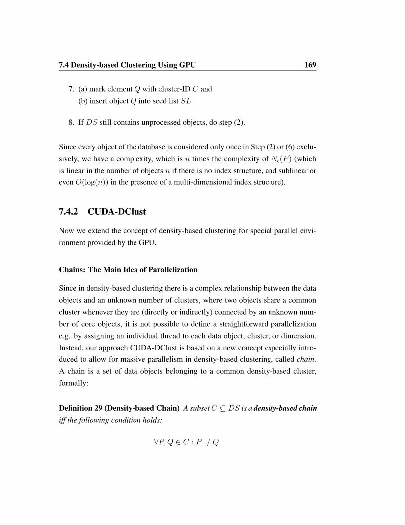
7.4 Density-based Clustering Using GPU 169
7. (a) mark element Q with cluster-ID C and(b) insert object Q into seed list SL.
8. If DS still contains unprocessed objects, do step (2).
Since every object of the database is considered only once in Step (2) or (6) exclu-sively, we have a complexity, which is n times the complexity of Nε(P ) (whichis linear in the number of objects n if there is no index structure, and sublinear oreven O(log(n)) in the presence of a multi-dimensional index structure).
7.4.2 CUDA-DClust
Now we extend the concept of density-based clustering for special parallel envi-ronment provided by the GPU.
Chains: The Main Idea of Parallelization
Since in density-based clustering there is a complex relationship between the dataobjects and an unknown number of clusters, where two objects share a commoncluster whenever they are (directly or indirectly) connected by an unknown num-ber of core objects, it is not possible to define a straightforward parallelizatione.g. by assigning an individual thread to each data object, cluster, or dimension.Instead, our approach CUDA-DClust is based on a new concept especially intro-duced to allow for massive parallelism in density-based clustering, called chain.A chain is a set of data objects belonging to a common density-based cluster,formally:
Definition 29 (Density-based Chain) A subsetC ⊆ DS is a density-based chainiff the following condition holds:
∀P,Q ∈ C : P ./ Q.

170 7. Data Mining Using Graphics Processors
Note that a cluster may be composed of several chains but each chain belongs toone single cluster only. In contrast to Definition 28, we do not require maximality.Using the concept of chains, we basically perform the task of cluster expansion,i.e. the transitive closure computation of the relation of direct density reachability.Thus, a chain can be considered as a tentative cluster with a tentative cluster-ID(which we call chain-ID). The idea is, instead of sequentially performing one
single cluster expansion like, for instance, in DBSCAN, we start many differentcluster expansions at the same time via different chains from different startingpoints. Of course CUDA-DClust has to register every collision between two ormore chains carefully. A collision means that CUDA-DClust has to notice thattwo chains actually participate in the same cluster. A detailed description of ourcollision handling is presented in the following.
We now introduce a concept for book-keeping all information that is essen-tial for collision handling, called collision matrix. A collision matrix CM is anupper triangular boolean matrix of size (p × p), where p is the number of chainsthat are expanded simultaneously. If a collision of chains i and j is detected, weset CMi,j := true if i < j and CMj,i := true otherwise. Since CM is small,we later run a sequential algorithm to determine transitive collisions. Finally, avalid cluster-ID is assigned to each chain and is distributed to the points in a par-allel fashion on GPU. Figure 7.6(a) illustrates parallelism based on the concept ofchains. Here, three density-based chains are processed in different thread groupsand may, therefore, be computed in a parallel fashion on different MPs of theGPU. Each MP is responsible for the expansion of one chain. The seed pointto be expanded is loaded into the shared memory in order to have it efficientlyaccessible for every thread in this thread group.
Besides the approach of chains, we introduce a second, but equally importantidea of parallelization. Whenever a point S is considered for determining its coreobject property and for marking its neighbors as potential new seed points, allpoints in Nε(S) must be determined. Therefor, a number of threads is generatedin order to process many potential neighbors Pi of S simultaneously. Note that,
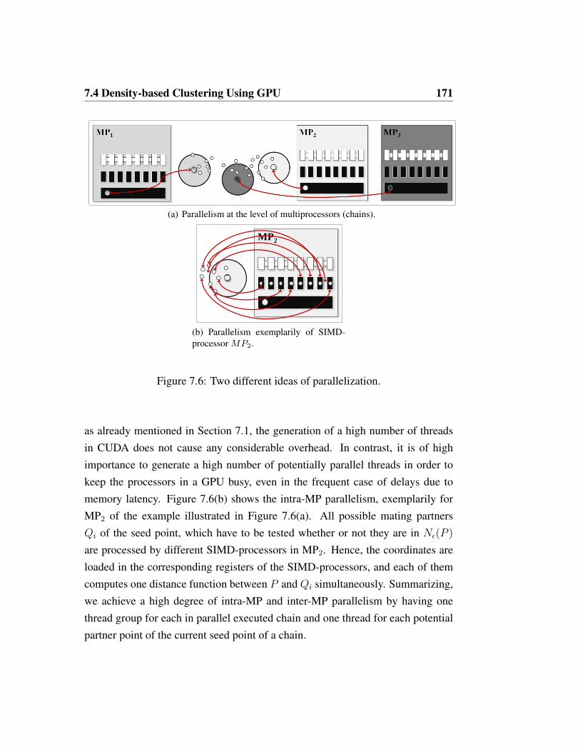
7.4 Density-based Clustering Using GPU 171
(a) Parallelism at the level of multiprocessors (chains).
MP2
(b) Parallelism exemplarily of SIMD-processor MP2.
Figure 7.6: Two different ideas of parallelization.
as already mentioned in Section 7.1, the generation of a high number of threadsin CUDA does not cause any considerable overhead. In contrast, it is of highimportance to generate a high number of potentially parallel threads in order tokeep the processors in a GPU busy, even in the frequent case of delays due tomemory latency. Figure 7.6(b) shows the intra-MP parallelism, exemplarily forMP2 of the example illustrated in Figure 7.6(a). All possible mating partnersQi of the seed point, which have to be tested whether or not they are in Nε(P )
are processed by different SIMD-processors in MP2. Hence, the coordinates areloaded in the corresponding registers of the SIMD-processors, and each of themcomputes one distance function between P and Qi simultaneously. Summarizing,we achieve a high degree of intra-MP and inter-MP parallelism by having onethread group for each in parallel executed chain and one thread for each potentialpartner point of the current seed point of a chain.
172 7. Data Mining Using Graphics Processors
In CUDA, multiples of 32 threads must be grouped into thread groups. As indi-cated in Section 7.1, threads of the same group are potentially executed in a fullysynchronous way in the same MP, may exchange information through the sharedmemory, and all threads of the same thread group can be synchronized when allthreads wait until all other threads of the same thread group have reached thesame point of execution. Therefore, it is obviously beneficial to collect all threadsbelonging to the same chain into one thread group.
The Cluster Expansion Kernel
The cluster expansion kernel is the main kernel method of CUDA-DClust. Itperforms the actual work, i.e. the determination of the core point property andthe transitive expansion of the clusters. We generate a high number of threads, allexecuting the cluster expansion kernel. Some other kernel methods for supportiveand cleaning tasks will be described in short later.
Consider the pseudocode presented in Algorithm 5a. Each thread group, gen-erated by the cluster expansion kernel starts with the ID of the seed point P thatis going to be processed. Its main tasks are, determine the neighbor-points, assertthe core object property of P , mark the neighbors as chain members, and recordpotential collisions in CM . A thread group starts by reading the coordinates ofP into the shared memory, and determining the minimum bounding rectangleMBRε(P ) of Nε(P ) allowing d-fold parallelism, where d is the dimension of thedata space. Then the threads are synchronized and a loop encounters all pointsQ ∈ PointSet from DS and considers them as potential neighbors in Nε(P ). Thisis done by all threads in the thread group allowing a maximum degree of intra-group parallelism. Therefore, this loop starts with the point with index thread-ID,and in each iteration, exactly the number of threads per thread group is added tothe index of the considered point Q. The further processing of Q by the proce-dure processObject depends on the core object property of P as clusters areexpanded from core objects only. However, at an early stage it may be unclear ifP is a core object. In any case, the distance δ between P and Q is determined. If
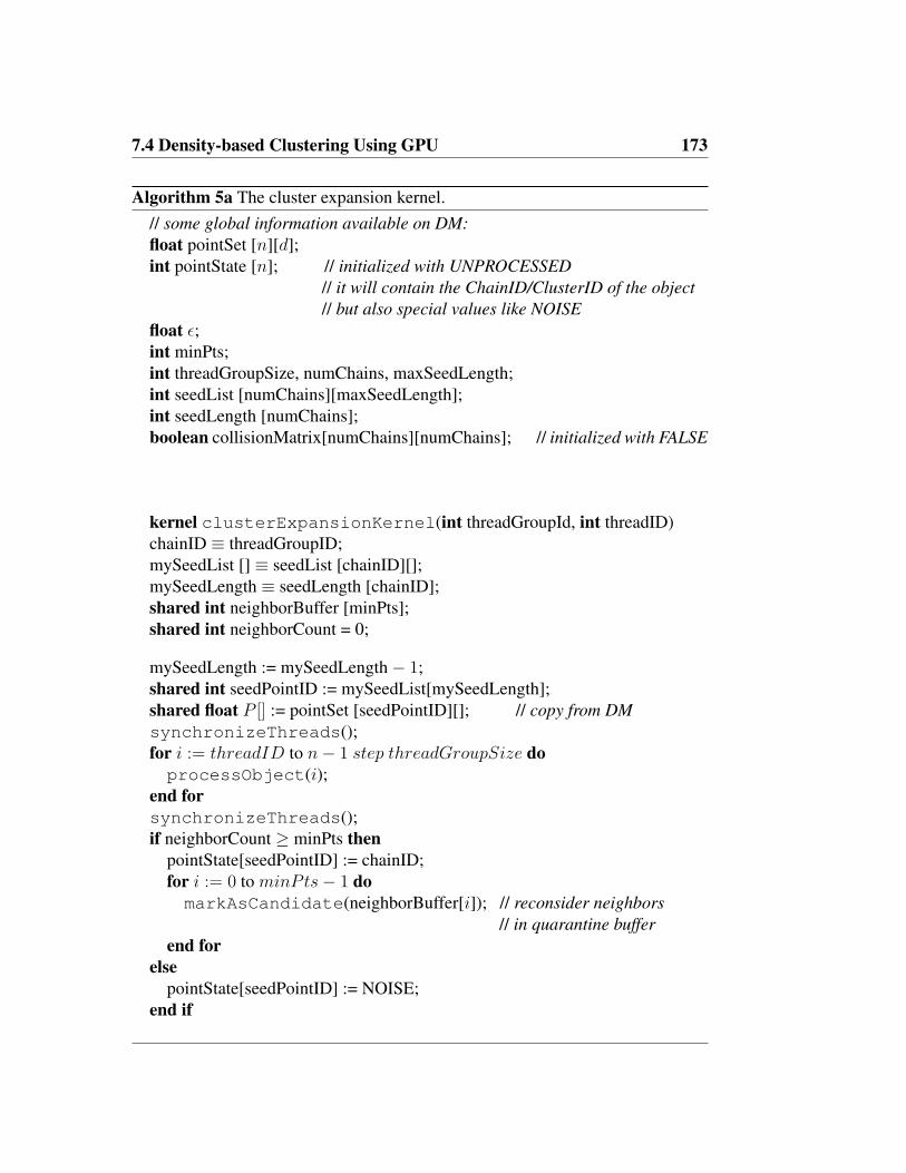
7.4 Density-based Clustering Using GPU 173
Algorithm 5a The cluster expansion kernel.// some global information available on DM:float pointSet [n][d];int pointState [n]; // initialized with UNPROCESSED
// it will contain the ChainID/ClusterID of the object// but also special values like NOISE
float ε;int minPts;int threadGroupSize, numChains, maxSeedLength;int seedList [numChains][maxSeedLength];int seedLength [numChains];boolean collisionMatrix[numChains][numChains]; // initialized with FALSE
kernel clusterExpansionKernel(int threadGroupId, int threadID)chainID ≡ threadGroupID;mySeedList [] ≡ seedList [chainID][];mySeedLength ≡ seedLength [chainID];shared int neighborBuffer [minPts];shared int neighborCount = 0;
mySeedLength := mySeedLength− 1;shared int seedPointID := mySeedList[mySeedLength];shared float P [] := pointSet [seedPointID][]; // copy from DMsynchronizeThreads();for i := threadID to n− 1 step threadGroupSize doprocessObject(i);
end forsynchronizeThreads();if neighborCount ≥ minPts then
pointState[seedPointID] := chainID;for i := 0 to minPts− 1 domarkAsCandidate(neighborBuffer[i]); // reconsider neighbors
// in quarantine bufferend for
elsepointState[seedPointID] := NOISE;
end if

174 7. Data Mining Using Graphics Processors
Algorithm 5b Procedure used by the cluster expansion kernel.procedure processObject(int i)register float Q [] := pointSet[i][];register float δ :=Distance(P,Q);if δ ≤ ε then
register int h = atomicInc(neighborCount);if h ≥ minPts thenmarkAsCandidate(i);
elseneighborBuffer[h] := i; // P not yet confirmed as core object,
// put Q in quarantine bufferend if
end if
Algorithm 5c Procedure used by the cluster expansion kernel.procedure markAsCandidate(int i)register int oldState = atomicCAS(pointState[i],UNPROCESSED,chainID);if oldState = UNPROCESSED then
register int h := atomicInc(mySeedLength, maxSeedLength);if h < maxSeedLength then
seedlist[h] := i;end if
elseif oldState 6= NOISE ∧ oldState 6= chainID then
if oldState < i thencollisionMatrix[oldState][i] := true; // collision!
elsecollisionMatrix[i][oldState] := true;
end ifend if
end if
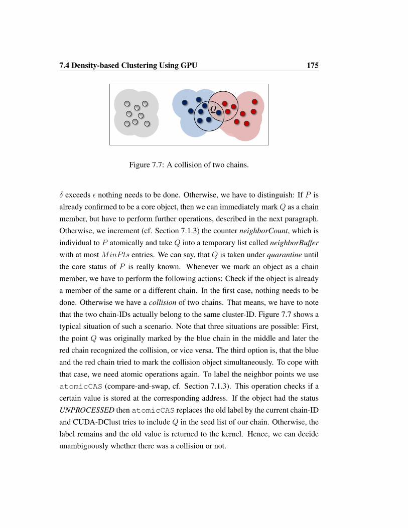
7.4 Density-based Clustering Using GPU 175
Figure 7.7: A collision of two chains.
δ exceeds ε nothing needs to be done. Otherwise, we have to distinguish: If P isalready confirmed to be a core object, then we can immediately mark Q as a chainmember, but have to perform further operations, described in the next paragraph.Otherwise, we increment (cf. Section 7.1.3) the counter neighborCount, which isindividual to P atomically and take Q into a temporary list called neighborBuffer
with at most MinPts entries. We can say, that Q is taken under quarantine untilthe core status of P is really known. Whenever we mark an object as a chainmember, we have to perform the following actions: Check if the object is alreadya member of the same or a different chain. In the first case, nothing needs to bedone. Otherwise we have a collision of two chains. That means, we have to notethat the two chain-IDs actually belong to the same cluster-ID. Figure 7.7 shows atypical situation of such a scenario. Note that three situations are possible: First,the point Q was originally marked by the blue chain in the middle and later thered chain recognized the collision, or vice versa. The third option is, that the blueand the red chain tried to mark the collision object simultaneously. To cope withthat case, we need atomic operations again. To label the neighbor points we useatomicCAS (compare-and-swap, cf. Section 7.1.3). This operation checks if acertain value is stored at the corresponding address. If the object had the statusUNPROCESSED then atomicCAS replaces the old label by the current chain-IDand CUDA-DClust tries to include Q in the seed list of our chain. Otherwise, thelabel remains and the old value is returned to the kernel. Hence, we can decideunambiguously whether there was a collision or not.

176 7. Data Mining Using Graphics Processors
Management of the Seed List
The seed list SL is the central data structure of density-based clustering. Its pur-pose is to provide a waiting queue for those objects, which are directly densityreachable from any object that has already been confirmed to be a core object ofthe current cluster, also named candidates. The core object property of the can-didates in the queue will be checked later, and a confirmed core object P will bereplaced by those objects, which are directly density reachable from P . SL is avery simple data structure: An unpriorized queue for a set of objects with the onlyoperations of storing and fetching an arbitrary object. In sequential density-basedclustering algorithms such as DBSCAN or OPTICS, only one seed list must bemaintained. In contrast, CUDA-DClust simultaneously performs cluster expan-sions of a moderately high number of chains, and, therefore, multiple seed listsmust be managed, which potentially causes space problems. The index numberof the actual seed list that is used by a thread group can be determined from itsTG-ID (which simultaneously serves as Chain-ID). To facilitate the readability ofthe code, at the beginning of the kernel ClusterExpansion, these simplificationsare introduced by equivalence associations using the symbol ≡. These are onlymeant as shortcuts, and no copying of data is needed.
For the insertion of objects into SL the operation atomicInc (for incre-ment) has to be used because some candidates may be simultaneously insertedby different threads of the same thread group. The space in each seed list in thedevice memory is limited by a parameter (maxSeedLength). In our experiments,we used 1,024 points per seed list. In case of a list overflow, new points are onlymarked by the current chain-ID but not inserted into the seed list. We use twodifferent counters to keep track of the number of discarded candidates. Using aspecial kernel method, called SeedRefill Kernel we can search for candidates thathave been discarded.

7.4 Density-based Clustering Using GPU 177
Load Balancing
Since a number of seeds is expanded simultaneously and a number of chains isprocessed in parallel, it naturally happens that one of the chains is completed be-fore the others. In this case, we start a new chain from an unprocessed object.If no such object is available, we split a chain, i.e. one of the objects from SL
of a randomly selected chain is removed and we start a new chain with that can-didate. Thereby, an almost constant number of threads working in the system isguaranteed, all with approximately the same workload.
The Main Program for CPU
Apart from initialization, the main program consist merely of a loop starting threedifferent kernel methods on the GPU, until no more unprocessed data objects existany more:
1. Transfer the dataset from main memory to device memory;
2. Create NumChains new chains from randomly selected points of DS;
3. StartKernel (ClusterExpansion);
4. Transfer the states of the chains from device memory to main memory;
5. If necessary, StartKernel (NewSeeds);
6. If necessary, StartKernel (SeedRefill);
7. If unprocessed objects exist, continue with step (3);
8. Transfer the result (cluster-IDs) from device memory to main memory.

178 7. Data Mining Using Graphics Processors
CUDA-DClust* - The Indexed Version of CUDA-DClust
The performance of CUDA-DClust can be significantly improved by the multi-dimensional index structure presented in Section 7.2, supporting the search ofpoints in the ε-neighborhood of some object P ∈ Nε(P ). To receive the indexedversion of CUDA-DClust named CUDA-DClust*, our index structure must beconstructed in a bottom-up way by fractionated sorting of the data DS beforestarting the actual clustering method. When transferring DS from the main mem-ory into the device memory in the initialization step of CUDA-DClust, CUDA-DClust* has to transfer the directory additionally. Compared to the size of DS,the directory is always small. The most important change in our cluster expansionkernel regards the determination of Nε(P ) of some given seed object P , whichis done by exploiting SIMD-parallelism inside a MP. In CUDA-DClust, this wasdone by a set of threads inside a thread group, each of which iterated over a dif-ferent part of DS. In CUDA-DClust*, one of the threads iterates in a set of nestedloops over those nodes of the index structure, which represent regions of DS thatintersect Nε(P ). In the innermost loop, we have one set of points correspond-ing to a data page of the index structure, which is processed by exploiting theSIMD-parallelism, like in CUDA-DClust.
7.4.3 Experimental Evaluation
To evaluate the performance of density-based clustering on GPU, we execute dif-ferent experiments. First, we evaluate CUDA-DClust vs. DBSCAN without indexsupport and CUDA-DClust* vs. DBSCAN with index support w.r.t. the size ofthe datasets. Second, we analyze the impact of the parameters MinPts and ε.Finally, we perform an evaluation w.r.t. the data dimensionality. All test dataare synthetic feature vectors containing 20 randomly generated Gaussian clusters.Unless otherwise mentioned, the algorithms are parameterized with ε = 0.05 andMinPts = 4. These parameters are used in an analogous way like the correspon-dent parameters of the sequential DBSCAN algorithm. The time needed for index
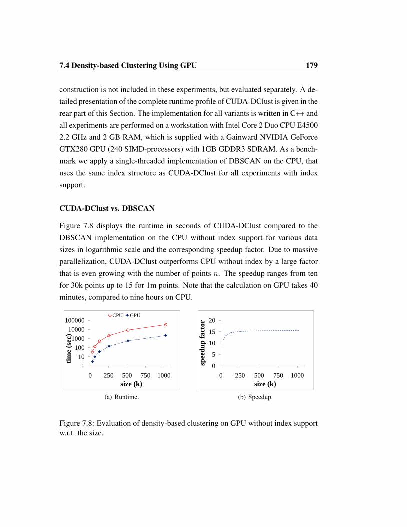
7.4 Density-based Clustering Using GPU 179
construction is not included in these experiments, but evaluated separately. A de-tailed presentation of the complete runtime profile of CUDA-DClust is given in therear part of this Section. The implementation for all variants is written in C++ andall experiments are performed on a workstation with Intel Core 2 Duo CPU E45002.2 GHz and 2 GB RAM, which is supplied with a Gainward NVIDIA GeForceGTX280 GPU (240 SIMD-processors) with 1GB GDDR3 SDRAM. As a bench-mark we apply a single-threaded implementation of DBSCAN on the CPU, thatuses the same index structure as CUDA-DClust for all experiments with indexsupport.
CUDA-DClust vs. DBSCAN
Figure 7.8 displays the runtime in seconds of CUDA-DClust compared to theDBSCAN implementation on the CPU without index support for various datasizes in logarithmic scale and the corresponding speedup factor. Due to massiveparallelization, CUDA-DClust outperforms CPU without index by a large factorthat is even growing with the number of points n. The speedup ranges from tenfor 30k points up to 15 for 1m points. Note that the calculation on GPU takes 40minutes, compared to nine hours on CPU.
100010000
100000
sec)
CPU GPU
110
100
0 250 500 750 1000
time
(s
size (k)
(a) Runtime.
10
15
20
up fa
ctor
0
5
10
0 250 500 750 1000
spee
du
size (k)
(b) Speedup.
Figure 7.8: Evaluation of density-based clustering on GPU without index supportw.r.t. the size.

180 7. Data Mining Using Graphics Processors
CUDA-DClust* vs. Indexed DBSCAN
The following experiments are performed with index support as introduced inSection 7.2. The runtime of CUDA-DClust* and the indexed version of DBSCANon CPU and speedup are presented in Figure 7.9. CUDA-DClust* outperforms thebenchmark again by a large factor, that is proportional to the size of the dataset.In this evaluations the speedup ranges from 3.5 for 30k points to almost 15 for2m points. A guaranteed speedup factor of at least ten is obtained by datasetsconsisting of more than 250k points.
100010000
100000
sec)
CPU GPU
110
100
0 500 1000 1500 2000
time
(s
size (k)
(a) Runtime.
10
15
20
up fa
ctor
0
5
10
0 500 1000 1500 2000
spee
du
size (k)
(b) Speedup.
Figure 7.9: Evaluation of density-based clustering on GPU with index supportw.r.t. the size.
Impact of the Parameter MinPts
In these experiments we test the impact of the parameter MinPts on the perfor-mance of CUDA-DClust* against the indexed version of DBSCAN on CPU. Weuse a synthetic dataset with a fixed number of about 260k 8-dimensional pointsand choose ε = 0.05. The parameter MinPts is evaluated in a range from 4 to2,048. Figure 7.10 shows that the runtime of CUDA-DClust* increases for largerMinPts values. For 4 ≤ MinPts ≤ 512 the speedup factor remains relativelystable between ten and five. Then the speedup decreases significantly. However

7.4 Density-based Clustering Using GPU 181
CUDA-DClust* outperforms the implementation on CPU even for largeMinPts-values by a factor of two. The speedup decline can be explained by a closer lookat the implementation details of CUDA-DClust* (cf. Section 7.4.2). It can be seenthat the first MinPts − 1 found neighbors have to be buffered, because they cannot be marked before it is guaranteed that the seed point is also a core point. As allthreads that are executed in parallel have to share the limited shared memory, lessthreads can be executed in parallel if a high number of points have to be bufferedin addition.
1
10
100
1000
10000
100000
0 500 1000 1500 2000 2500
tim
e (s
ec)
MinPts
CPU GPU
(a) Runtime.
0
5
10
15
20
0 500 1000 1500 2000 2500
spee
du
p f
act
or
MinPts
(b) Speedup.
Figure 7.10: Evaluation of CUDA-DClust* w.r.t. MinPts.
Impact of the Parameter ε
We also evaluated the impact of the second DBSCAN parameter ε on CUDA-DClust* using a synthetic dataset consisting of 260k 8-dimensional points andfixedMinPts = 4. We test the impact of ε for values that range from 0.02 to 0.10and present the results in Figure 7.11. Evidently, the impact of ε is negligible, asthe range of the corresponding speedup factor is almost stable between nine andten.

182 7. Data Mining Using Graphics Processors
1001000
10000100000
sec)
CPU GPU
110
100
0,00
time
(
ε0.00 0.02 0.04 0.06 0.08 0.10
(a) Runtime.
10
15
20
p fa
ctor
0
5
10
0,00
spee
dup
ε0.00 0.02 0.04 0.06 0.08 0.10
(b) Speedup.
Figure 7.11: Evaluation of CUDA-DClust* w.r.t. ε.
Evaluation of the Dimensionality
Here, we provide an evaluation w.r.t. the dimensionality of the data, ranging from4 to 64. Again, we use our algorithm CUDA-DClust* and perform all tests on thesynthetic dataset consisting of 260k 8-dimensional points clustered with defaultparameter-settings for ε and MinPts. Figure 7.12 illustrates that CUDA-DClust*outperforms the benchmark by factors of about seven to twelve depending on thedimensionality of the data. In our DBSCAN implementation the dimensionality isalready known at compile time. Hence, optimization techniques of the compilerhave an impact on the performance of the CPU version. Obviously, also the sizeof the data structures for the seed points in the GPU implementation is affectedby the dimensionality and hence influences the performance of CUDA-DClust*,as the data structures are stored in the shared memory. This overhead affects thenumber of threads that can be executed in parallel on the GPU.
Evaluation of the Index Construction
All experiments do not include the time that is needed for constructing the indexstructure (described in Section 7.2) so far. Table 7.2 displays the time needed toconstruct the index, the runtime of CUDA-DClust and relates these two terms to

7.4 Density-based Clustering Using GPU 183
100010000
100000
sec)
CPU GPU
110
100
0 10 20 30 40 50 60
time
(s
dimensionality
(a) Runtime.
10
15
20
up fa
ctor
0
5
10
0 10 20 30 40 50 60
spee
du
dimensionality
(b) Speedup.
Figure 7.12: Evaluation of CUDA-DClust* w.r.t. the dimensionality.
each other for various sizes and dimensions of synthetic datasets. All experimentsindicate that the time for building the index structure is negligible and indepen-dent of the parameter-setting by a fraction of lower than 5%. Further analysisdemonstrate that larger datasets show an even smaller value of lower than 2%.
Table 7.2: Evaluation of the Index Construction for CUDA-DClust*.
n DIM INDEX GPU INDEX / GPU65k 8 0.1 s 2.2 s 4.5 %
130k 8 0.2 s 5.8 s 3.4 %260k 8 0.4 s 16.5 s 2.4 %260k 16 0.6 s 38.6 s 1.6 %260k 32 1.0 s 45.9 s 2.2 %260k 64 1.8 s 111.6 s 1.6 %520k 8 0.8 s 52.1 s 1.5 %1m 8 1.7 s 182.4 s 0.9 %2m 8 3.6 s 681.8 s 0.5 %

184 7. Data Mining Using Graphics Processors
Runtime Profiling
In this section, we present a detailed runtime profile of CUDA-DClust* concern-ing different parts of the algorithm that is evaluated on two different syntheticdatasets. The corresponding charts are depicted in Figure 7.13. The left diagramillustrates the distribution of the execution time of the program parts cluster expan-sion kernel, new seeds kernel, collision matrix and seed refill kernel on a datasetconsisting of 520k 8-dimensional points and the right diagram for 4m points, re-spectively. Thus the bulk of performance is executed by the cluster expansionkernel. The auxiliary program parts and computations on CPU only consume asmall fraction of the complete runtime as desired. Remark that the CPU is not re-served during the execution of the cluster expansion kernel, that requires the mainpart of the computation. Hence, the CPU can process multiple other jobs whilethe algorithm is executed by the cluster expansion kernel. In all experiments thetime needed to divide the clustering process and the time to integrate the result forboth algorithms CUDA-DClust and CUDA-DClust* is negligible.
cluster expansion kernel
new seeds kernel
cluster expansion kernel
new seeds kernel
collision matrix
seed refill kernel
cluster expansion kernel
new seeds kernel
collision matrix
seed refill kernel
Figure 7.13: Runtime profile of CUDA-DClust* for two different datasets.
7.4.4 Conclusions
We proposed CUDA-DClust, a novel algorithm for very efficient density-basedclustering supported by the computing power of the GPU. This architecture al-lows for extreme parallelization at very low cost. CUDA-DClust combines sev-eral concepts to exploit the special characteristics of the GPU for clustering, as
7.5 Partitioning Clustering on GPU 185
parallel cluster expansion supported by the concept of chains, parallel nearestneighbor search that can even be accelerated by the use of a hierarchical indexstructure, and effective load balancing among the microprocessors. Our experi-ments demonstrate that CUDA-DClust outperforms the algorithm DBSCAN onCPU by an order of magnitude and yields an equally accurate clustering. The im-pressive results can even be increased by the use of an appropriate index structure,which yields to our second proposed algorithm CUDA-DClust*.
7.5 Partitioning Clustering on GPU
Finally, we describe the idea of performing a second paradigm of clustering,namely partitioning k-means clustering, on GPU.
7.5.1 The Sequential Procedure of k-means Clustering
A well-established partitioning clustering method is the k-means clustering al-gorithm [72]. k-means requires a metric distance function in vector space. Inaddition, the user has to specify the number of desired clusters k as an input pa-rameter. Usually k-means starts with an arbitrary partitioning of the objects into kclusters. After this initialization, the algorithm iteratively performs the followingtwo steps until convergence: (1) Update centers: For each cluster, compute themean vector of its assigned objects. (2). Re-assign objects: Assign each object toits closest center. The algorithm converges as soon as no object changes its clusterassignment during two subsequent iterations.
Figure 7.14 illustrates an example run of k-means for k = 3 clusters. Fig-ure 7.14(a) shows the situation after random initialization. In the next step, everydata point is associated with the closest cluster center (cf. Figure 7.14(b)). Theresulting partitions represent the Voronoi cells generated by the centers. In thefollowing step of the algorithm, the center of each of the k clusters is updated, asshown in Figure 7.14(d). Finally, assignment and update steps are repeated untilconvergence.

186 7. Data Mining Using Graphics Processors
In most cases, fast convergence can be observed. The optimization function ofk-means is well defined. The algorithm minimizes the sum of squared distancesof the objects to their cluster centers. However, k-means is only guaranteed toconverge towards a local minimum of the objective function. The quality of theresult strongly depends on the initialization. Finding that clustering with k clus-ters minimizing the objective function actually is a NP-hard problem, for detailssee e.g. [75]. In practice, it is therefore recommended to run the algorithm sev-eral times with different random initializations and keep the best result. For largedatasets, however, often only a very limited number of trials is feasible. Paralleliz-ing k-means in GPU allows for a more comprehensive exploration of the searchspace of all potential clusterings and thus provides the potential to obtain a goodand reliable clustering even for very large datasets.
(a) Initialization. (b) Assignment. (c) Recalculation. (d) Termination.
Figure 7.14: Sequential partitioning clustering by the k-means algorithm.
7.5.2 CUDA-k-Means
In k-means, most computing power is spent in step (2) of the algorithm, i.e. re-assignment which involves distance computation and comparison. The number ofdistance computations and comparisons in k-means is O(k · i ·n), where i denotesthe number of iterations and n is the number of data points.

7.5 Partitioning Clustering on GPU 187
The CUDA-k-MeansKernel
In k-means, the cluster assignment of each data point is determined by comparingthe distances between the point and each cluster center. This work is performedin parallel by the CUDA-k-meansKernel. The idea is, instead of (sequentially)performing cluster assignment of one single data point, many different cluster as-signments are started simultaneously. In detail, one single thread per data point isgenerated, all executing the CUDA-k-meansKernel. Every thread which is gen-erated from the CUDA-k-meansKernel (cf. in Algorithm 6) starts with the ID ofa data point x that is going to be processed. Its main tasks are, to determine thedistance to the next center and the ID of the corresponding cluster.
A thread starts by reading the coordinates of the data point x into the register.The distance of x to its closest center is initialized by∞ and the assigned clusteris therefore set to null. Then a loop encounters all c1, c2, . . . , ck centers andconsiders them as potential clusters for x. This is done by all threads in the samethread group allowing a maximum degree of intra-group parallelism. Finally, thecluster whose center has the minimum distance to the data point x is reportedtogether with the corresponding distance value using synchronized writing.
The Main Program for CPU
Apart from initialization and data transfer from main memory to device memory,the main program consists of a loop starting the CUDA-k-meansKernel on GPUuntil the clustering converges. After the parallel operations are completed by allthreads of the group, the following steps are executed in each cycle of the loop:
1. Copy distance of processed point x to the nearest center from device intomain memory.
2. Copy cluster, x is assigned to, from device memory into main memory.
3. Update centers.
4. Copy updated centers to device memory.

188 7. Data Mining Using Graphics Processors
Algorithm 6 Parallel algorithm for k-means on GPU.algorithm CudaKMeans(datasetDS, int k) // host program executed on CPUdeviceMem float DS ′[][] := DS[][]; // allocate memory in DM for DSthreads := n; // number of points in DStpg := 64; // threads per groupdeviceMem float Centroids[][] := initCentroids(); // allocate memory in DM
// for the initial centroidsdouble actCosts :=∞; // initial costs of clustering
repeatprevCost := actCost;startThreads(CudaKMeansKernel, threads, tpg); // one thread per pointwaitForThreadsToFinish();float minDist := minDistances[threadID]; // copy distance to nearest
// centroid from DM into MMfloat cluster := clusters[threadID]; // copy assigned cluster
// from DM into MMdouble actCosts := calculateCosts(); // update costs of clusteringdeviceMem float Centroids[][] := calculateCentroids();
// copy updated centroids to DMuntil |actCost− prevCost| < threshold
kernel CudaKMeansKernel(int threadID)register float x[] := DS ′[threadID][]; // copy x from DM into registerfloat minDist :=∞; // distance of x to the next centroidint cluster := null; // ID of the next centroid (cluster)for i := 1 to k do
register float c[] := Centroids[i][] // copy actual centroid// from DM into register
double dist := distance(x,c);if dist < minDist thenminDist := dist;cluster := i;
end ifend forreport(minDist, cluster); // report assigned cluster and distance
// using synchronized writing
7.5 Partitioning Clustering on GPU 189
7.5.3 Experimental Evaluation
To analyze the efficiency of k-means clustering on GPU, we present experimentsw.r.t. different dataset sizes, number of clusters and dimensionality of the data.As benchmark we apply a single-threaded implementation of k-means on CPU todetermine the speedup of the implementation of k-means on GPU. As the numberof iterations may vary in each run of the experiments, all results are normalizedby a number of 50 iterations both on GPU and CPU implementation of k-means.All experiments are performed on synthetic datasets as described in detail in eachof the following settings.
Evaluation of the Dataset Sizes
For these experiments we created 8-dimensional synthetic datasets of differentsizes, ranging from 32k to 2m data points. The datasets consist of differentnumbers of random clusters, generated like DS1, specified in Table 7.1. Fig-ure 7.15(a) displays the runtime in seconds in logarithmic scale and the corre-sponding speedup factors of CUDA-k-means and the benchmark method on CPUfor different number of data points. The time needed for data transfer from CPUto GPU and back has been included. The corresponding speedup factors are givenin Figure 7.15(b). Once again, these experiments support the evidence that theperformance of data mining approaches on GPU outperform classic CPU ver-sions by significant factors. Whereas a speedup of approximately 10 to 100 canbe achieved for relatively small number of clusters (data objects), we obtain aspeedup of about 1000 for 256 clusters, that is even increasing with the number ofdata objects.
Evaluation of the Number of Clusters
We performed several experiments to validate CUDA-k-means w.r.t. the numberof clusters k. Figure 7.15(c) shows the runtime in seconds of CUDA-k-meanscompared with the implementation of k-means on CPU on 8-dimensional syn-

190 7. Data Mining Using Graphics Processors
100010000
c)
CPU (32 clusters) CPU (64 clusters) CPU (256 clusters)
GPU (32 clusters) GPU (64 clusters) GPU (256 clusters)
110
100
0 500 1000 1500 2000
time
(sec
size (k)
(a) Runtime for different dataset sizes.
7501000
fact
or
32 clusters 64 clusters 256 clusters
0250500
0 500 1000 1500 2000
spee
dup
size (k)
(b) Speedup for different dataset sizes.
1001000
10000
c)
CPU (32k points) CPU (500k points) CPU (2m points)
GPU (32k points) GPU (500k points) GPU (2m points)
01
10100
0 50 100 150 200 250time
(sec
k
(c) Runtime for different number of clusters.
7501000
fact
or
32 points 500k points 2m points
0250500
0 50 100 150 200 250
spee
dup
k
(d) Speedup for different number of clusters.
1001000
10000
ec)
CPU GPU
01
10
0 50 100 150 200 250time
(se
dimensionality
(e) Runtime for different dimensionalities.
500750
1000
p fa
ctor
0250500
0 50 100 150 200 250
spee
dup
dimensionality
(f) Speedup for different dimensionalities.
Figure 7.15: Evaluation of k-means clustering on CPU and GPU w.r.t. the size ofdifferent datasets, the number of clusters, and different dimensionalities.

7.5 Partitioning Clustering on GPU 191
thetic datasets that contain different number of clusters, ranging from 32 to 256,again together with the corresponding speedup factors in Figure 7.15(d).
The experimental evaluation of k on a dataset that consists of 32k points re-sults in a maximum performance benefit of more than 800 compared to the bench-mark implementation. For 2m points the speedup ranges from nearly 100 up toeven more than 1,000 for a dataset that comprises 256 clusters. In this case thecalculation on the GPU takes approximately five seconds, compared to almostthree hours on CPU. Therefore, we determine that due to massive parallelization,CUDA-k-means outperforms the CPU implementation by large factors, that areeven growing with k and the number of data objects n.
Evaluation of the Dimensionality
These experiments provide an evaluation w.r.t. the dimensionality of the data. Weperform all tests on synthetic data consisting of 16k data objects. The dimension-ality of the test datasets vary in a range from 4 to 256. Figure 7.15(f) illustrates thatCUDA-k-means outperforms the benchmark method k-means on CPU by factorsof 230 for 128-dimensional data to almost 500 for 8-dimensional data. On GPUand CPU, the dimensionality affects possible compiler optimization techniques,like loop unrolling as already shown in the experiments for the evaluation of thesimilarity join on the GPU (cf. Section 7.3.3).
7.5.4 Conclusions
We demonstrated how Graphics processing Units (GPU) can effectively supporthighly complex data mining tasks. In particular, we focused on the iterative al-gorithm k-means and proposed algorithms illustrating how to effectively supportclustering on GPU. Our proposed algorithm is accustomed to the special environ-ment of the GPU which is most importantly characterized by extreme parallelismat low cost. Our experimental evaluation emphasizes the potential of the GPU forhigh-performance data mining.

192 7. Data Mining Using Graphics Processors

Chapter 8
Conclusions
The rapidly increasing amount of data stored in databases requires effective andefficient data mining methods to gain new information contained in the collecteddata. Clustering is one of the primary data mining tasks and aims at detectingsubgroups of similar data objects. This thesis contributes to the fields of min-ing structured datatypes and proposes opportunities for boosting the data miningprocess by the intelligent adoption of Graphics Processing Units (GPUs). In Sec-tion 8.1, a detailed summary of our contributions is given. This thesis is concludedby some potential ideas for future work in Section 8.2.
8.1 Summary
Many data contain some kind of hierarchical relationship. That means that datamining approaches can reveal the information present in this data w.r.t. differentlevels. Hierarchical clustering has therefore become very popular in various sci-entific domains, such as molecular biology, medicine or economy. In this thesis,we contributed two novel hierarchical clustering algorithms – ITCH (Information-theoretic Cluster Hierarchies) and GACH (Genetic Algorithm for Finding Clus-ter Hierarchies). ITCH is a hierarchical information-theoretic clustering methodthat has the following advantages: It uses a Gaussian probability density function
194 8. Conclusions
(PDF) as representative for each cluster. This is returned as the result of the clus-tering method but also consequently used as an optimization criterion during thealgorithm. Furthermore, each node in the hierarchy represents a meaningful clus-ter. This is achieved by an adaptation of the Minimum Description Length (MDL)principle for the hierarchical case. Outliers are flexibly handled by assigning themto higher levels of the cluster hierarchy. Outliers which are completely dissimilarto all objects in the database may be assigned to the root of the hierarchy; otherpoints which are outliers to a lesser degree and just do not fit to any very spe-cific cluster at a very detailed view may be assigned to intermediate layers of thehierarchy. Finally, ITCH is effective, efficient and fully automatic, i.e. difficultand critical parameter settings are avoided. The second hierarchical clusteringalgorithm, presented in this thesis, is called GACH. GACH is a genetic-based al-gorithm which combines the benefits of genetic algorithms, information theoryand model-based clustering being an efficient and accurate hierarchical clusteringtechnique. It uses a MDL-based fitness function. Hence, it can be easily appliedto real world applications without requiring any background knowledge by theuser about the data, like e.g. the real number of clusters. Due to the fact thatGACH integrates an EM-like strategy, the content of all clusters is described byan intuitive description in form of a PDF. As ITCH, GACH assigns outliers toappropriate inner nodes of the hierarchy, depending on their degree of outlierness.Our experimental evaluation demonstrate that GACH outperforms a multitude ofother clustering approaches in terms of accuracy. In fact, we have obtained betterresults concerning different quality measures.
Besides hierarchical data mining, the analysis of data that are composed ofattributes concerning different domains has turned out to be among the top 10challenging problems in data mining. This thesis contributes a novel integrativeclustering algorithm that addresses the question how to find a good partitioning ofdata that have both numerical and categorical attributes. Most of the existing clus-tering approaches require prior knowledge on the data that specifies the numberof clusters or defines the weighting of the numerical and categorical information.

8.1 Summary 195
Here, we gave a solution to avoid difficult parameter settings in integrative clus-tering which was guided by the information-theoretic idea of data compression.For this purpose, we defined iMDL, an alternative for the classic MDL princi-ple. The data partitioning can be used for efficient coding, and the achievablecompression rate thus defines an objective function for the integrative clusteringproblem. On top of the idea of data compression we have proposed INTEGRATE,an information-theoretic integrative clustering method which is a k-means basedapproach for mixed type data that fulfills the following requirements. First, basedon the MDL principle, INTEGRATE allows for a natural weighting of numeri-cal and categorical information. Second, there is no need for difficult parametersettings which makes INTEGRATE fully automatic. Third, being the result of anoptimization process maximizing the achievable data compression, INTEGRATEuses the numerical and categorical information most effectively. And finally, itshows high efficiency and is therefore scalable to large datasets.
Performing data mining on complex data that can not be easily described byfeature vectors was another challenging problem during this work. However, in-spired by the success of the skyline operator for multi-criteria decision making,we demonstrated that the skyline of a dataset is a very useful representation cap-turing the most interesting characteristics. And therefore, data mining on skylinesis very promising for knowledge discovery. With SkyDist, a similarity measurefor comparing different skylines, we proposed the first approach to data mining onskyline objects. We presented a baseline Monte-Carlo Sampling approach, calledMCSkyDist that approximates the distance and an exact sweep-line based compu-tation, named SLSkyDist. We showed, that SkyDist can easily be integrated intomany data mining techniques. Real world case studies on clustering skylines thatrepresent interesting offers of an automotive market or that describe the perfor-mance profile of basketball players, demonstrated that data mining on skylines,enabled by SkyDist, yields interesting novel knowledge.
Finally, we presented different contributions to the field of graph mining.Among the aforementioned data structures, graphs or networks are the most gen-

196 8. Conclusions
eral ones, as almost every relationship can be modeled by graphs. In particular,we worked on a large real case study on brain networks of patients with somato-form pain disorder. The brain network models were constructed out of fMRI scantime series (a special form of neuroimaging) of six somatoform patients and fourhealthy controls. Each edge inside the network represents a significant degree ofco-activation between different brain regions. On these network models, we haveapplied the heuristic frequent subgraph algorithm GREW and FANMOD, an ex-haustive sampling method for frequent subgraph discovery. The resulting patternsrepresent groups of brain compartments that covary in their activity during theprocess of pain stimulation. We evaluated the appearance of frequent subgraphsfor the group of patients and the healthy controls, respectively. Our results let ussuspect that somatoform pain disorder is caused by an additional pathogeneousactivity, not by a missing physiological activity. So far we have cared about thetopology of the network, but ignore the temporal order of these interactions. Totake this aspect into account, we defined an approach for dynamic graph miningand applied it on biological yeast networks. To achieve real dynamic networks,we co-integrated gene expression and protein interaction data from the organismS.cerevisiae. The information about the presence of an edge at a particular timestep is modeled by so-called existence strings. We have defined an efficient algo-rithm for frequent dynamic subgraph discovery in an on-top fashion, meaning thatwe search a set of frequent static subgraphs for dynamic patterns. To provide theenumeration of static patterns, existing subgraph mining algorithms can be eas-ily integrated into our framework. The dynamic patterns are efficiently computedusing the idea of suffix trees. The resulting patterns represent groups of proteinsthat occur frequently within a protein interaction network and in which pairs ofproteins are co-regulated in the same temporal order.
In the second part of this thesis, we contributed to the efficiency aspect of datamining algorithms. Many computations are extremely time consuming, especiallyin the presence of large databases. We presented solutions by the help of graphicsprocessors that can effectively support highly complex data mining tasks. In par-
8.2 Outlook 197
ticular, we demonstrated how to boost the clustering process and presented ideasfor accelerating the similarity search. We selected two well-known clusteringalgorithms, the density-based algorithm DBSCAN and the iterative partitioningalgorithm k-means and proposed approaches illustrating how to effectively sup-port clustering on GPU. Our proposed algorithms are accustomed to the specialenvironment of the GPU which is most importantly characterized by extreme par-allelism at low cost. In addition, we proposed a parallel version of the similarityjoin and an index structure for efficient similarity search. Going beyond the pri-mary scope of this idea, these building blocks are applicable to support a widerange of data mining tasks, including outlier detection, association rule miningand classification. Our extensive experimental evaluation emphasizes the poten-tial of the GPU for high-performance data mining.
8.2 Outlook
At the end of this thesis, the potentials of the proposed methods for future researchare emphasized.
• While much work has been done in identifying cluster structures that are de-scribed by Gaussian Mixture Models, the field of detecting structures thatform relationships of PDFs of arbitrary type is almost unexplored. Extend-ing the coding scheme for Gaussian PDFs to mixture models of the Expo-nential Power Distribution type would therefore be a next step.
• Our algorithms ITCH and GACH for information-theoretic mining of clus-ter hierarchies are based on a hierarchical extension of the MDL principle.For simplicity the coding scheme is restricted to the diagonal covariancematrix. In order to apply our algorithms on arbitrary oriented clusters, weplan to integrate the coding of the complete covariance matrix w.r.t. hierar-chical cluster relationships.

198 8. Conclusions
• For GACH, we used the heuristic approach of genetic algorithms. Anotherpromising probabilistic heuristic concept would be simulated annealing. Ineach step of the simulated annealing process, the current solution for thehierarchical clustering problem is replaced by a random solution. The newsolution may then be accepted with a probability that depends both on thedifference between the corresponding hMDL value and also on a globalparameter T (called the temperature), that is gradually decreased during theprocess.
• Another interesting idea would be to amplify the field of integrative datamining. While our proposed algorithm INTEGRATE is designed to handledata that consists of numerical and categorical attributes, one might alsobe interested in incorporating data types like e.g. graph-structures. Usinga variety of different information for the data mining process yields to amaximum of knowledge extraction. For example, a clustering method thatcombines categorical and graph-structured data can be used highly effectivefor mining social network data.
• For high efficient data mining, future research could be guided in the fol-lowing directions: Besides similarity search and clustering there is a highnumber of data mining processes that are often hard to apply on large real-world data. Therefore, it would be beneficial to develop further algorithmsto support more specialized data mining tasks on GPU, including for exam-ple subspace and correlation clustering and medical image processing.

List of Figures
1.1 The KDD process. . . . . . . . . . . . . . . . . . . . . . . . . . 21.2 Example for clustering. . . . . . . . . . . . . . . . . . . . . . . . 41.3 Example for feature transformation. . . . . . . . . . . . . . . . . 51.4 Growth trend of NVIDIA GPU vs. CPU. . . . . . . . . . . . . . . 9
2.1 A dendrogram for a given sample dataset. . . . . . . . . . . . . . 142.2 A reachability plot for a given sample dataset. . . . . . . . . . . . 182.3 Coding scheme for parameter-free clustering. . . . . . . . . . . . 262.4 Illustration of the rightmost extension used in gSpan. . . . . . . . 282.5 The NVIDIA GeForce 8800 GTX graphics processor. . . . . . . . 31
3.1 Contributions of the EM-based clustering method ITCH. . . . . . 373.2 Illustrative example of the hierarchical cut. . . . . . . . . . . . . . 413.3 Optimization of coding scheme for the location parameter. . . . . 443.4 Restructure operations of ITCH. . . . . . . . . . . . . . . . . . . 523.5 Synthetic datasets for the evaluation of ITCH. . . . . . . . . . . . 553.6 Competitive evaluation of ITCH on a synthetic hierarchical dataset. 563.7 Competitive evaluation of ITCH on a synthetic flat dataset. . . . . 583.8 Competitive evaluation of ITCH on the real-world Glass dataset. . 593.9 Competitive evaluation of ITCH on the real-world Cancer dataset. 613.10 Stability of ITCH. . . . . . . . . . . . . . . . . . . . . . . . . . . 623.11 Motivation behind GACH. . . . . . . . . . . . . . . . . . . . . . 643.12 Summarization of the mutation operators used for GACH. . . . . 68
200 LIST OF FIGURES
3.13 The crossover operator used for GACH. . . . . . . . . . . . . 703.14 Evaluation of the genetic parameters of GACH. . . . . . . . . . . 763.15 Competitive evaluation of GACH on different synthetic datasets. . 793.16 Competitive evaluation of GACH on the real-world Wine dataset. . 81
4.1 Running example for the algorithm INTEGRATE. . . . . . . . . . 864.2 Evaluation of INTEGRATE on synthetic data. . . . . . . . . . . . 934.3 Coding costs for different k values. . . . . . . . . . . . . . . . . . 96
5.1 Motivating examples for performing data mining on skylines. . . . 985.2 Dominance regions of two skylines X and Y . . . . . . . . . . . . 1015.3 SkyDist in 2-dimensional space. . . . . . . . . . . . . . . . . . . 1025.4 Computation of SkyDist in 2-dimensional space. . . . . . . . . . 1045.5 Structure of a 3-dimensional skyline. . . . . . . . . . . . . . . . . 1065.6 Clustering of car models represented by their skyline. . . . . . . . 1115.7 SkyDist in comparison to conventional metrics. . . . . . . . . . . 1125.8 Clustering of NBA Players represented as skylines. . . . . . . . . 114
6.1 Transformation from a graph time series into the union graph. . . 1196.2 Typical representatives of subgraphs found in brain network data. . 1246.3 Largest subgraphs found in brain network data. . . . . . . . . . . 1256.4 Evaluation of ROIs in the brain networks. . . . . . . . . . . . . . 1276.5 Transformation from a graph time series into the dynamic graph. . 1316.6 Dynamic graph mining procedure. . . . . . . . . . . . . . . . . . 1346.7 Evaluation w.r.t. protein function in biological dynamic networks. 1436.8 Selected frequent subgraphs that consist of three or four nodes. . . 144
7.1 Architecture of a GPU. . . . . . . . . . . . . . . . . . . . . . . . 1497.2 Index structure for GPU. . . . . . . . . . . . . . . . . . . . . . . 1547.3 Evaluation of NLJ on CPU and GPU w.r.t. different dataset sizes. . 1637.4 Evaluation of NLJ on CPU and GPU w.r.t. different εSJ values. . . 164

List of Figures 201
7.5 Evaluation of NLJ on CPU and GPU w.r.t. the dimensionality. . . 1667.6 Two different ideas of parallelization for CUDA-DClust. . . . . . 1717.7 A collision of two chains. . . . . . . . . . . . . . . . . . . . . . . 1757.8 Evaluation of CUDA-DClust without index support. . . . . . . . . 1797.9 Evaluation of CUDA-DClust* with index support. . . . . . . . . . 1807.10 Evaluation of CUDA-DClust* w.r.t. MinPts. . . . . . . . . . . . 1817.11 Evaluation of CUDA-DClust* w.r.t. ε. . . . . . . . . . . . . . . . 1827.12 Evaluation of CUDA-DClust* w.r.t. the dimensionality. . . . . . . 1837.13 Runtime profile of CUDA-DClust* for two different datasets. . . . 1847.14 Sequential partitioning clustering by the k-means algorithm. . . . 1867.15 Evaluation of CUDA-k-means. . . . . . . . . . . . . . . . . . . . 190

202 List of Figures

List of Tables
3.1 Performance of ITCH on a synthetic hierarchical dataset. . . . . . 573.2 Performance of ITCH on a synthetic flat dataset. . . . . . . . . . . 583.3 Performance of ITCH on the real-world Glass dataset. . . . . . . 603.4 Performance of ITCH on the real-world Cancer dataset. . . . . . . 623.5 Performance of GACH on a synthetic flat dataset. . . . . . . . . . 783.6 Performance of GACH on a synthetic flat dataset. . . . . . . . . . 803.7 Performance of GACH on the real-world Wine dataset. . . . . . . 81
4.1 Performance of INTEGRATE on real-world datasets. . . . . . . . 95
5.1 Runtime analysis for SLSkyDist and MCSkyDist. . . . . . . . . . 109
6.1 Statistics of the brain network models for each subject. . . . . . . 1226.2 Subgraphs found in brain network data. . . . . . . . . . . . . . . 1286.3 Evaluation of subgraphs found in biological dynamic network data. 141
7.1 Datasets for the evaluation of the similarity join on GPU. . . . . . 1627.2 Evaluation of the Index Construction for CUDA-DClust*. . . . . . 183

204 List of Tables

Bibliography
[1] NVIDIA CUDA Compute Unified Device Architecture - Programming
Guide, 2007.
[2] J. Aach, W. Rindone, and G. M. Church. Systematic Management andAnalysis of Yeast Gene Expression Data. Genome Res., 10:431–445, Feb2000.
[3] A. Ahmad and L. Dey. A K-mean Clustering Algorithm for Mixed Numericand Categorical Data. Data Knowl. Eng., 63(2):503–527, 2007.
[4] M. Ankerst, M. M. Breunig, H.-P. Kriegel, and J. Sander. OPTICS: Order-ing Points To Identify the Clustering Structure. In SIGMOD Conference,pages 49–60, 1999.
[5] M. Ashburner, C. A. Ball, J. A. Blake, D. Botstein, H. Butler, J. M. Cherry,A. P. Davis, K. Dolinski, S. S. Dwight, J. T. Eppig, M. A. Harris, D. P. Hill,L. Issel-Tarver, A. Kasarskis, S. Lewis, J. C. Matese, J. E. Richardson,M. Ringwald, G. M. Rubin, and G. Sherlock. Gene Ontology: Tool forthe Unification of Biology. The Gene Ontology Consortium. Nat Genet.,25:25–29, 2000.
[6] T. Back, editor. Proceedings of the 7th International Conference on Genetic
Algorithms, East Lansing, MI, USA, July 19-23, 1997. Morgan Kaufmann,1997.

206 BIBLIOGRAPHY
[7] H. M. Berman, J. D. Westbrook, Z. Feng, G. Gilliland, T. N. Bhat, H. Weis-sig, I. N. Shindyalov, and P. E. Bourne. The Protein Data Bank. Nucleic
Acids Research, 28(1):235–242, 2000.
[8] D. J. Bernstein, T.-R. Chen, C.-M. Cheng, T. Lange, and B.-Y. Yang. ECMon Graphics Cards. In EUROCRYPT, pages 483–501, 2009.
[9] C. Bohm, B. Braunmuller, M. M. Breunig, and H.-P. Kriegel. High Perfor-mance Clustering Based on the Similarity Join. In CIKM, pages 298–305,2000.
[10] C. Bohm, C. Faloutsos, J.-Y. Pan, and C. Plant. Robust Information-theoretic Clustering. In KDD, pages 65–75, 2006.
[11] C. Bohm, C. Faloutsos, and C. Plant. Outlier-robust Clustering using Inde-pendent Components. In SIGMOD Conference, pages 185–198, 2008.
[12] C. Bohm, F. Fiedler, A. Oswald, C. Plant, B. Wackersreuther, andP. Wackersreuther. ITCH: Information-Theoretic Cluster Hierarchies. InECML/PKDD (1), pages 151–167, 2010.
[13] C. Bohm, S. Goebl, A. Oswald, C. Plant, M. Plavinski, and B. Wacker-sreuther. Integrative Parameter-Free Clustering of Data with Mixed TypeAttributes. In PAKDD (1), pages 38–47, 2010.
[14] C. Bohm, R. Noll, C. Plant, and B. Wackersreuther. Density-based Clus-tering using Graphics Processors. In CIKM, pages 661–670, 2009.
[15] C. Bohm, R. Noll, C. Plant, B. Wackersreuther, and A. Zherdin. DataMining Using Graphics Processing Units. T. Large-Scale Data- and
Knowledge-Centered Systems, 1:63–90, 2009.
[16] C. Bohm, R. Noll, C. Plant, and A. Zherdin. Indexsupported Similarity Joinon Graphics Processors. In BTW, pages 57–66, 2009.
BIBLIOGRAPHY 207
[17] C. Bohm, A. Oswald, C. Plant, M. Plavinski, and B. Wackersreuther. Sky-Dist: Data Mining on Skyline Objects. In PAKDD (1), pages 461–470,2010.
[18] K. M. Borgwardt, H.-P. Kriegel, and P. Wackersreuther. Pattern Mining inFrequent Dynamic Subgraphs. In ICDM, pages 818–822, 2006.
[19] S. Borzsonyi, D. Kossmann, and K. Stocker. The Skyline Operator. InICDE, pages 421–430, 2001.
[20] F. Cao, A. K. H. Tung, and A. Zhou. Scalable Clustering Using GraphicsProcessors. In WAIM, pages 372–384, 2006.
[21] B. C. Catanzaro, N. Sundaram, and K. Keutzer. Fast Support Vector Ma-chine Training and Classification on Graphics Processors. In ICML, pages104–111, 2008.
[22] R. Cho, M. Campbell, E. Winzeler, L. Steinmetz, A. Conway, L. Wodicka,T. Wolfsberg, A. Gabrielian, D. Landsman, D. Lockhart, and R. Davis. AGenome-wide Transcriptional Analysis of the Mitotic Cell Cycle. Mol.
Cell, 2:65–73, Jul 1998.
[23] D. J. Cook and L. B. Holder. Substructure Discovery Using MinimumDescription Length and Background Knowledge. JAIR, 1:231–255, 1994.
[24] E. H. Davidson, J. P. Rast, P. Oliveri, A. Ransick, C. Calestani, C.-H. Yuh,T. Minokawa, G. Amore, V. Hinman, C. Arenas-Mena, O. Otim, C. T.Brown, C. B. Livi, P. Y. Lee, R. Revilla, A. G. Rust, Z. Pan, M. J. Schilstra,P. J. C. Clarke, M. I. Arnone, L. Rowen, R. A. Cameron, D. R. McClay,L. Hood, and H. Bolouri. A Genomic Regulatory Network for Develop-ment. Science, 295(5560):1669–1678, 2002.
[25] D. Defays. An Efficient Algorithm for a Complete Link Method. Comput.
J., 20(4):364–366, 1977.
208 BIBLIOGRAPHY
[26] A. Demiriz, K. P. Bennett, and M. J. Embrechts. Semi-supervised Cluster-ing using Genetic Algorithms. Artificial neural networks in engineering,pages 809–814, 1999.
[27] A. P. Dempster, N. M. Laird, and D. B. Rubin. Maximum Likelihood fromIncomplete Data via the EM Algorithm. In J Roy Stat Soc, number 39,pages 1–31, 1977.
[28] A. P. Dempster, N. M. Laird, and D. B. Rubin. Maximum Likelihood fromIncomplete Data via the EM Algorithm. Journal of the Royal Statistical
Society. Series B (Methodological), 39(1):1–38, 1977.
[29] P. K. Desikan and J. Srivastava. Mining Temporally Changing Web UsageGraphs. In WebKDD, pages 1–17, 2004.
[30] B. Dom. An Information-theoretic External Cluster-Validity Measure. InUAI, pages 137–145, 2002.
[31] M. Ester, H.-P. Kriegel, J. Sander, and X. Xu. A Density-Based Algorithmfor Discovering Clusters in Large Spatial Databases with Noise. In KDD,pages 226–231, 1996.
[32] U. M. Fayyad, G. Piatetsky-Shapiro, and P. Smyth. Knowledge Discoveryand Data Mining: Towards a Unifying Framework. In KDD, pages 82–88,1996.
[33] Y. Feng and G. Hamerly. PG-means: Learning the Number of Clusters inData. In NIPS, pages 393–400, 2006.
[34] J. R. Filho, C. Alippi, and P. Treleaven. Genetic Algorithm ProgrammingEnvironments. IEEE Computer, 27:28–43, 1994.
[35] M. R. Garey and D. S. Johnson. Computers and Intractability: A Guide to
the Theory of NP-Completeness. W. H. Freeman, 1979.

BIBLIOGRAPHY 209
[36] J. Gasteiger and T. Engel. Chemoinformatics: A Textbook. Wiley-VCH,2003.
[37] E. Geuze, H. Westenberg, A. Jochims, C. de Kloet, M. Bohus, E. Vermet-ten, and C. Schmahl. Altered Pain Processing in Veterans with Posttrau-matic Stress Disorder. Arch. Gen. Psychiatry, 64:76–85, Jan 2007.
[38] N. K. Govindaraju, J. Gray, R. Kumar, and D. Manocha. GPUTeraSort:High Performance Graphics Co-processor Sorting for Large Database Man-agement. In SIGMOD Conference, pages 325–336, 2006.
[39] N. K. Govindaraju, B. Lloyd, W. Wang, M. C. Lin, and D. Manocha. FastComputation of Database Operations using Graphics Processors. In SIG-
MOD Conference, pages 215–226, 2004.
[40] P. Grunwald. A Tutorial Introduction to the Minimum Description LengthPrinciple. CoRR, math.ST/0406077, 2004.
[41] H. Gundel, M. Valet, C. Sorg, D. Huber, C. Zimmer, T. Sprenger, and T. R.Tolle. Altered Cerebral Response to Noxious Heat Stimulation in Patientswith Somatoform Pain Disorder. Pain, 137(2):413–421, July 2008.
[42] M. Hall, E. Frank, G. Holmes, B. Pfahringer, P. Reutemann, and I. H. Wit-ten. The WEKA Data Mining Software: An Update. SIGKDD Explo-
rations, 11(1):10–18, 2009.
[43] G. Hamerly and C. Elkan. Learning the K in K-means. In NIPS, 2003.
[44] J. Han and M. Kamber. Data Mining: Concepts and Techniques. MorganKaufmann, 2000.
[45] J. H. Holland. Adaptation in Natural and Artificial Systems: An Introduc-
tory Analysis with Applications to Biology, Control, and Artificial Intelli-
gence. MIT Press, 1992.

210 BIBLIOGRAPHY
[46] E. L. Hong, R. Balakrishnan, Q. Dong, K. R. Christie, J. Park, G. Binkley,M. C. Costanzo, S. S. Dwight, S. R. Engel, D. G. Fisk, J. E. Hirschman,B. C. Hitz, C. J. Krieger, M. S. Livstone, S. R. Miyasato, R. S. Nash,R. Oughtred, M. S. Skrzypek, S. Weng, E. D. Wong, K. K. Zhu, K. Dolin-ski, D. Botstein, and J. M. Cherry. Gene Ontology Annotations at SGD:New Data Sources and Annotation Methods. Nucleic Acids Research,36(Database-Issue):577–581, 2008.
[47] Z. Huang. Clustering Large Data Sets with Mixed Numeric and CategoricalValues. In In The First Pacific-Asia Conference on Knowledge Discovery
and Data Mining, pages 21–34, 1997.
[48] Z. Huang. Extensions to the k-Means Algorithm for Clustering Large DataSets with Categorical Values. Data Min. Knowl. Discov., 2(3):283–304,1998.
[49] Z. Huang and M. K. Ng. A Note on K-modes Clustering. J. Classification,20(2):257–261, 2003.
[50] L. C. K. Hui. Color Set Size Problem with Application to String Matching.In CPM, pages 230–243, 1992.
[51] D. H. Huson and D. Bryant. Application of Phylogenetic Networks in Evo-lutionary Studies. Mol Biol Evol, 23(2):254–267, 2006.
[52] A. Inokuchi, T. Washio, and H. Motoda. Complete Mining of FrequentPatterns from Graphs: Mining Graph Data. Machine Learning, 50(3):321–354, 2003.
[53] A. K. Jain and R. C. Dubes. Algorithms for Clustering Data. Prentice-Hall,1988.
[54] M. Kanehisa, S. Goto, S. Kawashima, Y. Okuno, and M. Hattori. TheKEGG Resource for Deciphering the Genome. Nucleic Acids Research,32(Database-Issue):277–280, 2004.

BIBLIOGRAPHY 211
[55] N. Kashtan, S. Itzkovitz, R. Milo, and U. Alon. Efficient sampling algo-rithm for estimating subgraph concentrations and detecting network motifs.
[56] L. Kaufman and P. J. Rousseeuw. Finding Groups in Data: An Introduction
to Cluster Analysis. John Wiley, 1990.
[57] M. Kitsuregawa, L. Harada, and M. Takagi. Join Strategies on KD-TreeIndexed Relations. In ICDE, pages 85–93, 1989.
[58] D. Kossmann, F. Ramsak, and S. Rost. Shooting Stars in the Sky: AnOnline Algorithm for Skyline Queries. In VLDB, pages 275–286, 2002.
[59] H.-P. Kriegel, K. M. Borgwardt, P. Kroger, A. Pryakhin, M. Schubert, andA. Zimek. Future Trends in Data Mining. Data Min. Knowl. Discov.,15(1):87–97, 2007.
[60] K. Krishna and M. N. Murty. Genetic K-means Algorithm. IEEE Transac-
tions on Systems, Man, and Cybernetics, Part B, 29(3):433–439, 1999.
[61] M. Kuramochi and G. Karypis. Frequent Subgraph Discovery. In ICDM,pages 313–320, 2001.
[62] M. Kuramochi and G. Karypis. Finding Frequent Patterns in a Large SparseGraph. In SDM, 2004.
[63] M. Kuramochi and G. Karypis. GREW-A Scalable Frequent Subgraph Dis-covery Algorithm. In ICDM, pages 439–442, 2004.
[64] M. Lahiri and T. Y. Berger-Wolf. Structure Prediction in Temporal Net-works using Frequent Subgraphs. In CIDM, pages 35–42, 2007.
[65] J. Leskovec, J. M. Kleinberg, and C. Faloutsos. Graphs over Time: Den-sification Laws, Shrinking Diameters and Possible Explanations. In KDD,pages 177–187, 2005.

212 BIBLIOGRAPHY
[66] S. T. Leutenegger, J. M. Edgington, and M. A. Lopez. STR: A Simple andEfficient Algorithm for R-Tree Packing. In ICDE, pages 497–506, 1997.
[67] M. D. Lieberman, J. Sankaranarayanan, and H. Samet. A Fast SimilarityJoin Algorithm Using Graphics Processing Units. In ICDE, pages 1111–1120, 2008.
[68] X. Lin, Y. Yuan, W. Wang, and H. Lu. Stabbing the Sky: Efficient SkylineComputation over Sliding Windows. In ICDE, pages 502–513, 2005.
[69] W. Liu, B. Schmidt, G. Voss, and W. Muller-Wittig. Molecular DynamicsSimulations on Commodity GPUs with CUDA. In HiPC, pages 185–196,2007.
[70] L. A. N. Lorena and J. C. Furtado. Constructive Genetic Algorithm forClustering Problems. Evolutionary Computation, 9(3):309–328, 2001.
[71] N. Ma, J. Guan, and Y. Zhao. Bringing PageRank to the Citation Analysis.Inf. Process. Manage., 44(2):800–810, 2008.
[72] J. B. Macqueen. Some Methods of Classification and Analysis of Multi-variate Observations. In Proceedings of the Fifth Berkeley Symposium on
Mathematical Statistics and Probability, pages 281–297, 1967.
[73] S. Manavski and G. Valle. CUDA Compatible GPU Cards as EfficientHardware Accelerators for Smith-Waterman Sequence Alignment. BMC
Bioinformatics, 9(S-2), 2008.
[74] U. Maulik and S. Bandyopadhyay. Genetic Algorithm-based ClusteringTechnique. Pattern Recognition, 33(9):1455–1465, 2000.
[75] M. Meila. The Uniqueness of a Good Optimum for K-means. In ICML,pages 625–632, 2006.
[76] Z. Michalewicz. Genetic Algorithms + Data Structures = Evolution Pro-
grams (3rd ed.). Springer, 1996.

BIBLIOGRAPHY 213
[77] X. V. Nguyen, J. Epps, and J. Bailey. Information Theoretic Measures forClusterings Comparison: Is a Correction for Chance Necessary? In ICML,page 135, 2009.
[78] A. Oswald and B. Wackersreuther. Motif Discovery in Brain Networksof Patients with Somatoform Pain Disorder. In DEXA Workshops, pages328–332, 2009.
[79] S. K. Pal, D. Bhandari, and M. K. Kundu. Genetic Algorithms for OptimalImage Enhancement. Pattern Recogn. Lett., 15(3):261–271, 1994.
[80] S. Pantazi, Y. Kagolovsky, and J. R. Moehr. Cluster Analysis of WisconsinBreast Cancer Dataset Using Self-Organizing Maps, 2002.
[81] D. Pelleg and A. W. Moore. X-means: Extending K-means with EfficientEstimation of the Number of Clusters. In ICML, pages 727–734, 2000.
[82] F. Pernkopf and D. Bouchaffra. Genetic-based EM Algorithm for Learn-ing Gaussian Mixture Models. IEEE Trans. Pattern Anal. Mach. Intell.,27(8):1344–1348, 2005.
[83] G. Piatetsky-Shapiro, R. Grossman, C. Djeraba, R. Feldman, L. Getoor,and M. J. Zaki. Is there a Grand Challenge or X-prize for Data Mining? InKDD, pages 954–956, 2006.
[84] M. Remm, C. E. V. Storm, and E. L. L. Sonnhammer. Automatic Clusteringof Orthologs and In-paralogs from Pairwise Species Comparisons. J. Mol.
Biol., 314:1041–1052, Oct 2001.
[85] G. E. Sarty. Computing Brain Activity Maps from fMRI Time-Series Images.Cambridge University Press, 2007.
[86] P. Scheunders. A Genetic c-Means Clustering Algorithm Applied to ColorImage Quantization. Pattern Recognition, 30(6):859–866, 1997.
214 BIBLIOGRAPHY
[87] S. A. A. Shalom, M. Dash, and M. Tue. Efficient K-Means ClusteringUsing Accelerated Graphics Processors. In DaWaK, pages 166–175, 2008.
[88] S. A. A. Shalom, M. Dash, and M. Tue. An Approach for Fast Hierarchi-cal Agglomerative Clustering Using Graphics Processors with CUDA. InPAKDD (2), pages 35–42, 2010.
[89] S. S. Shen-Orr, R. Milo, S. Mangan, and U. Alon. Network Motifs inthe Transcriptional Regulation Network of Escherichia Coli. Nat Genet.,31(1):64–68, May 2002.
[90] T. P. Speed. Review of ’Stochastic Complexity in Statistical Inquiry’ (Ris-sanen, J.; 1989). IEEE Transactions on Information Theory, 37(6):1739–,1991.
[91] S. Still and W. Bialek. How Many Clusters? An Information-theoreticPerspective. Neural Computation, 16(12):2483–2506, 2004.
[92] A. Szalay and J. Gray. 2020 Computing: Science in an Exponential World.Nature, 440:413–414, 2006.
[93] K.-L. Tan, P.-K. Eng, and B. C. Ooi. Efficient Progressive Skyline Compu-tation. In VLDB, pages 301–310, 2001.
[94] A. Tasora, D. Negrut, and M. Anitescu. Large-scale Parallel Multi-bodyDynamics with Frictional Contact on the Graphical Processing Unit. Proc.
of Inst. Mech. Eng. Journal of Multi-body Dynamics, 222(4):315–326.
[95] N. Tishby, F. C. Pereira, and W. Bialek. The Information BottleneckMethod. CoRR, physics/0004057, 2000.
[96] N. Tzourio-Mazoyer, B. Landeau, D. Papathanassiou, F. Crivello, O. Etard,N. Delcroix, B. Mazoyer, and M. Joliot. Automated Anatomical Label-ing of Activations in SPM using a Macroscopic Anatomical Parcellation of

BIBLIOGRAPHY 215
the MNI MRI Single-subject Brain. NeuroImage, 1(15):273–289, January2002.
[97] N. Vasconcelos and A. Lippman. Learning Mixture Hierarchies. In NIPS,pages 606–612, 1998.
[98] E. M. Voorhees. Implementing Agglomerative Hierarchic Clustering Algo-rithms for Use in Document Retrieval. Inf. Process. Manage., 22(6):465–476, 1986.
[99] B. Wackersreuther, A. Oswald, P. Wackersreuther, J. Shao, and K. M. Borg-wardt. Graph Mining on Brain Co-Activation Networks. Database Tech-
nology for Life Sciences and Medicine, World Scientific, 2010.
[100] B. Wackersreuther, P. Wackersreuther, A. Oswald, C. Bohm, and K. M.Borgwardt. Frequent Subgraph Discovery in Dynamic Networks. In MLG,2010.
[101] S. Wasserman and K. Faust. Social Network Analysis. Methods and Appli-
cations. Cambridge University Press, 1994.
[102] S. Wernicke. Efficient Detection of Network Motifs. IEEE/ACM Trans.
Comput. Biology Bioinform., 3(4):347–359, 2006.
[103] S. Wessely, C. Nimnuan, and M. Sharpe. Functional Somatic Syndromes:One or Many? Lancet, 354:936–939, September 1999.
[104] L. D. Whitley, T. Starkweather, and C. Bogart. Genetic Algorithms andNeural Networks: Optimizing Connections and Connectivity. Parallel
Computing, 14(3):347–361, 1990.
[105] S. Wuchty, Z. N. Oltvai, and A. L. Barabasi. Evolutionary Conservation ofMotif Constituents in the Yeast Protein Interaction Network. Nat Genet.,35(2):176–179, Oct 2003.

216 BIBLIOGRAPHY
[106] I. Xenarios, D. W. Rice, L. Salwınski, M. K. Baron, E. M. Marcotte, andD. Eisenberg. DIP: the Database of Interacting Proteins. Nucleic Acids
Research, 28(1):289–291, 2000.
[107] X. Yan and J. Han. gSpan: Graph-Based Substructure Pattern Mining. InICDM, pages 721–724, 2002.
[108] Q. Yang and X. Wu. 10 Challenging Problems in Data Mining Research.International Journal of Information Technology and Decision Making,5(4):597–604, 2006.
[109] X. Zhu, R. Jin, Y. Breitbart, and G. Agrawal. MMIS07, 08: MiningMultiple Information Sources Workshop Report. SIGKDD Explorations,10(2):61–65, 2008.