Yann Le Cun

Adaptive Systems Research Dept

AT&T Bell Laboratories

Holmdel, NJ

USA

EFFICIENT LEARNING AND

SECOND−ORDER METHODS

EFFICIENT LEARNING AND

SECOND−ORDER METHODS

OVERVIEW

1 − Plain Backprop: how to make it work − Basic concepts, terminology and notation − Intuitive analysis and practical tricks

2− The convergence of gradient descent − A little theory − Quadratic forms, Hessians, and Eigenvalues − maximum learning rate, minimum learning time − How GD works in simple cases − a single 2−input neuron − stochastic vs batch update − Transformation laws − shifting, scaling, and rotating the input − the non−invariance of GD − The minimal multilayer network

3 − Second order methods − Newton’s algorithm, and why it does not work. − parameter space transformations − computing the second derivative information − diagonal terms, quasi−linear hessians, partial hessians − analysis of multilayer net Hessians − Classical optimization methods − Conjugate Gradient methods − Quasi Newton methods: BFGS et al. − Levenberg−Marquardt methods

4 − Applying second order methods to multilayer nets − (non)applicability of 2nd order techniques to backprop − Mini batch methods − An on−line diagonal Levenberg−Marquardt method − computing the maximum learning rate and the principal eigenvalues

PLAIN BACKPROP:

HOW TO MAKE IT WORK

1

BASIC CONCEPTS, TERMINOLOGY,NOTATIONS

Average Error: 1p

Ε = Σ Εκ

COST FUNCTION

LEARNINGMACHINE

Parameters

X0, X1, ....Xp

Output

E0, E1,....Ep

Error

DesiredOutput

D0, D1,...Dp

Y0, Y1,...Yp

Input

ω

GRADIENT DESCENT LEARNING

Average Error:

ω(τ+1) = ω(τ) − η ∂ Ε∂ ω

1pΕ(ω) = ∑Εκ(ω)

Gradient Descent:

COST FUNCTION

LEARNINGMACHINE

Parameters

X0, X1, ....Xp

Output

E0, E1,....Ep

Error

DesiredOutput

D0, D1,...Dp

Y0, Y1,...Yp

Input

ω

ω0

ω1

COST FUNCTION

Output

E0, E1,....Ep

Error

DesiredOutput

D0, D1,...Dp

Y0, Y1,...Yp

X0, X1, ....XpInput

Parameters

ω

Β

Ρ

Α

COMPUTING THE GRADIENTWITH BACKPROPAGATION

Ο = Α(Ι1, Ι2)

δΙ1 = δΟ∂ Α∂ Ι1 δΙ2 = δΟ∂ Α

∂ Ι2

− The learning machine is composed of modules (e.g. layers)− Each module can do two things: 1− compute its outputs from its inputs (FPROP)

2− compute gradient vectors at its inputs from gradient vectors at its outputs (BPROP)

Α

Ο, δΟ

Ι1, δΙ1

Ι2, δΙ2

AN INTERESTING SPECIAL CASE:MULTILAYER NETWORKS

X0, X1, ....Xp

Output

DesiredOutput

D0, D1,...Dp

Y0, Y1,...Yp

Input

|| D − Y || 221

WX

F()

WX

F()

Mean Square Error

Parameters(weights + biases)

ω

Weight matrix

E0, E1,....Ep

Sigmoids + Biases

Weight matrices: Ο = ω ΙFPROP

BPROP δΙ = ω′ δΟ ; δω = δΟ′ Ι

Sigmoids + Bias:FPROP

BPROP

Ο = ƒ(Ι+Β)

δΙ = ƒ′(Ι+Β) δΟ ; δΒ = δΙ

FULL GRADIENT

STOCHASTIC GRADIENT

Repeat { for all examples in training set { forward prop // compute output backward prop // compute gradients update parameters }}

Repeat { for all examples in training set { forward prop // compute output backward prop // compute gradients accumulate gradient } update parameters }

The parameters are updated after eachpresentation of an example

The gradients are accumulated over thewhole training set before a parameter update is performed

STOCHASTIC UPDATEBATCH UPDATE

ω(τ+1) = ω(τ) − η

∂ Ε∂ ω

∂ Ετ∂ ω

ω(ρ+1) = ω(ρ) − η

A FEW PRACTICAL TRICKS

BackProp is a simple algorithm, but convergencecan take ages if it is not used properly.

The error surface of a multilayer network is nonquadratic and non−convex, and has oftenmany dimensions. THERE IS NO MIRACLE TECHNIQUE for findingthe minimum. Heuristics (tricks) must be used.

Depending on the details of the implementation,the convergence time can vary by ordersof magnitude, especially on small problems.

On large, real−world problems, the convergencetime is usually much better than one would expectfrom extrapolating the results on small problems.

Here is a list of some common traps, and someideas about how to avoid them.

The theoretical justifications for many of these trickswill be given later in the talk.

STOCHASTIC vs BATCH UPDATE

Imagine you are given a training set with 1000examples. Imagine this training set is in fact composed of 10 copies of a set of 100 patterns

small batches can be used without penalty, providedthe patterns in a minibatch are not too similar.

In real life, repetitions rarely occur, but very oftenthe training examples are highly redundant(many patterns are similar to one another), whichhas the same effect.

Batch will be AT LEAST 10 times slower than Stochastic

In practice speed differences of orders of magnitudebetween Batch and Stochastic are not uncommon

Stochastic update is usually MUCH faster thanBatch update. Especially on large, redundantdata sets.Here is why:

BATCH: the computation for one update will be 10 times larger then necessary.

STOCHASTIC: the redundancy in the training set will be taken advantage of. One epoch on the large set will be like 10 epochs on the smaller set.

STOCHASTIC vs BATCH UPDATE(continued)

STOCHASTIC:

BATCH:

ADVANTAGES: − guaranteed convergence to a local minimum under simple conditions. − lots of tricks and second order methods to accelerate it − easy convergence proofs

DISADVANTAGES: − painfully slow on large problems

Despite the long list of disadvantages for STOCHASTIC,that is what most people use (and rightfully so, at leaston large problems).

ADVANTAGES: − much faster convergence on large redundant datasets − stochastic trajectory allows escaping from local minima

DISADVANTAGES: − keeps bouncing around unless the learning rate is reduced − theoretical conditions for convergence are not as clear as for batch − convergence proofs are probabilistic − most nice acceleration tricks or second−order methods do not work with stochastic gradient − it is harder to parallelize than batch

SHUFFLING THE EXAMPLES

RULE: at any time, chose the training example with the maximum information content.

For example: − the one with the largest error − the one that is maximally different from its predecessors

A MORE REFINED TRICK:

use an "emphasizing" scheme:show difficult patterns more often than easy patterns

[whether a pattern is easy of hard can be determined with the error it produced during the previous iterations]

A SIMPLE TRICK:

(applicable to stochastic gradient on classification tasks) Shuffle the training set so that successive examplesnever (or rarely) belong to the same class.

Problem with emphasizing techniques:

− they perturb the distribution of inputs

− the presence of outliers or of mislabeled examples can be catastrophic.

THE SIGMOID

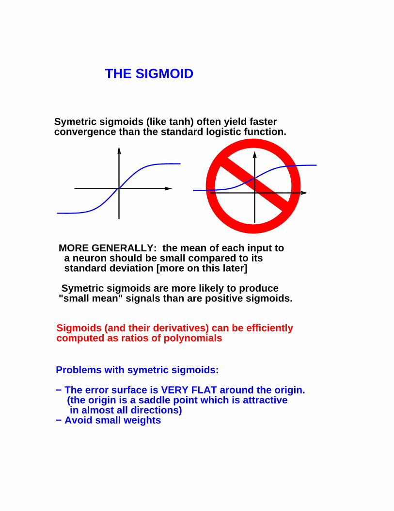
Symetric sigmoids (like tanh) often yield fasterconvergence than the standard logistic function.

MORE GENERALLY: the mean of each input to a neuron should be small compared to its standard deviation [more on this later]

Symetric sigmoids are more likely to produce"small mean" signals than are positive sigmoids.

Sigmoids (and their derivatives) can be efficientlycomputed as ratios of polynomials

Problems with symetric sigmoids:

− The error surface is VERY FLAT around the origin. (the origin is a saddle point which is attractive in almost all directions)− Avoid small weights

23

The one I use: a rational approximation to

f(x) = 1.7159 tanh( x)

1

1

The precise choice of the sigmoid is almost irrevelant,but some choices are more convenient than others

Properties: − f(1) =1, f(−1)=−1 − 2nd derivative is maximum at x=1 − the effective gain is close to 1

THE SIGMOID (continued)

It is sometimes helpful to add a small linear termto avoid flat spots, e.g.

f(x) = tanh(x) + ax

NORMALIZING THE INPUTS

Each input input variable should be sifted sothat its mean (averaged over the training set)is close to 0 (or is small compared to its standard deviation).

Here is why:

Consider the extreme case where the input variablesare always positive.

The weights of neuron in the first hidden layer canonly increase together or decrease together(for a given input pattern the gradients all have the same sign).

This means that if the weight vector has to changeits direction, it will have to do it by zigzaging(read: SLOW).

Shifts of the input variables to a neuron introducea preferred direction for weight changes, whichslows down the learning.

This is also why we prefer symetric sigmoids:what is true for input units is also true for otherunits in the network.

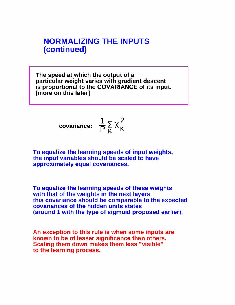
covariance: 1Ρ ∑ χ 2

κ κ

The speed at which the output of a particular weight varies with gradient descent is proportional to the COVARIANCE of its input.[more on this later]

To equalize the learning speeds of input weights, the input variables should be scaled to have approximately equal covariances.

To equalize the learning speeds of these weightswith that of the weights in the next layers,this covariance should be comparable to the expectedcovariances of the hidden units states(around 1 with the type of sigmoid proposed earlier).

An exception to this rule is when some inputs areknown to be of lesser significance than others.Scaling them down makes them less "visible"to the learning process.

NORMALIZING THE INPUTS(continued)

NORMALIZING THE INPUTS(continued)

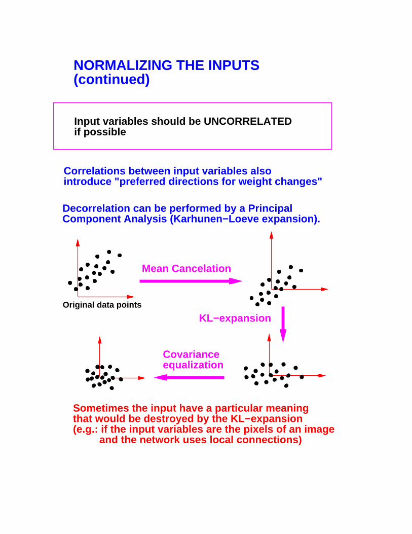
Input variables should be UNCORRELATEDif possible

Correlations between input variables alsointroduce "preferred directions for weight changes"

Sometimes the input have a particular meaningthat would be destroyed by the KL−expansion(e.g.: if the input variables are the pixels of an image and the network uses local connections)

Original data points

Mean Cancelation

KL−expansion

Covarianceequalization

Decorrelation can be performed by a Principal Component Analysis (Karhunen−Loeve expansion).

Avoid saturating the output units. Choosetarget values within the range of the sigmoid

In classification applications, the desiredoutputs are often binary.

Common sense would suggest to set the targetvalues on the asymptotes of the sigmoid.

However this has several adverse effects:

Saturating the units erases the differences betweentypical and non−typical examples.

Setting the target values at the point of maximumsecond derivative on the sigmoid (−1 and +1 for thesigmoid proposed earlier) is the best way to takeadvantage of the non linearity without saturating the units

CHOOSING THE TARGET VALUES

1 − this tends to drive the output weights to infinity (and to saturate the hidden units as well). When a training example happens not to saturate the outputs (say an outlier), it will produce ENORMOUS gradients (due to the large weights).

2 − outputs will tend to be binary EVEN WHEN THEY ARE WRONG. This means that a mistake will be difficult to correct, and that the output levels cannot be used as reliable confidence factors.

INITIALIZING THE WEIGHTS

Initialize the weights so that the expectedstandard deviation of the weighted sumsis at the transition between the linear partand the saturated part of the sigmoid function

Large initial weights saturate the units, leading tosmall gradients and slow learning.Small weights correspond to a very flat area ofthe error surface (especially with symetric sigmoids)

Assuming the sigmoid proposed earlier is used,the expected standard deviation of the inputs toa unit is around 1, and the desired standard deviationof its weighted sum is also around 1.

Assuming the inputs are independent, the expected standard deviation of the weighted sum is

σ = ( ∑ ω ) = φ ϖi

2i

½ ½

where is the number of input to the unit, and is the standard deviation of its incoming weights.

φϖ

ϖ = φ -½

σTo ensure that is close to 1, the weights to a unit can be drawn from a distribution with standard deviation

CHOOSING LEARNING RATES

Equalize the learning speeds.

ηEach weight (or parameter) should have its ownlearning rate. Some weights may require a small learning rateto avoid divergence, while others may requirea large learning rate to converge at reasonable speed.

Because of possible correlations between inputvariables, the learning rate of a unit should beinversely proportional to the square root of thenumber of inputs to the unit.

If shared weights are used (as in TDNNs andconvolutional networks), the learning rate ofa weight should be inversely proportional to thesquare root of the number of connection sharingthat weight.

Learning rates in the lower layers should generallybe larger than that in the higher layers.

The rationale for many of these rules of thumbwill become clearer later.Several techniques are available to reduce"learning rate fiddling".

NEURONS AND WEIGHTS

Although most systems use neurons basedon dot products and sigmoids, many other typesof units (or layers) can be used.

A particularly interesting example is when the dotproduct of the input by the weight vector is replacedby a Euclidean distance, and the sigmoid by anexponential (Gaussian units of RBF).

These units can replace (or coexist with) standardunits, and they can be trained with gradient descent:

ω

Β2

exp

||ω−Ι||

Ι

FPROP

BPROP

Ο = (Ι+Β)exp

δΙ = Ο δΟ ; δΒ = δΙweight vector: FPROP

BPROP

Ο = (ω−Ι)′(ω−Ι)

δΙ = 2 δΟ′(Ι−ω) ; δω = −δΙ

exponential + Bias:

PROS and CONS − Locality: each unit is only affected by a small part of the input space. This can be good (for learning speed) and bad (a lot of RBF are needed to cover high dimensional spaces) − gradient descent learning may fail if the RBFs are not properly initialized (using clustering techniques e.g. K−means). There are LOTS of local minima. − RBFs are more apropriate in higher layers, and sigmoids in lower layers (higher dimension).

MORE STANDARD TRICKS

− Momentum − Increases speed in batch mode. seems marginally useful but not indispensable in stochastic mode.

− Adaptive learning rates: − a separate learning rate for each weight is increased if the gradient is steady, decreased if the gradient changes sign often [Jacobs 88]. This only works with BATCH.

− a global learning rate is adjusted using line searches. Again, this only works for BATCH.

2

THE CONVERGENCE OF

GRADIENT DESCENT

A LITTLE THEORY

weight vector learning rate

gradient ofobjective function

Ε(ω)

ω

Ε(ω)

ω

opt opt

∂Ε∂ωω ← ω − η

Ε(ω)

ω

optη < η

Ε(ω)

ω

η = ηopt

η > η η > 2 η

Gradient Descent in one dimension

OPTIMAL LEARNING RATE IN 1D

Ε(ω)

ω

η = ηopt

ω

∂Ε∂ω

∆ω

∂Ε∂ω

Assuming Eis quadratic:

∂ Ε∂ω

2

2∂Ε∂ω

∆ω =

2∂ Ε

2∂ω=

−1

optη

∂Ε∂ω∆ω = η

Weight change:

OptimalLearningRate

MaximumLearningRate optη= 2 ηmax

CONVERGENCE OF GRADIENT DESCENT

Local quadratic approximation of the cost functionaround a minimum:

Hessianminimum

Ε(ω) ≈ Ε(ϖ) + 1/2(ω−ϖ)′ Η(ϖ) (ω−ϖ)

ϖ0

ϖ1

Hessianeigenvectors

Η =ij ∂ Ε∂ω ∂ω

2

i j

HESSIAN Second derivative matrix

Gradient Descent weight update:

∂Ε∂ω

ω = ω −ηκκ+1 = ω −η Η(ω ) (ω −ϖ)κ κ κ

(ω −ϖ) = (Ι − ηΗ(ω ) )(ω −ϖ) κ+1

κ κ

The Hessian is a symetric NxN matrix

Convergence <===> if the prefactor of theright handside shrinksany vector

Ε(ω) ≈ Ε(ϖ) + 1/2[(ω−ϖ)′Θ′] [ΘΗ(ϖ) Θ′] [Θ(ω−ϖ)]

CONVERGENCE OF GRADIENT DESCENT(continued)

ν0

ν1 Ε(ν) ≈ Ε(0) + 1/2 ν′Λ ν

Let be the rotation matrix that make H diagonal:Θ

Now denote: ν = Θ (ω − ϖ)

The eigenvectorsof a diagonal matrixare the coordinate axes

κ+1 κν = (Ι − η Λ) ν

Θ Η Θ′ = Λ ; Θ′Θ=Ι

Gradient Descent in N dimensions can beviewed as N independent unidimensional Gradient Descents along the eigenvectorsof the Hessian.

Gradient update in the transformed space:

Convergence is obtained for η < 2/ λ maxwhere is the largest eigenvalueof the Hessian

maxλ

CONVERGENCE SPEEDOF GRADIENT DESCENT

The maximum learning rate to ensure convergence is

maxmaxη = 2/ λ

The one that yields the fastest convergencein the direction of highest curvature is

maxoptη = 1/ λ

With this choice, the convergence time willbe determined by the directions of SMALLeigenvalues (they will be the slowest to converge).

The convergence time is proportional to:

min

1η λ >

min λ2λ

max

where is the smallest "non−negligible"eigenvalue

λmin

The convergence time is proportional tothe ratio of the largest eigenvalue to smallest"non−negligible" eigenvalue of the Hessian

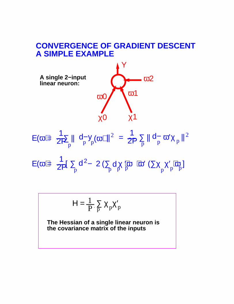
CONVERGENCE OF GRADIENT DESCENTA SIMPLE EXAMPLE

A single 2−input linear neuron:

ω0 ω1

ω2

χ0 χ1

Υ

Η = ∑ χ χ′ pp p 1 P

The Hessian of a single linear neuron isthe covariance matrix of the inputs

Ε(ω) = ∑ || p pp|| 2(ω) pp

2p = ∑ || 1

2P 1 2Pd−y ω′χ || d−

Ε(ω) = [ ∑ − 2 (∑ χ )′ω + ω′ (∑χ χ′ ) ω ]pp pd2 d

p p p 1 2P p

−1.4 −1.2 −1 −0.8 −0.6 −0.4 −0.2 0 0.2 0.4 0.6 0.8 1 1.2 1.4

−1.4

−1.2

−1

−0.8

−0.6

−0.4

−0.2

0

0.2

0.4

0.6

0.8

1

1.2

1.4

Dataset #1

Examples of each class are drawn froma Gaussian distribution centered at(−0.4, −0.8), and (0.4, 0.8).

Eigenvalues of covariance matrix: 0.83 and 0.036

Batch gradient descent

Weight space

−1 −0.8 −0.6 −0.4 −0.2 0 0.2 0.4 0.6 0.8 1

0

0.2

0.4

0.6

0.8

1

1.2

1.4

1.6

1.8

2

Log MSE (dB)

0 1 2 3 4 5 6 7 8 9 10

−20

−15

−10

−5

0

data set: set−1 (100 examples, 2 gaussians)network: 1 linear unit, 2 inputs, 1 output. 2 weights, 1 bias.

Learningrate:

η = 1.5

MaximumadmissibleLearningrate:

Hessianlargesteigenvalue:

λ = 0.84max

η = 2.38max

epochs

Batch gradient descent

Weight space

−1 −0.8 −0.6 −0.4 −0.2 0 0.2 0.4 0.6 0.8 1

0

0.2

0.4

0.6

0.8

1

1.2

1.4

1.6

1.8

2

Log MSE (dB)

0 1 2 3 4 5 6 7 8 9 10

−20

−15

−10

−5

0

data set: set−1 (100 examples, 2 gaussians)network: 1 linear unit, 2 inputs, 1 output. 2 weights, 1 bias.

Learningrate:

MaximumadmissibleLearningrate:

Hessianlargesteigenvalue:

λ = 0.84max

η = 2.38max

epochs

η = 2.5

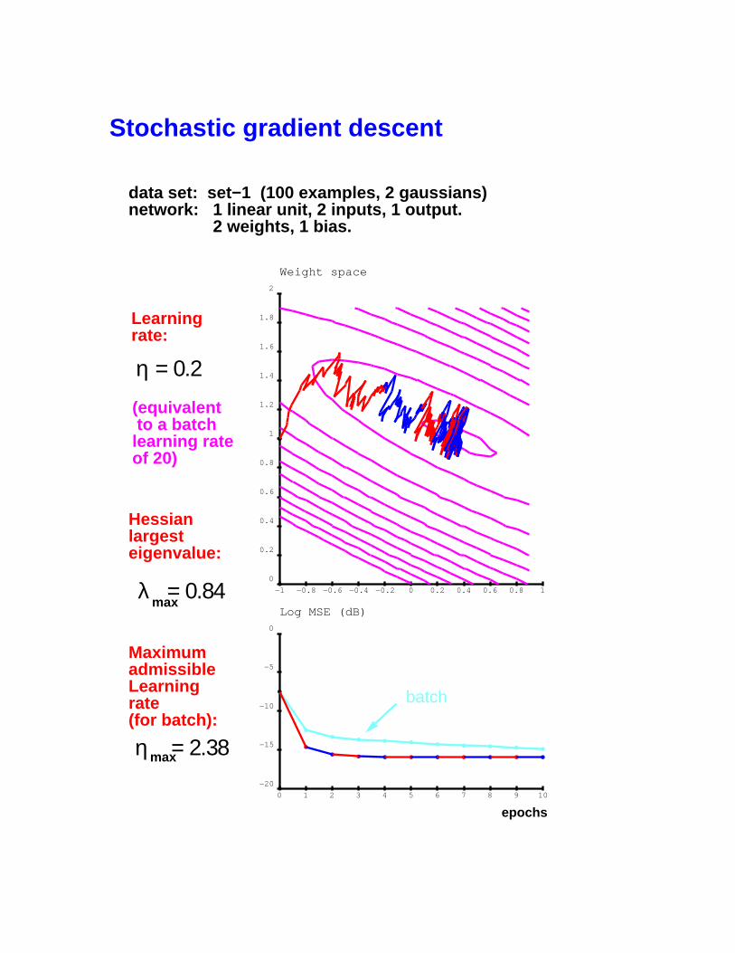
Stochastic gradient descent

data set: set−1 (100 examples, 2 gaussians)network: 1 linear unit, 2 inputs, 1 output. 2 weights, 1 bias.

Learningrate:

Hessianlargesteigenvalue:

λ = 0.84max

η = 2.38max

MaximumadmissibleLearningrate (for batch):

η = 0.2

Weight space

−1 −0.8 −0.6 −0.4 −0.2 0 0.2 0.4 0.6 0.8 1

0

0.2

0.4

0.6

0.8

1

1.2

1.4

1.6

1.8

2

Log MSE (dB)

0 1 2 3 4 5 6 7 8 9 10

−20

−15

−10

−5

0

epochs

batch

(equivalent to a batchlearning rateof 20)

CONVERGENCE OF GRADIENT DESCENT:MINIMAL MULTILAYER NETWORK

1 input1 hidden unit1 output

2 weights2 biases

ω0

ω1ω2

Υ

ω3

χ

TRAINING SET: 20 examples.

Class1: 10 examples drawn from a Gaussian distribution with mean −1, and standard deviation 0.4

Class2: 10 examples drawn from a Gaussian distribution with mean +1, and standard deviation 0.4

Sigmoid: 1.71 tanh(2/3 x)

Targets: −1 for class 1, +1 for class 2

Log MSE (dB)

0 1 2 3 4 5 6 7 8 9 10

−20

−15

−10

−5

0

Weight space

−2 −1.6 −1.2 −0.8 −0.4 0 0.4 0.8 1.2 1.6 2 2.4

−1.4

−1.2

−1

−0.8

−0.6

−0.4

−0.2

0

0.2

0.4

0.6

0.8

1

1.2

1.4

1.6

1.8

2

Learningrate:

epochs

Stochastic gradient: 1−1−1 network

data set: 20 examples, 2 1D−gaussians)network: 1 input, 1 hidden, 1output 2 weights 2biases

η = 0.4

>>

> fi

lena

me

INPUT TRANSFORMATIONSERROR SURFACE TRANSFORMATIONS

A shift (non zero mean) in the input variablescreates a VERY LARGE eigenvalue whichleads to eccentric paraboloids, and to slowconvergence

Subtract the means from the input variables

Normalize the variances of the input variables

Decorrelate the input variables

Correlations between input variables leadto eccentric paraboloid with ROTATED axes

widely spread variances for the input variableslead to widely spread Hessian eigenvalues

The gradient is NOT the best descent directionUse a spearate learning rate for each weight.No use spending time and effort tocompute an accurate gradient estimate

For a single linear neuron, If the input variables have zero means, the eigenvectors of the Hessian are the principal axes of the cloud of training vectors

3

SECOND ORDER METHODS

NEWTON ALGORITHM

Newton Algorithm in one dimension

Ε(ω)

ω

ω

∂Ε∂ω

∆ω

∂Ε∂ω

Assuming Eis quadratic:

∂ Ε∂ω

2

2∂Ε∂ω

∆ω =

Optimal weight change:

2∂ Ε

2∂ω

−1∂Ε∂ω∆ω =

2∂ Ε

2∂ω

−1∂Ε∂ω∆ω = η 0<η<1

If E is not perfectly :quadratic

Hessian

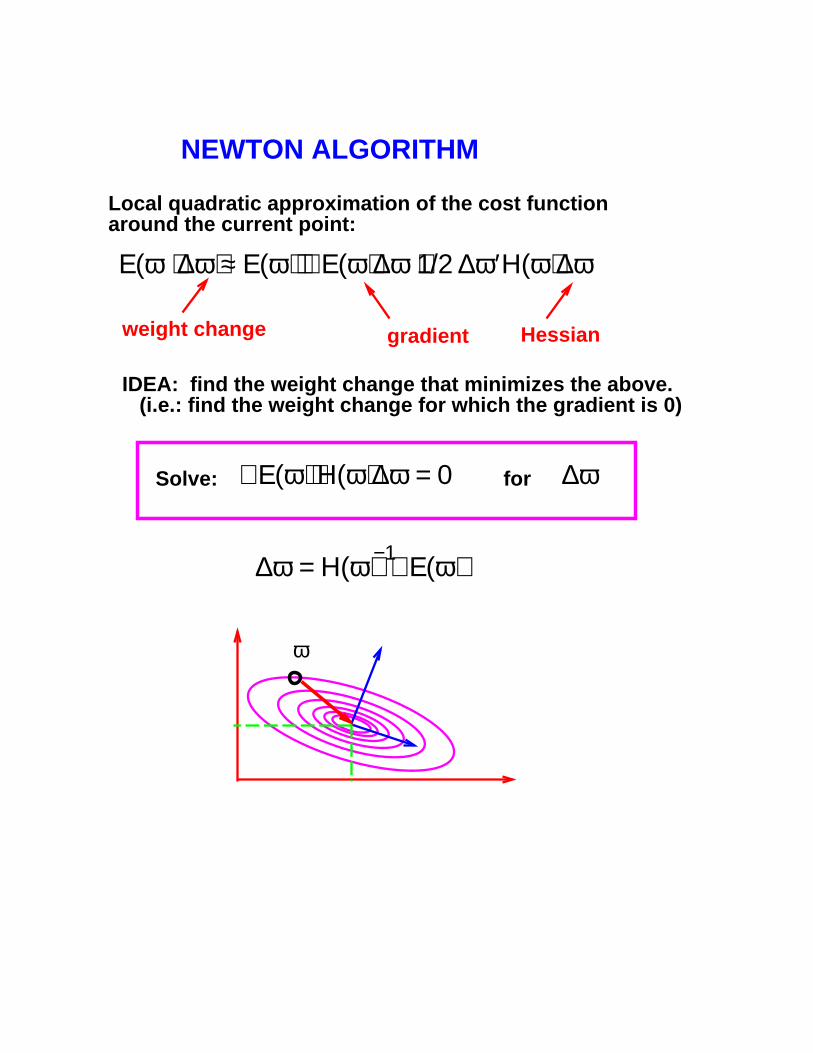
NEWTON ALGORITHM

Local quadratic approximation of the cost functionaround the current point:

Ε(ω + ∆ω) ≈ Ε(ω) + ∇Ε(ω) ∆ω +1/2 ∆ω′Η(ω) ∆ω

gradientweight change

Solve: ∇Ε(ω) + Η(ω) ∆ω = 0 for ∆ω

∆ω = Η(ω) ∇Ε(ω)−1

IDEA: find the weight change that minimizes the above. (i.e.: find the weight change for which the gradient is 0)

ω

½ ½Η(ω)= Θ′Λ Λ Θ

NEWTON ALGORITHM ANDPARAMETER SPACE TRANSFORMS

Η (ω)= ΘΛ Λ Θ′-½ -½-1

ω -½Λ Θ′

-½ΘΛ

U

Network

input

output

ω Networkω

input

output

Θ-½ΛU

Newton Algorithm here ...... ....is like Gradient Descent there

Diagonalized Hessian

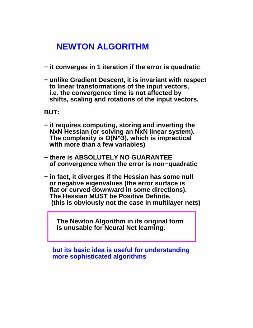
NEWTON ALGORITHM

− it converges in 1 iteration if the error is quadratic

− unlike Gradient Descent, it is invariant with respect to linear transformations of the input vectors, i.e. the convergence time is not affected by shifts, scaling and rotations of the input vectors.

BUT:

− it requires computing, storing and inverting the NxN Hessian (or solving an NxN linear system). The complexity is O(N^3), which is impractical with more than a few variables)

− there is ABSOLUTELY NO GUARANTEE of convergence when the error is non−quadratic

− in fact, it diverges if the Hessian has some null or negative eigenvalues (the error surface is flat or curved downward in some directions). The Hessian MUST be Positive Definite. (this is obviously not the case in multilayer nets)

The Newton Algorithm in its original formis unusable for Neural Net learning.

but its basic idea is useful for understandingmore sophisticated algorithms

COMPUTING THE HESSIANINFORMATION IN MULTILAYER NETWORKS

There are many techniques to compute the fullHessian, or parts of it, or approximations to it,in multilayer networks.

We will review the following simple methods:

− finite difference

− square Jacobian approximation (for the Gauss−Newton and Levenberg−Marquardt algorithms)

− computing the diagonal term (or block diagonal terms) by backpropagation

− computing the product of the Hessian by a vector without computing the Hessian

There exist more complex techniques to computesemi−analytically the full Hessian[Bishop 92, Buntine&Weigend 93, others.....]but they are REALLY complicated, and requiremany forwardprop/backprop passes.

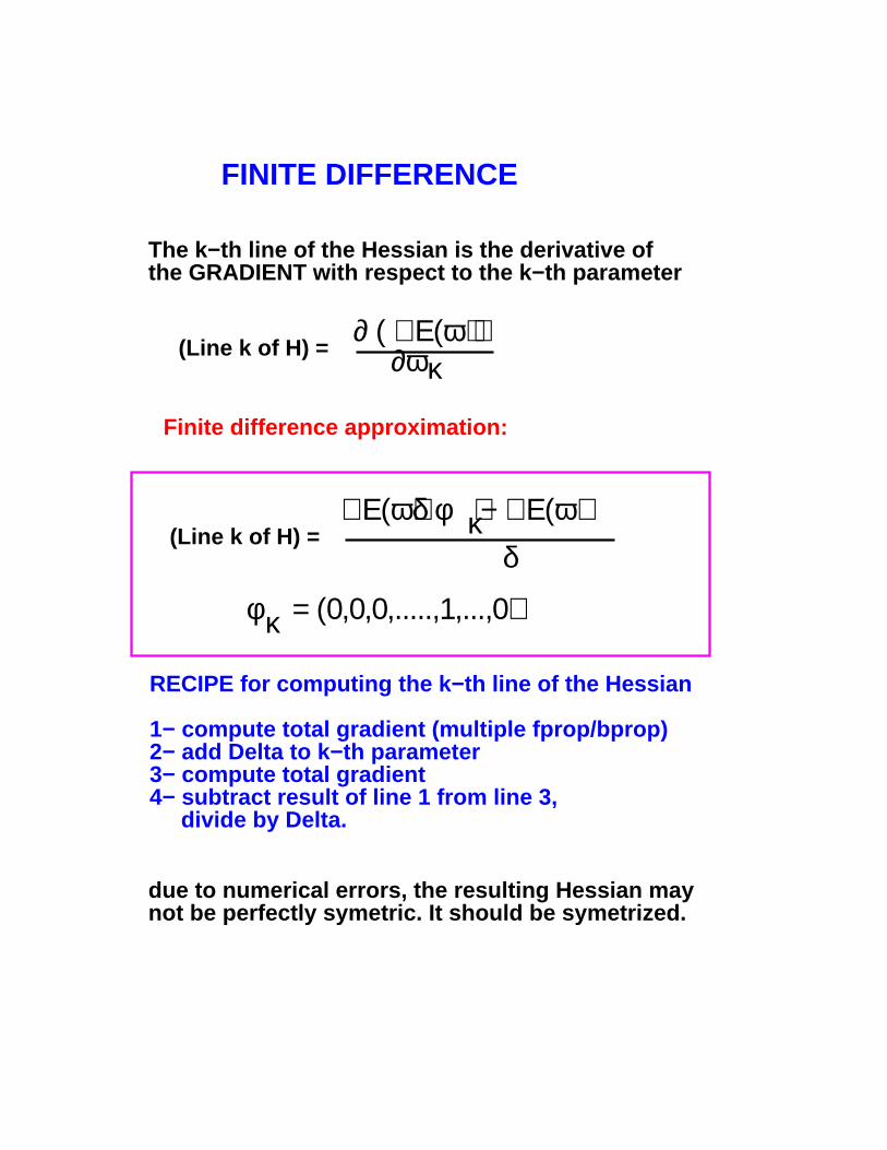
FINITE DIFFERENCE

(Line k of H) =

∂ ( ∇Ε(ω) ) ∂ωκ

Finite difference approximation:

The k−th line of the Hessian is the derivative ofthe GRADIENT with respect to the k−th parameter

RECIPE for computing the k−th line of the Hessian

1− compute total gradient (multiple fprop/bprop)2− add Delta to k−th parameter3− compute total gradient4− subtract result of line 1 from line 3, divide by Delta.

due to numerical errors, the resulting Hessian maynot be perfectly symetric. It should be symetrized.

(Line k of H) =

κδ

∇Ε(ω+δ φ ) − ∇Ε(ω)

κφ = (0,0,0,.....,1,...,0)

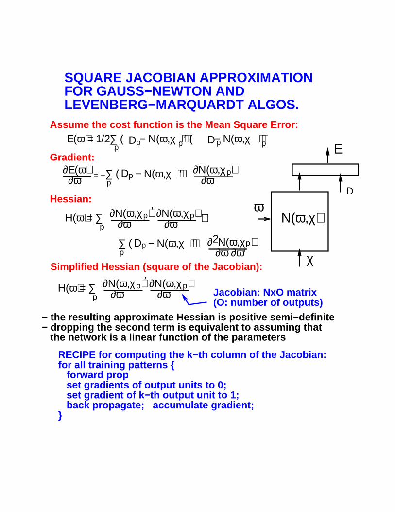
SQUARE JACOBIAN APPROXIMATIONFOR GAUSS−NEWTON ANDLEVENBERG−MARQUARDT ALGOS.

∂Ν(ω,χ ) ∂ω

pDpp∑ ( − Ν(ω,χ ) )′ ∂Ε(ω)

∂ω = −

Gradient:

D D pp ppp

Ε(ω) = 1/2∑ ( − Ν(ω,χ ) )′ ( − Ν(ω,χ ) )Assume the cost function is the Mean Square Error:

p

∂Ν(ω,χ ) ∂ω

pΗ(ω) = ∑ ∂Ν(ω,χ ) ∂ω

p ′+

Dpp∑ ( − Ν(ω,χ ) )′ p∂ Ν(ω,χ )

∂ω ∂ω′2

Hessian:

Simplified Hessian (square of the Jacobian):

ω

χ

Ν(ω,χ)

D

Ε

p

∂Ν(ω,χ ) ∂ω

pΗ(ω) = ∑ ∂Ν(ω,χ ) ∂ω

p ′Jacobian: NxO matrix(O: number of outputs)

RECIPE for computing the k−th column of the Jacobian:for all training patterns { forward prop set gradients of output units to 0; set gradient of k−th output unit to 1; back propagate; accumulate gradient;}

− the resulting approximate Hessian is positive semi−definite− dropping the second term is equivalent to assuming that the network is a linear function of the parameters

ignore this!

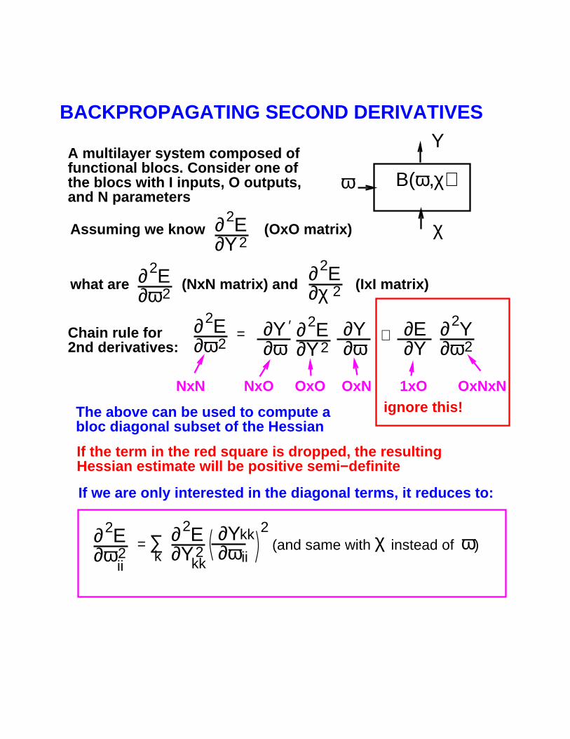
BACKPROPAGATING SECOND DERIVATIVES

ω

Υ

χ

Β(ω,χ)

Assuming we know ∂ Ε∂Υ

2

2

what are 2

2∂ Ε∂ω

2

2∂ Ε∂χ

A multilayer system composed of functional blocs. Consider one of the blocs with I inputs, O outputs, and N parameters

(OxO matrix)

(NxN matrix) and (IxI matrix)

2

2= ∂ Ε

∂Υ2

2∂Υ∂ω

′ ∂Υ∂ω

+ ∂Ε∂Υ

2

2∂ Υ∂ω

∂ Ε∂ω

OxONxO OxNNxN 1xO OxNxN

Chain rule for 2nd derivatives:

The above can be used to compute a bloc diagonal subset of the Hessian

If we are only interested in the diagonal terms, it reduces to:

qIf the term in the red square is dropped, the resultingHessian estimate will be positive semi−definite

(and same with instead of )χ ω=2

2∂ Ε∂ω

ii

∂ Ε∂Υ

2

2∂Υ∂ω

kk

kk

ii∑k

2

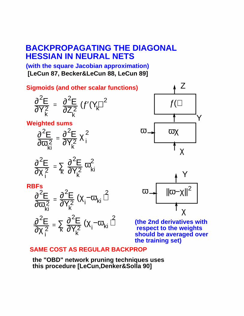
BACKPROPAGATING THE DIAGONALHESSIAN IN NEURAL NETS

ωΥ

χ

ωχ

ƒ()

Ζ

Weighted sums

= ∂ Ε∂Υ

2

2∑k

2

2∂ Ε∂χ

i

2ωki

k

(with the square Jacobian approximation)

RBFs

Sigmoids (and other scalar functions)

∂ Ε∂Ζ

2

2=

2

2∂ Ε∂Υ (ƒ′(Υ))2

k kk

ω

Υ

χ

||ω−χ||2

= ∂ Ε∂Υ

2

2 iχ 2∂ Ε

∂ωki

2

2k

=∂ Ε∂ω

ki

2

2∂ Ε∂Υ

2

2 i

2

kki(χ −ω )

=2

2∂ Ε∂χ

i

∑k

= ∂ Ε∂Υ

2

2 i

2

kki(χ −ω )

[LeCun 87, Becker&LeCun 88, LeCun 89]

the "OBD" network pruning techniques uses this procedure [LeCun,Denker&Solla 90]

(the 2nd derivatives with respect to the weights should be averaged over the training set)

SAME COST AS REGULAR BACKPROP

COMPUTING THE PRODUCT OF THEHESSIAN BY A VECTOR

ω

χ

Ν(ω,χ)

D

Ε

(without computing the Hessian itself)

1α

∂Ε∂ω (ω) −∂Ε

∂ω )(ω+αΨΗΨ≈

Finite difference:

RECIPE for computing the productof a vector by the Hessian:

1− compute gradient2− add to the parameter vector3− compute gradient with perturbed parameters4− subtract result of 1 from 3, divide by

Ψ

αΨ

α

This method can be used to compute the principaleigenvector and eigenvalue of H by the power method.

By iterating Ψ ← ΗΨ / ||Ψ|| Y

||Ψ|| will converge to the principal eigenvector of Hand to the corresponding eigenvalue[LeCun, Simard&Pearlmutter 93]

A more accurate method which does not use finitedifferences (and has the same complexity) has recently been proposed [Pearlmutter 93]

−What does the Hessian of a multilayer network look like?− How does it change with the architecture and the details of the implementation?

− Typically, the distribution of eigenvalues of a multilayer network looks like this:

These large ones are the killers

a few small eigenvalues, a largenumber of medium ones, and a small number of very large ones

They come from:− non−zero mean inputs or neuron states− wide variations second derivatives from layer to layer− correlations between state variables

for more details see [LeCun, Simard&Pearlmutter 93][LeCun, Kanter&Solla 91]

ANALYSIS OF THE HESSIANIN MULTILAYER NETWORKS

EIGENVALUE SPECTRUM

Network: 256−128−64−10 with local connections and shared weights (around 750 parameters) Data set: 320 handwritten digits

0 100 200 300 400 500 600 700 800−6

−5.5

−5

−4.5

−4

−3.5

−3

−2.5

−2

−1.5

−1

−0.5

0

Eigenvalue order

10Lo

g

Eig

enva

lue

the ratio between the 1st and the 11th eigenvalues is 8

0 2 4 6 8 10 12 14 1601234567891011121314151617181920

Eigenvalue magnitude

Number of Eigenvalues

Big killers

HISTOGRAM

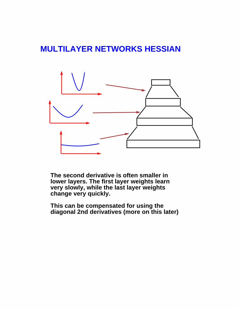
MULTILAYER NETWORKS HESSIAN

The second derivative is often smaller inlower layers. The first layer weights learnvery slowly, while the last layer weights change very quickly.

This can be compensated for using thediagonal 2nd derivatives (more on this later)

CLASSICAL 2ND ORDEROPTIMIZATION METHODS

− Conjugate Gradient methods − O(N) methods − do not use the Hessian directly − attempts to find descent directions that minimally disturb the result of the previous iterations − uses line search. Works only in BATCH.

− Gauss−Newton and Levenberg−Marquardt methods − use the square Jacobian approximation − works only for mean−square error − mainly designed for BATCH − O(N^3)

− Quasi−Newton methods (BFGS) − iteratively computes an estimate of the inverse Hessian. − requires a line search. Works only in BATCH. − O(N^2)

[Dennis&Schnabel 83], [Fletcher 87], [Press et al. 88] [Battiti 92]

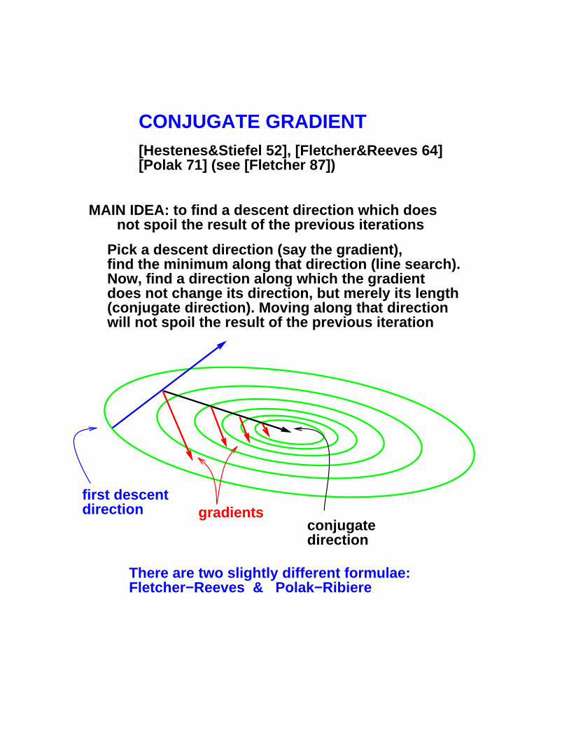
CONJUGATE GRADIENT[Hestenes&Stiefel 52], [Fletcher&Reeves 64][Polak 71] (see [Fletcher 87])

Pick a descent direction (say the gradient),find the minimum along that direction (line search).Now, find a direction along which the gradientdoes not change its direction, but merely its length(conjugate direction). Moving along that directionwill not spoil the result of the previous iteration

MAIN IDEA: to find a descent direction which does not spoil the result of the previous iterations

first descentdirection gradients

conjugatedirection

There are two slightly different formulae:Fletcher−Reeves & Polak−Ribiere

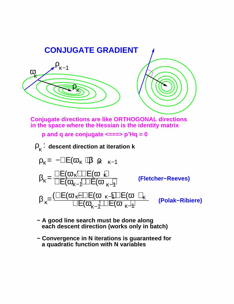
CONJUGATE GRADIENT

Conjugate directions are like ORTHOGONAL directionsin the space where the Hessian is the identity matrix

p and q are conjugate <===> p’Hq = 0

descent direction at iteration k

ρ = −∇Ε(ω ) + β ρκ κ κ κ−1

ρ κ−1

ρ κ

κω

β =κ∇Ε(ω )′ ∇Ε(ω )∇Ε(ω )′ ∇Ε(ω )

κκκ−1κ−1

(Fletcher−Reeves)

(∇Ε(ω )−∇Ε(ω ))′ ∇Ε(ω ) ∇Ε(ω )′ ∇Ε(ω )β =κ κ−1κ−1

κ κ−1 κ (Polak−Ribiere)

κρ :

− A good line search must be done along each descent direction (works only in batch)

− Convergence in N iterations is guaranteed for a quadratic function with N variables

CONJUGATE GRADIENT

− Conjugate gradient is simple and effective. the Polak−Ribiere formula seems to be more robust for non−quadratic functions.

− The conjugate gradient formulae can be viewed as "smart ways" to choose the momentum.

− Conjugate gradient has been used with success in the context of multilayer network training [Kramer&Sangiovani−Vincentelli 88, Barnard&Cole 88, Bengio&Moore 89, Møller 92, Hinton’s group in Toronto.....]

− It seems particularly apropriate for moderate size problems with relatively low redundancy in the data. Typical applications include function approximation, robotic control, times−series prediction, and other real−valued problems (especially if a high accuracy solution is sought). On large classification problems, stochastic backprop is faster.

− The main drawback of CG is that it is a BATCH method, partly due to its requirement for an accurate line search. There have been attempts to solve that problem using "mini−batches" [Møller 92].

BFGS and Quasi−Newton methods

ρ = Μ ∇Ε(ω)ρ ω ← ω − ηρ

There exist several Quasi−Newton methods,but the most successful is theBroyden−Fletcher−Goldfarb−Shanno (BFGS)method.

[Fletcher 87],[Dennis&Schnabel 83], [Watrous 88],[Battiti 92].

Compared to Newton method, Quasi−Newtonmethods only require the first derivative, theyuse positive definite approximations to the inverse Hessian (which means they go downhill), and they require O(N^2) operations per iteration.

All of the quasi−Newton methods are BATCH methods

Quasi−Newton (or secant) methods attempt tokeep a positive definite estimate of the INVERSE HESSIAN directly, without requiring matrix inversion, and by only resorting to the gradient information.

They work as follows:

1− pick a positive definite matrix M (say M=I)2− set search direction3− line search along giving 4− update estimate of inverse Hessian M

BFGS

past parameter vector:present parameter vector:past parameter increment:past gradient:present gradient:past gradient increment:present inverse Hessian:future inverse Hessian

ωωδ = ω − ω∇Ε(ω )∇Ε(ω )ϕ = ∇Ε(ω )−∇Ε(ω )ΜΜ κ

κ−1κ

κ

κκ−1

κ−1

κ−1

κ−1

Μ = Μ + (1+ ϕ′Μϕ δ′ϕ

δδ′δ′ϕ

δϕ′Μ+Μϕδ δϕ) − ( )κ κ−1

ρ = Μ ∇Ε(ω )κκ+1 κ

ω = ω − η ρκκ+1 κ+1 κ+1

update inverse Hessian estimate

compute descent direction

line search

− it is an O(N^2) algorithm BUT− it requires storing an NxN matrix− it is a BATCH algorithm (requires a line search)

Only practical for VERY SMALL networks withnon−redundant training sets.

Several variations exist that attempt to reduce the storage requirements:− limited storage BFGS [Nocedal 80]− memoryless BFGS, OSS [Battiti 92]

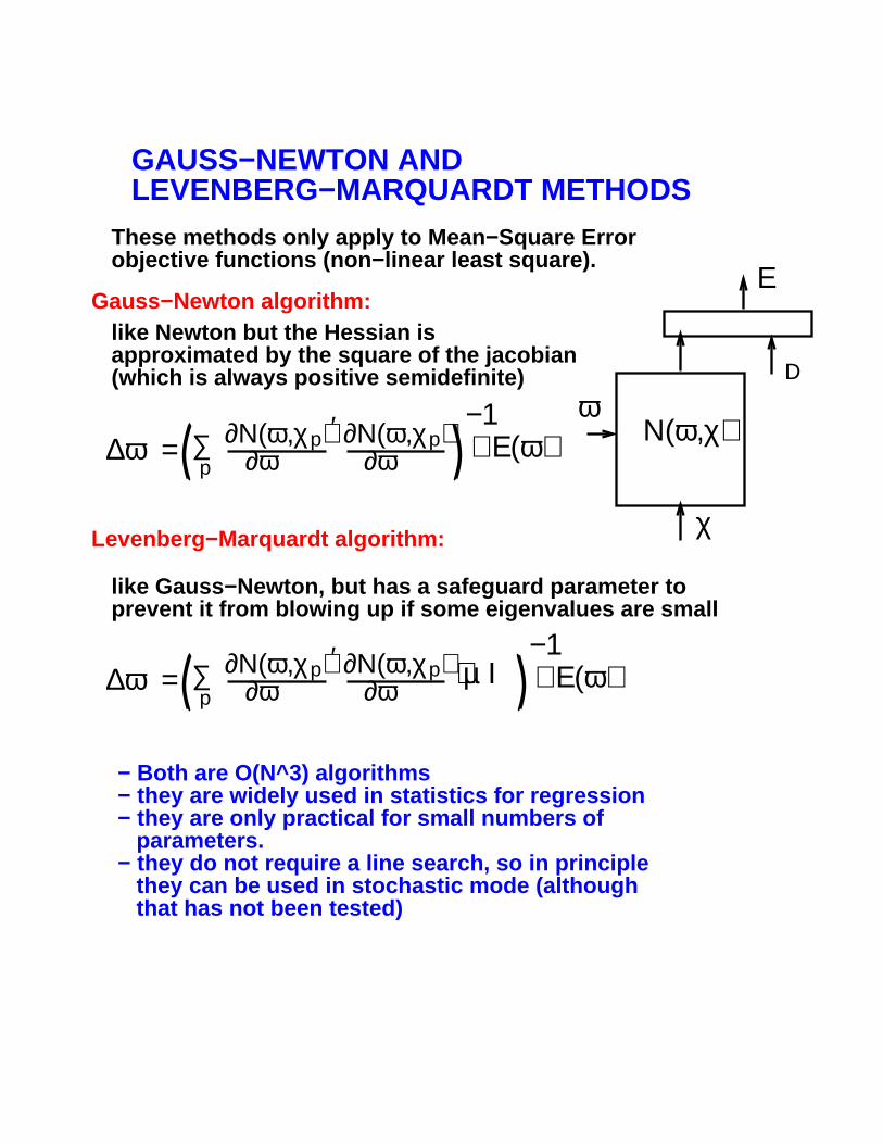
GAUSS−NEWTON ANDLEVENBERG−MARQUARDT METHODS

These methods only apply to Mean−Square Errorobjective functions (non−linear least square).

Gauss−Newton algorithm:

Levenberg−Marquardt algorithm:

ω

χ

Ν(ω,χ)

D

Ε

like Newton but the Hessian is approximated by the square of the jacobian(which is always positive semidefinite)

∆ω = p

∂Ν(ω,χ ) ∂ω

p∂Ν(ω,χ ) ∂ω

p ′∑

−1∇Ε(ω)

like Gauss−Newton, but has a safeguard parameter toprevent it from blowing up if some eigenvalues are small

∆ω = p

∂Ν(ω,χ ) ∂ω

p∂Ν(ω,χ ) ∂ω

p ′∑

−1∇Ε(ω)+ µ Ι

− Both are O(N^3) algorithms − they are widely used in statistics for regression− they are only practical for small numbers of parameters.− they do not require a line search, so in principle they can be used in stochastic mode (although that has not been tested)

4

APPLYING SECOND ORDER

METHODS TO MULTILAYER NETS

(NON)APPLICABILITY OF2nd ORDER METHODS TONEURAL−NET LEARNING

BAD NEWS:

− Full Hessian techniques (GN, LM, BFGS) can only apply to small networks. But small networks are not the ones we need to speed up most.

− Most 2nd order techniques (CG, BFGS....) require a line search, and therefore are not directly usable in stochastic mode

− Many heuristic tricks (adaptive learning rates....) also apply to batch only.

On large classification problems, a carfully tuned stochastic gradient is hard to beat.

On smaller problems requiring accurate real−valuedoutputs (function approximation, control...), conjugate gradient (with Polak−Ribiere) offers the best combination of speed, reliability and simplicity.

This section is devoted to 2nd order techniquesspecifically designed for large neural−net training

MINI BATCH METHODS

Attempts at applying Conjugate Gradient to largeand redundant problems have been made[Kramer&Sangiovani−Vincentelli 88], [Møller 92]

They use "mini batches": subsets of increasingsizes are used.

Møller proposes a systematic way of choosingthe size of the mini batch.

He also uses a variant of CG which he calls"scaled CG". Essentially, the line search is replacedby a 1D Levenberg−Marquardt−like algorithm.

A STOCHASTIC DIAGONALLEVENBERG−MARQUARDTMETHOD

[LeCun 87, Becker&LeCun 88, LeCun 89]

THE MAIN IDEAS:

− use formulae for the backpropagation of the diagonal Hessian (shown earlier) to keep a running estimate of the second derivative of the error with respect to each parameter.

− use these term in a "Levenberg−Marquardt" formula to scale each parameter’s learning rate

∂ Ε∂ω

ki

2

2

Each parameter (weight) has its own learning rate computed as:kiη kiω

ε is a global "learning rate"

µ

is an estimate of thediagonal second derivativewith respect to weight (ki)

kiη

kiη = ε∂ Ε∂ω

ki

2

2+ µ

is a "Levenberg−Marquardt"parameter to prevent form blowing up if the 2ndderivative is small

The second derivatives can be computed using

a running average formula over a subset of the trainingset prior to training:

A STOCHASTIC DIAGONALLEVENBERG−MARQUARDTMETHOD

∂ Ε∂ω

ki

2

2

∂ Ε∂ω

ki

2

2∂ Ε∂ω

ki

2

2+ γ ← (1−γ) ∂ Ε

∂ωki

2

2p

new estimateof 2nd der.

previousestimate

small constant

instantaneous2nd der. forpattern p

The instantaneous second derivatives are computed usingthe formula in the slide entitled:"BACKPROPAGATING THE DIAGONAL HESSIAN IN NEURAL NETS"

Since the second derivatives evolve slowly, there is no needto reestimate them often. They can be estimated once at the beginning by sweeping over a few hundred patterns.Then, they can be reestimated every few epochs.

The additional cost over regular backprop is negligible.

Is usually about 3 times faster than carefully tuned stochastic gradient.

Stochastic Diagonal Levenberg−Marquardt

Weight space

−1 −0.8 −0.6 −0.4 −0.2 0 0.2 0.4 0.6 0.8 1

0

0.2

0.4

0.6

0.8

1

1.2

1.4

1.6

1.8

2

Log MSE (dB)

0 1 2 3 4 5 6 7 8 9 10

−20

−15

−10

−5

0

data set: set−1 (100 examples, 2 gaussians)network: 1 linear unit, 2 inputs, 1 output. 2 weights, 1 bias.

Hessianlargesteigenvalue:

λ = 0.84max

η = 2.38max

epochs

Learningrates:

η0 = 0.12η1 = 0.03η2 = 0.02

MaximumadmissibleLearningrate (batch):

Stochastic Diagonal Levenberg−Marquardt

Weight space

−1 −0.8 −0.6 −0.4 −0.2 0 0.2 0.4 0.6 0.8 1

0

0.2

0.4

0.6

0.8

1

1.2

1.4

1.6

1.8

2

Log MSE (dB)

0 1 2 3 4 5 6 7 8 9 10

−20

−15

−10

−5

0

data set: set−1 (100 examples, 2 gaussians)network: 1 linear unit, 2 inputs, 1 output. 2 weights, 1 bias.

Hessianlargesteigenvalue:

λ = 0.84max

η = 2.38max

epochs

Learningrates:

MaximumadmissibleLearningrate (batch):

η0 = 0.76η1 = 0.18η2 = 0.12

IDEA #1 (the power method):

Ψ ← Η Ψ||Ψ||

HESSIANNEW ESTIMATEOF EIGENVECTOR

OLD ESTIMATEOF EIGENVECTOR

ESTIMATE OFEIGENVALUE

Ψ1 − Choose a vector at random

2 − iterate:

Ψ will converge to the principal eigenvector(or a vector in the principal eigenspace)

||Ψ|| will converge to the correspondingeigenvalue

without computing the Hessian

COMPUTING THE PRINCIPALEIGENVALUE/VECTOR OF THEHESSIAN

NEW ESTIMATEOF EIGENVECTOR

OLD ESTIMATEOF EIGENVECTOR

Η ΨCOMPUTING THE PRODUCT

IDEA #2 (Taylor expansion):

1αΨ ← ∂Ε

∂ω (ω) −∂Ε∂ω ||Ψ||

Ψ(ω+α )

GRADIENTPERTURBEDGRADIENT

"SMALL"CONSTANT

One iteration of this procedure requires2 forward props and 2 backward propsfor each pattern in the training set.

This converges very quickly to a goodestimate of the largest eigenvalue of H

NEW ESTIMATEOF EIGENVECTOR

OLD ESTIMATEOF EIGENVECTOR

IDEA #3 (running average):

"SMALL"CONSTANTS

PERTURBEDGRADIENT FORCURRENT PATTERN

GRADIENT FORCURRENTPATTERN

1α

∂Ε∂ω (ω) −∂Ε

∂ω ||Ψ||Ψ(ω+α )Ψ ← (1−γ)Ψ+γ

p p

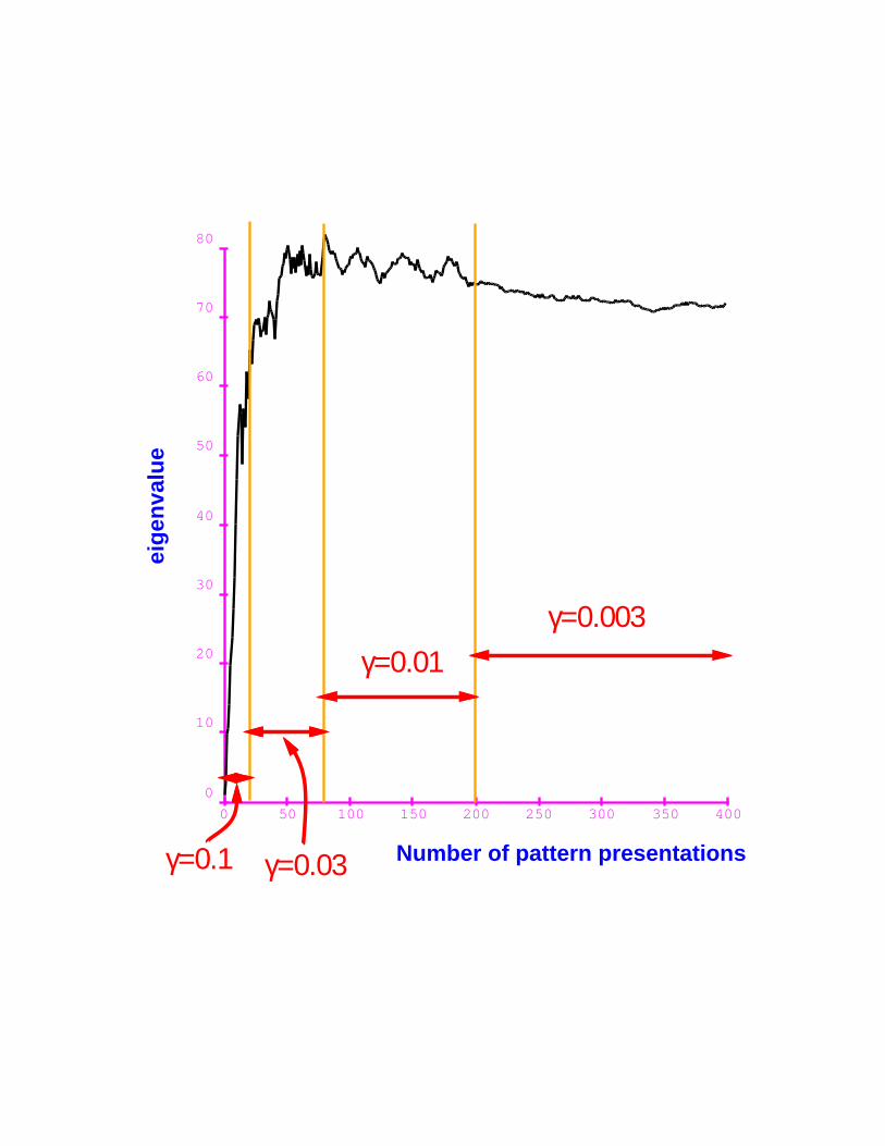
ON−LINE COMPUTATION OF Ψ

This procedure converges VERY quickly to the largesteigenvalue of the AVERAGE Hessian.

The properties of the average Hessian determine thebehavior of ON−LINE gradient descent (stochastic, or per−sample update).

EXPERIMENT: A shared−weight network with 5 layersof weights, 64638 connections and 1278 free parameters.Training set: 1000 handwritten digits.

Correct order of magnitude is obtained in less than100 pattern presentations (10% of training set size)

The fluctuations of the average Hessian over the trainingset are small.

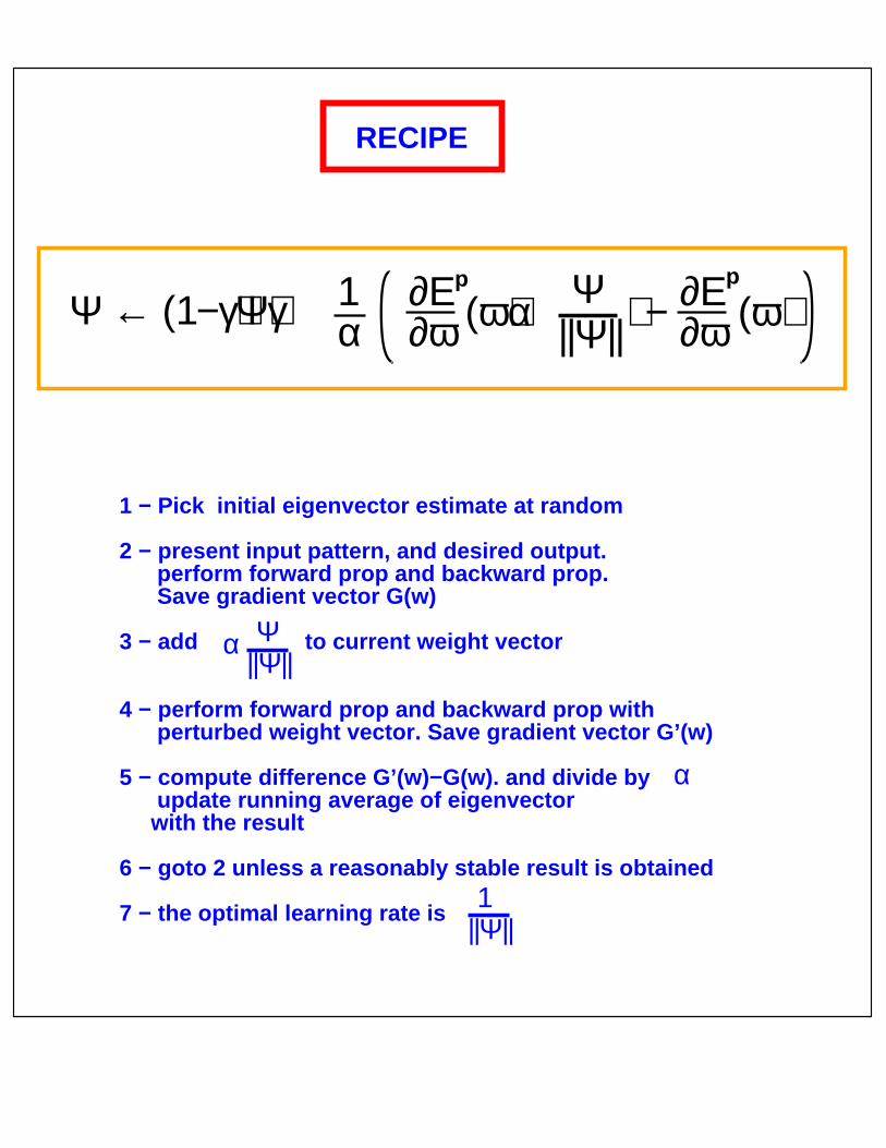
RECIPE

1α

∂Ε∂ω (ω) −∂Ε

∂ω ||Ψ||Ψ(ω+α )Ψ ← (1−γ)Ψ+γ

p p

||Ψ||Ψα

α

||Ψ||1

1 − Pick initial eigenvector estimate at random

2 − present input pattern, and desired output. perform forward prop and backward prop. Save gradient vector G(w)

3 − add to current weight vector

4 − perform forward prop and backward prop with perturbed weight vector. Save gradient vector G’(w)

5 − compute difference G’(w)−G(w). and divide by update running average of eigenvector with the result

6 − goto 2 unless a reasonably stable result is obtained

7 − the optimal learning rate is

0 50 100 150 200 250 300 350 400

0

10

20

30

40

50

60

70

80

Number of pattern presentations

eig

enva

lue

γ=0.1 γ=0.03

γ=0.01γ=0.003

0 0.250.50.75 1 1.251.51.75 2 2.252.52.75 3 3.253.53.75 4

0

0.5

1

1.5

2

2.5

LEARNING RATEPREDICTED OPTIMAL LEARNING RATE

ME

AN

SQ

UA

RE

D E

RR

OR

1 epoch

2 epochs

3 epochs4 epochs

5 epochs

Network: 784x30x10 fully connectedTraining set: 300 handwritten digits

0 0.25 0.5 0.75 1 1.25 1.5 1.75 2 2.25 2.5 2.75 3

0

0.5

1

1.5

2

2.5

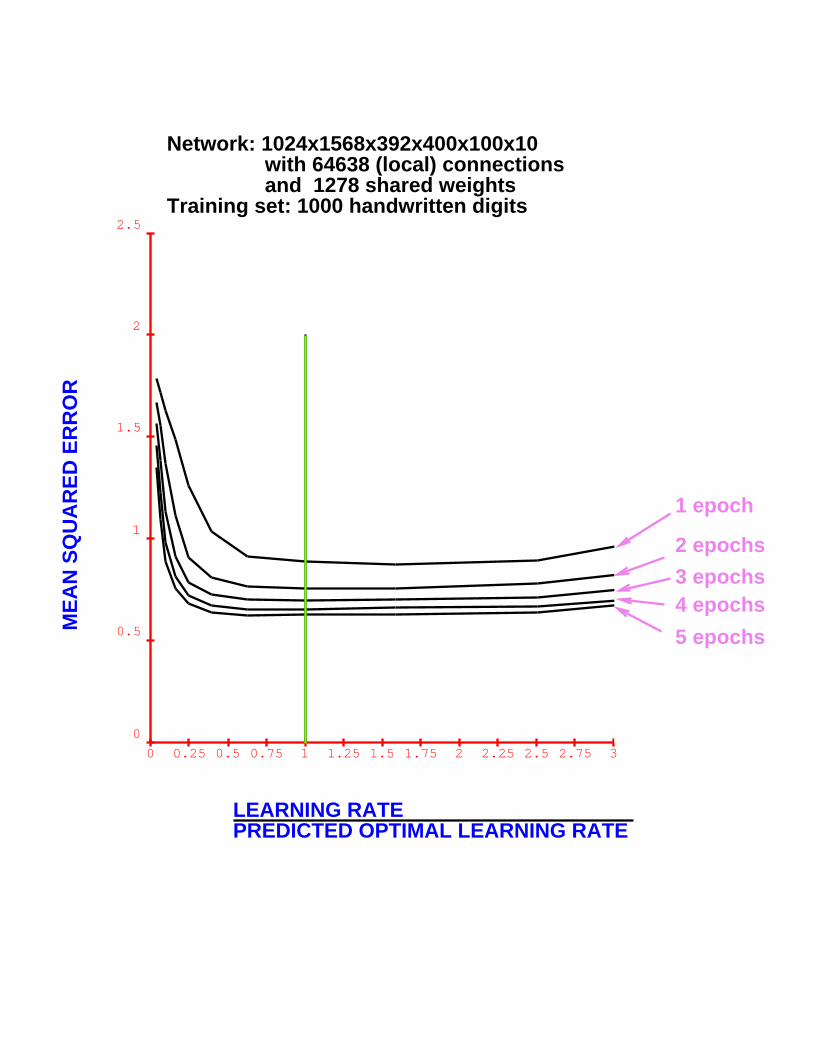
LEARNING RATEPREDICTED OPTIMAL LEARNING RATE

ME

AN

SQ

UA

RE

D E

RR

OR

1 epoch

2 epochs

3 epochs4 epochs

5 epochs

Network: 1024x1568x392x400x100x10 with 64638 (local) connections and 1278 shared weightsTraining set: 1000 handwritten digits