efficient methods for structural …...ii efficient methods for structural analysis of built-up...
TRANSCRIPT

EFFICIENT METHODS FOR STRUCTURAL ANALYSIS OF BUILT-UP WINGS
by
Youhua Liu
Dissertation Submitted to the Faculty of Virginia Polytechnic Institute and State University
in partial fulfillment of the requirements for the degree of
DOCTOR OF PHILOSOPHY
In
Aerospace Engineering
Approved:
Rakesh K. Kapania, Chairman
Romesh C. Batra Zafer Gürdal
Eric R. Johnson Efstratios Nikolaidis
April 2000Blacksburg, Virginia
Keywords: Built-Up Wing, Structural Analysis, Continuum Model, Equivalent Plate Model,Mindlin-Plate Theory, Ritz-Method, Neural Network, Sensitivity
Copyright ¶ 2000, Youhua Liu

ii
Efficient Methods for Structural Analysis of Built-Up Wings
by
Youhua Liu
Committee Chairman: Rakesh K. Kapania
Aerospace and Ocean Engineering
(ABSTRACT)
The aerospace industry is increasingly coming to the conclusion that physics-based high-
fidelity models need to be used as early as possible in the design of its products. At the preliminary
design stage of wing structures, though highly desirable for its high accuracy, a detailed finite
element analysis(FEA) is often not feasible due to the prohibitive preparation time for the FE
model data and high computation cost caused by large degrees of freedom. In view of this situation,
often equivalent beam models are used for the purpose of obtaining global solutions. However, for
wings with low aspect ratio, the use of equivalent beam models is questionable, and using an
equivalent plate model would be more promising.
An efficient method, Equivalent Plate Analysis or simply EPA, using an equivalent plate
model, is developed in the present work for studying the static and free-vibration problems of built-
up wing structures composed of skins, spars, and ribs. The model includes the transverse shear
effects by treating the built-up wing as a plate following the Reissner-Mindlin theory (FSDT). The
Ritz method is used with the Legendre polynomials being employed as the trial functions.
Formulations are such that there is no limitation on the wing thickness distribution. This method is
evaluated, by comparing the results with those obtained using MSC/NASTRAN, for a set of
examples including both static and dynamic problems.

iii
The Equivalent Plate Analysis (EPA) as explained above is also used as a basis for generating
other efficient methods for the early design stage of wing structures, such that they can be
incorporated with optimization tools into the process of searching for an optimal design. In the
search for an optimal design, it is essential to assess the structural responses quickly at any design
space point. For such purpose, the FEA or even the above EPA, which establishes the stiffness and
mass matrices by integrating contributions spar by spar, rib by rib, are not efficient enough.
One approach is to use the Artificial Neural Network (ANN), or simply called Neural Network
(NN) as a means of simulating the structural responses of wings. Upon an investigation of
applications of NN in structural engineering, methods of using NN for the present purpose are
explored in two directions, i.e. the direct application and the indirect application. The direct method
uses FEA or EPA generated results directly as the output. In the indirect method, the wing inner-
structure is combined with the skins to form an "equivalent" material. The constitutive matrix,
which relates the stress vector to the strain vector, and the density of the equivalent material are
obtained by enforcing mass and stiffness matrix equities with regard to the EPA in a least-square
sense. Neural networks for these material properties are trained in terms of the design variables of
the wing structure. It is shown that this EPA with indirect application of Neural Networks, or
simply called an Equivalent Skin Analysis (ESA) of the wing structure, is more efficient than the
EPA and still fairly good results can be obtained.
Another approach is to use the sensitivity techniques. Sensitivity techniques are frequently used
in structural design practices for searching the optimal solutions near a baseline design. In the
present work, the modal response of general trapezoidal wing structures is approximated using
shape sensitivities up to the second order, and the use of second order sensitivities proved to be
yielding much better results than the case where only first order sensitivities are used. Also
different approaches of computing the derivatives are investigated. In a design space with a lot of
design points, when sensitivities at each design point are obtained, it is shown that the global
variation in the design space can be readily given based on these sensitivities.

v
Acknowledgments
This work would not have been accomplished without the support and guidance of my advisor
and committee chairman, Dr. Rakesh K. Kapania. Dr. Kapania's professional attitude influenced me
a lot, and his prompt responses to my questions and submitted work, encouragement during all
phases of my work, and his understanding are greatly appreciated. I am grateful to Dr. Romesh C.
Batra, Dr. Zafer Gürdal, Dr. Eric R. Johnson, and Dr. Efstratios Nikolaidis for serving in my
committee. I would like to thank the financial support of NASA Langley Research Center on this
research through Grant NAG-1-1884 with Dr. Jerry Housner and Dr. John Wang as the Technical
Monitors. I am also thankful to other students for the helps I have received, especially Dr. Daniel
Hammerand, Dr. Luohui Long, and Mr. Erwin Sulaeman.
Finally, I would say this work could not have got started, let alone been finished, without the
unconditional support, trust and love of my wife, Ting, and my daughter, Lisa. I owe them a lot.
vi
Contents
List of Tables x
List of Figures xi
Nomenclature xvi
1. Introduction 1
1.1 The Trend of Early Analysis in Product Design. . . . . . . . . . . . . . . . . . . . . . . . . . . . . . . 1
1.2 Neural Networks. . . . . . . . . . . . . . . . . . . . . . . . . . . . . . . . . . . . . . . . . . . . . . . . . . . . . . . 3
1.2.1 History and Concepts. . . . . . . . . . . . . . . . . . . . . . . . . . . . . . . . . . . . . . . . . . . . 3
1.2.2 Applications in Structural Engineering. . . . . . . . . . . . . . . . . . . . . . . . . . . . . . 4
1.3 Continuum Models. . . . . . . . . . . . . . . . . . . . . . . . . . . . . . . . . . . . . . . . . . . . . . . . . . . . . 5
1.4 Plate Theories. . . . . . . . . . . . . . . . . . . . . . . . . . . . . . . . . . . . . . . . . . . . . . . . . . . . . . . . . 6
1.5 Sensitivity Techniques. . . . . . . . . . . . . . . . . . . . . . . . . . . . . . . . . . . . . . . . . . . . . . . . . . .8
1.6 Scope of the Present Work. . . . . . . . . . . . . . . . . . . . . . . . . . . . . . . . . . . . . . . . . . . . . . . 8
2. Neural Networks and Its Applications 11
2.1 Two Important Types of NN. . . . . . . . . . . . . . . . . . . . . . . . . . . . . . . . . . . . . . . . . . . . .11
2.1.1 Feed-Forward Multi-Layer Neural Network. . . . . . . . . . . . . . . . . . . . . . . . . 12
2.1.2 Radial Basis Function Neural Network. . . . . . . . . . . . . . . . . . . . . . . . . . . . . 15
2.2 Features of ANN. . . . . . . . . . . . . . . . . . . . . . . . . . . . . . . . . . . . . . . . . . . . . . . . . . . . . . 16
2.3 Algorithms in the MATLAB Neural Network Toolbox. . . . . . . . . . . . . . . . . . . . . . . . 17
2.4 Ways of Application of Neural Networks. . . . . . . . . . . . . . . . . . . . . . . . . . . . . . . . . . .19
2.4.1 Direct Application. . . . . . . . . . . . . . . . . . . . . . . . . . . . . . . . . . . . . . . . . . . . . 19

vii
2.4.2 Indirect Application. . . . . . . . . . . . . . . . . . . . . . . . . . . . . . . . . . . . . . . . . . . . 20
3. Continuum Model Approaches 21
3.1 Methods of Obtaining Continuum Models. . . . . . . . . . . . . . . . . . . . . . . . . . . . . . . . . . 21
3.2 An Example of NN Modeling of Continuum Models. . . . . . . . . . . . . . . . . . . . . . . . . .23
3.2.1 Neural Network with 2 Input Variables. . . . . . . . . . . . . . . . . . . . . . . . . . . . . .24
3.2.2 Neural Network with 3 Input Variables. . . . . . . . . . . . . . . . . . . . . . . . . . . . . .29
3.2.3 Neural Network with 4 Input Variables. . . . . . . . . . . . . . . . . . . . . . . . . . . . . .29
4. An Approach for the Solution of Mindlin Plates 32
4.1 Assumptions and Formulations. . . . . . . . . . . . . . . . . . . . . . . . . . . . . . . . . . . . . . . . . . .32
4.2 Strain Energy and Stiffness Matrix. . . . . . . . . . . . . . . . . . . . . . . . . . . . . . . . . . . . . . . . 37
4.3 Kinetic Energy and Mass Matrix. . . . . . . . . . . . . . . . . . . . . . . . . . . . . . . . . . . . . . . . . .40
5. Equivalent Plate Analysis of Built-Up Wing Structures 42
5.1 Numerical Integration of Stiffness and Mass Matrices. . . . . . . . . . . . . . . . . . . . . . . . .42
5.1.1 Skins. . . . . . . . . . . . . . . . . . . . . . . . . . . . . . . . . . . . . . . . . . . . . . . . . . . . . . . .43
5.1.2 Spars. . . . . . . . . . . . . . . . . . . . . . . . . . . . . . . . . . . . . . . . . . . . . . . . . . . . . . . .44
5.1.3 Ribs. . . . . . . . . . . . . . . . . . . . . . . . . . . . . . . . . . . . . . . . . . . . . . . . . . . . . . . . .45
5.2 Boundary Conditions. . . . . . . . . . . . . . . . . . . . . . . . . . . . . . . . . . . . . . . . . . . . . . . . . . .46
5.3 Formulation for Vibration Problem of Wing. . . . . . . . . . . . . . . . . . . . . . . . . . . . . . . . .50
5.4 Convergence Test. . . . . . . . . . . . . . . . . . . . . . . . . . . . . . . . . . . . . . . . . . . . . . . . . . . . . 50
5.5 Static Problem Solutions. . . . . . . . . . . . . . . . . . . . . . . . . . . . . . . . . . . . . . . . . . . . . . . . 54
5.6 Results and Discussion. . . . . . . . . . . . . . . . . . . . . . . . . . . . . . . . . . . . . . . . . . . . . . . . . 55
5.6.1 Free Vibration Analysis. . . . . . . . . . . . . . . . . . . . . . . . . . . . . . . . . . . . . . . . . 55
5.6.1.1 A Trapezoidal Plate. . . . . . . . . . . . . . . . . . . . . . . . . . . . . . . . . . . . .55
5.6.1.2 A Trapezoidal Shell with a Camber. . . . . . . . . . . . . . . . . . . . . . . . .57
5.6.1.3 A Solid Wing. . . . . . . . . . . . . . . . . . . . . . . . . . . . . . . . . . . . . . . . . .59
5.6.1.4 A Built-up Wing Composed of Skins, Spars and Ribs. . . . . . . . . . 61
5.6.1.5 A Box Wing used as a test case in Livne. . . . . . . . . . . . . . . . . . . . .64
5.6.2 Displacement under Static Loads. . . . . . . . . . . . . . . . . . . . . . . . . . . . . . . . . .65

viii
5.6.2.1 Tip Point Force. . . . . . . . . . . . . . . . . . . . . . . . . . . . . . . . . . . . . . . . 65
5.6.2.2 A Force Distribution. . . . . . . . . . . . . . . . . . . . . . . . . . . . . . . . . . . . 65
5.6.2.3 Tip Torque. . . . . . . . . . . . . . . . . . . . . . . . . . . . . . . . . . . . . . . . . . . .65
5.6.2.4 The Box Wing in Livne. . . . . . . . . . . . . . . . . . . . . . . . . . . . . . . . . .69
5.6.3 Skin Stress Distributions . . . . . . . . . . . . . . . . . . . . . . . . . . . . . . . . . . . . . . . .69
5.6.4 On Efficiency of EPA . . . . . . . . . . . . . . . . . . . . . . . . . . . . . . . . . . . . . . . . . .73
6. Modal Response Using Sensitivity Technique
and Direct Application of Neural Networks 75
6.1 Shape Sensitivities. . . . . . . . . . . . . . . . . . . . . . . . . . . . . . . . . . . . . . . . . . . . . . . . . . . . .76
6.2 An Issue in Equivalent Plate Analysis (EPA) . . . . . . . . . . . . . . . . . . . . . . . . . . . . . . . .77
6.3 Approaches to Sensitivity Evaluation. . . . . . . . . . . . . . . . . . . . . . . . . . . . . . . . . . . . . . 78
6.4 Application of Sensitivity Technique (ST) in Multi-variable Optimization. . . . . . . . 80
6.5 Application of Neural Networks (NN) . . . . . . . . . . . . . . . . . . . . . . . . . . . . . . . . . . . . 82
6.6 Examples and Discussion. . . . . . . . . . . . . . . . . . . . . . . . . . . . . . . . . . . . . . . . . . . . . . .82
6.6.1 Results on sensitivity evaluation. . . . . . . . . . . . . . . . . . . . . . . . . . . . . . . . . . 82
6.6.2 Application of Sensitivity Technique (ST) and Neural Networks (NN) . . . .89
7. Equivalent Skin Analysis Using Neural Networks 95
7.1 Equivalent Skin Analysis (ESA) . . . . . . . . . . . . . . . . . . . . . . . . . . . . . . . . . . . . . . . . . 95
7.1.1 The Constitutive matrix. . . . . . . . . . . . . . . . . . . . . . . . . . . . . . . . . . . . . . . . . 96
7.1.2 Mass distribution. . . . . . . . . . . . . . . . . . . . . . . . . . . . . . . . . . . . . . . . . . . . . . 97
7.2 Examples and Discussion. . . . . . . . . . . . . . . . . . . . . . . . . . . . . . . . . . . . . . . . . . . . . . . 99
7.2.1 Results at a design point. . . . . . . . . . . . . . . . . . . . . . . . . . . . . . . . . . . . . . . . .99
7.2.2 Three-variable case: design space I. . . . . . . . . . . . . . . . . . . . . . . . . . . . . . . 108
7.2.3 Four-variable case: design space II. . . . . . . . . . . . . . . . . . . . . . . . . . . . . . . .115
7.2.4 Six-variable case: design space III. . . . . . . . . . . . . . . . . . . . . . . . . . . . . . . .126
7.2.5 Design space IV. . . . . . . . . . . . . . . . . . . . . . . . . . . . . . . . . . . . . . . . . . . . . . 137
7.3 Conclusion. . . . . . . . . . . . . . . . . . . . . . . . . . . . . . . . . . . . . . . . . . . . . . . . . . . . . . . . . .148
8. Conclusions and Future Work 149

ix
8.1 Conclusions of the Present Work. . . . . . . . . . . . . . . . . . . . . . . . . . . . . . . . . . . . . . . . 149
8.2 Recommendations for Future Work. . . . . . . . . . . . . . . . . . . . . . . . . . . . . . . . . . . . . .151
References 153
Appendix A The Constitutive Matrix for Various Cases 160
A.1 Rotation along z-axis. . . . . . . . . . . . . . . . . . . . . . . . . . . . . . . . . . . . . . . . . . . . . . . . .160
A.2 Rotation along y -axis. . . . . . . . . . . . . . . . . . . . . . . . . . . . . . . . . . . . . . . . . . . . . . . . 161
A.3 Skin. . . . . . . . . . . . . . . . . . . . . . . . . . . . . . . . . . . . . . . . . . . . . . . . . . . . . . . . . . . . . . .161
A.4 Spar and Rib Cap. . . . . . . . . . . . . . . . . . . . . . . . . . . . . . . . . . . . . . . . . . . . . . . . . . . . 162
A.5 Spar and Rib Web. . . . . . . . . . . . . . . . . . . . . . . . . . . . . . . . . . . . . . . . . . . . . . . . . . . .163
Appendix B Formulation for Multi-Plane Problem Using EPA 164
B.1 Strain Energy and Stiffness Matrix. . . . . . . . . . . . . . . . . . . . . . . . . . . . . . . . . . . . . . .165
B.2 Kinetic Energy and Mass Matrix. . . . . . . . . . . . . . . . . . . . . . . . . . . . . . . . . . . . . . . . 166
Appendix C Airfoil Sections Generated with Karman-Trefftz Transformation 167
Vita 171

x
List of Tables
Table 3.1 Comparison of Continuum Model Properties for a Lattice Repeating Cell. . . . . . . . . . 31
Table 3.2 Comparison of Continuum Model Properties for a Lattice Repeating Cell. . . . . . . . . . 31
Table 5.1 Natural frequencies (Hz) of the cantilevered swept-back box wing. . . . . . . . . . . . . . . . 64
Table 5.2 Displacement (in) of the cantilevered swept-back box wing. . . . . . . . . . . . . . . . . . . . . 69
Table 5.3 Comparison of FEA and EPA in terms of DOF and Number of Elements. . . . . . . . . . .74
Table 7.1 Differences between the natural frequencies by EPA and ESA. . . . . . . . . . . . . . . . . . 101
Table 7.2 Natural frequencies (rad/sec) of the wing in Fig. 7.20. . . . . . . . . . . . . . . . . . . . . . . . .148
Table 7.3 Natural frequencies (rad/sec) of the wing in Fig. 7.29. . . . . . . . . . . . . . . . . . . . . . . . .148

xi
List of Figures
Fig. 2.1 A feed-forward multi-layer neural network. . . . . . . . . . . . . . . . . . . . . . . . . . . . . . . . . . . .13
Fig. 2.2 Details of a neuron. . . . . . . . . . . . . . . . . . . . . . . . . . . . . . . . . . . . . . . . . . . . . . . . . . . . . . .13
Fig. 2.3 Transfer functions. . . . . . . . . . . . . . . . . . . . . . . . . . . . . . . . . . . . . . . . . . . . . . . . . . . . . . . .14
Fig. 2.4 Radial basis function neural network. . . . . . . . . . . . . . . . . . . . . . . . . . . . . . . . . . . . . . . . .15
Fig. 3.1 Geometry of repeating cells of a single-bay double laced lattice structure. . . . . . . . . . . . 22
Fig. 3.2 Evaluating continuum model properties for a repeating cell. . . . . . . . . . . . . . . . . . . . . . .24
Fig. 3.3 Training data for )( , cc LAfGA= . . . . . . . . . . . . . . . . . . . . . . . . . . . . . . . . . . . . . . . . . . . 26
Fig. 3.4 Distributions of training and testing points. . . . . . . . . . . . . . . . . . . . . . . . . . . . . . . . . . . . 26
Fig. 3.5 Feed-forward NN simulation for )( , cc LAfGA= . . . . . . . . . . . . . . . . . . . . . . . . . . . . . . . 27
Fig. 3.6 Feed-forward NN simulation errors. . . . . . . . . . . . . . . . . . . . . . . . . . . . . . . . . . . . . . . . . . 27
Fig. 3.7 Radial-basis function NN simulation for )( , cc LAfGA= . . . . . . . . . . . . . . . . . . . . . . . . . .28
Fig. 3.8 Radial-basis function NN simulation errors. . . . . . . . . . . . . . . . . . . . . . . . . . . . . . . . . . . .28
Fig. 3.9 Training history of a 3-10-1 feed-forward NN by trainbp. . . . . . . . . . . . . . . . . . . . . . . . .30
Fig. 3.10 Training history of a 3-10-1 feed-forward NN by trainbpa. . . . . . . . . . . . . . . . . . . . . . .30
Fig. 3.11 Training history of a 3-10-1 feed-forward NN by trainlm. . . . . . . . . . . . . . . . . . . . . . . .31
Fig. 4.1 The coordinate system and its transformation. . . . . . . . . . . . . . . . . . . . . . . . . . . . . . . . . . 33
Fig. 4.2 The Legendre polynomials. . . . . . . . . . . . . . . . . . . . . . . . . . . . . . . . . . . . . . . . . . . . . . . . .36
Fig. 4.3 The Chebyshev polynomials. . . . . . . . . . . . . . . . . . . . . . . . . . . . . . . . . . . . . . . . . . . . . . . 37
Fig. 5.1 Wing skin. . . . . . . . . . . . . . . . . . . . . . . . . . . . . . . . . . . . . . . . . . . . . . . . . . . . . . . . . . . . . .44

xii
Fig. 5.2 Sketches for wing spar and rib. . . . . . . . . . . . . . . . . . . . . . . . . . . . . . . . . . . . . . . . . . . . . .45
Fig. 5.3 The first 10 natural frequencies of wing I as functions of boundary-condition-
simulating spring value, when 6 terms of Legendre polynomials are used. . . . . . . . . . . . . .48
Fig. 5.4 The first 10 natural frequencies of wing I as functions of boundary-condition-
simulating spring value, when 8 terms of Legendre polynomials are used. . . . . . . . . . . . . .49
Fig. 5.5 Natural frequencies of wing I with regard to number of trial function terms. . . . . . . . . . 52
Fig. 5.6 Natural frequencies of wing II with regard to number of trial function terms. . . . . . . . . .53
Fig. 5.7 Mode Shapes and Natural Frequency f )/( srad for a Trapezoidal Plate. . . . . . . . . . . .56
Fig. 5.8 Mode Shapes and Natural Frequency f )/( srad for Wing-Shaped Shell
with a Camber. . . . . . . . . . . . . . . . . . . . . . . . . . . . . . . . . . . . . . . . . . . . . . . . . . . . . . . . . . . . 58
Fig. 5.9 Mode Shapes and Natural Frequency f )/( srad for the Solid Wing. . . . . . . . . . . . . . .60
Fig. 5.10 Wing cross-sections at rib positions and spar positions. . . . . . . . . . . . . . . . . . . . . . . . . .62
Fig. 5.11 Mode Shapes and Natural Frequency f )/( srad for a Built-up Wing
Composed of Skins, Spars and Ribs. . . . . . . . . . . . . . . . . . . . . . . . . . . . . . . . . . . . . . . . . . . 63
Fig. 5.12 A box wing. . . . . . . . . . . . . . . . . . . . . . . . . . . . . . . . . . . . . . . . . . . . . . . . . . . . . . . . . . . 64
Fig. 5.13 Comparison of Displacements for Load Case of Tip Point Force. . . . . . . . . . . . . . . . . .66
Fig. 5.14 Comparison of Displacements for Load Case of a Force Distribution. . . . . . . . . . . . . . 67
Fig. 5.15 Comparison of Displacements for Load Case of Tip Torque. . . . . . . . . . . . . . . . . . . . . .68
Fig. 5.16 Comparison of Von Mises Stress on the Upper and Lower Skins
of a Wing under a Point Force at the Wing Tip. . . . . . . . . . . . . . . . . . . . . . . . . . . . . . . . . . .70
Fig. 5.17 Distribution of Von Mises Stress on the Upper Skin
of a Wing under a Point Force at the Wing Tip. . . . . . . . . . . . . . . . . . . . . . . . . . . . . . . . . . .71
Fig. 5.18 Distribution of Von Mises Stress on the Lower Skin
of a Wing under a Point Force at the Wing Tip. . . . . . . . . . . . . . . . . . . . . . . . . . . . . . . . . . .72
Fig. 6.1 Plan configuration of a trapezoidal wing: .,),( 221 baAsbasA ==+= τα . . . . . . . . . .76
Fig. 6.2 Natural frequencies using equivalent plate analysis with mode tracking. . . . . . . . . . . . .84
Fig. 6.3 Effect of the finite difference step size on the sensitivities
of various natural frequencies to taper ratio. . . . . . . . . . . . . . . . . . . . . . . . . . . . . . . . . . . . . 85

xiii
Fig. 6.4 The 2nd natural frequency w.r.t. wing plan area
using 1st and 2nd order sensitivities. . . . . . . . . . . . . . . . . . . . . . . . . . . . . . . . . . . . . . . . . . . . 87
Fig. 6.5 The 3rd natural frequency w.r.t. wing sweep angle
using 1st and 2nd order sensitivities. . . . . . . . . . . . . . . . . . . . . . . . . . . . . . . . . . . . . . . . . . . . 88
Fig. 6.6 Comparison of the natural frequencies of the first 6 modes for wing structures
randomly chosen inside the box of design space, as obtained by the NN and ST
w.r.t. those obtained using a full-fledged EPA. . . . . . . . . . . . . . . . . . . . . . . . . . . . . . . . . . . 92
Fig. 6.7 Comparison of the natural frequencies of the first 4 modes for wing structures
along a path inside the box of design space (n1=0.945, n2 =8.200, n3=3.203) using
only the 1st order sensitivities. . . . . . . . . . . . . . . . . . . . . . . . . . . . . . . . . . . . . . . . . . . . . . . . 93
Fig. 6.8 Comparison of the natural frequencies of the first 4 modes for wing structures
along a path inside the box of design space (n1=0.945, n2 =8.200, n3=3.203) using
sensitivities up to the 2nd order. . . . . . . . . . . . . . . . . . . . . . . . . . . . . . . . . . . . . . . . . . . . . . . 94
Fig. 7.1 An example of mass density distribution generated using Eq. (7.8) . . . . . . . . . . . . . . . .101
Fig. 7.2 The stiffness matrix given by EPA. . . . . . . . . . . . . . . . . . . . . . . . . . . . . . . . . . . . . . . . . .102
Fig. 7.3 The stiffness matrix given by ESA. . . . . . . . . . . . . . . . . . . . . . . . . . . . . . . . . . . . . . . . . .103
Fig. 7.4 Difference between stiffness matrices given by EPA and ESA. . . . . . . . . . . . . . . . . . . .104
Fig. 7.5 The mass matrix given by EPA. . . . . . . . . . . . . . . . . . . . . . . . . . . . . . . . . . . . . . . . . . . . 105
Fig. 7.6 The mass matrix given by ESA. . . . . . . . . . . . . . . . . . . . . . . . . . . . . . . . . . . . . . . . . . . . 106
Fig. 7.7 Difference between mass matrices given by EPA and ESA. . . . . . . . . . . . . . . . . . . . . . 107
Fig. 7.8 49 randomly chosen wing plan forms in design space I. . . . . . . . . . . . . . . . . . . . . . . . . .110
Fig. 7.9 Comparison of the first 10 frequencies by EPA and ESA. . . . . . . . . . . . . . . . . . . . . . . .111
Fig. 7.10 The relative errors in Fig. 7.9. . . . . . . . . . . . . . . . . . . . . . . . . . . . . . . . . . . . . . . . . . . . .112
Fig. 7.11 25 wing plan forms systematically varying through design space I. . . . . . . . . . . . . . . .113
Fig. 7.12 Comparison of the first 6 frequencies by EPA and ESA. . . . . . . . . . . . . . . . . . . . . . . .114
Fig. 7.13 25 randomly chosen wing plan forms in design space II. . . . . . . . . . . . . . . . . . . . . . . .117
Fig. 7.14 Comparison of the first 10 frequencies by EPA and ESA. . . . . . . . . . . . . . . . . . . . . . .118
Fig. 7.15 The relative errors in Fig. 7.14. . . . . . . . . . . . . . . . . . . . . . . . . . . . . . . . . . . . . . . . . . . .119

xiv
Fig. 7.16 16 wing plan forms systematically varying through design space II. . . . . . . . . . . . . . .120
Fig. 7.17 Comparison of the first 6 frequencies by EPA and ESA. . . . . . . . . . . . . . . . . . . . . . . .121
Fig. 7.18 An arbitrarily chosen wing plan form in design space II. . . . . . . . . . . . . . . . . . . . . . . .122
Fig. 7.19 Comparison of displacements by EPA and ESA for 1lb tip force . . . . . . . . . . . . . . . .123
Fig. 7.20 Comparison of the Von Mises stress at wing root by EPA and ESA
under 1lb tip force . . . . . . . . . . . . . . . . . . . . . . . . . . . . . . . . . . . . . . . . . . . . . . . . . . . . . . .124
Fig. 7.21 Comparison of the Von Mises stress along central spar by EPA and ESA
under 1lb tip force . . . . . . . . . . . . . . . . . . . . . . . . . . . . . . . . . . . . . . . . . . . . . . . . . . . . . . .125
Fig. 7.22 25 randomly chosen wing plan forms in design space III. . . . . . . . . . . . . . . . . . . . . . . 128
Fig. 7.23 Comparison of the first 10 frequencies by EPA and ESA. . . . . . . . . . . . . . . . . . . . . . .129
Fig. 7.24 The relative errors in Fig. 7.23. . . . . . . . . . . . . . . . . . . . . . . . . . . . . . . . . . . . . . . . . . . .130
Fig. 7.25 16 wing plan forms systematically varying through design space III. . . . . . . . . . . . . . 131
Fig. 7.26 Comparison of the first 6 frequencies by EPA and ESA. . . . . . . . . . . . . . . . . . . . . . . .132
Fig. 7.27 An arbitrarily chosen wing plan form in design space III. . . . . . . . . . . . . . . . . . . . . . . 133
Fig. 7.28 Comparison of displacements by EPA and ESA at 1lb tip force . . . . . . . . . . . . . . . . .134
Fig. 7.29 Comparison of the Von Mises stress at wing root by EPA and ESA
under 1lb tip force . . . . . . . . . . . . . . . . . . . . . . . . . . . . . . . . . . . . . . . . . . . . . . . . . . . . . . .135
Fig. 7.30 Comparison of the Von Mises stress along central spar by EPA and ESA
under 1lb tip force . . . . . . . . . . . . . . . . . . . . . . . . . . . . . . . . . . . . . . . . . . . . . . . . . . . . . . .136
Fig. 7.31 16 randomly chosen wing designs in design space IV. . . . . . . . . . . . . . . . . . . . . . . . . .139
Fig. 7.32 Comparison of the first 10 frequencies by EPA and ESA. . . . . . . . . . . . . . . . . . . . . . .140
Fig. 7.33 The relative errors in Fig. 7.26. . . . . . . . . . . . . . . . . . . . . . . . . . . . . . . . . . . . . . . . . . . .141
Fig. 7.34 16 wing designs systematically varying through design space IV. . . . . . . . . . . . . . . . .142
Fig. 7.35 Comparison of the first 6 frequencies by EPA and ESA. . . . . . . . . . . . . . . . . . . . . . . .143
Fig. 7.36 An arbitrarily chosen wing design in design space IV. . . . . . . . . . . . . . . . . . . . . . . . . .144
Fig. 7.37 Comparison of displacements by EPA and ESA at 1lb tip force . . . . . . . . . . . . . . . . .145
Fig. 7.38 Comparison of the Von Mises stress at wing root by EPA and ESA
under 1lb tip force . . . . . . . . . . . . . . . . . . . . . . . . . . . . . . . . . . . . . . . . . . . . . . . . . . . . . . .146

xv
Fig. 7.39 Comparison of the Von Mises stress along central spar by EPA and ESA
under 1lb tip force . . . . . . . . . . . . . . . . . . . . . . . . . . . . . . . . . . . . . . . . . . . . . . . . . . . . . . .147
Fig. B.1 Sketch for a wing composed of main-body and wing-let. . . . . . . . . . . . . . . . . . . . . . . . 164
Fig. C.1 The Karman-Trefftz transformation. . . . . . . . . . . . . . . . . . . . . . . . . . . . . . . . . . . . . . . . 168
Fig. C.2 Airfoils shapes obtained using Karman-Trefftz transformation. . . . . . . . . . . . . . . . . . . 170

xvi
Nomenclature
a
A
gdc AAA ,,
ANN
b
{ B}
c
rcc ,0
1c
[C]
jib
b1,b2,b3
[D]
}{d
DOF
pqD
E
EA
EI
chord-length at wing tip
wing plan area
area of longitudinal bars, diagonal bars, and battens of a repeating cell
Artificial Neural Network
chord-length at wing root
Ritz base function vector defined in Eq. (4.12)
chord-length
chord-length at root
chord-length at tip
matrix defined in Eq. (4.20)
bias (threshold) of the i -th neural in the j -th layer
bias (threshold) vectors
constitutive matrix
displacement vector
number of Degrees Of Freedom
p -th row, q -th column term of constitutive matrix
Young’s Modulus
axial rigidity
bending rigidity

xvii
EPA
ESA
)(•f
FEA
FEM
FF
FSDT
GA
[G]
[H]
2,1h
i, j
I,J,K,L,M,N,P,Q,R,S
initff
[J]
22211211 ,,, JJJJ
J
k
[K]
]~
[K
L
gdc LLL ,,
'logsig'
2,1l
[M]
Equivalent Plate Analysis
Equivalent Skin Analysis
transfer function
Finite Element Analysis
Finite Element Method
feed-forward
First-order Shear Deformation Theory
shear rigidity
matrix defined in Eq. (6.11)
matrix defined in Eq. (4.26)
spar, rib cap height
integers
integers
MATLAB NN Toolbox feed-forward network initialization program
Jacobian matrix
terms of the inverse of Jacobian matrix
determinant of Jacobian matrix
integer
stiffness matrix based on {q}
stiffness matrix simulated by continuum model
Lagrangian, defined in Eq. (5.14)
length of longitudinal bars, diagonal bars, and battens of a repeating cell
Sigmoid transfer function
spar, rib cap width
mass matrix based on }{•q

xviii
]~
[M
MAC
m, n
N
NN
zN
n1, n2
),(4~1 ηξN
ribn
sparn
p
{ P}
)(xPi
p, q
'purelin'
zyx PPP ,,
}{q
jir
RBF
s
simuff
simurb
solverb
ST
t
mass matrix simulated by continuum model
modal assurance criterion
integers
dimension of [K] and [M], 25k=
Neural Network
number of integration zones in z-direction
number of neurons in the 1st and 2nd hidden layer
transformation functions
number of ribs
number of spars
input training data matrix
generalized load vector defined in Eq. (5.22)
Legendre polynomials
integers
linear transfer function
force components
generalized displacement vector defined in Eq. (4.11)
input of the i -th neural in the j -th layer
Radial Basis Function
length of semi-span of wing
MATLAB NN Toolbox FF network simulation program
MATLAB NN Toolbox RBF network simulation program
MATLAB NN Toolbox RBF network training program
sensitivity techniques
output training data matrix; time

xix
0t
2,1t
T
[T]
'tansig'
trainbp
trainbpa
trainlm
)(xTi
{ x}
x,y,z
jix
4~1x
4~1y
[ZZ]
U
u,v,w
000 ,, wvu
V
}{v
1−jkiw
Mij
Kij ww ,
w1,w2,w3
)( piw
skin thickness
spar, rib thickness
kinetic energy
matrix defined in Eq. (4.18)
hyperbolic tangent sigmoid transfer function
MATLAB NN Toolbox FF network training program with back-propagation
MATLAB NN Toolbox FF network training program with back-propagation andadaptive learning
MATLAB NN Toolbox FF network training program with Levenberg-MarquardtAlgorithm
Chebyshev polynomials
eigenvector
Cartesian coordinates
output of the i -th neural in the j -th layer
x-coodinates at quadrilateral wing plan corners
y-coodinates at quadrilateral wing plan corners
matrix defined in Eq. (4.28)
strain energy
displacements in x,y,z directions
displacements in x,y,z directions at plane 0=z
integration domain for a structure
velocity vector
weight between node k of the )1( −j -th layer and node i of the j -th layer
weight coefficients defined in Eq. (7.9)
weight matrices of the 1st, 2nd, and 3rd layer
weight coefficient defined in Eq. (6.15)

xx
w.r.t.
α
,,, zyx ααα
yx φφ αα ,
}{ε
}{ε
,,, zyx εεε
zxyzxy εεε ,,
φ
}{ iφ
}{ jφ
xφ
yφ
)(ξη r
λ
Λ
ν
θ
ρ
}{σ
τ
ω
ηξ ,
)(ηξ s
with regard to
wing aspect ratio
linear spring coefficients
strain vector
vector defined in Eq. (4.18)
strain tensors
bending angle in x direction
the i -th eigenvector for baseline design
the j -th eigenvector for perturbed design
rotation about the y direction
rotation about the x− direction
rib position function
eigenvalue
wing sweep angle at leading-edge
Poisson's ratio
shear angle in x direction
mass density; shape variable
stress vector
the taper ratio
frequency, rad/sec
transformed plane variables
spar position function

1
Chapter 1
Introduction
1.1 The Trend of Early Analysis in Product Design
To reduce product development cycle is essential to a nowadays manufacturing enterprise not
only on economic savings in the process itself, but also to a broad business advantage in getting
product innovations to customers faster, and thereby increasing the company's market share1 .
One of the most valuable CAE (Computer Aided Engineering) tools is finite-element analysis
(FEA), which assists in analyzing structures to detect areas that might undergo excessive stress,
deformation, vibration, or other potential problems. Yet, instead of assisting in reducing time to
market, the traditional, full-blown FEA actually became a bottleneck and was often done only
toward the end of product design.
The experience of manufacturers in many industries has shown that 85~90% of the total time
and cost of product development is defined in the early stages of product development, when only
5~10% of project time and cost have been expended2,1 . This is because in the early concept stages,
fundamental decisions are made regarding basic geometry, materials, system configuration, and
manufacturing processes.
The process, however, can be re-oriented so that analysis is performed much earlier to shorten
the product development cycle. This moves CAE/analysis forward into conceptual design, where
changes are much easier and more economical to make in correcting poor designs earlier. The

CHAPTER 1 INTRODUCTION 2
major benefits of up-front analysis includes giving designers the ability to perform "what-if?"
simulations that enable them to evaluate alternative approaches and explore options early in the
design cycle to arrive at a superior design. This methodology employs CAE to help avoid "fires" in
the early design stage, rather than uses CAE to put out "fires" in the later design stage as the
traditional practice does1 .
Therefore, instead of being the last thing to do, CAE is now one of the first things for a
designer to do to make sure that the best design possible is to be obtained3 .To facilitate this
methodology of early analysis in product design, there have emerged the following two issues
concerning the development of CAE.
The first issue is the lack of integration between CAD and analysis programs. The need to
translate, clean up, and further process design data for use in analysis has limited the effectiveness
of both CAD and CAE software. Over the past few years, software vendors have been moving to
tightly couple CAD and CAE software programs by tying them into suites using a shared database
and a single user interface. Sharing database means that engineers no longer have to translate
design data to formats that the analysis program can recognize, and vice versa. It also allows
updates in one system to be reflected immediately in the other. CAD and CAE sharing the same
user interface makes it easier for a user to switch from one program to the other.
The second issue is the inappropriateness of FEA as the tool of CAE in many cases. Usually
FEA can only be integrated in the early design stage of structurally simple products or components
of a structurally complex product. For instance, at the preliminary design stage of built-up wing
structures, though highly desirable for its high accuracy, a detailed finite element analysis(FEA) is
often not feasible because: (i) the preparation time for the FEM model data may be prohibitive,
especially when there is little carry-over from design to design; (ii) for complex structures
composed of large number of components, a detailed FEA involves huge number of degrees of
freedom, and needs large amount of CPU time and computation capacity, which makes the cost too
high. For such cases, unconventional methods that are more efficient than FEA are needed.

CHAPTER 1 INTRODUCTION 3
People have employed continuum models, assuming the complex structures to behave
similarly, for analysis at the early stage of the design process of a complex product. This includes
using beam, plate or shell models to simulate complex structures. In the present work,
methodologies are developed in employing the first-order shear deformation theory (the Mindlin
plate) to simulate the structural responses of built-up wing structures, incorporating neural
networks and other tools to further enhance analysis efficiency. It is hoped that the methodologies
developed in the present work can be used in the early design stages of aerospace wings and other
plate-like complex structures, therefore a superior design can be obtained in a development process
of shorter cycle and less expenses.
1.2 Neural Networks
1.2.1 History and Concepts
The working mechanism in brains of biological creatures has long been an area of intense
study. It was found around the first decade of the 20-th century that neurons (nerve cells) are the
structural constituents of the brain. The neurons interact with each other through synapses, and are
connected by axons (transmitting lines) and dentrites (receiving branches). It is estimated that there
are on the order of 10 billion neurons in the human cortex, and about 60 trillion synapses4 .
Although neurons are 5~6 orders of magnitude slower than silicon logic gates, the organization of
them is such that the brain has the capability of performing certain tasks (for example, pattern
recognition, and motor control etc.) much faster than the fastest digital computer nowadays.
Besides, the energetic efficiency of the brain is about 10 orders of magnitude lower than the best
computer today. So it can be said, in the sense that a computer is an information-processing system,
the brain is a highly complex, nonlinear, and efficient parallel computer.
Artificial Neural Networks (ANN), or simply Neural Networks (NN) are computational
systems inspired by the biological brain in their structure, data processing and restoring method,
and learning ability. More specifically, a neural network is defined as a massively parallel

CHAPTER 1 INTRODUCTION 4
distributed processor that has a natural propensity for storing experiential knowledge and making it
available for future use by resembling the brain in two aspects: (a) Knowledge is acquired by the
network through a learning process; (b) Inter-neuron connection strengths known as synaptic
weights (or simply weights) are used to store the knowledge4 .
With a history traced to the early 1940s, and two periods of major increases in research
activities in the early 1960s and after the mid-1980s, ANNs have now evolved to be a mature
branch in the computational science and engineering with a large number of publications, a lot of
quite different methods and algorithms and many commercial software and some hardware. They
have found numerous applications in science and engineering, from biological and medical
sciences, to information technologies such as artificial intelligence, pattern recognition, signal
processing and control, and to engineering areas as civil and structural engineering.
1.2.2 Applications in Structural Engineering
In the field of structural engineering, there have been a lot of attempts and researches making
use of NN to improve efficiency or to capture relations in complex analysis or design problems.
The following are a few examples. Abdalla and Stavroulakis5 applied NN to represent
experimental data to model the behavior of semi-rigid steel structure connections, which are related
to some highly nonlinear effects such as local plastification etc. Several cases of neural network
application in structural engineering can be found in Vanluchene and Sun6 . All the problems
treated in Ref. 6 had been reproduced in Gunaratnam and Gero7 with a conclusion that
representational change of a problem based on dimensional analysis and domain knowledge can
improve the performance of the networks. There is a summary of applications of NN in structural
engineering in Ref. 8. In Liu, Kapania and VanLandingham9, methodologies of applying Neural
Networks and Genetic Algorithms to simulate and synthesize substructures were explored in the
solution of 1-D and 2-D beam problems.

CHAPTER 1 INTRODUCTION 5
1.3 Continuum Models
As has been indicated in 1.1, it is estimated that about 90% of the cost of an aerospace product
is committed during the first 10% of the design cycle2 . As a result, the aerospace industry is
increasingly coming to the conclusion that physics-based high fidelity models (Finite Element
Analysis for structures, Computational Fluid Dynamics for aerodynamic loads etc.) need to be used
earlier at the conceptual design stage, not only at a subsequent preliminary design stage. But an
obstacle to using the high fidelity models at the conceptual level is the high CPU time that are
typically needed for these models, despite the enormous progress that has been made in both the
computer hardware and software.
In view of this situation, often equivalent continuum models are used to simulate complex
structures for the purpose of obtaining global solutions in the early design stages. This idea is
reasonable as long as the complex structure behaves physically in a close manner to the continuum
model used and only global quantities of the response are of concern. During the late seventies and
early eighties, there was a significant interest in obtaining continuum models to represent discreet
built-up complex lattice, wing, and laminated wing structures. These models use very few
parameters to express the original structure geometry and layout. The initial model generation and
set-up is fast as compared to a full finite element model. Assembly of stiffness and mass matrices
and solution times for static deformation and stresses or natural modes are significantly less than
those needed in a finite element analysis. All these make continuum models very attractive for
preliminary design and optimization studies.
Despite its great potential, however, the continuum approach has gained a limited popularity in
the aerospace designers community. This might be due to the fact that, all the developments have
been made by keeping specific examples (e.g. periodic lattices or specific wings) in mind. Also,
with some exceptions, most of these approaches were rather complex. The key obstacle, though,
appears to be the fact that if the designer makes a change in the actual built-up structures, the
continuum model has to be determined from scratch.

CHAPTER 1 INTRODUCTION 6
The complex nature of the various methods and the large number of problems encountered in
determining the equivalent models are not surprising given the fact that determining these models
for a given complex structure (a large space structure or a wing) belongs to a class of problems
called inverse problems. These problems are inherently ill-posed and it is fruitless to attempt to
determine unique continuum models. The present work deals with investigating the possibility that
a more rational and efficient approach of determining the continuum models can be achieved by
using artificial neural networks.
The following are examples of work on using beam or plate models to simulate repetitive
lattice structures: Noor, Anderson, and Greene10; Nayfeh, and Hefzy11; Sun, Kim, and
Bogdanoff12; Noor13; Lee 16~14 . Specifics of these methods will be discussed in Chapter 3.
In the area of analyzing aerospace wing structures, a number of studies have been conducted on
using equivalent beam models to represent simple box-wings composed of laminated or anisotropic
materials, which include Kapania and Castel17, Song and Librescu18, and Lee19. They have given
some fine results for the specific problems. However, for wings with low aspect ratio, the use of
equivalent beam models is questionable, and using an equivalent plate model would be more
promising.
1.4 Plate Theories
There exists a considerable body of work on the static or dynamic behaviors of all kinds of
plates. A thorough description of literature on the study of plates was given by Lovejoy and
Kapania 21,20 , where more than 300 references has been listed about all plates. The plates studied
include thin, thick, laminated or composite, whose geometry can be rectangular, skew, or
trapezoidal, and the lamina can be of similar or dissimilar material and isotropic, orthotropic, or
anisotropic in nature
One way of classifying existing methods for the solution of plates is according to the
deformation theory used, namely: the Classical Plate Theory (CPT), the First-order Shear
CHAPTER 1 INTRODUCTION 7
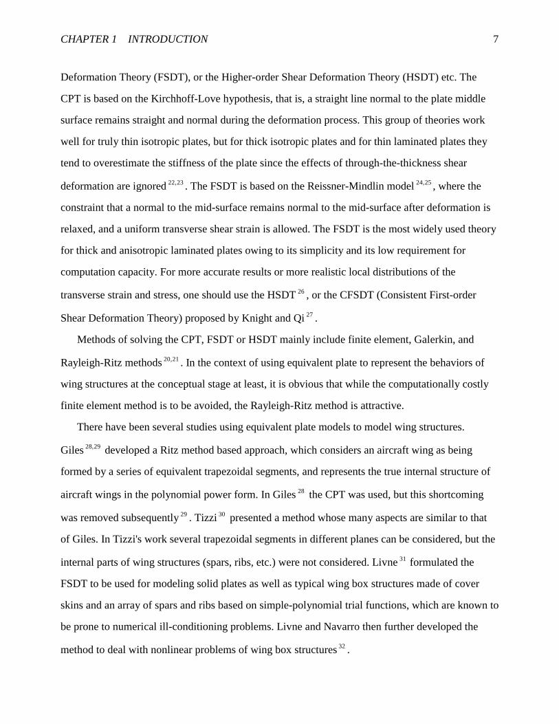
Deformation Theory (FSDT), or the Higher-order Shear Deformation Theory (HSDT) etc. The
CPT is based on the Kirchhoff-Love hypothesis, that is, a straight line normal to the plate middle
surface remains straight and normal during the deformation process. This group of theories work
well for truly thin isotropic plates, but for thick isotropic plates and for thin laminated plates they
tend to overestimate the stiffness of the plate since the effects of through-the-thickness shear
deformation are ignored23,22 . The FSDT is based on the Reissner-Mindlin model25,24 , where the
constraint that a normal to the mid-surface remains normal to the mid-surface after deformation is
relaxed, and a uniform transverse shear strain is allowed. The FSDT is the most widely used theory
for thick and anisotropic laminated plates owing to its simplicity and its low requirement for
computation capacity. For more accurate results or more realistic local distributions of the
transverse strain and stress, one should use the HSDT26 , or the CFSDT (Consistent First-order
Shear Deformation Theory) proposed by Knight and Qi27 .
Methods of solving the CPT, FSDT or HSDT mainly include finite element, Galerkin, and
Rayleigh-Ritz methods 21,20 . In the context of using equivalent plate to represent the behaviors of
wing structures at the conceptual stage at least, it is obvious that while the computationally costly
finite element method is to be avoided, the Rayleigh-Ritz method is attractive.
There have been several studies using equivalent plate models to model wing structures.
Giles 29,28 developed a Ritz method based approach, which considers an aircraft wing as being
formed by a series of equivalent trapezoidal segments, and represents the true internal structure of
aircraft wings in the polynomial power form. In Giles28 the CPT was used, but this shortcoming
was removed subsequently29 . Tizzi30 presented a method whose many aspects are similar to that
of Giles. In Tizzi's work several trapezoidal segments in different planes can be considered, but the
internal parts of wing structures (spars, ribs, etc.) were not considered. Livne31 formulated the
FSDT to be used for modeling solid plates as well as typical wing box structures made of cover
skins and an array of spars and ribs based on simple-polynomial trial functions, which are known to
be prone to numerical ill-conditioning problems. Livne and Navarro then further developed the
method to deal with nonlinear problems of wing box structures32 .

CHAPTER 1 INTRODUCTION 8
1.5 Sensitivity Techniques
Sensitivity techniques are frequently used in structural design practices for searching the
optimal solutions near a baseline design35~33 . The design parameters for wing structure include
sizing-type variables (skin thickness, spar or rib sectional area etc.), shape variables (the plan
surface dimensions and ratios), and topological variables (total spar or rib number, wing topology
arrangements etc.). Sensitivities to the shape variables are extremely important because of the
nonlinear dependence of stiffness and mass terms on the shape design variables as compared to the
linear dependence on the sizing-type design variables.
Kapania and coworkers have addressed the first order shape sensitivities of the modal response,
divergence and flutter speed, and divergence dynamic pressure of laminated, box-wing or general
trapezoidal built-up wing composed of skins, spars and ribs using various approaches of
determining the response sensitivities42~36 .
1.6 Scope of the Present Work
The aim of the present work is trying to develop efficient methods for the structural analysis of
built-up wings at the early design stage, such that with a fraction of the computational cost of a
detailed FEA, sufficiently accurate results for the global properties of the wing can be obtained. In
the present study, continuum models, neural networks and some other efficient simulation tools are
going to be used to make the objective possible.
As a preparation for application in later chapters, basic concepts and formulations about two
most commonly used neural networks, the Feed-Forward NN and Radial Basis Function NN, are
described in Chapter 2. Details of how to use some basic functions in the MATLAB NN Toolbox
for training and testing networks are provided, together with two ways of application of neural
networks: the direct approach and the indirect approach.

CHAPTER 1 INTRODUCTION 9
Chapter 3 is composed of an introduction of the continuum models used by several authors,
and an example of treating a lattice structure with repeating cells by continuum modeling applying
neural networks, compared with results obtained by other authors.
The present study is an extension of the previous works of Kapania and Singhvi44,43 , Kapania
and Lovejoy 46,45,21,20 , and Cortial47 , who all used the Rayleigh-Ritz method with the Chebyshev
polynomials as the trial functions, and applied the Lagrange’s equations to obtain the stiffness and
mass matrices. In Kapania and Singhvi44,43 , the CPT was used to solve generally laminated
trapezoidal plates, while in Kapania and Lovejoy 46,45,21,20 , the FSDT was used. In all these studies,
only uniform plates were considered. In Cortial47 , efforts were made to use the method of Kapania
and Lovejoy 46,45,21,20 to calculate natural frequencies of box-wing structures, but an assumption of
constant wing thickness makes it difficult to apply the method to general wing structures.
In the present work, it is assumed that the wing plan form is quadrilateral, and the wing
structure is composed of skins, spars and ribs. The wing is represented as an equivalent plate
model, and the Reissner-Mindlin displacement field model is used. The Rayleigh-Ritz method is
applied to solve the plate problem, with the Legendre polynomials being used as the trial functions.
After the stiffness matrix and mass matrix are determined by applying the Lagrange’s equations,
static analysis can be readily performed and the natural frequencies and mode shapes of the wing
can be obtained by solving an eigenvalue problem. Formulations are such that there is no limitation
on the wing thickness distribution as was the case in Cortial47 . This basic part of work, a method to
solve the Mindlin plates, is contained in Chapter 4. Then the method, being called the Equivalent
Plate Analysis (EPA), is applied for solving built-up wing structures in Chapter 5. As examples of
verifying EPA, a wing-shaped plate, a wing-shaped plate with camber, a solid wing and a general
built-up wing are analyzed respectively, and the results are compared with those obtained from a
detailed FE analysis using MSC/NASTRAN.
The EPA as explained above can also be used as a basis for generating other efficient methods
in the design of wing structures, such that can be incorporated with optimization tools into the
process of searching for an optimal design. In the search for an optimal design, it is essential to

CHAPTER 1 INTRODUCTION10
assess the structural responses quickly at any design space point. For such purpose, the FEM or
even the above EPA, which establishes the stiffness and mass matrices by integrating contributions
spar by spar, rib by rib, are not efficient enough.
One approach is to use Neural Networks as a means of simulating the structural responses of
wings. This is the so called direct application of neural networks, as discussed in Chapter 2.
Another approach is to use the sensitivity techniques. Sensitivity techniques are frequently used in
structural design practices for searching the optimal solutions near a baseline design34,33 . In the
present work, the modal response of general trapezoidal wing structures is approximated using
shape sensitivities up to the 2nd order, and the use of second order sensitivities proved to be
yielding much better results than the case where only first order sensitivities are used. Also
different approaches of computing the derivatives are investigated. These two approaches of direct
simulation of modal wing responses are described in Chapter 6, along with an example showing
results giving by both approaches.
Finally, in Chapter 7, a method more efficient than the EPA with indirect application of neural
networks is developed. Instead of evaluating the matrices over all components of the wing
structure, evaluation is performed only over the skins, whose "equivalent" material constitutive
matrix and mass density distribution are changed accordingly to incorporate the effects of spars and
ribs. The new skin material properties are simulated using Neural Networks in terms of the wing
design variables. As it is shown, while the Neural-Network-aided EPA, which can be called
Equivalent Skin Analysis (ESA), gives almost equally good results, it uses only a fraction of the
CPU time spent in the ordinary EPA in generating the matrices.
Major parts of the present work are published. They include Chapter 4 and 5 in Ref. 48 and 49,
Chapter 6 in Ref. 50 and 51, and Chapter 7 in Ref. 52.

11
Chapter 2
Basics of Neural Networks
In this chapter a brief description is given to the most extensively used neural network in civil and
structural engineering, Multi-Layer Feed-Forward NN, and another kind of NN, Radial Basis
Function NN, which is very efficient in some cases. Some conceptual features of NN are listed.
Several functions of MATLAB NN Toolbox are introduced, which will be used as the major tools in
the present work. At the end of this chapter a brief discussion is made on approaches of application
of neural networks.
2.1 Two Important Types of NN
As simplified models of the biological brain, ANNs have lots of variations due to specific
requirements of their tasks by adopting different degree of network complexity, type of inter-
connection, choice of transfer function, and even differences in training method.
According to the types of network, there are Single Neuron network (1-input , 1-output, and no
hidden layer), Single-Layer NN or Percepton (no hidden layer), and Multi-Layer NN (1 or more
hidden layers). According to the types of inter-connection, there are Feed-Forward network (values
can only be sent from neurons of a layer to the next layer), Feed-Backward network (values can
only be sent in the different direction, i.e. from the present layer to the previous layer), and
Recurrent network (values can be sent in both directions).

CHAPTER 2 BASICS OF NEURAL NETWORKS 12
In the following a brief description is given to two kinds of extensively used neural networks
and some of the pertinent concepts.
2.1.1 Feed-Forward Multi-Layer Neural Network
An example of feed-forward multi-layer neural network is shown in Fig. 2.1, where the
numbers of input and output are 3 and 2 respectively, and there are two hidden layers with 5
neurons in the first hidden layer, and 3 neurons in the second hidden layer. The details of a neuron
is illustrated in Fig. 2.2. As shown in Fig. 2.2, in the j -th layer, the i -th neuron has inputs from
the )1( −j -th layer of value ),,1( 11
−− = j
jk nkx � , and has the following output
)( ji
ji rfx = (2.1)
where
ji
n
k
jk
jki
ji bxwr
j
−= ∑−
=
−−1
1
11 (2.2)
in which 1−jkiw is the weight between node k of the )1( −j -th layer and node i of the j -th layer,
and jib is the bias (also called threshold). The above relation can also be written as
∑−
=
−−=1
0
11jn
k
jk
jki
ji xwr (2.3)
where ji
j bx =−10 and 11 −=−j
oiw , or 110 −=−jx and j
ij
oi bw =−1 .

CHAPTER 2 BASICS OF NEURAL NETWORKS 13
inputlayer
hiddenlayers
outputlayer
Fig. 2.1 A feed-forward multi-layer neural network
Σ f ( ).xi
jr ij
w k ij - 1
-1
.
.
.
.
.
.
bij
x1j -1
x2j-1
k= n j-1
w 1 ij - 1
w 2 ij - 1
xkj -1
T rans ferfunc tio n
S ummingjunc tion
O utput
Inputs ignals
Synapticweights
T hresho ld
Fig. 2.2 Details of a neuron

CHAPTER 2 BASICS OF NEURAL NETWORKS 14
The transfer function (also called activation function or threshold function) is usually specified
as the following Sigmoid function
rerf −+
=1
1)( . (2.4)
Other choices of the transfer function can be the hyperbolic tangent function
r
r
e
erf −
−
+−=
1
1)( , (2.5)
the piece-wise linear function
≤≤≤−+
≥=
.5.0,0
;5.05.0,5.0
;5.0,1
)(
r
rr
r
rf (2.6)
and, sometimes, the 'pure' linear function
.)( rrf = (2.7)
These transfer functions are displayed in Fig. 2.3.
r
f(r)
-5 0 5-1
-0.75
-0.5
-0.25
0
0.25
0.5
0.75
1
Linear
Hyperbolic tangent
Sigmoid
Piecewise-linear
Fig. 2.3 Transfer functions

CHAPTER 2 BASICS OF NEURAL NETWORKS 15
n1 n2 n3number ofneurons:
inputlayer
hiddenlayer
outputlayer
Fig. 2.4 Radial basis function neural network
2.1.2 Radial Basis Function Neural Network
Radial Basis Function (RBF) NN usually have one input layer, one hidden layer and one output
layer, as shown in Fig. 2.4.
For the RBF network in Fig. 2.4, we have the relations between the input 1ix (here 1,,1 ni �= )
and the output 2kx (here 3,,1 nk �= ) as follows:
2
1
2,
22
k
n
jjjkk brwx += ∑
=
(2.8)
∑=
=1
1
1,
11 ),,(n
ijijij bwxGr (2.9)
where 2w , 2b are the weights and bias respectively, and the Gaussian function is used as the
transfer function:
)}{}{exp(),,( 21121,
1,
11jijijiji wxbbwxG −−= (2.10)
where 1w is the center vector of the input data, and 1b is the variance vector.

CHAPTER 2 BASICS OF NEURAL NETWORKS 16
2.2 Features of ANN
Some important features of NN are briefed as follows.
• Many NN methods are universal approximators, in the sense that, given a dimension (number
of hidden layers and neurons of each layer) large enough, any continuous mapping can be
realized. Fortunately, the two NNs we are most interested in, the multi-layer feed-forward NN
and the radial basis function NN, are examples of such universal approximators54,53 .
• Steps of utilizing NN: specification of the structure (topology)→ training (learning)
→ simulation (recalling).
(1) Choosing structural and initial parameters (number of layers, number of neurons of each
layer, and initial values of weights and thresholds, and the kind of transfer function) is usually
from experiences of the user and sometimes can be provided by the algorithms. (2) The training
process uses given input and output data sets to determine the optimal combination of weights
and thresholds. It is the major and the most time-consuming part of NN modeling, and there are
lots of methods regarding different types of NN. (3) Simulation means using the trained NN to
predict output according to new inputs (This corresponds to the 'recall' function of the brain).
• The input and output relationship of NN is highly nonlinear. This is mainly introduced by the
nonlinear transfer function. Some networks, e.g. the so-called "abductive" networks, use double
even triple powers besides linear terms in their layer to layer input-output relations55 .
• A NN is parallel in nature, so it can make computation fast. Neural networks are ideal for
implementation in parallel computers. Though NN is usually simulated in ordinary computers
in a sequential manner.
• A NN provides general mechanisms for building models from data, or give a general means to
set up input-output mapping. The input and output can be continuous (numerical), or not
continuous (binary, or of patterns).
• Training a NN is an optimization process based on minimizing some kind of difference
between the observed data and the predicted while varying the weights and thresholds. For

CHAPTER 2 BASICS OF NEURAL NETWORKS 17
numerical modeling, which is of our major concern for the present study, there is a great
similarity between NN training and some kind of least-square fitting or interpolation.
• Simulation using NN gives better results in interpolation than in extrapolation, the same as any
other data fitting or mapping methods.
• Where and when to use NN depend on the situation, and NN is not a panacea. The following
comment on NN application on structural engineering seemingly can be generalized in other
areas:
"The real usefulness of neural networks in structural engineering is not in reproducing existing
algorithmic approaches for predicting structural responses, as a computationally efficient
alternative, but in providing concise relationships that capture previous design and analysis
experiences that are useful for making design decisions"7 .
Despite the above features and wide application in a lot of areas, there seems to be no evidence
for neural networks to claim superiority over some other mapping tools. For instance, in a recent
paper of Nikolaidis, Long, and Ling 73, it is claimed that the response surface polynomials with
stepwise regression and the neural network models appear to be almost equally accurate, but it took
considerably less time to develop the polynomials than the neural networks.
2.3 Algorithms in the MATLAB Neural Network Toolbox
When using MATLAB NN Toolbox, one should first choose the number of input and output
variables. This is accomplished by specifying the two matrices p and t , where p is a nm×
matrix; m is the number of input variables, and n the number of sets of training data; and t is a
nl × matrix; l is the number of output variables. The number of network layers, and numbers of
neurons of each layer are other factors that need to be specified.
MATLAB gives algorithms for specifying initial values of weights and thresholds in order that
training can be started. For feed-forward NN, function initff is given for this purpose. The
following is an example of using the algorithm

CHAPTER 2 BASICS OF NEURAL NETWORKS 18
[w1,b1,w2,b2,w3,b3]=initff(p,n1,'logsig',n2,'logsig',t,'logsig');
where w1, w2, and w3 are initial values for the weight matrices of the 1st (hidden), 2nd (hidden)
and 3rd (output) layer respectively, b1, b2, and b3 are the bias (threshold) vectors, n1 and n2 the
number of neurons in the 1st and 2nd hidden layer respectively, and 'logsig' means that the Sigmoid
transfer function is used.
The present version of MATLAB NN Toolbox can support only 2 hidden layers, but the number
of neurons is only limited by the available memory of the computer system being used. For the
transfer function, one can also use other choices, such as 'tansig' (hyperbolic tangent sigmoid),
'radbas' (radial basis) and 'purelin' (linear) etc.
Experiences of using initff indicated that it seems to be a random process since it is found that
the result of the execution of this algorithm each time is different. And other conditions kept the
same, two executions of this function usually give quite different converging histories of training
by the training algorithm8 .
Shown in the following is the MATLAB algorithm for training feed-forward network with back-
propagation:
[w1,b1,w2,b2,w3,b3,ep,tr]=trainbp(w1,b1,'logsig',w2,b2,'logsig',w3,b3,'logsig',p,t,tp);
where most of the parameters which the user should take care of have been mentioned in the above
paragraphs. The only parameter that the user sometimes need to specify is the 41× vector tp,
where the first element indicates the number of iterations between updating displays, the second the
maximum number of iterations of training after which the algorithm would automatically terminate
the training process, the third the converging criterion (sum-squared error goal), and the last the
learning rate. The default value of tp is [25, 100, 0.02, 0.01].
Other algorithms for training include trainbpa (training feed-forward NN with back-
propagation and adaptive learning), solverb (designing and training radial basis network), and
trainlm (training feed-forward NN with Levenberg-Marquardt algorithm) etc.
trainbpa and trainlm have very similar formats for using as that of trainbp. The radial basis
network designing and training algorithm has the following format

CHAPTER 2 BASICS OF NEURAL NETWORKS 19
[w1,b1,w2,b2,nr,err]=solverb(p,t,tp);
where the algorithm chooses centers for the Gaussians and increases the neuron number of the
hidden layer automatically if the training cannot converge to the given error goal. So it is also a
designing algorithm.
After the NN is trained, one can predict output from input by using simulation algorithms in
terms of the obtained parameters w1, b1, w2, b2, etc. For feed-forward network one use
y=simuff(x,w1,b1,'logsig',w2,b2,'logsig',w3,b3,'logsig');
where x is the input matrix, and y the predicted output matrix. Similarly, after a radial basis
network has been trained one uses
y=simurb(x,w1,b1,w2,b2);
to predict the output.
Once a NN is trained, we can use the formulations in 2.1 or 2.2 together with the obtained
parameters (weights etc.) to setup the network to do prediction anywhere and not necessarily within
the MATLAB environment.
2.4 Ways of Application of Neural Networks
For the efficient simulation of the structural performances of complex wings, there can be two
directions to apply NN as specified in the following:
2.4.1 Direct Application
In this case, the input layer includes all the design variables of interest (for instance, the four
shape parameters of the wing plan form: the sweep angle, the aspect ratio, the taper ratio, and the
plan area). The output layer gives the desired structural responses, such as natural frequencies etc.
The EPA is being used as the training data generator, though if necessary, results obtained using
the FEA can also be used as the training data. Preparation of training data is very important, and the
training algorithm used also greatly impacts the process of training8 . Caution must be taken in
specifying the network parameters and training criterion, such that the results of the trained

CHAPTER 2 BASICS OF NEURAL NETWORKS 20
network would not oscillate around the training data. Once the networks are trained, structural
responses at any design point can be recalled in a fraction of a second and this is really favorable in
a design situation51.
2.4.2 Indirect Application
Here it is desired to find a way of incorporating NN into the application of the equivalent plate
analysis (EPA) of complex wing structures, other than just making use of results generated by EPA
as the training data base. Note that in the EPA of a complex wing, the computational effort is
mainly spent on integrals for generating the contribution from the inner-structural components of
the wing, i.e. the spars and the ribs, in the stiffness and mass matrices. If an anisotropic material
can be found to replace the inner components, in terms of an equivalent skin, such that the new
composite wing has very close global properties as the original one, then the EPA can be
performed more efficiently. Solution of the adequate material properties of the anisotropic material
is the major obstacle here. The role of NN will be relating the material properties to all kinds of
wing design parameters, and it can be trained when there exists enough data base for training. This
way of applying NN has been claimed to be the best use of the Neural Networks in structural
engineering7 . This is the path that is to be followed in Chapter 7.

21
Chapter 3
Continuum Model Approaches
3.1 Methods of Obtaining Continuum Models
A lot of methods have been used to develop continuum models to represent complex structures.
Many of these methods involve the determination of the appropriate relationships between the
geometric and material properties of the original structure and its continuum models. An important
observation is that the continuum model is not unique, and determining the continuum model for a
given complex structure is inherently ill-posed therefore diverse approaches can be used. This can
be clearly shown in the following example of determining continuum models for a lattice structure.
The single-bay double-laced lattice structure shown in Fig. 3.1 has been studied in Ref. 10, 12,
and 14 with different approaches to the continuum modeling. This lattice structure with repeating
cells can be modeled by a continuum beam if the beam's properties is properly provided.
Noor et al's method include the following steps10: (1)introducing assumptions regarding the
variation of the displacements and temperature in the plane of the cross section for the beamlike
lattice, (2)expressing the strains in the individual elements in terms of the strain components in the
assumed coordinate directions, (3)expanding each of the strain components in a Taylor series, and
(4)summing up the thermoelastic strain energy of the repeating elements which then gives the
thermoelastic and dynamic coefficients for the beam model in terms of material properties and
geometry of the original lattice structure.

CHAPTER 3 CONTINUUM MODEL APPROACHES 22
Lg
Lc
longitudinal bar
diagonal bar
batten
In Sun et al12, the properties of the continuum model is obtained respectively by relating the
deformation of the repeating cell to different load settings under specified boundary conditions. For
example, the shear rigidity GA is obtained by performing a numerical shear test in which a unit
shear force is applied at one end of the repeating cell and the corresponding shear deformation is
calculated by using a finite element program. The mass and rotatory inertia are calculated with a
averaging procedure.
Lee put forward a method that he thought to be more straightforward14. He used an extended
Timoshenko beam to model the equivalent continuum beam. By expressing the total strain and
kinetic energy of the repeating cell in terms of the displacement vector at both ends of the
continuum model, and equating them to those obtained through the extended Timoshenko beam
Length of longitudinal bars: cL Length of battens: gL
Length of diagonal bars: 21
)( 22gcd LLL += Areas: ,cA ,gA dA
Fig. 3.1 Geometry of repeating cells of a single-bay double laced lattice structure

CHAPTER 3 CONTINUUM MODEL APPROACHES 23
theory, he got a group of relations. The number of these relations, 2N(1+2N), where N is the degree
of freedom of the continuum model, is usually larger than that of the equivalent continuum beam
properties to be determined. Lee then introduced a procedure in which the stiffness and mass
matrices for both the lattice cell and the continuum model are reduced and so is the number of
relations. Yet how to reduce the number of relations to be equal to the number of unknowns seems
to depend on luck.
All the above three methods give close results for the continuum model properties, and the
continuum models also generate promising global results for the lattice structure.
3.2 An Example of NN Modeling of Continuum Models
Emphasizing the application of NN, we choose an approach similar to that in Ref. 12, that is, to
derive the properties of the beam by investigating the force-deformation relationships of the
repeating cell in certain boundary conditions. The approach is illustrated in Fig. 3.2, where the
beam's axial rigidity EA, bending rigidity EI, and shearing rigidity GA are calculated respectively
by using the results of finite element analysis of the repeating cell in different load conditions.
Concerning the finite element analysis of 3-D lattice structures one can consult Ref. 56.
There are five parameters of the repeating cell for the lattice structure in Fig. 3.1 that can be
varied, the longitudinal bar length cL , the batten length gL , and the longitudinal, batten and
diagonal bar area, cA , gA and dA . Generally, a function with more variables will be more complex
and it will be more difficult for a neural network to simulate its performance. A NN with more
input variables needs much more training data since in the training data each variable should vary
separately. As can be shown in the following, this kind of "coarse" training data pose an obstacle to
most of the training algorithms.
Three scenarios were investigated, with the number of input variables set to be 2, 3 and 4
respectively.

CHAPTER 3 CONTINUUM MODEL APPROACHES 24
1
2
3
4
5
6
x, u
y, v
1/31/3
1/3
z, w
1
2
3
4
5
6
x, u
y, v
1/31/3
1/3
z, w
1
2
3
4
5
6
x, u
y, v
1/21/2
1
z, w
3.2.1 Neural Network with 2 Input Variables
The input variables are cL and cA . The number of training data sets is 400=20× 20. The
number of testing data, most of which are located at centers among the training data mesh, is also
400=20× 20. Part of the results, as the training data, about GA, is shown in Fig. 3.3.Positions of the
training as well as the testing data points are shown in Fig. 3.4. Simulations on the testing data and
the relative errors of a 2-10-1 FF NN (feed-forward neural network with 2 inputs, one hidden layer
of 10 neurons, and 1 output) trained with Levenberg-Marquardt algorithm (trainlm) are shown in
Axial rigidity EA:
641
521
441 vvv
L
v
LEA cc
++≅
∆=
Bending rigidity EI:
45
243
23
231
vv
LLLLEI
LEILM
cgcg
c
g
−≅=⇒
⋅=×=
φ
φShear rigidity GA:
641
521
441
641
521
441
11
www
L
GA
c
++=
++≅=
θθθθ
Fig. 3.2 Evaluating continuum model properties for a repeating cell

CHAPTER 3 CONTINUUM MODEL APPROACHES 25
Figs. 3.5 and 3.6. Results of a radial-basis-function (RBF) NN doing the same job are shown in
Figs. 3.7 and 3.8. In both cases the training error criteria were set to be 3104.0 −× .
From Figs 3.5 and 3.7 we can see that both the FF NN and RBF NN give a very good
simulation of the relation ),( cc LAfGA= , except at points outside the training data range of
variable cL ( cf. Fig. 3.4). At the "inside" points, or positions where interpolations are made, the
abstract values of the relative errors are well below the 1%. On the other hand, at points outside the
training data range of variable cL , the relative errors can be as high as 3~5%. This provides another
proof to the fact mentioned before, that interpolation using NN will give results more accurate than
extrapolation.

CHAPTER 3 CONTINUUM MODEL APPROACHES 26
1.5
2
2.5
3
GA
0
1
2Ac(m
2 )
0
2
4
6
8
10
12
Lc(m)
X Y
Z
GA Training Data
x10-4
x106
Lc(m)
Ac(
m2 )
0 2 4 6 8 10 120
0.2
0.4
0.6
0.8
1
1.2
1.4
1.6
1.8
2
2.2
2.4Testing pointsTraining points
Training & Testing Points
x10-4
Fig. 3.3 Training data for )( , cc LAfGA=
Fig. 3.4 Distributions of training and testing points

CHAPTER 3 CONTINUUM MODEL APPROACHES 27
2
3
GA
(FF
)
0
0.5
1
1.5
2Ac(m
2 )
0
2
4
6
8
10
12
Lc(m)
X Y
Z
FF Simulation on Testing Data
x10-4
x106
-4
-2
0
2
{GA
-GA
(FF
)}/G
A
0.5
1
1.5
2
Ac(m2 )
2
4
6
8
10
Lc(m)
0.49
-0.070.49
-2.85
-1.18-0.62 -0.07-0.07
-0.07
-0.07-0.07
X Y
Z
FF Simulation Errors
x10-4
x10-2
Fig. 3.5 Feed-forward NN simulation for )( , cc LAfGA=
Fig. 3.6 Feed-forward NN simulation errors

CHAPTER 3 CONTINUUM MODEL APPROACHES 28
2
3
GA
(RB
F)
0
1
2Ac(m
2 )
0
2
4
6
8
10
12
Lc(m)
X Y
Z
RBF Simulation on Testing Data
x10-4
x106
0
2
4
{GA
-GA
(RB
F)}
/GA
0
1
2Ac(m
2 )
0
2
4
6
8
10
12
Lc(m)
0.90
0.90
-0.15
1.96
0.380.901.96
-0.15
1.43
1.431.962.48
0.901.43
-0.15
-0.15
-0.15
-0.1
5
X Y
Z
RBF Simulation Errors
x10-2
x10-4
Fig. 3.7 Radial-basis function NN simulation for )( , cc LAfGA=
Fig. 3.8 Radial-basis function NN simulation errors

CHAPTER 3 CONTINUUM MODEL APPROACHES 29
3.2.2 Neural Network with 3 Input Variables
The input variables were chosen as cL , cA and dA . The number of training data sets is
343=7× 7× 7. For this case, the effectiveness of different training algorithms can be seen clearly in
Figs. 3.9~3.11. When ordinary back-propagation training algorithm, i.e. trainbp is used, it is very
hard to train the NN to the error level of 110− , as shown in Fig. 3.9. When the adaptive learning
technique is included, an improvement can be made, but it is still hard to reach the 210− error level,
as can be seen in Fig. 3.10. Now if the algorithm with Levenberg-Marquardt (trainlm) is used, it is
quite easy to push the training error level to the order of 510− , as shown in Fig. 3.11.
The improvement by trainlm is really amazing. All the training algorithms carry out an
optimization process. While trainbp uses steepest-descent method with constant step size, trainbpa
accelerates the process by adjusting the step size. On the other hand, trainlm adopts a kind of
modified Newton's Methods, which adjusts both the searching direction and the step size.
Concerning the optimization methods one can consult Ref. 57.
Samples of the NN simulation results are given in Table 3.1, where the desired values and
values obtained by Noor et al10 and Lee14 are also presented.
3.2.3 Neural Network with 4 Input Variables
The input variables were chosen as cL , cA , gA and dA .The number of training data sets is
625=5× 5× 5× 5. For this case only trainlm could train a FF NN that could give reasonable results.
Samples of the NN simulation results are given in Table 3.2.

CHAPTER 3 CONTINUUM MODEL APPROACHES 30
Epoch
Sum
-Squ
ared
Err
or
0 5000 10000 15000 20000
10-1
100
101
Epoch
Sum
-Squ
ared
Erro
r
0 5000 10000 15000 20000
10-1
100
101
102
Fig. 3.9 Training history of a 3-10-1 feed-forward NN by trainbp
Fig. 3.10 Training history of a 3-10-1 feed-forward NN by trainbpa

CHAPTER 3 CONTINUUM MODEL APPROACHES 31
Epoch
Sum
-Squ
ared
Err
or
0 50 100 150 200 250
10-5
10-4
10-3
10-2
10-1
100
101
Table 3.1 Comparison of Continuum Model Properties for a Lattice Repeating CellFeatures of the cell: 25210 106,0.5,/1017.7 mAmLmNE gg
−×==×=
Variables specified: 2525 104,108,5.7 mAmAmL dcc−− ×=×==
Present(FEA)
present (FFsimulated, trained
by trainbpa, 3variables)
present(RBF
simulated,3vaiables)
present (FFsimulated, trained
by trainlm, 3variables)
U. Lee Noor etal
EA( )107 N 2.659 2.60 2.66 2.656 2.71 2.53
GA( )106 N 2.183 2.24 2.17 2.186 2.2 2.2
EI( )10 27 mN ⋅ 8.147 8.08 8.17 8.148 8.20 8.01
Table 3.2 Comparison of Continuum Model Properties for a Lattice Repeating CellFeatures of the cell: mLmNE g 0.5,/1017.7 210 =×=
Variables specified: 252525 106,104,108,5.7 mAmAmAmL gdcc−−− ×=×=×==
Present(FEA)
present (FF simulated, trainedby trainlm, 4 variables)
U. Lee Noor et al
EA( )107 N 2.659 2.682 2.71 2.53
GA( )106 N 2.183 2.134 2.2 2.2
EI( )10 27 mN ⋅ 8.147 8.181 8.20 8.01
Fig. 3.11 Training history of a 3-10-1 feed-forward NN by trainlm

32
Chapter 4
An Approach for the Solution of Mindlin
Plates
In this chapter a FSDT (the Reissner-Mindlin theory) method, using the Ritz method with the
Legendre or the Chebyshev polynomials being employed as the trial functions, is derived to solve
plate problems. Formulations are such that there is no limitation on the plate thickness variation
and therefore can be used to deal with real-life wings in the next chapter.
4.1 Assumptions and Formulations
For the solution of a plate under static or dynamic deformation, the Reissner-Mindlin method, a
First-order Shear Deformation Theory (FSDT), is based on two assumptions for the displacement
field: (1) A normal line to the non-deformed middle surface remains to be a straight line; (2) The
transverse normal stress can be neglected in the constitutive relations.
According to these assumptions, and assuming linearity, the displacement field of the plate is
given as:
=+=+=
),,(),,,(
),,(),,(),,,(
),,(),,(),,,(
0
0
0
tyxwtzyxw
tyxztyxvtzyxv
tyxztyxutzyxu
y
x
φφ
(4.1)

CHAPTER 4 AN APPROACH FOR MINDLIN PLATES 33
where as shown in Fig. 4.1, wvu ,, are displacements in the zyx ,, direction respectively, subscript
0 refers to quantities associated with the plane 0=z , xφ and yφ are the rotations about the y and
x− direction respectively. It is assumed here that the middle surface of the plate is without or with
a very small curvature, therefore 0=z can be considered to be the middle surface.
From Eq. (4.1) we can get the strains:
∂∂+=
∂∂+
∂∂==
∂∂+=
∂∂+
∂∂==
∂∂
+∂∂+
∂∂+
∂∂=
∂∂+
∂∂==
=∂∂=
∂∂
+∂∂=
∂∂=
∂∂+
∂∂=
∂∂=
x
w
z
u
x
wy
w
y
w
z
vxy
zx
v
y
u
x
v
y
uz
wy
zy
v
y
vx
zx
u
x
u
xzxzx
yyzyz
yxxyxy
z
yy
xx
0
0
00
0
0
2
2
)(2
0
φεγ
φεγ
φφεγ
ε
φε
φε
(4.2)
For the convenience of calculation, a transformation from ),( yx to ),( ηξ is performed, with
the plate configuration in the ),( yx plane being transformed to a square in the ),( ηξ plane, as
shown in Fig. 4.1. The plate configuration in the ),( yx plane can be any quadrilaterals, of which a
special case, the skewed trapezoidal, is frequently used in aircraft wing configurations.
x, u
z, w y, v
1
2
4
3
z
ξ
η
(1,-1) (1,1)
(-1,-1) (-1,1)
Fig. 4.1 The coordinate system and its transformation

CHAPTER 4 AN APPROACH FOR MINDLIN PLATES 34
The transformation can be formulated as
=
=
∑
∑
=
=4
1
4
1
),(
),(
iii
iii
yNy
xNx
ηξ
ηξ (4.3)
where
+−=++=−+=−−=
)1)(1(),(
)1)(1(),(
)1)(1(),(
)1)(1(),(
41
4
41
3
41
2
41
1
ηξηξηξηξηξηξηξηξ
N
N
N
N
(4.4)
The Jacobian matrix for this transformation is
∂∂
∂∂
∂∂
∂∂
=
ηξ
ηξyy
xx
J ][ (4.5)
where from Eqs. (4.3) and (4.4) it is ready to obtain
−−+−+=∂∂
−−+−+=∂∂
−−+−+=∂∂
−−+−+=∂∂
)])(1())(1[(
)])(1())(1[(
)])(1())(1[(
)])(1())(1[(
142341
124341
142341
124341
yyyyy
yyyyy
xxxxx
xxxxx
ξξη
ηηξ
ξξη
ηηξ
. (4.6)
The inverse of the Jacobian matrix:
=
−
−=
∂∂
∂∂−
∂∂−
∂∂
=−
2221
1211
1121
12221 1][
JJ
JJ
JJ
JJ
JJ
xy
xy
Jξξ
ηη
(4.7)
where J is the determinant of the Jacobian:

CHAPTER 4 AN APPROACH FOR MINDLIN PLATES 35
∂∂
∂∂−
∂∂
∂∂=
ξηηξyxyx
J . (4.8)
We express the terms on the plane 0=z in Eq. (4.1), i.e. 0u , 0v , 0w , xφ and yφ , in the
following forms
==
==
==
==
==
∑∑
∑∑
∑∑
∑∑
∑∑
= =
= =
= =
= =
= =
R
r
S
ssrrsY
TRSy
P
p
Q
qqppqX
TPQx
M
m
N
nnmmnW
TMN
K
k
L
llkklV
TKL
I
i
J
jjiijU
TIJ
BBtYqB
BBtXqB
BBtWqBw
BBtVqBv
BBtUqBu
1 1
1 1
1 10
1 10
1 10
)()()(}{}{
)()()(}{}{
)()()(}{}{
)()()(}{}{
)()()(}{}{
ηξφ
ηξφ
ηξ
ηξ
ηξ
(4.9)
or
}{}{
}{
}{
}{
}{
}{
}}{,}{,}{,}{,}{{0
0
0
qB
q
q
q
q
q
BBBBBw
v
u
T
Y
X
W
V
U
TRS
TPQ
TMN
TKL
TIJ
y
x
=
=
φφ
(4.10)
where RQPNMLKJI ,,,,,,,, and S are integers,
====
==
TRSY
TPQX
TMNW
TKLV
TIJIJJU
TTY
TX
TW
TV
TU
YYqXXq
WWqVVq
UUUUUUUq
qqqqqq
},,{}{,},,{}{
},,{}{,},,{}{
},,,,,,,,,,{}{
}}{,}{,}{,}{,}{{}{
1111
1111
122111211
��
��
���� (4.11)
is called the generalized displacement vector, and
=
=
=
RSPQMNKLIJ
BBBBB
BBBBBBT
TTRS
TPQ
TMN
TKL
TIJ
,,,,
)}()(,),()({}{
}}{,}{,}{,}{,}{{}{
11
µνηξηξ νµµν � (4.12)
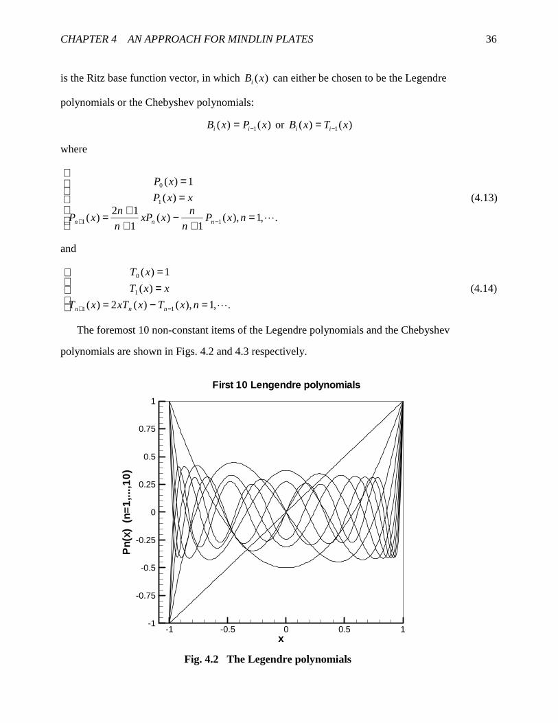
CHAPTER 4 AN APPROACH FOR MINDLIN PLATES 36
is the Ritz base function vector, in which )(xBi can either be chosen to be the Legendre
polynomials or the Chebyshev polynomials:
)()( 1 xPxB ii −= or )()( 1 xTxB ii −=
where
=+
−++=
==
−+ .,1),(1
)(1
12)(
)(
1)(
11
1
0
�nxPn
nxxP
n
nxP
xxP
xP
nnn
(4.13)
and
=−===
−+ .,1),()(2)(
)(
1)(
11
1
0
�nxTxxTxT
xxT
xT
nnn
(4.14)
The foremost 10 non-constant items of the Legendre polynomials and the Chebyshev
polynomials are shown in Figs. 4.2 and 4.3 respectively.
x
Pn(
x)(n
=1
,...,1
0)
-1 -0.5 0 0.5 1-1
-0.75
-0.5
-0.25
0
0.25
0.5
0.75
1
First 10 Lengendre polynomials
Fig. 4.2 The Legendre polynomials

CHAPTER 4 AN APPROACH FOR MINDLIN PLATES 37
x
Tn(
x)(n
=1
,...,1
0)
-1 -0.5 0 0.5 1-1
-0.75
-0.5
-0.25
0
0.25
0.5
0.75
1
First 10 Cheb yshev pol ynomials
4.2 Strain Energy and Stiffness Matrix
The strain energy of a plate or a plate-like structure (for instance, a wing) is
∫∫∫=V
T dVU }{}{21 εσ (4.15)
Introducing the stress-strain relations by the generalized Hooke’s law, we have for Eq. (4.15)
∫∫∫=V
T dVDU }]{[}{21 εε (4.16)
Note that }]{[}{ εσ D= and ][][ DD T = is assumed, and the integration domain V in Eqs. (4.15)
and (4.16) includes all and only the spaces the components of the wing occupy.
Using Eqs. (4.5) and (4.7), we can write
Fig. 4.3 The Chebyshev polynomials

CHAPTER 4 AN APPROACH FOR MINDLIN PLATES 38
∂∂∂∂
=
∂∂∂∂
∂∂
∂∂
∂∂
∂∂
=
∂∂∂∂
y
fx
f
J
y
fx
f
yx
yx
f
f
T][
ηη
ξξ
η
ξ
∂∂∂∂
=
∂∂∂∂
=
∂∂∂∂
=
∂∂∂∂
∴ −−
η
ξ
η
ξ
η
ξf
f
JJ
JJf
f
Jf
f
J
y
fx
f
TT
2212
211111 )]([)]([ (4.17)
From Eqs. (4.2) and (4.17), we have
=
=
∂∂
∂∂
∂∂
∂∂
∂∂
∂∂
∂∂
∂∂
∂∂
∂∂
y
x
w
w
v
v
u
u
zx
yz
xy
y
x
y
y
x
x
JJ
JJ
JzJzJzJzJJJJ
JzJzJJ
JzJzJJ
φφ
εεεεε
ε
ηφ
ξφ
ηφ
ξφ
η
ξ
η
ξ
η
ξ
0
0
0
0
0
0
0100000000
1000000000
0000
00000000
00000000
}{
2111
2212
2111221221112212
22122212
21112111
= }]{[ εT (4.18)
From Eq. (4.9), we can write

CHAPTER 4 AN APPROACH FOR MINDLIN PLATES 39
}]{[
)()()(
)()()(
)()()(
)()()(
)()()(
)()()(
)()()(
)()()(
)()()(
)()()(
)()()(
)()()(
}{
1 1
1 1
1 1
1 1
1 1
1 1
1 1
1 1
1 1
1 1
1 1
1 1
0
0
0
0
0
0
qC
BBtU
BBtU
BBtU
BBtU
BBtU
BBtU
BBtU
BBtU
BBtU
BBtU
BBtU
BBtU
R
r
S
ssrrs
P
p
Q
qqppq
R
r
S
ssrrs
R
r
S
ssrrs
P
p
Q
qqppq
P
p
Q
qqppq
M
m
N
nnmmn
M
m
N
nnmmn
K
k
L
llkkl
K
k
L
llkkl
I
i
J
jjiij
I
i
J
jjiij
y
x
w
w
v
v
u
u
y
y
x
x=
′
′
′
′
′
′
′
′
′
′
=
=
∑∑
∑∑
∑∑
∑∑
∑∑
∑∑
∑∑
∑∑
∑∑
∑∑
∑∑
∑∑
= =
= =
= =
= =
= =
= =
= =
= =
= =
= =
= =
= =
∂∂
∂∂
∂∂
∂∂
∂∂
∂∂
∂∂
∂∂
∂∂
∂∂
ηξ
ηξ
ηξ
ηξ
ηξ
ηξ
ηξ
ηξ
ηξ
ηξ
ηξ
ηξ
φφ
ε
ηφ
ξφ
ηφ
ξφ
η
ξ
η
ξ
η
ξ
(4.19)
where
=
TRS
TPQ
RS
PQ
MN
KL
IJ
B
B
B
B
B
B
B
C
}{0000
0}{000
][0000
0][000
00][00
000][0
0000][
][
,
,
,
,
,
ξη
ξη
ξη
ξη
ξη
(4.20)
′′′
′′′=
)()()()()()(
)()()()()()(][
2111
2111
, ηξηξηξηξηξηξ
νµ
νµξηµν BBBBBB
BBBBBBB
�
�
TBBBBBBB })()()()()()({}{ 2111 ηξηξηξ νµµν �=
.,,,, RSPQMNKLIJ=µν
and }{q is the general displacement vector shown in Eq. (4.10).

CHAPTER 4 AN APPROACH FOR MINDLIN PLATES 40
Substitute Eqs. (4.18), (4.19) into Eq. (4.16), and we have
∫∫∫=V
TTT dVqCTDTCqU }]{][][[][][}{21 (4.21)
If we write
}]{[}{21 qKqU T= (4.22)
Then comparison of Eqs. (21) and (22) gives
∫∫∫=V
TT dVCTDTCK ]][][[][][][ (4.23)
This is the stiffness matrix of the plate in terms of }{q . Details for the constitutive matrix ][D
for different parts of the wing structure can be found in Appendix A.
4.3 Kinetic Energy and Mass Matrix
The kinetic energy of a plate or a plate-like structure (wing) is
∫∫∫ ∫∫∫==V V
T dVvvdVvT }{}{21
2
21 ρρ (4.24)
where the velocity vector
}]{][[
00100
0010
0001
}{ 0
0
0
0
0
0
•
∂∂
∂∂
∂∂
∂∂
∂∂
=
=
∂∂
∂∂
+∂∂
∂∂+
∂∂
=
∂∂= qHZz
z
t
wt
zt
vt
zt
u
t
dv
t
t
tw
tv
tu
y
x
y
x
φ
φ
φ
φ
(4.25)
where
=
00100
0010
0001
][ z
z
Z
=w
v
u
d}{ is the displacement vector, and

CHAPTER 4 AN APPROACH FOR MINDLIN PLATES 41
=
TRS
TPQ
TMN
TKL
TIJ
B
B
B
B
B
H
}{0000
0}{000
00}{00
000}{0
0000}{
][ (4.26)
and }{•q is the time-derivative of }{q .
Then we have
∫∫∫••
=V
TT dVqHZZHqT }]{][[][}{21 ρ (4.27)
where
==
2
2
000
000
00100
0010
0001
][][][
zz
zz
z
z
ZZZZ T (4.28)
Compare
}]{[}{21
••= qMqT T (4.29)
with Eq. (4.27) we have
∫∫∫=V
T dVHZZHM ]][[][][ ρ (4.30)
which is the mass matrix of the plate in terms of the general velocity vector, }{•q
It should be pointed out that the present formulation can deal with quadrilaterals of any shape
(see Fig.4.1), which include a skewed trapezoid, the usual shape for a wing plan form. Also, the
formulation can be extended to more complicated cases. When the wing plan form is composed of
several quadrilaterals or trapezoids, one can obtain the whole stiffness and mass matrices by
assembling the corresponding matrices of the component elements, as has been done in Tizzi30 . A
brief description of how to do in this kind of scenario can be found in Appendix B.

42
Chapter 5
Equivalent Plate Analysis of Built-Up Wing
Structures
Now we want to solve a wing problem by assuming that the wing behaves like a plate. This
assumption is very reasonable as long as the wing has a small thickness-chord ratio. The
formulations for a general quadrilateral plate derived in Chapter 4 will be used to deal trapezoidal
built-up wing structures in this chapter. This is accomplished by evaluating Eqs. (4.20) and (4.27)
for all the wing components. How to deal with the boundary conditions and the convergence
problem are discussed briefly. Once the total stiffness and mass matrices are determined, various
static and dynamic problems can be solved based on their utilization.
5.1 Numerical Integration of Stiffness and Mass Matrices
For a specific wing, now we want to evaluate the integrals in Eqs. (4.20) and (4.27).
Assume kSRQPNMLKJI ========== , then we know ][K and ][M will be
matrices of dimension NN × , where 25kN = .
We know coordinates in ),( yx plane are transformed to ),( ηξ , but coordinate z remains the
same. Therefore, for an integral in space ),,( zyx , we have

CHAPTER 5 EQUIVALENT PLATE ANALYSIS OF WING 43
∫ ∫∫∫∫ − −==
1
1
1
1),(),,( ηξηξ ddGdVzyxFI
V
(5.1)
where
∑∫=
⋅=z
i
i
N
i
z
zdzJzyxFG
1
2
1
]),,(),,([),( ηξηξηξ (5.2)
here zN is the number of integration zones in z-direction, and 1iz and 2iz are integration limits of
the i -th zone.
Using the Gaussian quadrature, we can get the numerical value of integral in Eq. (5.1) as
∑∑= =
≅g g
gggg
M
i
N
j
Nj
Mi
Nj
Mi GggI
1 1
)()()()( ],[ ηξ (5.3)
where )()( , gg N
j
M
i gg are the weights , )()( , gg N
j
M
i ηξ are the sampling points, and gM and gN
represent the number of sampling points used in the ξ and η directions respectively.
For a wing composed of skins, spars and ribs, the integrals in Eq. (5.1) can be detailed as
follows:
5.1.1 Skins
The sketch of skins at a wing section is shown in Fig. 5.1. Particulars of integration for skins:
ηξdddzJFdzJFdVzyxFUU
UU
LL
LL
tz
tz
tz
tzV
∫ ∫ ∫∫∫∫∫ − −
+
−
+
−
⋅+⋅=
1
1
1
1
21
21
21
21
),,( (5.4)
where ULUL tt ,2
, tan1 α+= , subscript UL, indicate the lower and upper skin respectively. It
should be noted that for skins composed of laminated layers the skin contributions can be obtained
by simply adding up the efforts of all the layers, with the material constitutive matrix of each layer
being treated separately (see Appendix A).

CHAPTER 5 EQUIVALENT PLATE ANALYSIS OF WING 44
α
ZU
LZ
c
t0
Fig. 5.1 Wing skin
Calculation of Eqs. (4.23) and (4.30) using Eq. (5.4) give the stiffness and mass matrices of the
skins: ][ skinK and ][ skinM .
5.1.2 Spars
Their contribution to the stiffness and mass matrices can be calculated by performing the
integrals for each spar. Representative dimensions of a spar are shown in Fig. 5.2. Thus, for a spar
cap, we have:
( ) ( )[ ] ( )[ ]{ } dzJzclyclxFdcld
dzJzyxFdddxdydzzyxF
ss
tz
htz
htz
tz
tz
htz
c
l
c
l
htz
tzV
LU
UU
LL
LL
LU
UU
s
s
LL
LL
⋅++
+=
⋅
+=
∫∫ ∫∫
∫∫ ∫∫∫∫∫−
−−−
++
+−
−
−−
+
−
++
+−
,),(,),(
]),,(),,([),,(
11
1
1 1
1
1
)(
)(
1
1
21
121
21
21
21
121
1
1
21
21
ηηξξηηξξξη
ηξηξξηηξ
ηξ (5.5)
where c is the chord-length at η : ),1()1( 121
021 ηη ++−= ccc :0c the chord-length at wing root,
:1c the chord-length at wing tip, and )(ηξ s is the spar position function. Eq. (5.5) can be easily
computed numerically using Eq. (5.3).
For the spar web:
( ) ( )[ ] ( )[ ]{ }∫∫∫
∫ ∫ ∫∫∫∫−−
++−−
+
− −
−−
++
⋅++=
⋅=
121
21
1
1
121
121
,),(,),(
]),,(),,([),,(
11
1
1 1
1
1
1
1
htz
htz ss
c
t
c
t
htz
htzV
UU
LL
s
s
UU
LL
dzJzctyctxFdctd
dzddJzyxFdxdydzzyxF
ηηξξηηξξξη
ηξηξηξξ
ξ (5.6)
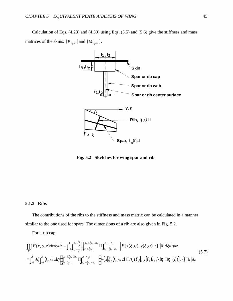
CHAPTER 5 EQUIVALENT PLATE ANALYSIS OF WING 45
Calculation of Eqs. (4.23) and (4.30) using Eqs. (5.5) and (5.6) give the stiffness and mass
matrices of the skins: ][ sparK and ][ sparM .
l l1 2,
h ,h
t ,t
1 2
1 2
Skin
Spar or rib cap
Spar or rib web
Spar or rib center surface
Rib,
Spar,x,
y,
η (ξ)
ξ (η)
r
s
η
ξ
Fig. 3 Wing Spar or Rib
Λ
5.1.3 Ribs
The contributions of the ribs to the stiffness and mass matrix can be calculated in a manner
similar to the one used for spars. The dimensions of a rib are also given in Fig. 5.2.
For a rib cap:
( ) ( )[ ] ( )[ ]{ } dzJzslyslxFdsld
dzddJzyxFdxdydzzyxF
rr
tz
htz
htz
tz
s
l
s
l
htz
tz
tz
htzV
LU
UU
LL
LL
r
r
LU
LL
UU
LU
⋅++
+=
⋅
+=
∫∫ ∫∫
∫ ∫ ∫ ∫∫∫∫−
−−−
++
+−
−
+
−
++
+
−
−−
,)(,,)(,
]),,(),,([),,(
22
1
1 2
1
1
1
1
21
221
221
21
2
2
221
21
21
221
ξηηξξηηξηξ
ηξηξηξη
η (5.7)
Fig. 5.2 Sketches for wing spar and rib

CHAPTER 5 EQUIVALENT PLATE ANALYSIS OF WING 46
where s is the wing span, and )(ξη r is the rib position function.
For the rib web:
( ) ( )[ ] ( )[ ]{ }∫∫∫
∫ ∫ ∫∫∫∫−−
++−−
−
+
−
−−
++
⋅++=
⋅=
221
221
2
2
221
221
,)(,,)(,
]),,(),,([),,(
22
1
1 2
1
1
1
1
htz
htz rr
s
t
s
t
htz
htzV
UU
LL
r
r
UU
LL
dzJzstystxFdstd
dzddJzyxFdxdydzzyxF
ξηηξξηηξηξ
ηξηξηξη
η (5.8)
The same as for the spars, integration on ribs can be obtained by summing up contributions from all
the ribs.
Calculation of Eqs. (4.23) and (4.30) using Eqs. (5.7) and (5.8) give the stiffness and mass
matrices of the skins: ][ ribK and ][ ribM .
5.2 Boundary Conditions
The boundary conditions can be approximated using artificial springs on the boundary.
Applying linear springs with very large magnitudes of stiffness on the boundaries can approximate
the boundary conditions of simply supported edge. Applying linear and rotational springs with very
large magnitudes of stiffness on the boundaries can approximate the boundary conditions of
clamped edge. While details of these practices for a general case can be found in Lovejoy and
Kapania 21,20 , in the following the special case with the wing being clamped at its root will be
treated.
Assume that in Fig. 4.1, there are artificial springs distributed along the side of 12
)1,11( −=≤≤− ηξ . These are linear springs with constant stiff coefficients of xα , yα , zα , xφα ,
and yφα respectively, which are responsive only to displacements of 0u , 0v , 0w , xφ and yφ
respectively. The strain energy that these springs possess can be written as
∫ ++++=12
2220
20
202
1 )( dlwvuU yyxxzyxspring φαφαααα φφ (5.9)

CHAPTER 5 EQUIVALENT PLATE ANALYSIS OF WING 47
Since at side 12 0,2/)}1()1({ 21 =++−= yxxx ξξ , and rcxx == 21 ,0 , here rc is the
chord-length at the root, we have ξξ dcdxxdxdl r21
12 2/)( =−== , therefore Eq. (5.9) becomes
∫−++++=
1
1
2220
20
204
1 )( ξφαφαααα φφ dwvucU yyxxzyxrspring (5.10)
Considering Eqs. (4.9) and (4.11), and comparing Eq. (5.10) with }]{[}{21 qKqU spring
Tspring = ,
we obtain the stiffness matrix for the springs as
])[],[],[],[],([][ yxzyxspring KKKKKdiagK φφααα= (5.11)
where
−−=
−−=
−−=
−−=
−−=
∫∫∫∫∫
−
−
−
−
−
1
121
1
121
1
121
1
121
1
121
)}1,()}{1,({][
)}1,()}{1,({][
)}1,()}{1,({][
)}1,()}{1,({][
)}1,()}{1,({][
ξξξα
ξξξα
ξξξα
ξξξα
ξξξα
φφ
φφ
α
α
α
dBBcK
dBBcK
dBBcK
dBBcK
dBBcK
TRSRSyry
TPQPQxrx
TMNMNzrz
TKLKLyry
TIJIJxrx
(5.12)
The magnitudes of xα , yα , zα , xφα , and yφα must be large enough such that the boundary
conditions are properly simulated. But they cannot be too large, or else all the stiffness values other
than those of these springs will be pushed beyond the significant figures of the computation system.
This is to say, the spring magnitudes need to be within a range in order that the boundary condition
is properly simulated. This range depends on the specifics of the computation environment and the
computer system. In Figs. 5.3 and 5.4 the first 10 natural frequencies of a wing that we shall
specify in 5.4 , obtained using a method to be explained in 5.3 , are shown with regard to the spring
magnitudes. In these cases, it is assumed valueSpringyxzyx ===== φφ ααααα , and 6 and 8
terms of the Lengendre polynomials are used respectively. Since the computation is performed
using MATLAB 5.2, double precision is used. It can seen from both Figs. 5.3 and 5.4 that within the
spring value of 216~8 /(10 inlb or )/ inlb , all of the natural frequencies are stable. In all the
following cases, the spring value will be specified as 1210 .

CHAPTER 5 EQUIVALENT PLATE ANALYSIS OF WING 48
Log10 (Spring value)
W1
,...,W
10
0 5 10 15 200
500
1000
1500
2000
2500
K=6
Fig. 5.3 The first 10 natural frequencies of wing I as functions of boundary-condition-
simulating spring value, when 6 terms of Legendre polynomials are used

CHAPTER 5 EQUIVALENT PLATE ANALYSIS OF WING 49
Log10 (Spring value)
W1,
...,W
10
0 5 10 15 200
500
1000
1500
2000
2500
K=8
Fig. 5.4 The first 10 natural frequencies of wing I as functions of boundary-condition-
simulating spring value, when 8 terms of Legendre polynomials are used

CHAPTER 5 EQUIVALENT PLATE ANALYSIS OF WING 50
5.3 Formulation for Vibration Problem of Wing
Under the assumption that the wing is a conservative system, the Lagrange's equations58 for
free vibration are
0=∂∂−
∂∂
jj q
L
q
L
dt
d�
µν,,1 �=j , .,,,, RSPQMNKLIJ=µν (5.13)
Since the Lagrangian for the wing is
UTVTL −=−= (5.14)
where V is the potential energy, and by using Eqs. (4.22), (4.29) and (5.13), we can find the
natural frequencies and mode shapes for the free vibrating wing by solving the following
eigenvalue problem
[ ] 0}{ =− xMK totaltotal λ (5.15)
where
][][][][],[][][ ribsparskinstrainspringstraintotal KKKKKKK ++=+= , (5.16)
][][][][ ribsparskintotal MMMM ++= , (5.17)
2ωλ = is an eigenvalue of the system of equations, ω is the corresponding frequency in
radians/second, and }{ x is the corresponding eigenvector.
5.4 Convergence Test
Since in Eq. (4.9) only a combination of finite terms of trial functions are used to represent the
deformation of the wing, it is obvious that any results coming from this representation would be an
approximation. This is especially true for the higher modes of the free vibration problem if the
Legendre or Chebyshev polynomials are being employed as the trial functions. The validity of the
method can be established only if the results are converging when more trial function terms are
used. For this purpose, two wings with the following configuration particulars (more details will be
given in 5.6)are used:

CHAPTER 5 EQUIVALENT PLATE ANALYSIS OF WING 51
Wing I: sweep angle $30=Λ , span in192= , chord length at root in72= , chord length at tip
in36= ;
Wing II: sweep angle $891.24=Λ , span in857.72= , chord length at root in627.49= , chord
length at tip in332.24= .
Figs. 5.5 and 5.6 show the first 10 natural frequencies of Wing I and II when 4 to 10 terms of
the Legendre polynomials are used. More cases of convergence tests for plates are reported in
Lovejoy and Kapania 21,20 . We can have the following rule of thumb: when K terms of trial
functions are employed, the first K natural frequencies will have converged or nearly converged
values. Based on this rule, either 6=K or 8=K is used in all calculations in following sections
and chapters.

CHAPTER 5 EQUIVALENT PLATE ANALYSIS OF WING 52
K (Number of Lengendre plynomials)
Nat
ural
frequ
enci
es(r
ad/s
ec)
3 4 5 6 7 8 9 100
1000
2000
3000
4000
N=1N=2N=3N=4N=5N=6N=7N=8N=9N=10
Fig. 5.5 Natural frequencies of wing I with regard to number of trial function terms

CHAPTER 5 EQUIVALENT PLATE ANALYSIS OF WING 53
K (Number of Lengendre plynomials)
Nat
ural
frequ
enci
es(r
ad/s
ec)
3 4 5 6 7 8 9 100
1000
2000
3000
4000
5000
6000
7000
8000
9000
10000
N=1N=2N=3N=4N=5N=6N=7N=8N=9N=10
Fig. 5.6 Natural frequencies of wing II with regard to number of trial function terms

CHAPTER 5 EQUIVALENT PLATE ANALYSIS OF WING 54
5.5 Static Problem Solutions
Assume that an external, distributed force with components ),,( tyxPx , ),,( tyxPy and
),,( tyxPz is applied on the wing structure, then the virtual work done by this load on the
infinitesimal area dydx ⋅ is
zyx QQQQ δδδδ ++= (5.18)
where
dydxtzyxwtyxPQ
dydxtzyxvtyxPQ
dydxtzyxutyxPQ
zz
yy
xx
⋅⋅⋅=⋅⋅⋅=⋅⋅⋅=
),,,(),,(
),,,(),,(
),,,(),,(
δδδδδδ
(5.19)
and by using Eq. (4.1) we obtain
dydxwPQ
dydxzvPQ
dydxzuPQ
zz
yyy
xxx
⋅⋅⋅=⋅⋅⋅+⋅=⋅⋅⋅+⋅=
0
0
0
)(
)(
δδδφδδδφδδ
(5.20)
Using Eq. (4.6), that is, approximating the displacements yxwvu φφ ,,,, 000 in terms of the Ritz
functions, the total work done by the external force on the whole wing surfaces is given by
}{}{
}{}{}{}{
}{}{}{}{}{}{
qP
dxdyBzPBzP
qBPqBPqBPQ
T
yT
RSyxT
PQx
WT
MNzVT
KLyUT
IJx
δ
δφδφ
δδδδ
=
++
++= ∫∫ (5.21)
where }{P is the generalized load vector
TPPPPPP }}{}{}{}{}{{}{ 54321= (5.22)
in which
∫∫∫∫
=
=
dxdyBtyxPzP
dxdyBtyxPP
TRSPQyx
TMNKLIJzyx
}){,,(}{
}){,,(}{
,,5,4
,,,,3,2,1 (5.23)
If the external force is a concentrated force, the above derivations can be simplified. For instance
for the first component of the generalized load vector we have

CHAPTER 5 EQUIVALENT PLATE ANALYSIS OF WING 55
TaaIJaaaax BtyxPP )},(){),,(),,((1 ηξηξηξ= (5.24)
where ),( aa ηξ is the transformed coordinates of the point where the load is applied.
Using the principle of virtual work, we have, for the static case, the following relation for the
generalized displacement vector }{q and generalized load vector }{ P
}{}]{[ PqK = (5.25)
5.6 Results and Discussion
In order to assess the accuracy of the present method and test its performance in various
situations, a series of calculations were carried out for several wing-shaped structures clamped at
the root. Results using MSC/NASTRAN, a commercial finite element code, are provided for
comparison. Finally, for the comparison between the present method and an existing FSDT
method, a swept-back box wing used as a test case in Livne31 were calculated for its free vibration
and static response analyses.
5.6.1 Free Vibration Analysis
5.6.1.1 A Trapezoidal Plate
The geometric and material parameters for the plate are given as: Span=192 inches, Root
width=72 inches, Tip width=36 inches, Sweep angle (leading edge)=$30 , Thickness=1.8 inch
(thickness ration at tip=1/20); Mass Density 424 /sec10526.2 inlb ⋅×= −ρ , Young’s Modulus
27 /10025.1 inlbE ×= , Poisson's Ratio 3.0=ν . The plate is clamped at the root.
Comparisons are made in Fig. 5.7 between the mode shapes as obtained by the present method
and those by the FEA calculations using MSC/NASTRAN employing 200 shell elements
(CQUAD4). The comparison of the natural frequencies is also shown in Fig. 5.7. It can be seen that
both the mode shapes and natural frequencies as obtained using the present method, are in good

CHAPTER 5 EQUIVALENT PLATE ANALYSIS OF WING 56
agreement with those obtained using the FEA. The relative differences of the natural frequencies
for the first 8 modes are within -0.62~2.12%.
by FEA Equivalent Plate Model
Fig. 5.7 Mode Shapes and Natural Frequency f )/( srad for a Trapezoidal Plate

CHAPTER 5 EQUIVALENT PLATE ANALYSIS OF WING 57
5.6.1.2 A Trapezoidal Shell with a Camber
All parameters are the same as with the previous case except that there is a camber with the
camber-chord ratio varying from 2.345% at the root to 0.938% at the tip.
Comparisons are made between the results as obtained by the present method with those
obtained using the FEA in MSC/NASTRAN employing 200 shell elements(CQUAD4), as shown
in Fig. 5.8.
It can be seen that, although this case is very similar to the previous one except for a small
camber, there are significant differences in the natural frequencies of a number of modes. Most of
the variations were predicted quite accurately by the present method, as shown clearly in the
comparison with the FEA results in Fig. 5.8. But the relative differences were slightly higher than
the ones in the previous case, varying in a range of -1.31% to 5.26% for the first 8 modes. Larger
differences for the present case can be attributed to the fact that the present method ignores the
coupling between the in-plane and transverse displacements caused by the mid-surface curvature.

CHAPTER 5 EQUIVALENT PLATE ANALYSIS OF WING 58
by FEA Equivalent Plate Model
Fig. 5.8 Mode Shapes and Natural Frequency f )/( srad
for Wing-Shaped Shell with a Camber

CHAPTER 5 EQUIVALENT PLATE ANALYSIS OF WING 59
5.6.1.3 A Solid Wing
The middle surface of this wing is the same as that of the previous case. Its thickness-chord
ratio is varied from 0.15 at the root to 0.06 at the tip. The sections were generated by the Karman-
Trefftz transformation (see Ref. 59 and Appendix C).
Comparisons are made in Fig. 5.9 between the results as obtained by the present method with
those obtained by the FEA calculations using MSC/NASTRAN employing 250 solid elements
(CHEXA and CPENTA) and 572 nodes. It can be seen that although there are thickness variations
as well as a camber, the present method yields results that compare quite well with those obtained
using the FEA. The relative differences for the first 8 modes were within -5.82~1.42%, comparable
to those in the previous case.

CHAPTER 5 EQUIVALENT PLATE ANALYSIS OF WING 60
by FEA Equivalent Plate Model
Fig. 5.9 Mode Shapes and Natural Frequency f )/( srad for the Solid Wing

CHAPTER 5 EQUIVALENT PLATE ANALYSIS OF WING 61
5.6.1.4 A Built-up Wing Composed of Skins, Spars and Ribs
The outside geometrical shape is the same as in the previous case, the solid wing. There are 4
spars and 10 ribs distributed uniformly in the wing. Sketch of the wing cross-section shapes and rib
and spar positions is shown in Fig. 5.10. Particulars of the wing are: Skin Thickness int 118.0 = ;
Spar Cap Height inh 197.1 = , Spar Cap Width inl 373.1 = , Spar Web Thickness int 058.1 = ; the
ribs have the same cap dimensions and web thickness as the spars.
The FEA calculations are made by using MSC/NASTRAN employing 370 elements and 110
nodes. The wing skins were modeled using shell elements (CQUAD4), the spar and rib caps were
modeled using bar elements (CBAR), and the spar and rib webs were modeled using shear panel
elements (CSHEAR). Comparison between the mode shapes as well as the corresponding natural
frequencies as obtained by the two methods are shown in Fig. 5.11. It can be seen that the mode
shapes were simulated equally well by the present method as compared to the FEA, and it is found
that the relative differences for the first 8 modes were within -4.79~2.15 %, comparable to those in
the previous cases.

CHAPTER 5 EQUIVALENT PLATE ANALYSIS OF WING 62
X Y
Z
Fig. 5.10 Wing cross-sections at rib positions and spar positions

CHAPTER 5 EQUIVALENT PLATE ANALYSIS OF WING 63
by FEA Equivalent Plate Model
Fig. 5.11 Mode Shapes and Natural Frequency f )/( srad
for a Built-up Wing Composed of Skins, Spars and Ribs

CHAPTER 5 EQUIVALENT PLATE ANALYSIS OF WING 64
5.6.1.5 A Box Wing used as a test case in Livne21 .
This is a cantilevered all aluminum wing swept back by $30 . It has a constant thickness and
constant chord length. Its 5 spars and 3 ribs with identical cross sections are bonded to the top and
bottom cover skins (see Fig. 5.12). Details of this box wing can be found in Refs. 31 and 60. The
same kinds of elements were employed as in the previous case. Results for the natural frequencies
by the FEA using MSC/NASTRAN and the present FSDT are shown in Table 5.1, in comparison
with those given in Livne31 by the FEA using ELFINI and a FSDT based on simple-polynomial
trial functions. While there are some differences between the two FEA calculations, which may
have been caused by different discretization and element choices, the accuracy of the present FSDT
results are promising.
Fig. 5.12 A box wing
Table 5.1 Natural frequencies (Hz) of the cantilevered swept-back box wing
Mode No.
Description ofMode Shape
FEA(Livne31)
FSDT(Livne31)
FEA(present)
FSDT(present)
1 1st bending 115.6 114.7 116.6 118.02 In plane 317.6 312.4 327.9 349.73 1st torsion 418.4 428.9 409.4 419.14 2nd bending 576.4 575.3 572.1 571.15 2nd torsion 1086 1125 1064 1090

CHAPTER 5 EQUIVALENT PLATE ANALYSIS OF WING 65
5.6.2 Displacement under Static Loads
The built-up wing in the 4-th case (5.4.1.4) of the free vibration analysis is used here. Three
cases of static load were considered as shown as follows.
5.6.2.1 Tip Point Force
A downward (-z-direction) force of magnitude of 1lb is applied at the middle point of the
wing tip. The displacements along the leading and trailing edge of the wing are shown in Fig. 5.13.
It can be seen that the present method calculated the vertical displacement w accurately compared
with the FEA, and also predicted quite well the trends of variation for the other two displacement
components, u and v .
5.6.2.2 A Force Distribution
A downward (-z-direction) force of magnitude of 1lb is applied at every upper-surface nodes
of the FEA model. This is a case similar to the wing being under uniform pressure difference
between its upper and lower surfaces. The displacements along the leading and trailing edge of the
wing are shown in Fig. 5.14. Quite similar results to those in load case 5.4.1.2 were obtained.
5.6.2.3 Tip Torque
A downward (-z-direction) force of magnitude of 1lb is applied at the tip of the fore-most
spar, while an upward (z-direction) force of magnitude of 1lb is applied at the tip of the aft-most
spar. This is a case in which the wing tip is subjected to a torque. The displacements along the
leading and trailing edges of the wing are shown in Fig. 5.15. The relative difference for w at the
tip/leading-edge corner and tip/trailing-edge corner are 26.4% and 2.64% respectively. Note that
the absolute differences are 410397.0 −× inch and 410181.0 −× inch respectively; therefore the large
relative difference at the tip/leading-edge corner is because of the small magnitude of w along the
leading edge, and the difference between the twist angles predicted by the two methods would be
small.

CHAPTER 5 EQUIVALENT PLATE ANALYSIS OF WING 66
Y (inch)
100
u,10
0v,w
(inch
)
0 50 100 150-3
-2.5
-2
-1.5
-1
-0.5
0
0.5
100u(FEM)100v(FEM)w(FEM)100u(present cal.)100v(present cal.)w(present cal.)
x 10-3
(a) leading edge
Y (inch)
10
0u,
10
0v,
w(in
ch)
0 50 100 150-3.5
-3
-2.5
-2
-1.5
-1
-0.5
0
0.5
100u(FEM)100v(FEM)w(FEM)100u(present cal.)100v(present cal.)w(present cal.)
x 10-3
(b) trailing edge
Fig. 5.13 Comparison of Displacements for Load Case of Tip Point Force

CHAPTER 5 EQUIVALENT PLATE ANALYSIS OF WING 67
Y (inch)
100u
,100
v,w
(inch
)
0 50 100 150-0.06
-0.05
-0.04
-0.03
-0.02
-0.01
0
0.01
100u(FEM)100v(FEM)w(FEM)100u(present cal.)100v(present cal.)w(present cal.)
(a) leading edge
Y (inch)
100
u,10
0v,
w(in
ch)
0 50 100 150-0.07
-0.06
-0.05
-0.04
-0.03
-0.02
-0.01
0
0.01
100u(FEM)100v(FEM)w(FEM)100u(present cal.)100v(present cal.)w(present cal.)
(b) trailing edge
Fig. 5.14 Comparison of Displacements for Load Case of a Force Distribution

CHAPTER 5 EQUIVALENT PLATE ANALYSIS OF WING 68
Y (inch)
100
u,10
0v,w
(inch
)
0 50 100 150-5
0
5
10
15
20
100u(FEM)100v(FEM)w(FEM)100u(present cal.)100v(present cal.)w(present cal.)
x 10-5
(a) leading edge
Y (inch)
100u
,100
v,w
(inch
)
0 50 100 150-1
0
1
2
3
4
5
6
7
8
100u(FEM)100v(FEM)w(FEM)100u(present cal.)100v(present cal.)w(present cal.)
x 10-4
(b) trailing edge
Fig. 5.15 Comparison of Displacements for Load Case of Tip Torque

CHAPTER 5 EQUIVALENT PLATE ANALYSIS OF WING 69
5.6.2.4 The Box Wing in Livne21
The swept-back box wing is under a downward point force of 1lb at the tip of the rear spar.
Displacements at the wing tip from measurement, FEA calculation and present method are shown
in Table 5.2. It can be seen that the present method yielded very good results for this test case.
Table 5.2 Displacement (in) of the cantilevered swept-back box wing
Position Measured 60,31 FEA(present) FSDT(present)Front spar tip 41081.1 −× 41079.1 −× 41074.1 −×Rear spar tip 41021.2 −× 41019.2 −× 41020.2 −×
5.6.3 Skin Stress Distributions
The upper and lower skin stress of the wing in the above static case (5.4.2.1) were calculated
using the present method. The Von Mises stress distribution along a line with a distance of 5% span
to the root chord is shown in Fig. 5.16(a) in comparison with points obtained using
MSC/NASTRAN. Also the Von Mises stress distribution along a span-wise line with a distance of
37.5% chord length to the leading edge is shown in Fig. 5.16(b) in comparison with points obtained
using MSC/NASTRAN. It can be seen that, although there are substantial differences (the largest
one is about 15%) between the present calculations and the stresses determined using the FEA, the
variation trends of the stresses from both methods are quite similar. This means that the position of
the largest stress determined by the present method will be reliable. The Von Mises stress
distributions on the upper and lower skins calculated using the present method are shown in Figs.
5.17 and 5.18 respectively.

CHAPTER 5 EQUIVALENT PLATE ANALYSIS OF WING 70
Relative Distance to Leading-Edge
Von
Mis
esS
tress
(psi
.)
0 0.25 0.5 0.75 10
1
2
3
4
5
Lower Skin (FEM)Upper Skin (FEM)Lower Skin (present cal.)Upper Skin (present cal.)
(a) Near the Root Chord
Relative Distance to Wing Root
Von
Mis
esS
tress
(psi
.)
0 0.25 0.5 0.75 10
1
2
3
4
5
6
Lower Skin (FEM)Upper Skin (FEM)Lower Skin (present cal.)Upper Skin (present cal.)
(b) Near the Central Spar
Fig. 5.16 Comparison of Von Mises Stress on the Upper and Lower Skins
of a Wing under a Point Force at the Wing Tip

CHAPTER 5 EQUIVALENT PLATE ANALYSIS OF WING 71
0
2
4
6
Von
Mis
esst
ress
(psi
)
0
0.2
0.4
0.6
0.8
1 Relative dist ance to the root
0
0.2
0.4
0.6
0.8
1
Relative dist ance to leading-edge
0.85
5.04
0.50
3.65
3.65
2.25
2.95
4.70
2.252.95
3.65
2.60
3.30
0.85
4.704.70
3.65
4.35
2.60 2.60
2.25
1.55
0.50
X Y
Z
Von Mises Stress on Upper skin
Fig. 5.17 Distribution of Von Mises Stress on the Upper Skin
of a Wing under a Point Force at the Wing Tip

CHAPTER 5 EQUIVALENT PLATE ANALYSIS OF WING 72
0
2
4
6
Von
Mis
esst
ress
(psi
)
0
0.2
0.4
0.6
0.8
1 Relative dist ance to the root
0
0.2
0.4
0.6
0.8
1
Relative dist ance to leading-edge
4.00
2.95
4.35
1.90
2.953.30
1.90
1.551.20
1.90
X Y
Z
Von Mises Stress on Lower Skin
Fig. 5.18 Distribution of Von Mises Stress on the Lower Skin
of a Wing under a Point Force at the Wing Tip

CHAPTER 5 EQUIVALENT PLATE ANALYSIS OF WING 73
5.6.3 On Efficiency of EPA
To show the efficiency of the present equivalent plate analysis of built-up wings, the ideal
situation would be comparison of the CPU times used in EPA and other analysis methods, such as
FEA. But it seems to the author that only under the following situations the comparison can be
made meaningful: (1) The two calculations are to be carried out in the same computing
environment to exclude the difference that different environments may cause, that is to say, both
should be coded using the same language, such as in FORTRAN or the MATLAB m file; (2) Similar
linear algebraic solvers and other type of supplementary algorithms, be used. Unfortunately, the
author could not establish a comparison based upon such requirements. While the EPA was coded
in the MATLAB m file, the FEA was carried out using a commercial package, MSC/NASTRAN.
But we still can perform a comparison of efficiency in an indirect way, that is, by comparing
the number of degrees of freedom (DOF), and elements used. DOF determines the dimensions of
the stiffness and mass matrices, therefore directly influences the CPU time required to solve a static
or dynamic problem through operations upon these matrices. The number of elements, on the other
hand, represents the effort needed to set up element matrices and assemble them together to create
the global matrices. For the case of EPA, the number of elements can be deemed as k2.
Details of DOF and number of elements for several of the previous example cases are displayed
in Table 5.3. As shown in Table 5.3, for these simple cases, the FEA uses thousands or hundreds of
DOF, while for the EPA it is always 180 or 360, depending on whether 6 or 8 terms of polynomials
are used. That means a very big difference on computational effort for either static or dynamic
problems, if the same linear algebraic solvers are used. However, in reality the more efficient
sparse matrix solvers can be used for FEA, therefore the difference of efficiency would not be a
direct comparison of the DOFs.
Similar situation is shown for the comparison of numbers of elements in Table 5.3. Still we
cannot say that the ratio of the computational effort for the element matrix terms for FEA and EPA
is the ratio of the numbers of elements, because for EPA the elements are global, and more effort is

CHAPTER 5 EQUIVALENT PLATE ANALYSIS OF WING 74
needed for calculating the element matrices. It is based on this reasoning that a more efficient
approach is pursued in Chapter 7.
It is worth noting that for the FEA of the built-up wing the ratio of number of elements to DOF
is the largest, more than 3 times higher than the other cases. This indicates a relative larger
computational effort on calculating and assembling the element matrices in the FEA, also more
efforts for calculating the contributions from the structure components in the EPA. Therefore it
seems that the difference in efficiency of FEA and EPA is more reliably reflected in the difference
between the DOFs.
Table 5.3 Comparison of FEA and EPA in terms of DOF and Number of Elements
FEA EPAExample
DOF
No. ofElements
DOF
k=6DOF
k=8No. of
Elementsk=6
No. ofElements
k=8
Trapezoidal plate & shell 1350 200 180 320 36 64
Solid wing 3300 250 180 320 36 64
Built-up wing 600 370 180 320 36 64

75
Chapter 6
Modal Response Using Sensitivity Techniques
and Direct Application of Neural Networks
The modal response of wing structures is very important for assessing their dynamic response
including dynamic aeroelastic instabilities. Moreover, in a recent study61 an efficient structural
optimization approach was developed using structural modes to represent the static aeroelastic
wing response (both displacements and stresses).
In this chapter, the natural frequencies of general trapezoidal wing structures are to be
approximated using shape sensitivities up to the 2nd order, and different approaches of computing
the derivatives are investigated. The baseline design and shape sensitivities are calculated based on
the equivalent plate-model analysis (EPA) method developed by Chapter 4 and 5. For
comparison, an efficient method that employs the artificial neural networks to relate the natural
frequencies of a wing to its shape variables is also established. An example of a 34 full factorial
experimental design, i.e., 4 levels in 3 variables, is treated by these methods to display their
respective merits.
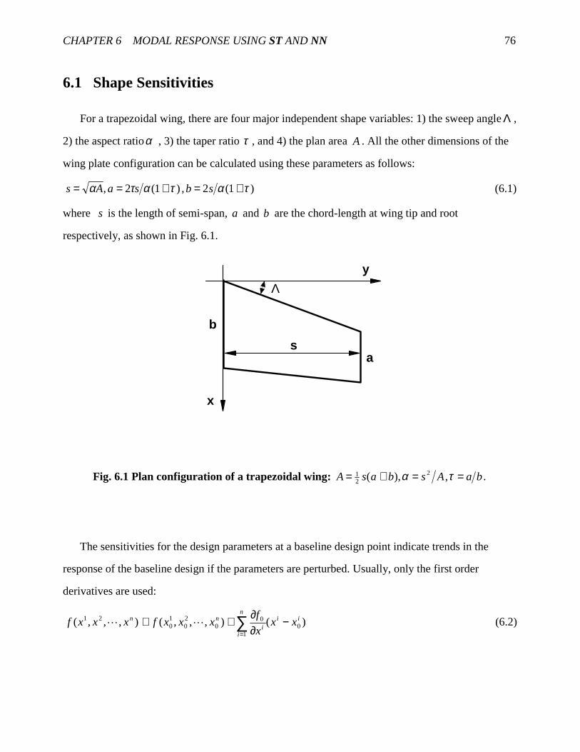
CHAPTER 6 MODAL RESPONSE USING ST AND NN 76
6.1 Shape Sensitivities
For a trapezoidal wing, there are four major independent shape variables: 1) the sweep angleΛ ,
2) the aspect ratioα , 3) the taper ratio τ , and 4) the plan area A . All the other dimensions of the
wing plate configuration can be calculated using these parameters as follows:
)1(2,)1(2, τατατα +=+== sbsaAs (6.1)
where s is the length of semi-span, a and b are the chord-length at wing tip and root
respectively, as shown in Fig. 6.1.
x
y
sa
b
Λ
Fig. 6.1 Plan configuration of a trapezoidal wing: .,),( 221 baAsbasA ==+= τα
The sensitivities for the design parameters at a baseline design point indicate trends in the
response of the baseline design if the parameters are perturbed. Usually, only the first order
derivatives are used:
)(),,,(),,,( 01
00
20
10
21 iin
ii
nn xxx
fxxxfxxxf −
∂∂+≅ ∑
=
�� (6.2)

CHAPTER 6 MODAL RESPONSE USING ST AND NN 77
where ),,,(
0
020
10
nxxxii x
f
x
f
�
∂∂=
∂∂
is the sensitivity at the baseline point with respect to the i -th design
parameter. For a more accurate approximation, we can use higher-order derivatives in the Taylor’s
expression:
),,,()(
),,,()(),,,(),,,(
020
10
2
102
1
10
20
1000
20
10
21
nn
ii
ii
n
i
ni
iinn
xxxfx
xx
xxxfx
xxxxxfxxxf
�
���
∂∂−+
∂∂−+≅
∑
∑
=
= (6.3)
where besides the first order derivatives, second order derivatives ),1,(02
njixx
fji
�=∂∂
∂ are also
used.
6.2 An Issue in Equivalent Plate Analysis (EPA)
Due to its efficiency in determining the natural frequencies and mode shapes of wings, the
Equivalent Plate Analysis (EPA) described in Chapters 4 and 5 can be used to investigate the
variation of modal response, that is, to evaluate the sensitivities of the natural frequencies with
respect to trapezoidal wing structures shape changes. For determining the response of the baseline
design, the EPA can be used, or the FEA employing a commercial package such as
MSC/NASTRAN can be used for better accuracy.
A key problem that needs to be addressed before this evaluation can be made is mode tracking.
The natural frequencies given by an ordinary eigenvalue solver are usually ranked by magnitude
but not by the modal content. As design variables are perturbed, frequencies drift and mode
crossing may occur. An algorithm for mode tracking is needed to maintain the correspondence
between eigenpairs of the baseline and the perturbed design. Several methods for such purpose
have been given by Eldred et al for self-adjoint62 and nonself-adjoint63 eigenvalue problems.
CHAPTER 6 MODAL RESPONSE USING ST AND NN 78
In the present study, a simple yet effective method is used. In this method, any ordinary
eigenvalue solver can be used, and the modes of the baseline structure are chosen as the
benchmarks. By using the modal assurance criterion (MAC) defined as
}){}})({{}({
}){}({ 2
iT
ijT
j
iT
jjiMAC
φφφφφφ
= (6.4)
where }{ jφ and }{ iφ are the eigenvector for the perturbed and the baseline design respectively, if
)(max lil
ji MACMAC = , we say that the j -th mode of the perturbed design corresponds to the i -th
mode of the baseline structure.
6.3 Approaches to Sensitivity Evaluation
There can be three kinds of approach for obtaining sensitivity derivatives: the finite difference
approach, the analytical approach, and the semi-analytical approaches. The finite difference
approach is very simple to formulate and implement, but is numerically inefficient and is sensitive
to the step-size used. A too-large step size usually causes significant truncation errors and a too-
small step size may lead to large round-off errors. As a result, the more elegant and accurate
analytical approach is used if it does not involve complex mathematical derivation. But for most
practical problems, the derivation of analytical derivatives is too formidable to handle manually.
The basic idea behind the Automatic Differentiation (AD) is to let a computer to perform such
extensive tasks. The advantage of AD is to avoid truncation errors. The method has found
applications in sensitivity evaluation42,41 . For the basic theory of AD one can consult Ref. 64, and
for the state-of-the-art of AD one can refer to Ref. 65. If an approach uses both analytical and
finite-difference solutions to obtain the derivative, then it can be called a semi-analytical one.
The finite difference approaches can be constructed using the following formulas:
)(2
)()()( 2xO
x
xxfxxfxf ∆+
∆∆−−∆+=′ (6.5)

CHAPTER 6 MODAL RESPONSE USING ST AND NN 79
)()()(2)(
)( 2
2xO
x
xxfxfxxfxf ∆+
∆∆−+−∆+=′′ (6.6)
where
xx ⋅=∆ ε (6.7)
in which ε is the relative step size, but herein it is simply called the step size. Eq. (6.5) can be
applied twice for evaluating the mixed second order derivatives such as )(02
jixx
fji
≠∂∂
∂.
The analytical approaches for shape sensitivities of modal response can be based on the
following equations
}{][][
}{ iiT
ii MK φ
θλ
θφ
θλ
∂∂−
∂∂=
∂∂
(6.8)
∑=
=∂
∂ n
jjij
i
1
}{}{
φαθφ
(6.9)
where
∂∂−=
≠
∂∂−
∂∂
−=
}{][
}{2
1
},{][][
}{)(
1
iT
iii
iiT
iji
ij
M
ijMK
φθ
φα
φθ
λθ
φλλ
α (6.10)
here θ is the shape variable, iλ and }{ iφ are the i -th eigenvalue and eigenvetor, and }{ iφ is mass-
normalized such that 1}]{[}{ =iT
i M φφ . Eqs. (6.8) and (6.9) were first derived by Wittrick66 and
Fox and Kapoor67 respectively. One can find more on this topic in Ref. 68.
The major difficulty of applying Eqs. (6.8) and (6.9) lies in the calculation of θ∂
∂ ][ K and
θ∂∂ ][ M
. For instance, consider θ∂
∂ ][ K. According to Chapter 4, the stiffness matrix ][K is
formulated as an integral

CHAPTER 6 MODAL RESPONSE USING ST AND NN 80
ηξ
ηξ
ddCGC
ddCdzJTDTCdVCTDTCK
T
z
z
TT
V
TT
][][][
][][][][][]][][[][][][
1
1
1
1
1
1
1
1
2
1
∫ ∫
∫ ∫ ∫∫∫∫
− −
− −
=
==
(6.11)
where only the inner part dzJTDTGz
z
T ][][][][2
1∫= is a function of the shape variables, and the
Gaussian quadrature is used to obtain the integration on ξ and η . Therefore,
ηξθθ
ddCG
CK T ][
][][
][ 1
1
1
1∫ ∫− −
∂∂=
∂∂
(6.12)
in which θ∂
∂ ][Gcan either be determined analytically or numerically.
People often make use of the advantages of both the finite difference and analytical approaches
in different stages of obtaining some complicated sensitivities. While trying to use the analytical
approach as much as possible, in other parts of the process the finite difference is used, as in the
cases of Refs. 40 and 42. This kind of approach is usually called semi-analytical.
In summary, there are three approaches to calculate the first order modal sensitivities:
(i) analytical approach: Eqs.(6.8)~(6.10) are used, and θ∂
∂ ][ K and
θ∂∂ ][ M
are determined
analytically.
(ii) semi-analytical approach: Sensitivities θ∂
∂ ][K and
θ∂∂ ][M
in Eqs.(6.8)~(6.10) are
determined numerically, that is, for the case of θ∂
∂ ][K, Eq. (6.12) is used where
θ∂∂ ][G
is calculated
using a finite difference scheme.
(iii) finite difference approach: θλ
∂∂ i and
θφ
∂∂ }{ i are determined using Eq. (6.5) directly.
For the second order sensitivities, there can still be three approaches as specified above. While
the formulation for the analytical approaches is becoming more complicated, a scheme as simple as
Eq. (6.6) can be used for the finite difference approach.

CHAPTER 6 MODAL RESPONSE USING ST AND NN 81
6.4 Application of Sensitivity Technique (ST) in Multi-variable
Optimization
In a multi-variable case, the following formulation is used instead of Eq. (6.3):
RR
RR TTi
2
)(2
1)()()(
∂∂−+
∂∂−+≅
ii
iii p
ppp
pppp (6.13)
where Tnvvv ),,,( 21�=p is an arbitrary point in the design space, Tn
iii vvv ),,,( 21�=ip is the i -
th node point in the design space, )( piR is the response at p estimated by using the response and
its sensitivities at ip , )( ipR is the response at the i -th node point ip , and
ippip
=
∂∂
∂∂
∂∂=
∂∂
T
nvvv,,, 21 � .
Once there are enough estimates for the response at p using Eq. (6.13), a more accurate
evaluation of response at p can be determined using the following weighting procedure involving
the so-called exponentially decaying influence function35 :
∑=i
ii RwR )()()( ppp (6.14)
where i ranges through the wN design points which are closest to p , and the weight coefficients
)( piw are determined such that its sum is unity:
∑ −−−−
=
ip
pi C
Cw
)exp(
)exp()(
i
i
pp
ppp (6.15)
in which pC is an empirical constant, and the distance between p and ip is defined as
∑=
−=−n
j
ji
j vv1
2)(ipp . It can be seen that 1)( =∑i
iw p .

CHAPTER 6 MODAL RESPONSE USING ST AND NN 82
6.5 Application of Neural Networks (NN)
In this case, the input layer includes all the design variables of interest (for instance, the four
shape parameters of the wing plan form). The output layer gives the desired structural responses,
such as natural frequencies etc. The EPA is being used as the training data generator, though if
necessary, results obtained using FEM can also be used as the training data. Preparation of training
data is very important, and the training algorithm used also greatly impacts the training process23 .
Caution must be exerted in specifying the network parameters and training criterion so that the
results of the trained network would not oscillate around the training data. The direct application is
what we do in this paper.
6.6 Examples and Discussion
6.6.1 Results on sensitivity evaluation
Particulars of the baseline wing structure are as follows: the sweep angle $30=Λ , the aspect
ratio 5.3=α , the taper ratio 5.0=τ , the plan area 25832inA = . The wing sections are generated
using the Karman-Trefftz transformation (Ref. 59, and details in Appendix C) and has a thickness-
chord ratio of 0.15 at the wing root and 0.06 at the tip. The skin thickness int 118.0 = . There are 4
spars and 10 ribs distributed uniformly under the skins. Particulars of the spars and ribs are the
same: the cap height inh 197.1 = , the cap width inl 373.1 = , and the web thickness int 059.1 = .
There is only one material used with mass density 424 /sec10526.2 inlb ⋅×= −ρ , Young’s modulus
27 /10025.1 inlbE ×= , and Poisson's ratio 3.0=ν . The wing is clamped at the root.
An example of using EPA to calculate the natural frequencies with regard to shape variables
while tracking modes by evaluating MACs is provided in Fig. 6.2, where the variation of the
natural frequencies of the first 10 modes w.r.t. the aspect ratio are shown. It can be seen that for
most cases the intersection of natural frequencies has been treated well, and only in a few cases the
frequency variations near the intersection point seem to have a minor problem, probably due to

CHAPTER 6 MODAL RESPONSE USING ST AND NN 83
some kind of interaction between the two modes. If an eigenvalue solver that can work more
accurately with repeated eigenvalues is made use of, the situation can be improved.
The effect of step size on the finite difference approach for sensitivities was investigated for all
the four shape variables. The case with the taper ratio is shown in Fig. 6.3. From all the cases, it is
seen that for the best results for both the 1st and 2nd order sensitivities, the step size ε defined in
Eq. (6.7), should be between 0.005~0.015, and for fairly accurate results ε can be between
0.0017~0.045.
To evaluate θ∂
∂ ][ G analytically proved to be formidable except only in some simplified cases.
In order to compare the sensitivities using the analytical, semi-analytical and finite difference
approach, a special case of the above baseline wing with a constant thickness was considered so
that the analytical derivation of θ∂
∂ ][G in Eq. (6.12) is not formidable. When ε is specified as
0.005, it is found that for the 1st order sensitivities to the four shape variables ( ,,, ταΛ and A ) the
relative difference (averaged for the first 10 modes) between the finite difference and analytical
approach is 0.003%, 0.003%, 0.002% and 0.003% respectively. The relative difference between the
semi-analytical and analytical approach is 0.14%, 0.04%, 0.02% and 0.01% respectively. Therefore
in this case the finite difference approach is more accurate than the semi-analytical one, however
both the approaches yield quite accurate results.

CHAPTER 6 MODAL RESPONSE USING ST AND NN 84
Aspect Ratio
Nat
ural
Fre
quen
cies
(rad
/sec
)
2 3 4 50
500
1000
1500
2000
2500
3000
3500
Fig. 6.2 Natural frequencies using equivalent plate analysis with mode tracking

CHAPTER 6 MODAL RESPONSE USING ST AND NN 85
Log (step size)
Sen
sitiv
ities
-4 -3 -2 -1-3000
-2500
-2000
-1500
-1000
-500
0
500
1000
1500
2000
1st Order(2nd Order)/200
10
step size =0.005-0.015
step size =0.0017-0.045
Fig. 6.3 Effect of the finite difference step size on the sensitivities
of various natural frequencies to taper ratio

CHAPTER 6 MODAL RESPONSE USING ST AND NN 86
For the original baseline wing, since the derivation of the analytical derivatives for θ∂
∂ ][G is
too formidable, only the comparison of the 1st order sensitivities using the finite difference and the
semi-analytical approach was made. It is found in this case the sensitivities to the aspect ratioα ,
taper ratio τ and plan area A using both approaches are quite close, the average difference for the
first 10 modes being in the range of 0.5~1.4%. As an example, the 2nd natural frequency w.r.t. A is
shown in Fig. 6.4, where it can be seen that the 1st order sensitivities using the finite difference and
the semi-analytical approach almost coincide with each other. On the other hand, sensitivities to the
sweep angle Λ using the two approaches have had some quite large relative differences especially
for modes whose sensitivity to Λ is small. One such example, the 3rd natural frequency w.r.t. Λ , is
shown in Fig. 6.5, where attention should be paid to the scale for the vertical coordinate to see how
small the sensitivity to Λ is.
It is observed in Fig. 6.5 that, as in the case of the constant-thickness wing, the finite difference
approach has a better performance than the semi-analytical one. In fact, in some extreme cases, the
linear approximation using the first order sensitivity obtained using the semi-analytical approach is
not at all tangent to the actual variation at the baseline point. This is not the case for that using the
finite difference approach, if the step size chosen is not too large. However, the computational
effort for the semi-analytical approach might be less than that for the finite difference approach,
since in the former case the eigenvalue problem needs to be solved only once while in the latter it
needs to be solved twice.

CHAPTER 6 MODAL RESPONSE USING ST AND NN 87
Plane Area (in )
Nat
ural
Fre
quen
cy(r
ad/s
ec)
4500 5000 5500 6000 6500 7000600
620
640
660
680
700
720
740
760
780
Actutal VariationLinear Approx. (fd)2nd-Order Approx.Linear Approx. (semi-an)
2
Bas
elin
e
Fig. 6.4 The 2nd natural frequency w.r.t. wing plan area
using 1st and 2nd order sensitivities

CHAPTER 6 MODAL RESPONSE USING ST AND NN 88
Sweep Angle (deg)
Nat
ural
Fre
quen
cy(r
ad/s
ec)
25 30 35766
767
768
769
770
771
772
773
774
775
776
Actual VariationLinear Approx. (fd)2nd-Order Approx.Linear Approx. (semi-an)
Bas
elin
e
Fig. 6.5 The 3rd natural frequency w.r.t. wing sweep angle
using 1st and 2nd order sensitivities

CHAPTER 6 MODAL RESPONSE USING ST AND NN 89
It is obvious from observing Figs. 6.4 and 6.5 that the approximation using sensitivities up to
the second order has much improved the results compared with the case where only the first order
sensitivity is used. Similarly it has been shown in Haftka and Gurdal69 that, for the stress-ratio in a
three-bar truss, the quadratic approximation is much more accurate than the linear one. Also it can
be seen that the second order sensitivities using the finite difference scheme of Eq. (6.6) are fairly
accurate, at least for the purpose of engineering application. Another advantage of this scheme is
that it shares the perturbation data with the first order sensitivity scheme Eq. (6.5), therefore its
evaluation has no increase in the computational effort at all.
Using the finite difference approach based on Eq. (6.5) the mixed second order sensitivities
)(02
jixx
fji
≠∂∂
∂can be readily determined. As an example, the mixed second order sensitivity on τ
and A for the first five natural frequencies were calculated, and the results are listed as follows:
0.0099, 0.0153, 0.0353, 0.0494 and 0.0156.
6.6.2 Application of Sensitivity Technique (ST) and Neural Networks (NN)
For a trapezoidal wing, there are four major independent shape variables, i.e. the sweep angle
Λ , the aspect ratio α , the taper ratio τ , and the plan area A . As an example , a 34 full factorial
experimental design with 4 levels in α,Λ , and τ respectively, was used. Particulars of the levels
of every variable are as follows: ]30,20,10,0[ $$$$=Λ , ]5.2,0.2,5.1,0.1[=α , and
]6.0,5.0,4.0,3.0[=τ . The plan area is chosen to be a constant: 23500inA = . The other particulars
are the same as in 6.7.1.
The natural frequencies of the wing structure at the 64 node points in the design space were
calculated using EPA, and the 1st and 2nd order sensitivities at these points were also determined by
finite difference using EPA3. For each mode, a feed-forward neural network with a structure of
110153 ××× , i.e. 3 inputs, 15 neurons in the first hidden layer, 10 neurons in the second hidden
layer, and 1 output, is trained using the MATLAB NN Toolbox function trainlm that trains feed-
forward network with the Levenberg-Marquardt algorithm8 . There are 64 sets of training data,

CHAPTER 6 MODAL RESPONSE USING ST AND NN 90
which are non-dimensionalized before the training process. Once the networks are trained, the
input-output relationships can be readily retrieved by using the function simuff.
For the application of sensitivity technique, the major task is to evaluate the sensitivities, and
to generate responses at an arbitrary design point using Eqs. (6.13) and (6.14) does not need large
amount of CPU time. The constantpC in Eq. (6.14) was specified to be 10, and 10=wN was used.
Shown in Fig. 6.6 are the first 6 natural frequencies of 20 randomly chosen wing structures
inside the box defined in terms of lower and upper bounds on the design variables specified above.
From the figure it can be seen that both of the results given by NN and ST are in very good
agreement with the desired values (those given by the EPA) except for a few cases where there are
some differences. These cases might be caused by the unstable performance of the algorithm used
for extracting eigenvalues in the EPA near the mode-crossing points, as shall be shown in Figs 6.7
and 6.8. In order to see the effects of sensitivity order, a randomly chosen path inside the design
space box is defined as
−==
==Λ=
=+−=
).1/(,
,,,
3,2,1,)1(321
10
jjj
nj
jjjjj
rrnsa
vvv
javavv
j
τα (6.16)
where jv0 and jv1 are lower and upper bounds of variable jv , for instance, $010 =v , $301
1 =v etc.,
]1,0[∈s is the range of a shape variable, and )3,2,1( =jr j are randomly determined values between
0 and 1. Results of natural frequencies of the first 4 modes for wing structures defined by points
along a path with n1=0.945, n2 =8.200, and n3=3.203 are shown in Fig. 6.7, where only the 1st
order sensitivities were used, and in Fig. 6.8, where sensitivities up to the 2nd order were used. It
can be seen that when sensitivities up to the 2nd order are used, results are effectively improved.
Generally speaking, neural networks and sensitivity technique can give equally good results,
and the former uses less time than the latter. But both methods, once the NNs are trained or the
sensitivities are obtained, are much more efficient than the EPA . For instance, the CPU times

CHAPTER 6 MODAL RESPONSE USING ST AND NN 91
consumed by the EPA, the sensitivity based method and the NN based method are in the ratio of
06.0:1:55 .
The example used above has only three variables. For design problems with more variables, the
method of NN and ST can still be applied in general, only at the expense of more computing time.
We can expect that similar conclusions to those obtained above still apply to these cases. For a
design problem with very large number of variables, in combination with the NN or ST method,
methodologies to shrink the design space, such as the reasonable design space approach described
in Balabanov et al70 , can be used. This can make the search of optimal design easier and at the
same time the application of NN or ST more accurate, just as the case in Ref. 26 where the
response surface approximation was used to simulate high-fidelity models. Also for this kind of
high dimensionality design problems, a full multi-level factorial experimental design is almost
impossible to use hence the methods of either NN, or ST, or even response surface are hard to
apply because the cost would be too high. In such a case, an incomplete block statistical
experimental design using the D-optimal criterion72,71 can be used, which, with much reduced
number of design node points, makes the application of NN or ST possible.

CHAPTER 6 MODAL RESPONSE USING ST AND NN 92
Frequencies by EPA (rad/sec)
Sim
ulat
edF
requ
enci
es(r
ad/s
ec)
0 1000 2000 3000 40000
500
1000
1500
2000
2500
3000
3500
4000
by Neural Networksby Sensitivity Technique
Fig. 6.6 Comparison of the natural frequencies of the first 6 modes for wing structures
randomly chosen inside the box of design space, as obtained by the NN and ST
w.r.t. those obtained using a full-fledged EPA

CHAPTER 6 MODAL RESPONSE USING ST AND NN 93
+ + + + + + + + + + + + + + + + + + + + + + + + + + + + + + + + + + + + + + + + + + + + + + + + + +
Shape Variable Range
Sim
ulat
edF
requ
enci
es(r
ad/s
ec)
0 0.25 0.5 0.75 10
500
1000
1500
2000
2500
3000
3500
4000 by EPAby Neural Networksby ST, 1st modeby ST, 2nd modeby ST, 3rd modeby ST, 4th mode
+
0 0.25 0.5 0.75 10
500
1000
1500
2000
2500
3000
3500
4000
Fig. 6.7 Comparison of the natural frequencies of the first 4 modes for wing structures
along a path inside the box of design space (n1=0.945, n2 =8.200, n3=3.203)
using only the 1st order sensitivities

CHAPTER 6 MODAL RESPONSE USING ST AND NN 94
+ + + + + + + + + + + + + + + + + + + + + + + + + + + + + + + + + + + + + + + + + + + + + + + + + +
0 0.25 0.5 0.75 10
500
1000
1500
2000
2500
3000
3500
4000 by EPAby Neural Networksby ST, 1st modeby ST, 2nd modeby ST, 3rd modeby ST, 4th mode
+
Shape Variable Range
Sim
ulat
edF
requ
enci
es(r
ad/s
ec)
0 0.25 0.5 0.75 10
500
1000
1500
2000
2500
3000
3500
4000
Fig. 6.8 Comparison of the natural frequencies of the first 4 modes for wing structures
along a path inside the box of design space (n1=0.945, n2 =8.200, n3=3.203)
using sensitivities up to the 2nd order

95
Chapter 7
Equivalent Skin Analysis Using Neural
Networks
Since the calculation of various integrals in Eqs. (4.23) and (4.30) are time-consuming, it is desired
to replace the actual wing structure by an equivalent continuum model, that is, one that is
composed of a skin-like material, whose constitutive matrix ][D and distribution of mass ρ in
Eqs. (4.23) and (4.30) respectively are to be decided.
7.1 Equivalent Skin Analysis (ESA)
The method is actually a Neural-Network-Aided Equivalent Plate-Model Analysis. For
simplicity, we can call it an Equivalent Skin Analysis (ESA) of wing structures.
It is assumed that the mass density ρ is a function of position in the plan form while each term
of ][D is a constant throughout the wing area. There can be other choices, as will be discussed
later.
We are going to solve the above problem by requiring that the stiffness and mass matrices of
the equivalent model are most approximate to those of the actual wing in a least squares sense. This
gives the following procedures.

CHAPTER 7 EQUIVALENT SKIN ANALYSIS 96
7.1.1 The Constitutive matrix
Let's write ][][][ ijstrain KKK == as the target matrix, and the stiffness matrix of the equivalent
continuum model is
][])([]~
[
][]][[][][]~
[
,,
ijpq
qppq
p q m n
ijmnpqpqij
mnmnTmn
Tmn
m nnm
GDGDK
CTDTCggK
∑∑∑ ∑∑∑∑
===
= (7.1)
where mg and ng are the Gauss quadrature weights; the constitutive matrix ][D relates the stress
and strain vectors by }]{[}{ εσ D= , and pqD is the p -th row, q -th column term of the constitutive
matrix;
m ( Km ,,1�= ) corresponds to the m -th Gauss integration position in the x-direction,
K is an integer with a usual value of 6 or 8;
n ( Kn ,,1�= ) corresponds to the n -th Gauss integration position in the y-direction;
5,,1�=p is the row number of ][D ;
5,,1�=q is the column number of ][D ;
51
][][
5
1
0
010
0
][][,
��
�
�
�
��
�
q
CTpTCggG mnmnTmn
Tmnnm
ijmnpq
= , ∑=nm
ijmnpq
ijpq GG
,, . (7.2)
By constructing an error function
[ ]2,
)(~∑ −=
jiijpqij
KijK KDKwE (7.3)
where Kijw are weight coefficients, and by requiring
[ ] 0~
)(~
2,
∑ =∂∂
−=∂∂
ji pq
ijijpqij
Kij
pq
K
D
KKDKw
D
E,

CHAPTER 7 EQUIVALENT SKIN ANALYSIS 97
and noting
ijpq
pq
ij GD
K=
∂∂ ~
( ijpqG means the ji, -th term of matrix ][ pqG ),
we can obtain the constitutive matrix term ][ pqD by solving the following linear equation set:
∑∑ ∑ =ji
ijpqij
Kij
qpqp
ji
ijpq
ijqp
Kij GKwDGGw
,','''
,'' )( (7.4)
Kji ,,1, �= and 5,,1',',, �=qpqp .
This is an equation set with 25unknowns. Since Nji ,,1, �= and N is usually very large (if
use the Legendre polynomials of 6 terms as the basis functions, 180=N , if 8 terms are used, then
320=N ), the job of generating the matrix in Eq. (7.4) is quite extensive.
If ][D is assumed to be symmetrical, then Eq. (7.4) will become
∑∑ ∑ =
−+
ji
ijpqij
Kij
qpqp
ijpq
ijpqqp
ijqp
ji
Kij GKwDGGGw
,)','(''''''''
,
})1({ δ (7.5)
where )','( qp and ),( qp have the followings 15 combinations instead of 25: (1,1), (1,2), (1,3),
(1,4), (1,5), (2,2), (2,3), (2,4), (2,5), (3,3), (3,4), (3,5), (4,4), (4,5), and (5,5).
7.1.2 Mass distribution
Let's write ][][][ ijtotal MMM == as the target matrix, and
∑∑∑∑ ==m n
mnmnmnmnTmn
Tmn
m nnmmn FHZZHggM ][][][][][]
~[ ρρ (7.6)
as the mass matrix of the continuum model, where m ( Km ,,1�= ) corresponds to the m -th Gauss
integration position in the x-direction, n ( Kn ,,1�= ) corresponds to the n-th Gauss integration
position in the y-direction, mnρ is the mass density of the equivalent model at position (m ,n ), mρ
and nρ are integration weights, and mnmnTmn
Tmnmn HZZHF ][][][][][ = is a NN × matrix varying
with position ( nm, ) ( 25KN = ).
By constructing an error function

CHAPTER 7 EQUIVALENT SKIN ANALYSIS 98
[ ]2
,
)(~∑ −=
jiijmnij
MijM MMwE ρ (7.7)
where Mijw are weight coefficients, and by requiring
[ ] 0~
)(~
2,
∑ =∂∂
−=∂∂
ji mn
ijijmnij
Mij
mn
MM
MMwE
ρρ
ρ,
and noting
ijmn
mn
ij FM
=∂∂ρ
~ ( ij
mnF is the ji, -th term of matrix mnF ),
we can obtain the mass distribution mnρ by solving the following linear equation set with 2K
unknowns:
KnmFMwFFwji
ijmnij
Mij
nmnm
ji
ijmn
ijnm
Mij ,,1,,)(
,','''
,'' �== ∑∑ ∑ ρ , Knm ,,1',' �= . (7.8)
In the present study the following weight coefficients are used:
+=
+=
1)(max10
1)(max10
,
,
Skinij
ji
Skinij
Mij
Skinij
ji
Skinij
Kij
MMw
KKw (7.9)
The basic idea behind this choice is that we want to form the equivalent matrices more in the way
of the skin's, which is more like a plate than the other components of the wing, i.e. spars and ribs.
Several choices about the variation of ρ and ][D have been tried, but it is found that the
present assumptions give the best results in terms of feasibility and accuracy. For instance, to be
consistent with the assumption that each term of ][D is a constant throughout the wing area, ρ can
also be assumed a constant. This certainly decreases the accuracy of the method due to the loss of
flexibility in varying ρ to simulate the target mass matrix][M , but the resultant reduction in
computational effort is small since in the first place, forming Eq. (7.8) and training the ρ -related
neural networks do not need much CPU time. In other cases, ][D was assumed to be variable in the
span-wise direction or throughout the wing area, but it is found that although the equivalent
material is more flexible to simulate the target stiffness matrix][K , the resultant ]~
[K usually has a

CHAPTER 7 EQUIVALENT SKIN ANALYSIS 99
larger abstract error and the solution of the free vibration problem usually gives worse natural
frequencies. Moreover, the CPU time needed for generating Eq. (7.5), which requires the major
computational effort in our method, increases in a factor of about K (number of Gauss integration
points, usually with a value of 6) in the case of ][D being variable in the span-wise direction. In the
case of ][D being variable throughout the wing area, the increase can be as large as 2K times. As
we shall see in the following examples, these kinds of increase in CPU time are formidable.
7.2 Examples and Discussion
The Neural-Network-aided equivalent plate analysis (which can also be called the Equivalent
Skin Analysis, or ESA) method is compared with the ordinary equivalent plate analysis (EPA)
described in Chapter 4 and 5 for four cases where 3 to 6 design variables are involved
respectively. In some of the results, FEA results employing MSC/NASTRAN are also provided as
benchmarks.
Some common parameters of the built-up wing structures will be specified if not specified
otherwise. The sections were generated by the Karman-Trefftz transformation59 . The thickness-
chord ratio is varied from 0.15 at the root to 0.06 at the tip. Skin Thickness int 118.0 = ; Spar Cap
Height inh 197.1 = , Spar Cap Width inl 373.1 = , Spar Web Thickness int 058.1 = (for definition of
1h etc. one can see Chapter 5); the ribs have the same cap dimensions and web thickness as the
spars. Mass Density 424 /sec10526.2 inlb ⋅×= −ρ , Young’s Modulus 27 /10025.1 inlbE ×= ,
Poisson's Ratio 3.0=ν . The wing is clamped at the root.
7.2.1 Results at a design point
Before we explore the design spaces, let's show in detail how the present method works at one
specific design point. A point, included as a node point in all the design spaces that will be
considered in the following sections, is specified as:

CHAPTER 7 EQUIVALENT SKIN ANALYSIS 100
==
====Λ
10
4
3500
45.0
75.1
15
2
rib
spar
n
n
inA
τα
$
The "equivalent skin" constitutive matrix and mass density distribution solved using Eqs. (7.5)
and (7.8) are shown in the following and in Fig. 7.1.
.
0.1481 0.0024 0.0123 0.0008- 0.0157
0.0024 0.0294 0.0041 0.0203- 0.0035
0.0123 0.0041 0.3836 0.0091 0.0040
0.0008- 0.0203- 0.0091 1.1956 0.2849
0.0157 0.0035 0.0040 0.2849 1.2515
=E
D
.
1.2034 1.4531 1.5221 1.3742 1.4151 1.3450
1.1338 1.4525 1.2346 1.1415 1.1490 1.2637
1.2507 1.4135 1.1783 1.2193 1.1939 1.1551
1.2941 1.2606 1.1869 1.2303 1.2084 1.0649
1.3352 1.2368 1.2436 1.2890 1.2629 1.0852
1.1687 1.1124 1.1230 1.1451 1.1337 0.9969
0
=ρρ
Comparison of the target stiffness and mass matrices, ][ tK and ][ tM , with their simulated
counterparts, ][ sK and ][ sM , is shown in the following and Figs. 7.2~7.7. The relative differences
for the first 10 natural frequencies by EPA and ESA are shown in Table 7.1.
%.95.4]max[
]max[%,49.2
]max[
]max[=
+−=
−
t
st
t
st
K
KK
K
KK
%.75.0]max[
]max[%,20.1
]max[
]max[=
+−=
−
t
st
t
st
M
MM
M
MM

CHAPTER 7 EQUIVALENT SKIN ANALYSIS 101
Table 7.1 Differences between the natural frequencies by EPA and ESA
Mode number 1 2 3 4 5 6 7 8 9 10
100×−
EPA
EPAESA
f
ff0.07 2.56 -0.08 1.26 5.41 -1.37 4.24 10.05 2.50 1.40
1.25
1.5
Nor
mal
ize d
Den
sit y
-1
-0.5
0
0.5
1
ξ
-1
-0.5
0
0.5
1
η
1.23
1.261.26
1.131.101.16 1.19
1.261.33
1.16
1.19
1.361.191.331.42
1.36
1.23
1.33
1.261.29
1.161.19
1.331.39
1.16
1.29
1.491.461.421.391.361.331.291.261.231.191.161.131.101.061.03
Mass Density DistributionMass Density Distribution
Fig. 7.1 An example of mass density distribution generated using Eq. (7.8)

CHAPTER 7 EQUIVALENT SKIN ANALYSIS 102
-6E+08
-4E+08
-2E+08
0
2E+08
4E+08
6E+08
8E+08
1E+09
[K] t
050
100150
I
0
50
100
150
J
XY
Z
Target Stiffness Matrix
Fig. 7.2 The stiffness matrix given by EPA

CHAPTER 7 EQUIVALENT SKIN ANALYSIS 103
-6E+08
-4E+08
-2E+08
0
2E+08
4E+08
6E+08
8E+08
1E+09
[K] s
050
100150
I
0
50
100
150
J
XY
Z
Simulated Stiffness Matrix
Fig. 7.3 The stiffness matrix given by ESA

CHAPTER 7 EQUIVALENT SKIN ANALYSIS 104
-0.04
-0.02
0
0.02
([K] t-[
K] s)
/max
([K] t)
050
100150
I
0
50
100
150
J
XY
Z
Difference of Stiffness Matrix
Fig. 7.4 Difference between stiffness matrices given by EPA and ESA

CHAPTER 7 EQUIVALENT SKIN ANALYSIS 105
-1
-0.5
0
0.5
1
[M] t
050
100150
I
0
50
100
150
J
XY
Z
Target Mass Matrix
Fig. 7.5 The mass matrix given by EPA

CHAPTER 7 EQUIVALENT SKIN ANALYSIS 106
-1
-0.5
0
0.5
1
[M] s
050
100150
I
0
50
100
150
J
XY
Z
Simulated Mass Matrix
Fig. 7.6 The mass matrix given by ESA

CHAPTER 7 EQUIVALENT SKIN ANALYSIS 107
-0.02
-0.01
0
0.01
0.02
([M] t-[
M] s)
/max
([M] t)
050
100150
I
0
50
100
150
J
XY
Z
Difference of Mass Matrix
Fig. 7.7 Difference between mass matrices given by EPA and ESA

CHAPTER 7 EQUIVALENT SKIN ANALYSIS 108
7.2.2 Three-variable case: design space I
In this case 4 spars and 10 ribs are evenly distributed inside the wing plan form under the skins.
For a trapezoidal wing, there are four major independent shape variables: sweep angleΛ , aspect
ratioα , taper ratio τ , and plan area A (see Fig. 6.1). A 33 full factorial experimental design with
3 levels in Λ , α , and τ respectively, was used. Particulars of the levels of every variable are as
follows:
===Λ °°°
}.6.0,45.0,3.0{
},5.2,75.1,0.1{
},30,15,0{
τα
For each point in this design space, the EPA is carried out, then Eqs. (7.5) and (7.8) are used to
generate the 15 constitutive matrix terms and mass densities at 36 (66× ) Gauss sampling points.
Upon the obtained "equivalent skin" constitutive matrix [D] and mass density distribution ][ρ , the
ESA is performed based on the simulated stiffness and mass matrices. For each of these
parameters, a feed-forward neural network with a structure of 110154 ××× , i.e. 4 inputs, 15
neurons in the first hidden layer, 10 neurons in the second hidden layer, and 1 output, is trained
using the MATLABµ NN Toolbox function trainlm that trains feed-forward network with the
Levenberg-Marquardt algorithm8 . Therefore, there are totally 15+36=51 networks to be trained.
There are 81 (43 ) sets of training data, which are non-dimensionalized before the training process.
Once the networks are trained, the input-output relationships can be readily retrieved by using the
function simuff.
The major computational effort was spent in generating the 81 sets of training data, with about
15 hours of CPU time being spent on a PII/350 personal computer, while less than 1 hour of CPU
time being used in training the neural networks. A set of results are given in Figs. 7.8 to 7.10 where
49 points, which mean 49 new designs, were randomly chosen within the design space box. Upon
each new design both the EPA and the ESA are performed. The plan forms of the new design are
shown in Fig. 7.8. The first 10 natural frequencies by the EPA and the ESA are compared in Fig.

CHAPTER 7 EQUIVALENT SKIN ANALYSIS 109
7.9 and their relative differences (based on the EPA results) are shown in Fig. 7.10. It can be seen
that except for a very few cases (2 out of 490), the relative difference is within -10%~10%.
Fig. 7.11 shows 25 new designs through a randomly chosen path inside the design space box
which is defined as
−==
==Λ=
=+−=
).1/(,
,,,
3,,1,)1(321
10
jjj
nj
jjjjj
rrnsa
vvv
javavv
j
τα�
(7.10)
where jv0 and jv1 are the lower and upper bounds of variable jv , for instance, $010 =v , $301
1 =v
etc., ]1,0[∈s is the range of a shape variable, and )3,2,1( =jr j are randomly determined values
between 0 and 1. Results of natural frequencies of the first 6 modes for wing structures defined by
points along a path with n1=0.945, n2 =8.200, n3=3.203 and n4 =1.778 are shown in Fig. 7.12,
where it can be seen that results by the EPA and the ESA agree with each other quite well.

CHAPTER 7 EQUIVALENT SKIN ANALYSIS 110
Fig. 7.8 49 randomly chosen wing plan forms in design space I

CHAPTER 7 EQUIVALENT SKIN ANALYSIS 111
Frequency by EPA
Fre
quen
cyby
NN
-aid
edE
PA
0 1000 2000 3000 4000 5000 6000 70000
1000
2000
3000
4000
5000
6000
7000
Fig. 7.9 Comparison of the first 10 frequencies by EPA and ESA

CHAPTER 7 EQUIVALENT SKIN ANALYSIS 112
Frequency by EPA
Rel
ativ
eer
ror
0 1000 2000 3000 4000 5000 6000 7000
-0.1
-0.05
0
0.05
0.1
0.15
Fig. 7.10 The relative errors in Fig. 7.9

CHAPTER 7 EQUIVALENT SKIN ANALYSIS 113
Fig. 7.11 25 wing plan forms systematically varying through design space I

CHAPTER 7 EQUIVALENT SKIN ANALYSIS 114
+ + + + + + + + + + + + + + + + + + + + + + + ++
x x x x x x x x x x x x x x x x x x x xx
xx
xx
Shape variable range
Nat
ural
frequ
ency
(rad
/sec
)
0 0.25 0.5 0.75 10
1000
2000
3000
4000
5000
6000
by EPA1st mode by NN-aided EPA2nd mode by NN-aided EPA3rd mode by NN-aided EPA4th mode by NN-aided EPA5th mode by NN-aided EPA6th mode by NN-aided EPA
+x
Fig. 7.12 Comparison of the first 6 frequencies by EPA and ESA

CHAPTER 7 EQUIVALENT SKIN ANALYSIS 115
7.2.3 Four-variable case: design space II
In this case 4 spars and 10 ribs are evenly distributed inside the wing plan form under the skins.
A 43 full factorial experimental design with 3 levels in Λ , α , τ and A respectively, was used.
Particulars of the levels of every variable are as follows:
====Λ °°°
.}5000,3500,2000{},6.0,45.0,3.0{
},5.2,75.1,0.1{},30,15,0{2inAτ
α
For each point in this design space, the EPA is carried out, then Eqs. (7.5) and (7.8) are used to
generate the 15 constitutive matrix terms and mass densities at 36 (66× ) Gauss sampling points,
and the ESA is performed. For each of these parameters, a feed-forward neural network with a
structure of 110154 ××× , i.e. 4 inputs, 15 neurons in the first hidden layer, 10 neurons in the
second hidden layer, and 1 output, is trained using the MATLAB NN Toolbox function trainlm that
trains feed-forward network with the Levenberg-Marquardt algorithm. Therefore, there are totally
15+36=51 networks to be trained. There are 81 (43 ) sets of training data, which are non-
dimensionalized before the training process. Once the networks are trained, the input-output
relationships can be readily retrieved by using the function simuff.
The major computational effort was spent in generating the 81 sets of training data, with about
45 hours of CPU time being spent on a PII/350 personal computer, while less than 1 hour of CPU
time being used in training the neural networks. A set of results are given in Figs. 7.13 to 7.15
where 25 points, which mean 25 new designs, were randomly chosen within the design space box.
Upon each new design both the EPA and the ESA are performed. The plan forms of the new design
are shown in Fig. 7.13. The first 10 natural frequencies by the EPA and the ESA are compared in
Fig. 7.14 and their relative differences (based on the EPA results) are shown in Fig. 7.15. It
can be seen that except for a very few cases (3 out of 250), the relative difference is within -
10%~10%.
Fig. 7.16 shows 16 new designs through a randomly chosen path inside the design space box
which is defined as

CHAPTER 7 EQUIVALENT SKIN ANALYSIS 116
−==
===Λ=
=+−=
).1/(,
,,,
4,,1,)1(4321
10
jjjnj
jjjjj
rrnsa
Avvv
javavv
j
ντα�
(7.11)
where jv0 and jv1 are the lower and upper bounds of variable jv , for instance, $010 =v , $301
1 =v
etc., ]1,0[∈s is the range of a shape variable, and )4,1( �=jr j are randomly determined values
between 0 and 1. Results of natural frequencies of the first 6 modes for wing structures defined by
points along a path with n1=0.945, n2 =8.200, n3=3.203 and n4 =1.778 are shown in Fig. 7.17,
where it can be seen that results by the EPA and the ESA agree with each other quite well.
While the former results are about free vibration frequencies, Figs. 7.18 to 7.21 show some
static results. For an arbitrary new design whose plan form is shown in Fig. 7.18, a down-ward (-z
direction) point force of 1lb is applied at the mid-point of the wing tip (actually the force is
divided into components acting on the two spar tips close to the mid-point). Fig. 7.19 shows
displacements along the leading-edge by the EPA and the ESA, where wvu ,, are displacement
components in the chord-wise, span-wise, and vertical directions respectively. Figs. 7.20 and 7.21
show the Von Mises stress distributions at the wing root and the central spar respectively. It also
can be seen that the EPA and the ESA give very compatible static results.

CHAPTER 7 EQUIVALENT SKIN ANALYSIS 117
Fig. 7.13 25 randomly chosen wing plan forms in design space II

CHAPTER 7 EQUIVALENT SKIN ANALYSIS 118
Frequency by EPA
Fre
quen
cyby
ES
A
0 1000 2000 3000 4000 5000 6000 70000
1000
2000
3000
4000
5000
6000
7000
Fig. 7.14 Comparison of the first 10 frequencies by EPA and ESA

CHAPTER 7 EQUIVALENT SKIN ANALYSIS 119
Frequency by EPA
Rel
ativ
eer
ror
0 1000 2000 3000 4000 5000 6000 7000
-0.1
-0.05
0
0.05
0.1
0.15
Fig. 7.15 The relative errors in Fig. 7.14

CHAPTER 7 EQUIVALENT SKIN ANALYSIS 120
Fig. 7.16 16 wing plan forms systematically varying through design space II

CHAPTER 7 EQUIVALENT SKIN ANALYSIS 121
+ + + + + + + + + + + ++
+ ++
x x x x x x x x x xx
xx
x
xx
Shape variable range
Nat
ural
frequ
ency
(rad
/sec
)
0 0.25 0.5 0.75 10
1000
2000
3000
4000
5000
6000 by EPA1st Bending mode by ESA1st Torsion mode by ESA2nd Bending mode by ESAIn plane mode by ESA2nd Torsion mode by ESA3rd Bending mode by ESA
+x
Fig. 7.17 Comparison of the first 6 frequencies by EPA and ESA

CHAPTER 7 EQUIVALENT SKIN ANALYSIS 122
Fig. 7.18 An arbitrarily chosen wing plan form in design space II

CHAPTER 7 EQUIVALENT SKIN ANALYSIS 123
Distance from root (inch)
10u,
10v,
w(in
ch)
0 10 20 30 40 50 60 70 80
-3.5E-04
-3.0E-04
-2.5E-04
-2.0E-04
-1.5E-04
-1.0E-04
-5.0E-05
0.0E+00
5.0E-05
10u (EPA)10v (EPA)w (EPA)10u (ESA)10v (ESA)w (ESA)
Fig. 7.19 Comparison of displacements by EPA and ESA for 1lb tip force

CHAPTER 7 EQUIVALENT SKIN ANALYSIS 124
Relative distance to leading-edge
Von
Mis
esst
ress
(psi
)
0 0.25 0.5 0.75 10
0.5
1
1.5
2
2.5
3
3.5
Upper skin (EPA)Lower skin (EPA)Upper skin (ESA)Lower skin (ESA)
Fig. 7.20 Comparison of the Von Mises stress at wing root by EPA and ESA
under 1lb tip force

CHAPTER 7 EQUIVALENT SKIN ANALYSIS 125
Relative distance to root
Von
Mis
esst
ress
(psi
)
0 0.25 0.5 0.75 11.5
2
2.5
3
3.5
4
Upper skin (EPA)Lower skin (EPA)Upper skin (ESA)Lower skin (ESA)
Fig. 7.21 Comparison of the Von Mises stress along central spar by EPA and ESA
under 1lb tip force

CHAPTER 7 EQUIVALENT SKIN ANALYSIS 126
7.2.4 Six-variable case: design space III
In this case spars and ribs are evenly distributed inside the wing plan form but their numbers
are design variables. A 63 full factorial experimental design with 3 levels in Λ , α , τ , A and
numbers of spars and ribs, sparn and ribn respectively, was used. Particulars of the levels of every
variable are as follows:
====
==Λ °°°
}.13,10,7{},6,4,2{
,}5000,3500,2000{},6.0,45.0,3.0{
},5.2,75.1,0.1{},30,15,0{2
ribspar nn
inAτα
Similar to case I, for each point in design space II, the EPA is carried out and Eqs. (7.5) and
(7.8) are used to generate the 15 constitutive matrix terms and the 36 mass densities which are then
used to perform the ESA. 51 feed-forward neural networks with the structure of 110156 ××× are
trained using the MATLAB NN Toolbox function trainlm. There are 729 (63 ) sets of data that could
be used for training, but it was found that at some design points the differences between the natural
frequencies by the EPA and the ESA become too large. Therefore a screening process was
introduced, in which any point where the maximum relative difference between the first 10 natural
frequencies by the EPA and the ESA surpasses 20% will be discarded. 28 points were removed
through the process, therefore 701 sets of data were used for training.
Generating the 729 sets of pre-training data used about 152 hours of CPU time on the Crunch
(SGI Origin 2000 with eight R10000 processors) of the College of Engineering, Virginia Tech, and
training the neural networks spent about 2 hours on a PII/350 PC. A set of results are given in Figs.
7.22 to 7.24 where 25 points were randomly chosen within the design space box. The plan forms of
the new designs are shown in Fig. 7.22, where dashed lines indicate the spar or rib positions. The
first 10 natural frequencies by the EPA and the ESA are compared in Fig. 7.23 and their relative
differences (based on the EPA results) are shown in Fig. 7.24. It can be seen that the relative
difference is within -5%~15%.
Fig. 7.25 shows 16 new designs through a randomly chosen path inside the design space box
which is defined as

CHAPTER 7 EQUIVALENT SKIN ANALYSIS 127
−==
=====Λ=
=+−=
).1/(,
,,,,,
6,,1,)1(654321
10
jjj
nj
ribspar
jjjjj
rrnsa
nnAvvv
javavv
j
ννντα�
(7.12)
where )6,,1( �=jr j are randomly determined values between 0 and 1, and see Eq. (7.10) for the
definition of other symbols. Results of natural frequencies of the first 6 modes for wing structures
defined by points along a path with n1=0.2243, n2 =0.8591, n3=0.2064, n4 =3.0700, n5 =2.2196
and n6=0.9440 are shown in Fig. 7.26, where it can be seen that results by the EPA and the ESA
agree with each other quite well.
Now some static results. For an arbitrary new design whose plan form is shown in Fig. 7.27, a
down-ward (-z direction) point force of 1lb is applied at the mid-point of the wing tip. Fig. 7.28
shows displacement components along the leading-edge by the EPA and the ESA, compared FEA
using MSC/NASTRAN. Figs. 7.29 and 7.30 show the Von Mises stress distributions at the wing
root and the central spar respectively together with the FEA results. Comparison of the natural
frequencies of this wing as given by the EPA, the ESA and the FEA is shown in Table 7.1. It can
be seen that the EPA and the ESA results are close, and they all agree quite well with the FEA
results.
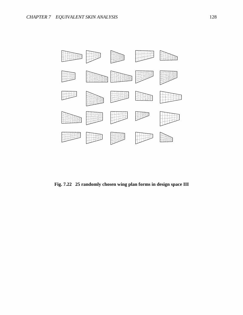
CHAPTER 7 EQUIVALENT SKIN ANALYSIS 128
Fig. 7.22 25 randomly chosen wing plan forms in design space III

CHAPTER 7 EQUIVALENT SKIN ANALYSIS 129
Frequency by EPA
Fre
quen
cyby
ES
A
0 1000 2000 3000 4000 5000 6000 70000
1000
2000
3000
4000
5000
6000
7000
Fig. 7.23 Comparison of the first 10 frequencies by EPA and ESA

CHAPTER 7 EQUIVALENT SKIN ANALYSIS 130
Frequency by EPA
Rel
ativ
eer
ror
0 1000 2000 3000 4000 5000 6000 7000-0.05
0
0.05
0.1
0.15
0.2
Fig. 7.24 The relative errors in Fig. 7.23

CHAPTER 7 EQUIVALENT SKIN ANALYSIS 131
Fig. 7.25 16 wing plan forms systematically varying through design space III
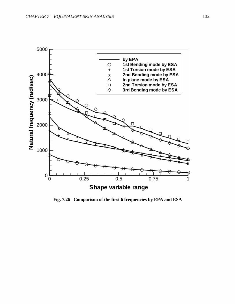
CHAPTER 7 EQUIVALENT SKIN ANALYSIS 132
++
+ + + + + + + + + + + + + +
x
xx
xx
x x xx x x x x x x x
Shape variable range
Nat
ural
frequ
ency
(rad
/sec
)
0 0.25 0.5 0.75 10
1000
2000
3000
4000
5000
by EPA1st Bending mode by ESA1st Torsion mode by ESA2nd Bending mode by ESAIn plane mode by ESA2nd Torsion mode by ESA3rd Bending mode by ESA
+x
Fig. 7.26 Comparison of the first 6 frequencies by EPA and ESA

CHAPTER 7 EQUIVALENT SKIN ANALYSIS 133
Fig. 7.27 An arbitrarily chosen wing plan form in design space III

CHAPTER 7 EQUIVALENT SKIN ANALYSIS 134
Distance from root (inch)
10u,
10v,
w(in
ch)
0 10 20 30 40 50 60 70 80
-3.5E-04
-3.0E-04
-2.5E-04
-2.0E-04
-1.5E-04
-1.0E-04
-5.0E-05
0.0E+00
5.0E-05
10u (EPA)10v (EPA)w (EPA)10u (ESA)10v (ESA)w (ESA)10u (FEM)10v (FEM)w (FEM)
Fig. 7.28 Comparison of displacements by EPA and ESA at 1lb tip force

CHAPTER 7 EQUIVALENT SKIN ANALYSIS 135
Relative distance to leading-edge
Von
Mis
esst
ress
(psi
)
0 0.25 0.5 0.75 10
0.5
1
1.5
2
2.5
3
3.5
Upper skin (EPA)Lower skin (EPA)Upper skin (ESA)Lower skin (ESA)Upper skin (FEM)Lower skin (FEM)
Fig. 7.29 Comparison of the Von Mises stress at wing root by EPA and ESA
under 1lb tip force

CHAPTER 7 EQUIVALENT SKIN ANALYSIS 136
Relative distance to root
Von
Mis
esst
ress
(psi
)
0 0.25 0.5 0.75 11.5
2
2.5
3
3.5
4
Upper skin (EPA)Lower skin (EPA)Upper skin (ESA)Lower skin (ESA)Upper skin (FEM)Lower skin (FEM)
Fig. 7.30 Comparison of the Von Mises stress along central spar by EPA and ESA
under 1lb tip force

CHAPTER 7 EQUIVALENT SKIN ANALYSIS 137
7.2.5 Design space IV
In this case a wing plan with $30=Λ , 192=s in, 72=b in, and 36=a in (see Fig. 6.1 for
definitions of s,b , and a ) is used. A 24 32 × full factorial experimental design with 2 levels in tt0
(skin thickness at wing tip), rta (skin thickness increment ratio at root over the tip), 1h (spar cap
height) and 2h (rib cap height), and 3 levels in sparn and ribn , is carried out. The skins are assumed
to vary linearly from the root to the tip. Particulars of design space III are as follows:
==×=×=
=×=
}.14,10,6{},6,4,2{
,197.0}3,1{,197.0}3,1{
},2,0{,118.0}3,1{
21
0
ribspar
rtt
nn
inhinh
aint
There are 144 sets of data for training. Generating these data sets used much less CPU time
than in the case of design space III. A set of results are given in Figs. 7.31 to 7.33 where 16 points
were randomly chosen within the design space box. The plan forms of the new designs are shown
in Fig. 7.31, where dashed lines indicate the spar or rib positions, and the skin thickness at the wing
root and tip, and cap heights of spars and ribs are represented as shown in Fig. 7.36. The first 10
natural frequencies by the EPA and the ESA are compared in Fig. 7.32 and their relative
differences (based on the EPA results) are shown in Fig. 7.33. It can be seen that the relative
difference is within -5%~15%.
Fig. 7.34 shows 16 new designs through a randomly chosen path inside the design space box
which is defined as
−==
======
=+−=
).1/(,
,,,,,
6,,1,)1(65
24
132
01
10
jjj
nj
ribsparrtt
jjjjj
rrnsa
nnhhvavtv
javavv
j
ννν�
(7.13)
where )6,,1( �=jr j are randomly determined values between 0 and 1, and see Eq. (7.10) for the
definition of other symbols. Results of natural frequencies of the first 6 modes for wing structures
defined by points along the path with n1=0.0031, n2 =0.9999, n3=0.2089, n4 =64.7024, n5 =0.9067

CHAPTER 7 EQUIVALENT SKIN ANALYSIS 138
and n6=0.5325 are shown in Fig. 7.35, where it can be seen that results by the EPA and the ESA
agree with each other quite well.
For an arbitrary new design whose plan form is shown in Fig. 7.36, a down-ward (-z direction)
point force of 1lb is applied at the mid-point of the wing tip. Fig. 7.37 shows displacement
components along the leading-edge by the EPA and the ESA, compared with FEA using
MSC/NASTRAN. Figs. 7.38 and 7.39 show the Von Mises stress distributions at the wing root and
the central spar respectively together with the FEA results. Comparison of the natural frequencies
of this wing as given by the EPA, the ESA and the FEA is shown in Table 7.2. Again, it can be
seen that the EPA and the ESA results are close, and they all agree quite well with the FEA results.
It is noted that a coarser design space III does not worsen the accuracy of the ESA.

CHAPTER 7 EQUIVALENT SKIN ANALYSIS 139
Fig. 7.31 16 randomly chosen wing designs in design space IV

CHAPTER 7 EQUIVALENT SKIN ANALYSIS 140
Frequency by EPA
Fre
quen
cyby
ES
A
0 500 1000 1500 20000
250
500
750
1000
1250
1500
1750
2000
Fig. 7.32 Comparison of the first 10 frequencies by EPA and ESA

CHAPTER 7 EQUIVALENT SKIN ANALYSIS 141
Frequency by EPA
Rel
ativ
eer
ror
0 500 1000 1500 2000
-0.05
0
0.05
0.1
0.15
Fig. 7.33 The relative errors in Fig. 7.32

CHAPTER 7 EQUIVALENT SKIN ANALYSIS 142
Fig. 7.34 16 wing designs systematically varying through design space IV

CHAPTER 7 EQUIVALENT SKIN ANALYSIS 143
+ + + + + + + + + + + + + + + +x x x x x x x x x x x x x x x x
Shape variable range
Nat
ural
frequ
ency
(rad
/sec
)
0 0.25 0.5 0.75 10
100
200
300
400
500
600
700
800
900
1000
1100
1200
1300
1400
1500
by EPA1st Bending mode by ESA2nd Bending mode by ESAIn plane mode by ESA1st Torsion mode by ESA3rd Bending mode by ESA2nd Torsion mode by ESA
+x
Fig. 7.35 Comparison of the first 6 frequencies by EPA and ESA

CHAPTER 7 EQUIVALENT SKIN ANALYSIS 144
Spar cap height (x10)
Rib cap height (x10)
Skin thicknessat root (x10)
Skin thicknessat tip (x10)
Fig. 7.36 An arbitrarily chosen wing design in design space IV

CHAPTER 7 EQUIVALENT SKIN ANALYSIS 145
Distance from root (inch)
10u,
10v,
w(in
ch)
0 50 100 150 200
-7.0E-04
-6.0E-04
-5.0E-04
-4.0E-04
-3.0E-04
-2.0E-04
-1.0E-04
0.0E+00
10u (EPA)10v (EPA)w (EPA)10u (ESA)10v (ESA)w (ESA)10u (FEM)10v (FEM)w (FEM)
Fig. 7.37 Comparison of displacements by EPA and ESA at 1lb tip force

CHAPTER 7 EQUIVALENT SKIN ANALYSIS 146
Relative distance to leading-edge
Von
Mis
esst
ress
(psi
)
0 0.25 0.5 0.75 10
0.1
0.2
0.3
0.4
0.5
0.6
0.7
0.8
0.9
1
Upper skin (EPA)Lower skin (EPA)Upper skin (ESA)Lower skin (ESA)Upper skin (FEM)Lower skin (FEM)
Fig. 7.38 Comparison of the Von Mises stress at wing root by EPA and ESA
under 1lb tip force

CHAPTER 7 EQUIVALENT SKIN ANALYSIS 147
Relative distance to root
Von
Mis
esst
ress
(psi
)
0 0.25 0.5 0.75 10
0.5
1
1.5
2
Upper skin (EPA)Lower skin (EPA)Upper skin (ESA)Lower skin (ESA)Upper skin (FEM)Lower skin (FEM)
Fig. 7.39 Comparison of the Von Mises stress along central spar by EPA and ESA
under 1lb tip force

CHAPTER 7 EQUIVALENT SKIN ANALYSIS 148
7.3 Conclusion
CPU time savings using the ESA are obvious. For instance, when 6 terms of the Legendre
polynomials ( 6=K ) are used, about 85% less CPU time is spent in evaluating the stiffness and
mass matrices compared with the EPA, where matrix evaluating takes about 68% of the total CPU
time when solving the free vibration problem. When 8=K , about 83% less CPU time is spent in
evaluating the matrices compared with the EPA, where matrix evaluating takes about 65% of the
total CPU time. Generally speaking, the results given by the ESA in design space II and III are as
good as those in design space I although the number of variables increases from 4 to 6.
Table 7.1 Natural frequencies (rad/sec) of the wing in Fig. 7.20
Mode No. 1 2 3 4 5Mode Shape 1st bending 2nd bending 1st torsion In plane 2nd torsion
EPA 279.3 982.8 1057.5 1447.4 1945.5ESA 274.5 984.1 1045.1 1440.3 1936.3FEM 279.9 965.6 973.5 1454.4 1830.8
Table 7.2 Natural frequencies (rad/sec) of the wing in Fig. 7.29
Mode No. 1 2 3 4 5Mode Shape 1st bending 2nd bending In plane 1st torsion 3rd bending
EPA 71.9 233.9 358.1 452.2 479.9ESA 70.8 239.4 358.4 469.4 504.8FEM 66.0 222.6 377.0 413.1 468.0

149
Chapter 8
Conclusions and Future Work
8.1 Conclusions of the Present Work
(1) An efficient method capable of static and vibration analyses of the built-up wing structures,
Equivalent Plate-model Analysis (EPA) method, has been developed and comparisons for a
series of examples with commercial FEA calculations have shown the accuracy of the
method for design purposes. On the assumption that the wing structure behaves like a plate
whose deformation can be modeled by the FSDT of Reissner-Mindlin, the Rayleigh-Ritz
method is applied to solve the plate problem, with the Legendre polynomials being used as
the trial functions. The stiffness matrix and mass matrix are determined by applying the
Lagrange’s equations, and can be calculated numerically by using the Gaussian integration
quadrature. Then static analysis can be readily performed and the natural frequencies and
the mode shapes of the wing can be obtained by solving an eigenvalue problem.
Comparison of results by the present method with those by the commercial finite
element analysis code MSC/NASTRAN for a series of 5 vibration problems, 4 static
loading problems, and 1 stress distribution problem showed an overall good agreement
between the two approaches with different methodologies. Mode shapes and natural
frequencies for cases from a thick wing-shaped plate, the same plate with a camber, a solid
wing, to built-up wing structures composed of skins, spars and ribs, have all shown that the

CHAPTER 8 CONCLUSIONS AND FUTURE WORK 150
present method has a fairly good correlation to the FEA, although results for simpler cases
seem to be more accurate. It is also shown that static displacements and stress variation
trends of wing structure can be predicted by the present method quite accurately.
The EPA is formulated mostly in matrix form and calculation can be readily carried out
in the MATLAB environment. It is suitable to be used for the early stages of wing design.
Due to the efficiency of the method, it can also be used as a means to analyze the shape
sensitivity of wing structures.
(2) Modal response of general trapezoidal wing structures was investigated based on an
equivalent model analysis and sensitivity techniques. The variations of the natural
frequencies w.r.t. shape design variables need to be coordinated with the baseline mode
shapes by mode tracking. The use of second order sensitivities proved to be yielding much
better results than the case where only first order sensitivities are used. Shape sensitivities
can be evaluated using analytical, finite difference and semi-analytical approaches. The
present research shows that when the analytical solution is not available, the finite
difference approach would be more accurate than the semi-analytical one provided the step
size is properly specified. But the semi-analytical approach might need less CPU time since
the eigenvalue problem is solved only once.
Neural networks can be trained to relate the natural frequencies of a wing structure to its
shape variables. In this approach the major efforts are in training the networks. Once the
networks are trained, there needs an almost negligible computational effort to obtain
equally good results for the natural frequencies for any given set of the wing shape
variables.
(3) The Equivalent Plate Analysis (EPA) of built-up wing structures is coupled, in an indirect
way, with Neural Networks (NN) to make an even more efficient method, the Equivalent
Skin Analysis (ESA). In the EPA, major part of computational effort is spent on calculating
contributions to the stiffness and mass matrices from each spar and rib. This can be avoided
by replacing the wing inner-structure with an "equivalent" material that combines to the

CHAPTER 8 CONCLUSIONS AND FUTURE WORK 151
skin and whose properties are simulated by neural networks. The constitutive matrix, which
relates the stress vector to the strain vector, and the density of the equivalent material are
obtained by enforcing mass and stiffness matrix equities with regard to the EPA in a least-
square sense. Neural networks for the material properties are trained in terms of the design
variables of the wing structure. Examples show that ESA takes off more than 80% of the
CPU time that is spent in the EPA on computing the total stiffness and mass matrices, and
still fairly good results can be obtained. Therefore, the ESA is very promising to be used at
the early stages of wing structure design.
8.2 Recommendations for Future Work
Generally, the efficient methods developed in the present work (EPA and ESA) can be
extended to deal with all the wing structure problems the FEA can solve, except in cases where
localized solutions are important. Accordingly, these problems can be considered in the early stage
of wing design to shorten design cycle and make better choices. Specifically, developments can be
made at the following area:
(1) To solve complex wings whose planar configuration is composed of 2 or more
quadrilaterals/trapezoids. The extended method should also deal with 3-D cases, that is, the
trapezoidal components can be not in the same plane, as the tail structure considered in
Tizzi 30 . But unlike in Tizzi30 , now all the inner-structure components will be considered.
(2) To extend the present series of efficient methods to deal with steady-state and transient
response problems. Since the stiffness and mass matrices have been given, solution of these
kinds of problems without dissipation should be straightforward. For problems where
structural dissipation is to be considered, work should be done to set up the dissipation
matrix.

CHAPTER 8 CONCLUSIONS AND FUTURE WORK 152
(3) To extend the present series of efficient methods to include geometrical nonlinearity, and
material nonlinearity (plasticity, strain hardening etc.), for problems of large deformation
and in extreme material conditions.
(4) To extend the present series of efficient methods to deal with all spectrum of problems that
are structure-concerned and need to be addressed in wing structure design, such as
aeroelasticity (divergence and flutter speeds), global buckling, and composites/structures
with imperfections or damages.

153
References
1. Gregory Roth, "The Value of Early Analysis", Computer-Aided Engineering, Oct. 1999, pp. 36-
38
2. Housner, J., Draft input to White Paper on Next Generation Revolutionary Analysis and Design
Environment (NEXTGRADE) for Aerospace Systems, Version 3, Feb. 27, 1996
3. Jean Thilmany, "CAD Meets CAE", Mechanical Engineering, Oct. 1999, pp. 66-69
4. Haykin, S., Neural Networks: A Comprehensive Foundation, Macmillan College Publishing
Company, 1994
5. Abdalla, K. M. and Stavroulakis, G. E., "A backpropagation Neural Network Model for Semi-
Rigid Steel Connections", Microcomputers in Civil Engineering, Vol. 10, 1995, pp77-87
6. Vanluchene, R. D. and Sun, R., "Neural Network in Structural Engineering", Microcomputers in
Civil Engineering, Vol. 5, 1990, pp. 207-215
7. Gunaratnam, D. J., and Gero, J. S., "Effect of Representation on the Performance of Neural
Networks in Structural Engineering Applications", Microcomputers in Civil Engineering, Vol. 9,
1994, pp. 97-108
8. Kapania, R. K. and Liu, Y., “Applications of Artificial Neural Networks in Structural
Engineering with Emphasis on Continuum Models”, Technical Report, Virginia Polytechnic
Institute and State University, Blacksburg, VA, June 1998.
9. Liu, Y., Kapania, R. K. and VanLandingham, H., "Simulating and Synthesizing Substructures
Using Neural Network and Genetic Algorithms", Modeling and Simulation Based Engineering, ed.
S. N. Atluri & P. E. O'Donoghue, Tech Science Press, 1998, Vol. I, pp. 576-581

REFERENCES 154
10. Noor, A. K., Anderson, M. S., and Greene, W. H., “Continuum Models for Beam- and Platelike
Lattice Structures”, AIAA Journal, Vol. 16, No. 12, 1978, pp. 1219-1228.
11. Nayfeh, A. M., and Hefzy, M. S., “Continuum Modeling of the Mechanical and Thermal
Behavior of Discrete Large Structures”, AIAA Journal, Vol. 19, No. 6, 1981, pp. 766-773.
12. Sun, C. T., Kim, B. J., and Bogdanoff, J. L., “On the Derivation of Equivalent Simple Models
for Beam- and Plate-Like structures in Dynamic Analysis”, AIAA Paper 81-0624, 1981, pp. 523-
532.
13. Noor, A. K., “Continuum Modeling for Repetitive Lattice Structures”, Applied Mechanics
Review, Vol. 41, No. 7, 1988, pp. 285-296.
14. Lee, U, “Dynamic Continuum Modeling of Beamlike Space Structures Using Finite-Element
Matrices ”, AIAA Journal, Vol. 28, No. 4, 1990, pp. 725-731.
15. Lee, U, “Dynamic Continuum Plate Representations of Large Thin Lattice Structures”, AIAA
Journal, Vol. 31, No. 9, 1993, pp. 1734-1736.
16. Lee, U, “Spectral Element Approach for the Homogeneous Continuum Representations of a
Periodic Lattice Structure”, International Journal of Space Structures, Vol. 12, No. 1, 1997, pp.1-8.
17. Kapania, R. K. and Castel, F., “A Simple Element for Aeroelastic Analysis of Undamaged and
Damaged Wings”, AIAA Journal, Vol. 28, No. 2, 1990, pp. 329-337.
18. Song, O. and Librescu, L., “Free Vibration and Aeroelastic Divergence of Aircraft Wings
Modeled as Composite Thin-Walled Beams”, AIAA Paper 91-1187, 1991.
19. Lee, U, “Equivalent Dynamic Beam-Rod Models of Aircraft Wing Structure”, Aeronautical
Journal, Dec. 1995, pp. 450-457.
20. Lovejoy, A. E. and Kapania, R. K., “Natural Frequencies and Atlas of Mode Shapes for
Generally-Laminated, Thick, Skew, Trapezoidal Plates”, CCMS(Center for Composite Materials
and Structures)-94-09, Virginia Polytechnic Institute and State University, Blacksburg, VA, Aug.
1994.

REFERENCES 155
21. Lovejoy, A. E., “Natural Frequencies and Atlas of Mode Shapes for Generally-Laminated,
Thick, Skew, Trapezoidal Plates”, MS Thesis, Department of Aerospace and Ocean Engineering,
Virginia Polytechnic Institute and State University, Blacksburg, VA, Aug. 1994.
22. Dawe, D. J., “Buckling and Vibration of Plate Structures Including Shear Deformation and
Related Effects”, Aspects of the Analysis of Plate Structures, Ed. by Dawe, D. J., Horsington, R.
W., Kamtekar, A. G. and Little, G. H., New York, Oxford University Press, 1985, pp. 75-99.
23. Reddy, J. N. and Miravete, A., Practical Analysis of Composite Laminates, CRC Press, Inc.,
Boca Raton, 1995, pp. 52-62
24. Reissner, E., “The Effect of Transverse Shear Deformation on the Bending of Elastic Plates”,
Journal of Applied Mechanics, Vol. 12, 1945, pp. A-69~77.
25. Mindlin, R. D., “Influence of Rotatory Inertia and Shear on Flexural Motions of Isotropic,
Elastic Plates”, Journal of Applied Mechanics, Vol. 18, 1951, pp. 31-38.
26. Kapania, R. K. and Raciti, S., “Recent Advances in Analysis of Laminated Beams and Plates,
Part I: Shear Effects and Buckling”, AIAA Journal, Vol. 27, No. 7, 1989, pp. 923-934.
27. Knight, N. F. and Qi, Y., “On a Consistent First-Order Shear-Deformation Theory for
Laminated Plates”, Composites Part B: Engineering, 28 B (1997), pp. 397-405.
28. Giles, G. L., “Equivalent Plate Analysis of Aircraft Wing Box Structures with General
Planform Geometry”, Journal of Aircraft, Vol. 23, No. 11, 1986, pp. 859-864.
29. Giles, G. L., “Equivalent Plate Modeling for Conceptual Design of Aircraft Wing Structures”,
AIAA Paper 95-3945, September 1995.
30. Tizzi, S., “Numerical Procedure for the Dynamic Analysis of Three-Dimensional Aeronautical
Structures”, Journal of Aircraft, Vol. 34, No. 1, 1997, pp. 120-130.
31. Livne, E., “Equivalent Plate Structural Modeling for Wing Shape Optimization Including
Transverse Shear”, AIAA Journal, Vol. 32, No. 6, 1994, pp. 1278-1288.
32. Livne, E. and Navarro, I., “Nonlinear Equivalent Plate Modeling of Wing Box Structures”, 40th
AIAA/ASME/ASCE/AHS/ASC SDM Conference, April 12-15, 1999, St. Louis, MO, pp. 346-372.
Also Journal of Aircraft, Vol. 36, No. 5, 1999, pp. 851-865.

REFERENCES 156
33. Haug, E. J., Choi, K. K. and Komkov, V., Design Sensitivity Analysis of Structural Systems,
Academic Press, Inc., Orlando, Florida, 1986.
34. Adelman, H. M. and Haftka, R. T., "Sensitivity Analysis of Discrete Structural Systems", AIAA
Journal , Vol. 24, No. 5, 1986, pp. 823-832.
35. Barthelemy, J.-F. M. and Haftka, R. T., "Approximation Concepts for Optimum Structural
Design F�D�5HYLHZ���Structural Optimization, Vol. 5, 1993, pp. 129-144.
36. Kapania, R. K., Bergen, F. D. and Barthelemy, J.-F. M., "Shape Sensitivities Analysis of Flutter
Response of a Laminated Wing", AIAA Journal , Vol. 29, No. 4, 1991, pp. 611-612.
37. S. Singhvi, and R. K. Kapania, "Analytical Shape Sensitivities and Approximations of Modal
Response of Generally Laminated Tapered Skew Plates", Journal of Aircraft, Vol. 30, No. 3, 1993,
pp. 423-426.
38. Eldred, L. B., "Sensitivity Analysis of the Static Aeroelastic Response of a Wing", Ph. D.
Dissertation, Virginia Polytechnic Institute and State University, Blacksburg, VA, Feb. 1993
39. Kapania, R. K. and Issac, J. C., "Sensitivity Analysis of Aeroelastic Response of a Wing in
Transonic Flow", AIAA Journal , Vol. 32, No. 2, 1994, pp. 350-356.
40. Bhardwaj, M. and Kapania, R. K., "Shape Sensitivity Analysis of Divergence Dynamic
Pressures", Journal of Aircraft, Vol. 32, No. 4, 1995, pp. 898-901.
41. Issac, J. C. and Kapania, R. K., "Sensitivity of Flutter Response of a Wing to Shape and Modal
Parameters", AIAA Journal , Vol. 33, No. 10, 1995, pp. 1983-1986.
42. Issac, J. C. and Kapania, R. K., "Aeroelastic Analysis of Wings Using Automatic
Differentiation", AIAA Journal , Vol. 35, No. 3, 1997, pp. 519-525.
43. Kapania, R. K. and Singhvi, S., “Free Vibration Analyses of Generally Laminated Tapered
Skew Plates”, Composites Engineering, Vol. 2, No. 3, 1992, pp. 197-212.
44. Singhvi, S., “Analysis, Shape Sensitivities and Approximations of Modal Response of
Generally Laminated Tapered Skew Plates”, Master Thesis, Virginia Polytechnic Institute and
State University, Blacksburg, VA, Sept. 1991.

REFERENCES 157
45. Kapania, R. K. and Lovejoy, A. E., “Free Vibration of Thick Generally Laminated Cantilever
Quadrilateral Plates”, AIAA Paper 95-1350, 1995; AIAA Journal, Vol. 34, No. 7, 1996, 1474-1480.
46. Kapania, R. K. and Lovejoy, A. E., “Free Vibration of Thick Generally Laminated
Quadrilateral Plates with Point Supports”, AIAA Paper 96-1346, 1996; Journal of Aircraft, Vol.
35, No. 6, 1998, pp. 958-965.
47. Cortial, F., “Sensitivity of Aeroelastic Response of Wings Using Equivalent Plate Models”,
Technical Report, Department of Aerospace and Ocean Engineering, Virginia Tech, 1996.
48. R. K. Kapania, Y. Liu, "Wing Vibrations Using FEM & Equivalent Plate Models", 1999 ASME
Mechanics and Materials Conference, June 27-30, 1999, Virginia Tech, Blacksburg, VA 24061
49. Kapania, R. K. and Liu, Y., “Static and Vibration Analyses of General Wing Structures Using
Equivalent Plate Models”, to appear in AIAA Journal. Also, as Paper 2000-1434 at 41st
AIAA/ASME/ASCE/AHS/ASC Structures, Structural Dynamics, and Materials Conference &
Exhibit, 3-6 April 2000, Atlanta, Georgia.
50. Liu, Y. and Kapania, R. K., “Modal Response of Trapezoidal Wing Structures Using Second
Order Shape Sensitivities”, AIAA Journal, Vol. 38, No. 4, April 2000, pp. 732-735.
51. Kapania, R. K. and Liu, Y., “Efficient Simulation of Wing Modal Response: Application of 2nd
Order Shape Sensitivities and Neural Networks”, submitted to 8th AIAA/NASA/USAF/ISSMO
Symposium on Multidiscipline Analysis and Optimization, 6-8 September 2000, Long Beach, CA.
52. Liu, Y. and Kapania, R. K., “Equivalent Skin Analysis of Wing Structures Using Neural
Networks", submitted to AIAA Journal and also to be presented at 8th AIAA/NASA/USAF/ISSMO
Symposium on Multidiscipline Analysis and Optimization, 6-8 September 2000, Long Beach, CA.
53. Hornik, K., Stinchcombe, M. and White, H., "Multilayer Feedforward Networks are Universal
Approximators", Neural Networks, Vol. 2, 1989,pp. 359-366.
54. Hartman, E. J., Keeler, J. D., and Kowaski, J. M., "Layered Neural Networks with Gaussian
Hidden Units as Universal Approximators", Neural Computation, Vol. 2, 1990,pp 210-215.

REFERENCES 158
55. Rabelo, L. C., Shastri, V., Onyejekwe, E. and Vila, J., "Using Neural Networks and Abductive
Modeling for Device-Independent Color Correction", Scientific Computing and Automation, May
1996
56. Ross, C. T. F., Finite Element Methods in Structural Mechanics, Ellis Horwood Ltd., 1985
57. Jang, J.-S. R., Sun, C.-T. and Mizutani, E., Neuro-Fuzzy and Soft Computing: A Computational
Approach to Learning and Machine Intelligence, Prentice Hall, Inc., 1997.
58. Hurty, W. C. and Rubinstein, M. F., Dynamics of Structures, Prentice-Hall, Inc., New Jersey,
1964.
59. Karamcheti, K., Principles of Ideal-fluid Aerodynamics, R. E. Krieger Pub. Co., New York,
1980, pp. 488-490
60. Issac, J. C., “Sensitivity Analysis of Wing Aeroelastic Responses”, Ph. D. Dissertation,
Department of Aerospace and Ocean Engineering, Virginia Polytechnic Institute and State
University, Blacksburg, VA, Nov. 1995.
61. Karpel, M., Moulin, B. and Love, M. H., "Modal-Based Structural Optimization with Static
Aeroelastic and Stress Constraints", Journal of Aircraft, Vol. 34, No. 3, 1997, pp. 433-440.
62. Eldred, M. S., Venkayya, V. B. and Anderson, W. J., "Mode Tracking Issues in Structural
Optimization", AIAA Journal, Vol. 33, No. 10, 1995, pp. 1926-1933.
63. Eldred, M. S., Venkayya, V. B. and Anderson, W. J., "New Mode Tracking Methods in
Aeroelastic Analysis", AIAA Journal, Vol. 33, No. 7, 1995, pp. 1292-1299.
64. Rall, L. B., "Automatic Differentiation: Techniques and Applications", Lecture Notes in
Computer Science, Vol. 120, Springer-Verlag, Berlin, 1981
65. Automatic Differentiation of Algorithms: Theory, Implementation, and Applications, Ed.
Griewank, A. and Corliss, G. F., SIAM, Philadelphia, 1992
66. Wittrick, W. H., "Rates of Change of Eigenvalues, with Reference to Buckling and Vibration
Problems", Journal of the Royal Aeronautical Society, Vol. 66, 1962, pp. 590-591.
67. Fox, R. L. and Kapoor, M. P., "Rates of Change of Eigenvalues and Eigenvectors", AIAA
Journal, Vol. 6, No. 12, 1968, pp. 2426-2429.

REFERENCES 159
68. Friswell, M. I. and Mottershead J. E., Finite Element Model Updating in Structural Dynamics,
Kluwer Academic Publishers, the Netherlands, 1995.
69. Haftka, R. T. and Gurdal, Z., Elements of Structural Optimization, Kluwer Academic
Publishers, the Netherlands, 1992
70. Balabanov, V. O., Giunta, A. A., Golovidov O., Grossman, B., Mason, W. H., Watson, L. T.
and Haftka, R. T., “Reasonable Design Space Approach to Response Surface Approximation”,
Journal of Aircraft, Vol. 36, No.1, January-February 1999
71. Box, M. J. and Draper, N. R., “Factorial Designs, the |X'X| Criterion and Some Related
Matters”, Technometrics, Vol.13, No. 4, 1971, pp. 731-742.
72. Mitchell, T. J., “An Algorithm for the Construction of D-Optimal Experimental Designs”,
Technometrics, Vol.16, No. 2, 1974, pp. 203-210.
73. Nikolaidis, E., Long, L. and Ling, Q., “Neural Networks and Response Surface Polynomials for
Design of Vehicle Joints”, Computers and Structures, 75 (2000), pp. 593-607.
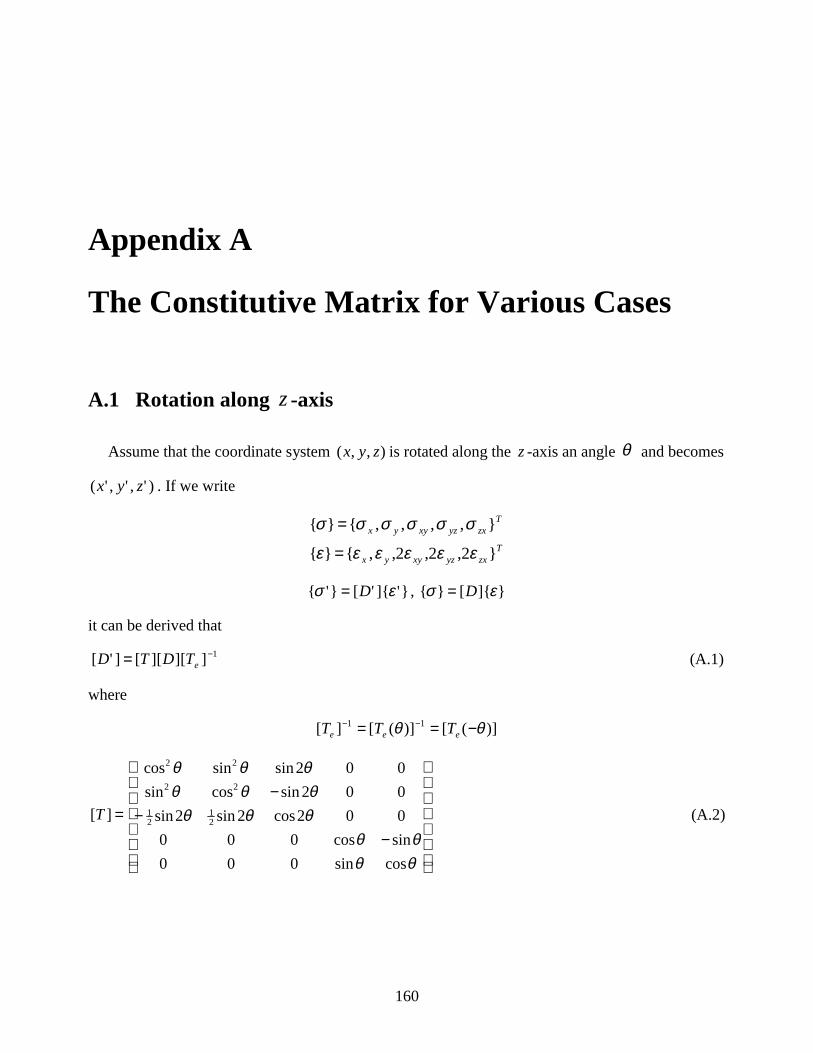
160
Appendix A
The Constitutive Matrix for Various Cases
A.1 Rotation along z-axis
Assume that the coordinate system ),,( zyx is rotated along the z-axis an angle θ and becomes
)',','( zyx . If we write
Tzxyzxyyx
Tzxyzxyyx
}2,2,2,,{}{
},,,,{}{
εεεεεε
σσσσσσ
=
=
}']{'[}'{ εσ D= , }]{[}{ εσ D=
it can be derived that
1]][][[]'[ −= eTDTD (A.1)
where
)]([)]([][ 11 θθ −== −−eee TTT
−−
−=
θθθθ
θθθθθθ
θθθ
cossin000
sincos000
002cos2sin2sin
002sincossin
002sinsincos
][21
21
22
22
T (A.2)

APPENDIX A CONSTITUTIVE MATRIX 161
−−
−=
θθθθ
θθθθθθ
θθθ
cossin000
sincos000
002cos2sin2sin
002sincossin
002sinsincos
][2122
2122
eT (A.3)
A.2 Rotation along y -axis
Assume that the coordinate system ),,( zyx is rotated along the y -axis an angle θ and becomes
)',','( zyx , then the relationship of the constitutive matrices for the two systems can still be
described as in (A.1), but with (A.2) and (A.3) becoming
−
−
=
θθθθθθ
θθθ
2cos0002sin
0cossin00
0sincos00
2sin0010
2sin000cos
][
21
2
T (A.4)
−
−
=
θθθθθθ
θθθ
2cos0002sin
0cossin00
0sincos00
2sin0010
2sin000cos
][21
212
eT (A.5)
A.3 Skin
The local constitutive matrix is

APPENDIX A CONSTITUTIVE MATRIX 162
−−
−−
=
55
44
33
22
22
0000
0000
0000
00011
00011
][
D
D
D
EE
EE
D ννν
νν
ν
(A.6)
where GD =33 , )1(2 ν+
= EG , E is the Young's modulus, ν is the Poisson's ratio, and
kGD =44 , kGD =55 ,6
5=k or 12
2π for thick plates and 044 =D , 055 =D for thin skins.
If the wing has a high aspect ratio and a small swept angle, then we can see ),,( 000 zyx (the
local coordinates) to rotate an angle αθ = (see Fig. 2 for the definition of α )along the y -axis
to coincide with ),,( zyx (the global coordinates), therefore the global constitutive matrix is
1)](][)][([][ −= αα eTDTD
where ][T and ][ eT are found in Eqs. (A.4) and (A.5). If the skin is composed of laminated
layers, for the i -th layer the global constitutive matrix is
1)](][)][([][ −= ieii TDTD θθ
where ][T and ][ eT are found in Eqs. (A.2) and (A.3), and iθ is the orientation angle of the i -
th layer.
A.4 Spar and Rib Cap
Since the cap is slim (i.e. 1/, 11 <<sth ), the spar cap behaves like a 1-D bar. That is, the local
constitutive matrix is
]0000[][ EdiagD = . (A.7)
After a rotation of an angle θ along the z-axis, the global constitutive matrix becomes
1)](][)][([][ −= θθ eTDTD

APPENDIX A CONSTITUTIVE MATRIX 163
where ][T and ][ eT are found in Eqs. (A.2) and (A.3). The angle θ is the angle between the local
orientation of the spar or rib and the x -axis.
A.5 Spar and Rib Web
The local constitutive matrix is
]000[][ GEdiagD = . (A.8)
The global constitutive matrix can be obtained using
1)](][)][([][ −= θθ eTDTD
where ][T and ][ eT are found in Eqs. (A.2) and (A.3), and θ is the angle between the local
orientation of the spar or rib and the x -axis.

164
Appendix B
Formulation for Multi-Plane Problem Using
EPA
As shown in Fig. B.1, a wing is composed of a main-body and a wing-let. What is given in this
appendix can be used as a basis to solve wing structures with more than one wing-let or composed
of more than two planes.
x,
z
y,
1
2
1
2
(ξ ,η )
(ξ ,η )
ξη
Fig. B.1 Sketch for a wing composed of main-body and wing-let

APPENDIX B MULTI-PLANE PROBLEMS USING EPA 165
B.1 Strain Energy and Stiffness Matrix
The total strain energy of the structure:
}]{[}{}]{[}{}]{[}{ 1121
22221
11121 qKqUqKqqKqU BC
TJT
TT +++= (B.1)
where ][ 1K and ][ 2K are the stiffness matrices for the main-body and the wing-let respectively,
whose formulation can be found in Ref. 1, ][ BCK is the stiffness matrix for the large springs
simulating the boundary conditions at the root2 , and JTU is the strain energy relating to the joint
between the main-body and the wing-let, which will be treated as follows.
In the ),( 11 ηξ and ),( 22 ηξ planes, the relationships between the displacement vectors and the
general displacement vectors1 can be written as
==
}]{[}{
}]{[}{
222
111
qHu
qHu (B.2)
where ][ 1H and ][ 2H are functions of ),( 11 ηξ and ),( 22 ηξ respectively. For the joint joining the
main-body and the wing-let, we can have
1,11;1,11 2211 −=≤≤−=≤≤− ηξηξ
and by expressing the displacement vector in plane ),( 22 ηξ in terms of plane ),( 11 ηξ , we get
}]{[}'{ 22 uRu = (B.3)
where }'{ 2u is the displacements of the wing-let expressed in plane ),( 11 ηξ .
Now we can write the strain energy of the joint as
}']{[}'{ 212121 uuKuuU JT
TJT −−= (B.4)
where ][ JTK is the stiffness matrix for the joint, and springs with very large magnitude can be used
if the joint is rigid. Using Eqs. (B.2) and (B.3), Eq. (B.4) can be extended as
( ) ( )( )
( )}]{][][[][][}{
}]{[][][]][[][}{}]{][[][}{
}]{][[][}{}{][][]][[}{}]{[}{
}]{[}{][}]{[}{
222221
221121
111121
2221
2121
1121
212121
qHRKRHq
qHRKRKHqqHKHq
uRKRuuRKRKuuKu
uRuKuRuU
JTTTT
TJT
TJT
TTJT
TT
JTTTT
JTT
JTT
JTT
JTT
JT
+
−−+=
+−−+=
−−=
(B.5)

APPENDIX B MULTI-PLANE PROBLEMS USING EPA 166
A general displacement vector for the whole system can be constructed as
=}{
}{}{
2
1
q
and the total strain energy of the structure can also be written as
( ) }]{[}{}{][][}{}]{[}{
}{
}{
][][
][][
}{
}{}]{[}{
222221
22112121
111121
2
1
2221
1211
2
121
21
qKqqKKqqKq
q
q
KK
KK
q
qqKqU
TTTT
T
T
+++=
== (B.6)
Comparing Eq. (B.6) with Eqs. (B.1) and (B.5), we can obtain the stiffness matrix of the whole
structure
=
][][
][][][
2221
1211
KK
KKK in terms of }{q :
( )
+−==
+=
++=
][][][]][[][][][
]][][[][][][][
][]][[][][][
2121
2112
22222
11111
HRKRKHKK
HRKRHKK
KHKHKK
TJT
TJT
TT
JTTT
BCJTT
(B.7)
B.2 Kinetic Energy and Mass Matrix
The total kinetic energy of the structure:
=+=}{
}{
][0
0][
}{
}{}]{[}{}]{[}{
2
1
2
1
2
121
22221
11121
q
q
M
M
q
qqMqqMqT
T
TT
�
�
�
����� (B.8)
where ][ 1M and ][ 2M are the mass matrices for the main-body and the wing-let respectively1.
Therefore the mass matrix of the whole structure is
=][0
0][][
2
1
M
MM (B.9)

167
Appendix C
Airfoil Sections Generated with the Karman-
Trefftz Transformation
The Karman-Trefftz transformation59 is defined as
n
n
c
c
ncz
ncz
)(
)(
+−=
+−
ςς
(C.1)
where iyxz += is a vector in the −z plane, 1−=i , and ηξς i+= is a vector in the −ς plane.
If 2=n , Eq. (C.1) becomes the Joukowski transformation:
2
2
)(
)(
2
2
c
c
cz
cz
+−=
+−
ςς
or ς
ς2c
z += (C.2)
As shown in Fig. C.1, the Karman-Trefftz transformation in Eq. (C.1) maps a circle in the ς -
plane:
µς θ += iae (C.3)
where )sin(
sin
sin
sin
δβδ
βδ
+⋅=⋅= cma is the radius,
ββδδµ δ sincossincos iaacimmmei +−=+== ,

APPENDIX C KARMAN-TREFFTZ TRANSFORMATION 168
τO
T T'
ξ
η
x
y
(-nc, 0) (nc, 0)
β
δC
C'
(ξ, η) −>(x, y)
The Karman-Trefftz Transformation
)arg()Im(
)Re(tan 1 µς
µηµξθ −=
−−= − ,
to a Karman-Trefftz airfoil section in the z-plane.
More specifically, the transformation in Eq. (C.1) can written as:
ς -plane z-plane
CTaOTcOCmOCCOTOTC ====∠=∠= ,,,,, µδβ
Fig. C.1 The Karman-Trefftz transformation

APPENDIX C KARMAN-TREFFTZ TRANSFORMATION 169
=−=
+==+−
⋅==
+−−⋅==
−
cTAN
crrrr
rnr
nrncyy
rnr
rncxx
nn
n
nn
n
#
#
ξηλλλλ
ηξλληξ
ληξ
12,121
222,121
2
2
2
,
}){(,/
cos21
cos2),(
cos21
1),(
21
(C.4)
in which, a general arc tangent function 1−TAN is defined according to the common arc tangent
function ]2
,2
[tan 1 ππ−∈− :
≥<
+
<<≤≥
+
>≥
=
−
−
−
−
.00,tan2
);00()00(,tan
;00,tan
1
1
1
1
xandyifx
y
xandyorxandyifx
y
xandyifx
y
x
yTAN
π
π (C.5)
If the common arc tangent function 1tan− instead of 1−TAN is used in Eq. (C.4), there would be
some abnormal kinks in the curve in the −z plane transformed from a circle in the −ς plane.
It can be proved that the trailing edge angle of the airfoil is )2( n−= πτ . When ,0,2 == τn so
the Joukowski airfoils have cusped trailing edges.
The camber of the airfoil is determined by βδµ sinsin)Im( am == , and the thickness by
βδµ coscos)Re( acm −== . The chord-length is
−++++=
nn
nn
nclεεεε
)2(
)2(1 (C.6)
where
−= 1cos2 βε
c
a is a quantity of small value having a close relationship with the
thickness. If ,0→ε from Eq. (C.6) we can see that ncl 2→ .
Fig. C.2 shows several airfoils obtained using the Karman-Trefftz transformation with different
combinations of ,, δβ and n.

APPENDIX C KARMAN-TREFFTZ TRANSFORMATION 170
I
II
III
When there is an incoming flow, it is ready to obtain the velocities and pressures at any point,
streamline patterns, and the lift coefficient etc., by using Eq. (C.1) or (C.4) and the velocity
potential of the flow past a circle with circulation.
Fig. C.2 Airfoil shapes obtained using Karman-Trefftz transformation
95.1,85.0,05.0 === nπδβ
9.1,996.0,001.0 === nπδβ
99.1,88.0,05.0 ==−= nπδβ

171
Vita
Youhua Liu was born on August 22, 1963, in Jing County, Hunan Province, China. He attended
the No. 1 Middle School of Jing County for high school education, from September, 1978 to July,
1980, among the first group of students enrolled county-wide since the Cultural Revolution. In
September, 1980, he enrolled at Huazhong (Central China) University of Science and Technology
(HUST), in Wuhan, capital of Hubei Province. Majoring in Naval Architecture and Ocean
Engineering, he earned a Bachelor's degree in engineering in July, 1984. He continued to study and
got a Master's degree in engineering in July, 1987. From 1991 to 1996 he worked at HUST as a
faculty member and research engineer. In 1994, he worked for two months as a visiting scientist at
Yokohama National University, Japan.
In August 1996, Youhua Liu began his study toward a PhD with the Department of Aerospace
and Ocean Engineering, Virginia Tech. Blacksburg is a wonderful place to live in and being a
Hokie is a fantastic experience to him. He is expected to obtain his PhD in aerospace structures in
early 2000.