efficient ray tracing of sparse voxel octrees on an fpga - diva
TRANSCRIPT

Efficient Ray Tracing of Sparse Voxel Octrees on an FPGA
Audun Wilhelmsen
Master of Science in Electronics
Supervisor: Per Gunnar Kjeldsberg, IET
Department of Electronics and Telecommunications
Submission date: June 2012
Norwegian University of Science and Technology


Problem Statement
Ray tracing is a method of generating images of 3D models. It involves tracing light raysin reverse, from a camera to light sources in the scene. Sparse Voxel Octrees (SVO) isa tree-based data structure used to store volumetric pixels. This structure can be usedfor 3D models and can be traversed efficiently, which makes it suitable for ray tracing.Recently there has been efforts to perform ray tracing of SVOs for the purpose of renderingreal-time graphics. There exists pure software implementations and solutions based ongeneral purpose graphics processing units.
Review the existing solution that implement this technique. Outline a design for a systemthat can accelerate this technique in dedicated hardware. Implement a unit that cantraverse SVOs, a control unit which can schedule multiple traversal units and a cache andmemory management that is optimized for the memory access pattern of the traversalunits. Find and implement optimizations that can speed up rendering. Finally, explainhow this system could be integrated with traditional graphics processing units in order torender images using both the proposed technique, and the traditional rendering technique.Discuss the possible challenges that will be encountered.
i

ii

Abstract
Ray tracing of sparse voxel octrees is a method of rendering images of 3D models, whichcould soon become practical for use in real time applications. This is desirable as raytracing can produce very realistic visualizations, while voxel models can represent modelswith very fine geometric detail. For these reason the method has attracted significantattention in recent years, but no hardware solution has been published yet. This thesispresents a design of ray tracing of sparse voxel octrees in hardware. The objective is toshow if it is sensible to implement the method in hardware, and if it could be integrated onmodern GPUs alongside rasterization. To this end, the techniques used in existing soft-ware implementations of this method is reviewed, and an algorithm suitable for hardwareimplementation is presented. The problems of integrating the method with rasterization isexplored, and the algorithm is analyzed and optimized to improve efficiency in hardware.A software implementation is presented, which supports the development of a hardwaredesign. This design is implemented using the Verilog hardware description language, andit has been simulated and synthesized for an FPGA prototype. Multiple versions of thedesign has been synthesized and tested, and to evaluate the impact of design parametersthe test results from these designs is presented. The thesis provides a comprehensive eval-uation of the proposed design, and the results indicate that the algorithm is well suitedfor hardware implementation. Although real-time performance was not achieved, thereare indications that further optimizations should allow real-time performance on the sameplatform, and that a full scale implementation on a modern GPU could probably allowray tracing with a quality which is competitive with rasterization.
iii

iv

Sammendrag
Ray tracing av sparse voxel octrees er en metode for a tegne bilder av 3D modeller, somsnart kan bli praktisk for bruk i sanntidsapplikasjoner. Dette er ønskelig fordi ray trac-ing kan produsere veldig realistiske visualiseringer, mens voxel modeller kan representeremodeller med veldig mye geometriske detaljer. Av disse arsakene har metoden fatt bety-delig oppmerksomhet de siste arene, men ingen hardwareløsning har vært publisert enda.Denne oppgaven presenterer et design for ray tracing av sparse voxel octrees. Hensiktener a vise om det er fornuftig a implementere metoden i hardware, og om den kan integr-eres ved siden av rasterisering pa en GPU. Derfor blir teknikkene som har vært brukt ieksisterende softwareløsninger gjennomgatt, og en algoritme som er passelig for a imple-menteres i hardware presenteres. Problemene med a integrere metoden med rasteriseringhar blitt undersøkt, og algoritmen analyseres og optimaliseres for a forbedre ytelsen ihardware. En software implementering presenteres, som underbygger utviklingen at ethardwaredesign. Dette designet implementeres i hardware spraket Verilog, og har blittsimulert og syntetisert for en FPGA prototype. Flere versjoner av designet har blittsyntentisert og testet, og for a evaluere pavirkningen av designparametere blir disse resul-tatene presentert. Oppgaven gir en omfattende evaluering av det foreslatte designet, ogresultatene indikerer at algoritmen er egnet for implementering i hardware. Selv om san-ntidsytelse ikke ble oppnadd, er det indikasjoner pa at videre optimaliseringen vil kunneføre til sanntidsytelse pa samme platform, og at en fullstending implementering pa enmoderne GPU sannsynligvis vil tillate ray tracing med kvalitet som er konkurransedyktigmed rasterisering.
v

vi

Preface
Computer graphics has always fascinated me, and I have found it highly motivating towork with. A couple of years ago I stumbled over an interview with the co-found andtechnical director of id Software, John Carmack. In it he commented, “there is a verystrong possibility, as we move towards next generation technologies, for a ray tracingarchitecture that [...] involves ray tracing into a sparse voxel octree”. Ray tracing is avery enticing form of rendering, because it closely mimics the nature of light. It can befun to work with because it is easy to get realistic results, but it is hard to make it fast.In April 2010 I e-mailed him asking whether implementing this on an FPGA would bea good idea. To my surprise he replied: “I have actually thought specifically about this– much of the work would be very amenable to an FPGA implementation in a far moreefficient manner than when implemented on general purpose hardware.”. This has servedas a huge source of motivation while working on this thesis.
This project is a testament to the value and maturity of the open source hardware designcommunity. I am confident that open source hardware will become increasingly influentialin the coming years.
I am grateful to everyone who has contributed to the ORPSoC project, which has beenan invaluable platform in this thesis. I am in particular very grateful for the work doneby Stefan Kristiansson who ported ORPSoC to the Atlys prototype board I have beenusing in this thesis. Without it I would surely have spent a lot of time on work that isnot directly relevant to the problems I wanted to explore. It is also amazing the extentof support I received through the members of the ORPSoC IRC chat channel.
Chris McClelland’s “FPGALink” project was also an important tool in simplifying thedevelopment process. It enabled me to write software which could communicate directlywith the FPGA over a USB link. He was also extremely helpful in ironing out issuesrelated to the use of this software. Other tools which have contributed to this thesis are“binvox” by Patrick Min and the “vmath” vector library by Jan Bartipan
My supervisor has been Per Gunnar Kjeldsberg (Department of Electronics and Telecom-munications, NTNU, Trondheim). He has given me some absolutely essential advice onbeing focused and making the right decisions with regards to the scope of the thesis. Moreimportantly, he has given precious encouragement by showing genuine enthusiasm for thevalue of my work.
I would also like to thank my friends in Trondheim who made the time I’ve spent in this
vii

city the best years of my life, and helped me maintain a healthy balance between workand play.
This thesis is dedicated to my grandparents, Arthur and Irene Saunes, who let me staywith them during the last stretch of the thesis. They gave me the perfect environment toconcentrate on my work which gave me some very productive weeks while I was there.
viii

Contents
Problem Statement i
Abstract iii
Sammendrag v
Preface vii
Contents x
1 Introduction 1
2 Background 32.1 Models . . . . . . . . . . . . . . . . . . . . . . . . . . . . . . . . . . . . . . 32.2 Transforms . . . . . . . . . . . . . . . . . . . . . . . . . . . . . . . . . . . 42.3 Perspective Projection . . . . . . . . . . . . . . . . . . . . . . . . . . . . . 52.4 Rasterization . . . . . . . . . . . . . . . . . . . . . . . . . . . . . . . . . . 52.5 Z-buffer . . . . . . . . . . . . . . . . . . . . . . . . . . . . . . . . . . . . . 62.6 Ray tracing . . . . . . . . . . . . . . . . . . . . . . . . . . . . . . . . . . . 62.7 Space Partitioning . . . . . . . . . . . . . . . . . . . . . . . . . . . . . . . 82.8 Sparse Voxel Octree . . . . . . . . . . . . . . . . . . . . . . . . . . . . . . 82.9 Traversal of Voxel Octrees . . . . . . . . . . . . . . . . . . . . . . . . . . . 92.10 Representation of Numbers . . . . . . . . . . . . . . . . . . . . . . . . . . 102.11 Data Cache . . . . . . . . . . . . . . . . . . . . . . . . . . . . . . . . . . . 122.12 FPGA . . . . . . . . . . . . . . . . . . . . . . . . . . . . . . . . . . . . . . 132.13 ORPSoC . . . . . . . . . . . . . . . . . . . . . . . . . . . . . . . . . . . . . 132.14 Digilent Atlys . . . . . . . . . . . . . . . . . . . . . . . . . . . . . . . . . . 14
3 Previous Work 173.1 Software Implementations . . . . . . . . . . . . . . . . . . . . . . . . . . . 173.2 GPU Implementations . . . . . . . . . . . . . . . . . . . . . . . . . . . . . 173.3 Ray Tracing in Hardware . . . . . . . . . . . . . . . . . . . . . . . . . . . 183.4 Data Structures . . . . . . . . . . . . . . . . . . . . . . . . . . . . . . . . . 19
4 An Algorithm for SVO Traversal 214.1 Overview . . . . . . . . . . . . . . . . . . . . . . . . . . . . . . . . . . . . 214.2 Parameters . . . . . . . . . . . . . . . . . . . . . . . . . . . . . . . . . . . 22
ix

CONTENTS
4.3 Child Nodes . . . . . . . . . . . . . . . . . . . . . . . . . . . . . . . . . . . 234.4 Negative Directions and Parallel Rays . . . . . . . . . . . . . . . . . . . . 254.5 The Tracing Kernel . . . . . . . . . . . . . . . . . . . . . . . . . . . . . . . 25
5 A Ray Tracer Geometry Stage 295.1 Normalizing the Octree . . . . . . . . . . . . . . . . . . . . . . . . . . . . 295.2 Generating Primary Rays . . . . . . . . . . . . . . . . . . . . . . . . . . . 305.3 Inverse Perspective Projection . . . . . . . . . . . . . . . . . . . . . . . . . 315.4 Normalizing Ray Length . . . . . . . . . . . . . . . . . . . . . . . . . . . . 315.5 Z-Buffering With Ray Tracing . . . . . . . . . . . . . . . . . . . . . . . . . 31
6 Hardware Optimizations 336.1 Floating Point vs Fixed Point . . . . . . . . . . . . . . . . . . . . . . . . . 336.2 The Decimal Point . . . . . . . . . . . . . . . . . . . . . . . . . . . . . . . 346.3 Stack . . . . . . . . . . . . . . . . . . . . . . . . . . . . . . . . . . . . . . . 346.4 Restarting . . . . . . . . . . . . . . . . . . . . . . . . . . . . . . . . . . . . 366.5 Hardware Optimized Algorithm . . . . . . . . . . . . . . . . . . . . . . . . 37
7 Software Implementation 417.1 SVO Data Structure . . . . . . . . . . . . . . . . . . . . . . . . . . . . . . 427.2 Generating Sparse Voxel Octrees . . . . . . . . . . . . . . . . . . . . . . . 427.3 Software Ray Tracer . . . . . . . . . . . . . . . . . . . . . . . . . . . . . . 437.4 Merging Ray Tracing and Rasterization . . . . . . . . . . . . . . . . . . . 447.5 Cache Profiling . . . . . . . . . . . . . . . . . . . . . . . . . . . . . . . . . 447.6 Results . . . . . . . . . . . . . . . . . . . . . . . . . . . . . . . . . . . . . . 467.7 Discussion . . . . . . . . . . . . . . . . . . . . . . . . . . . . . . . . . . . . 47
8 Hardware Implementation 498.1 Hardware Platform . . . . . . . . . . . . . . . . . . . . . . . . . . . . . . . 498.2 Ray Casting Module . . . . . . . . . . . . . . . . . . . . . . . . . . . . . . 518.3 Scheduler . . . . . . . . . . . . . . . . . . . . . . . . . . . . . . . . . . . . 528.4 Memory Controller . . . . . . . . . . . . . . . . . . . . . . . . . . . . . . . 548.5 Ray Traversal Core . . . . . . . . . . . . . . . . . . . . . . . . . . . . . . . 558.6 Core State Machine . . . . . . . . . . . . . . . . . . . . . . . . . . . . . . 568.7 Testing . . . . . . . . . . . . . . . . . . . . . . . . . . . . . . . . . . . . . 588.8 Results . . . . . . . . . . . . . . . . . . . . . . . . . . . . . . . . . . . . . . 608.9 Discussion . . . . . . . . . . . . . . . . . . . . . . . . . . . . . . . . . . . . 64
9 Conclusions 679.1 Future Work . . . . . . . . . . . . . . . . . . . . . . . . . . . . . . . . . . 68
Bibliography 74
A Attached Files 75
B The Software Ray Tracing Core Functions 76
C The Ray Tracing Core Module 82
x
Chapter 1
Introduction
Ray tracing of sparse voxel octrees (SVO) is a method for rendering images of threedimensional models. It has a wide range of potential applications; medical imaging[31],visualization of scientific data[23], video production[9, 6] and real-time graphics[29, 10, 56].This thesis will outline a practical design for ray tracing of SVOs in hardware.
This method has had some attention in recent years, and there are currently several im-plementations of real-time ray tracing of SVO in software[29, 10, 42, 56]. There are alsoa few implementations of a somewhat similar technique, ray tracing of polygon models,in hardware[43, 64]. Although some algorithms for ray tracing of SVOs seem to be par-ticularly suited for hardware implementation, there seems to have been no such attemptyet.
Making hardware optimized for a specific domain, such as medical imaging, can be pro-hibitively expensive. Technology is often developed and popularized within a consumermarket before being adopted in another domain. Consider the massively parallel gen-eral purpose graphics processor units (GPGPUs). These are now being used to processe.g., scientific and medical data[22], and NVIDIA is producing versions of their GPGPUsspecifically for this market[62, 34]. However, these processors grew out graphics cards forthe consumer gaming industry.
Similarly, this thesis will present a hardware implementation which could conceivably beintegrated in a graphics processing units (GPUs) for consumer games, with the under-standing that this might be the most practical path for developing hardware that canbe used within other domains as well. It should be noted that one can not expect thismethod to supplant the established method of rendering graphics for consumer games:rasterization. There is a large investment in rasterization in terms of toolchains, renderingengines and knowledge. For ray tracing of sparse voxel octrees to gain popularity withingames, it must be implemented alongside rasterization, and it should be possible to use itwithin the same rendering pipeline. This way the method can initially be used for specialeffects, and over time gain more uses as the capabilities of the hardware grows and themind share of the method increases. Consequently, a practical architecture for raytracingof SVOs should be as compatible with rasterization as possible.
1

Chapter 1 Introduction
Using sparse voxel octrees to represent 3D models is a logical evolution of virtual texturingtechniques which have been developed recenty[57, 19, 18]. They can allow full freedom todefine the shape and texture of the models, in addition to being a potentially more efficientway to store the color and geometry data[47]. More importantly, these structures can beray traced efficiently[29, 10]. Although ray tracing is generally slower than rasterization,ray tracing is a much more accurate model of how light behaves, and can enable effectslike accurate reflections, detailed shadows and ambient occlusion[9]. There is also abenefit to developers as expression visual effects with rays of light is more natural andeasy to deal with than the tricks that rasterization employ[48]. As hardware becomesfaster, as demand for more realistic graphics grows, and as algorithms for ray tracingbecome more developed, there may soon come a time when using ray tracing for real-time computer games is feasible. This is effectively demonstrated by Schmittler and Pohlswork of converting existing games to use ray tracing[44].
Field-programmable gate arrays (FPGAs) allow designs for digital integrated circuit hard-ware to be prototyped and tested at a price which is several orders of magnitude cheaperthan making application-specific integrated circuits (ASICs). This thesis uses an FPGAprototype platform with the intention of presenting a design that could later be integratedon an ASIC. Although there are additional challenges to putting a design on an ASIC,an FPGA prototype should solve many of the initial problems.
In this thesis an algorithm for ray tracing of SVOs has been chosen and analyzed. Asoftware implementation has been made to produce reference renderings and behavioralsimulations, which provide data relevant to a hardware implementation. The softwarehas also been used to evaluate techniques to combine rasterization and ray tracing basedrendering. A hardware module which implements the algorithm has been described inthe hardware description language Verilog. This module has been simulated, integratedin a system-on-chip solution for an FPGA, and several variations of the design has beensynthesized, tested and benchmarked. This has provided useful data on the impact ofvarious design parameters.
Chapter 2 presents the background material for the thesis. Topics related to rasterization,ray tracing, sparse voxel octrees, caching techniques and FPGAs are covered. Chapter 3presents previous work which is related to the thesis, and these have been categorized intowork related to software-based ray tracing of SVOs, other forms of ray tracing in hard-ware and work on sparse voxel octree data structures. Chapter 4 presents and explainsan existing algorithm for ray tracing of SVOs, which serves as a good basis for a hardwareimplementation. Chapter 5 discusses some challenges related to integrating ray tracingand rasterization and presents some solutions which should lead to an architecture thatmakes it easier to combine the two techniques. Chapter 6 presents analysis of aspects ofthe algorithm which is significant to a hardware implementation, and modifications to thealgorithm that make it feasible to implement it in hardware. Chapter 7 describes the soft-ware implementation of the hardware optimized algorithm and discusses the results thisproduced. Chapter 8 describes a hardware implementation, the methodology for testingthe resulting design and discusses the results from these tests. Chapter 9 discusses theconclusions drawn from this thesis and future work necesssary to reach a comprehensiveand practical design for ray tracing of SVOs in hardware.
2

Chapter 2
Background
2.1 Models
In 3D computer graphics, we usually want to visualize real world objects. These objectsmust necessarily be represented in the computer by some kind of model. We use a datastructure or a mathematical model to represent these objects. A common way to modelobjects is using polygon models. These are constructed from sheets of polygons. Thepolygons themselves are usually subdvided into triangles, which can be represented bythree points. A normal vector is often also included, which is useful to indicate whichside of the triangle is facing outwards, and how light should behave on it.
Figure 2.1: A triangle based (left) and a voxel based (right) model.
Another way to represent models is through voxels. Voxels are to 3D models what pixelsare to 2D images. You represent the space as a uniform collection of points, and youstore parameters for each of these points. The parameters can be a color value andnormal vector of the voxel. Voxels can be drawn as points, circles or more commonlycubes. Although the cubes result in aliased hard edges, these can be softened throughadaptive blurring techniques[29].
Given a type of model (polygons or voxels), there can be many different ways to renderthat model to a 2D image. Rendering algorithms are usually optimized for one type of
3

Chapter 2 Background
model. Rasterization is optimized for polygon models, and the algorithm presented inthis thesis is optimized for voxel models.
2.2 Transforms
Transforms are essential tools in computer graphics[3]. It takes an entity and moves,rotates, scales or performs any other kind of geometrical conversion. They are usefulfor positioning objects in the scene, moving cameras and lights, etc. The most usefultransforms are linear transforms. These can be represented as a matrix. In computergraphics points, vectors and colors are usually represented as a 4-component vector. Forpoints and vectors these represent the x, y and z-axis, with the fourth component (w)usually being set to 1. The w-component is useful if a transform needs to add a constantto a component. Any combination of linear transforms can then be applied using a 4x4matrix.
Model transform Models are defined within their own coordinate systems. But tomodel a scene with several different models in it, the models must be positioned in acommon coordinate system, the world space. A model of a teapot could be centered inthe origo of its coordinate system, and the nose could point along the z-direction. Themodel transform for the tea-pot could then for instance rotate it around the y-axis to pointat an angle θ and position it at the coordinate (10, 0, 20). The matrix for this example isillustrated below, with p and q being a vector before and after transformation.
M =
cos θ 0 sin θ 0
0 1 0 0− sin θ 0 cos θ 0
0 0 0 1
1 0 0 100 1 0 00 0 1 200 0 0 1
(2.1)
q = Mp (2.2)
View transform The coordinate system of the world space is usually defined in anintuitively useful manner. The ground could for instance be defined to be parallel tothe X-Z plane. A virtual camera could be positioned freely in this space. For renderingalgorithms however, it is useful to have the camera positioned in the origo of the coordinatesystem with the camera looking along the z-axis. The view transform transforms the scenefrom the world space to the camera space (or eye space). The model and view transformcan be combined in a single model-view matrix.
Projection transform A projection transform maps the visible parts of the scene tosome canonical view volume, a simple axis aligned cube with corners at e.g., (−1,−1,−1)and (1, 1, 1). The nearest visible objects are mapped to the near plane (z = −1). Thefurthest visible objects are mapped to the far plane (z = 1). Similarly there is a top,bottom, left and right plane[3]. Anything outside these planes is outside the view of thecamera, and should be ignored.
4

2.3 Perspective Projection
2.3 Perspective Projection
A perspective projection is a projection which closely match how we perceive the world:objects gets smaller as they get further away, and larger when they come closer. Conse-quently in scene space, the far plane is larger than the near plane, while in the canonicalview volume they are equally big. This projection is represented by the following trans-form matrix[3] (for the OpenGL API), where position of the near, far, left, right, bottomand top planes are denoted respectively n, f, l, r, b and t:
Pp =
2nr−l 0 r+l
r−l 0
0 2nt−b
t+bt−b 0
0 0 − f+nf−n − 2fn
f−n0 0 −1 0
(2.3)
After this matrix is applied, the resulting vector must be divided by its w -componentto complete the perspective transform. The w -component has in other words been usedto temporarily store a value which is a linear function of the other components, and allcomponents will be divided by this value. I.e., to get from a view space point q to acanonical view space point v:
v′ = Ppq
v = v′/v′w(2.4)
2.4 Rasterization
The most popular form of 3D rendering today is rasterization of polygon models, or justrasterization for short[59]. It is the technique used by virtually all commercial GPUs.The process of rasterization can be divided into a pipeline. The three conceptual stagesof the pipeline is the application, geometry and rasterizer stages[3]. The application stageis defined by the developer and runs on the CPU, it runs simulations and provides themodels, textures, data and other parameters for the following stages in the pipeline. Thetask of the geometry stage is to apply transforms and effects that work on the geometry ofthe models, and eventually ending up with triangles mapped to a surface that representsthe screen. The triangles are passed on to the rasterizer stage. This stage iterates throughall the given triangles, and generates fragments for every pixel the triangle covers. Thesefragments can be further processed by a pixel shader, a small program that applies per-pixel visual effects. Finally the fragments for each pixel is merged, producing a singlecolor-value for that pixel.
Figure 2.3 illustrates in further detail how the geometry stage works. The model trans-forms positions different models in a common coordinate system. The view transformpositions the camera in the origo, and points it along the z-axis. The perspective trans-form maps the part of the world which is visible to the camera to a canonical view volume.Anything that is outside this volume is discarded. The geometry is then passed on to therasterizer which is responsible for drawing each triangle.
5

Chapter 2 Background
Model & View Transform
Vertex Shading Projection Clipping Screen
Mapping
Geometry stage
Triangle Setup Triangle Traversal Pixel Shading Merging
Rasterizer stage
Application stage
Figure 2.2: A typical GPU pipeline[3]
disc
ard
x
z
x
z
x
z
x
zModel bounding box Camera
Far plane
Near plane
Model Transform View Transform Projection Transform
Image
Figure 2.3: The geometry stage in action
2.5 Z-buffer
When drawing a fragment, it must be possible to determine whether the fragment shouldbe drawn in front of or behind those that were drawn before. This is usually accomplishedusing a Z-buffer (or depth buffer)[3]. When drawing a fragment of a triangle to a pixelin the image, the z-coordinate (in the canonical view volume) of the fragment is storedin the Z-buffer. If the z-coordinate of the fragment is larger than the one in the buffer,we know that the fragment is behind those that were drawn before, and should not bedrawn to the image.
One thing which is important to note about the Z-buffer, is that when using a perspec-tive transform, the value stored in the buffer is not proportional to the distance of thecamera to the fragment. The z-coordinate in the canonical view volume is derived fromEquation 2.4. It can be shown that this implies that the z-coordinate in the canonicalview volume is a function of 1/zc, where zc is the z-coordinate in the camera space.
2.6 Ray tracing
Ray tracing is a method which generates 3D images by tracing the path of a ray of lightin reverse. A virtual camera is defined, with a location and direction. From this camera,rays are traced in to a scene (a collection of objects we want to render). These rays
6
2.6 Ray tracing
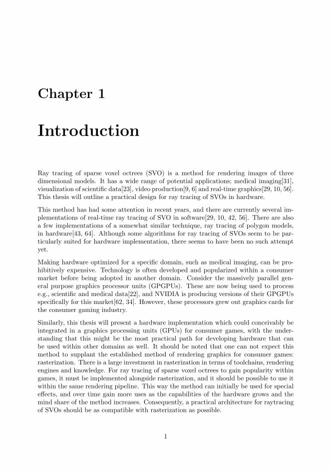
Figure 2.4: An image of the Stanford bunny and a buddha statue, and its Z-buffer. Whiterintensity implies further distance from camera. The background has been colored greento allow the bunny to stand out.
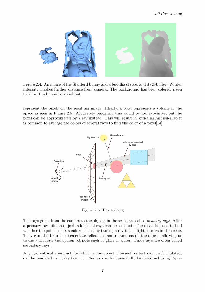
represent the pixels on the resulting image. Ideally, a pixel represents a volume in thespace as seen in Figure 2.5. Accurately rendering this would be too expensive, but thepixel can be approximated by a ray instead. This will result in anti-aliasing issues, so itis common to average the colors of several rays to find the color of a pixel[14].
VirtualCamera
Ray origin
RenderedImage
Pixel
Volume representedby pixel
Primary ray
Light sourceSecondary ray
Figure 2.5: Ray tracing
The rays going from the camera to the objects in the scene are called primary rays. Aftera primary ray hits an object, additional rays can be sent out. These can be used to findwhether the point is in a shadow or not, by tracing a ray to the light sources in the scene.They can also be used to calculate reflections and refractions on the object, allowing usto draw accurate transparent objects such as glass or water. These rays are often calledsecondary rays.
Any geometrical construct for which a ray-object intersection test can be formulated,can be rendered using ray tracing. The ray can fundamentally be described using Equa-
7
Chapter 2 Background
tion 2.5. The ray has an origin o and a direction vector d. t can be considered a virtualtime parameter, and p a position along the ray at different times. In these terms raytracing is the problem of finding the values t where the ray intersect objects.
p(t) = o + t · d (2.5)
This equation can for instance be solved for the equation of a perfect sphere, which iscommonly used to demonstrate simple ray tracers. Equation 2.5 can also be solved fora triangle[14], making it possible to ray trace polygon models. A naive implementationof this would do an intersection test on every triangle in the model for every pixel in thescreen, making the algorithm very slow. To optimize ray tracing, a space partitioningdata structure is often used. Instead of testing every primitive, one performs a searchof this data structure instead to find a set of primitives the ray could intersect. There-fore, ray tracing is cited as having the advantage over rasterization in that performancedepends logarithmically, not linearly, on geometric complexity[25]. Although it shouldbe mentioned that level-of-detail (LOD) based techniques to achieve similar performancescaling exists for rasterization[20].
2.7 Space Partitioning
Space partitioning is a method where a given space is divided into smaller non-overlappingspaces. These sub-spaces can be arranged in a hierarchical tree, where each sub-space canbe divided into further partitions. This results in a nonuniform spatial subdivision[14].Space partitioning data structures is often used in computer games to accelerate certainoperations. In rasterization, it can used to exclude regions of polygons that will not berendered (occlusing culling[7]), or to sort objects by depth, which is important for certainvisual effects[3]. For these purposes, the BSP/kd-tree structures have been found to bebetter than octrees[55]. Although kd-trees have been used for ray tracing voxel data[52],sparse voxel octrees seem particularly suited for this purpose because they can be tracedby a remarkably simple algorithm which will be presented in a later chapter.
2.8 Sparse Voxel Octree
An octree is a hierarchical space-partitioning data structure[41] where a space is dividedin eight equal sub-regions, or octants, and where each octant that contains objects isfurther divided until the resulting tree reaches a desired height. A voxel is a volumetricpixel, in other words, an axis-aligned rectangular prism[14]. A sparse voxel octree is adata structure used to store a voxel model when most of the voxels are empty (the spaceis “sparse”). In visualization of real-world objects, this would be the case, as all the voxelsexists on the surface of objects.
Often, when using a space-partitioning data structure, a list of objects is stored in theleaf nodes. In a sparse voxel octree the leaf node is a voxel, either an empty space or asolid cube. A solid voxel may have a color value. For an inner node, we can take the
8

2.9 Traversal of Voxel Octrees
32
76
10
54
Root
32
76
10
54
Figure 2.6: An octree with 2 levels and a single solid voxel
average color of all the child nodes, and attach it to this node. Doing so means the scenerepresented by the tree can be rendered at varying resolutions, depending on how deep wetraverse. This is desirable because it is a waste to render objects that are far away withhigh detail. Furthermore, we can even avoid loading into memory those parts of the treethat represent high detail in far away parts of the scene, and stream them into memoryas the camera moves towards those areas[10].
2.9 Traversal of Voxel Octrees
A variety of algorithms to traverse space partitions have been described in the literature.They have different complexities, and they can have very different performance on a givencomputer architecture. A significant attribute of the algorithms are whether they use astack or not. A stack is useful for keeping track of the path taken as the tree is traversed,but can be detrimental on certain architectures. The following are descriptions of a fewof the most common methods.
Restart The simplest methods are those based on the kd-restart algorithm. This is astack-less algorithm: A starting point, the ray origin, is chosen. The tree is traverseduntil the voxel representing this point is found. If the voxel represented by the node isempty, the point is moved to where the ray exits the voxel. The algorithm then restartsfrom the new point. In other words, the algorithm traverses one octant at a time, andhas to descend the tree from the root node down every iteration. This is repeated untila collision is found, or the ray exits the voxel represented by the root node.
Backtrack Backtracking algorithms (or push-down optimization [21]) are similar to kd-restart. But it exploits the fact that we can keep track of the last node which must beparent to all the nodes traversed by the ray. It is a simple optimization than can providea performance boost. But the parent node might be close to the root, which can makethe gain minimal in some iterations. It only eliminates traversal steps near the top of thetree, which are the ones that are most shared by neighboring primary rays [21].
9

Chapter 2 Background
Full stack A tree traversal algorithm can use a stack to keep track of the nodes visitedas the algorithm descends the tree. The algorithms utilizing a stack is similar to therestarting algorithms when descending the tree, but will push the traversal state to astack for each node. If an empty space is found, the stack is unwounded until it finds thenext node the ray intersects. The descent can continue as usual from that point. In thisthesis the algorithms using a stack as deep as the tree the algorithm was designed for isreferred to as full stack algorithms, to distinguish them from short stack algorithms.
Short stack Sometimes a full stack can be too expensive to implement. In GPGPUimplementations, the processing cores are often not optimized for the memory accesspattern required by the stack. An alternative is to keep the state for the last Ns nodestraversed. If the stack is exhausted (a stack underflow), the algorithm can perform arestart.
The restarting algorithms can be considered a special case of a short stack with Ns = 0.Similarly, a full stack can be considered a special case with Ns = Nt where Nt is thedepth of the octree. Even if an algorithm is designed with a full stack, it could be wiseto support restarts, as it will allow the algorithm to support octrees deeper than it wasoriginally designed for.
Bottom up methods Revelles et al. [41] describes bottom-up methods as those start-ing at the first terminal node intersected by the ray. The algorithm must then findthe neighboring nodes by some method. Some algorithms use neighbor pointers in theoctree[15], which are pointers stored in the leaf nodes, pointing to the neighboring nodesat each face of its voxel. This enables the algorithm to jump between nodes withoutascending the tree. It can improve traversal speed, but at a significant memory cost, asthe additional pointers have to be stored in the octree.
2.10 Representation of Numbers
There are several ways to represent numbers. For performing calculations, the two mostpopular schemes are probably fixed point and floating point representations. They bothhave strength and weaknesses.
Fixed point numbers The fixed point format is named so because the decimal point isfixed in one place. Equation 2.6 shows the number 5.625 represented in binary fixed-point,with three bits for the integer and fractional part, or a total of six bits.
101.101
1 · 22 + 0 · 21 + 1 · 20 + 1 · 2−1 + 0 · 2−2 + 1 · 2−3(2.6)
The position of the decimal point must be chosen carefully. It will determine what rangeof numbers can be represented, and how accurately they can be represented. Given N
10

2.10 Representation of Numbers
number of integer bits, and a two’s complement representation, the range of integers is−2N−1 to 2N−1 − 1. Given M number of fractional bits, the smallest fraction that canbe represented is 2−M .
Fixed point numbers are relatively cheap to implement in hardware. Table 2.1 shows theresource use of a 32 bit adder/subtract unit and a 32 bit multiplier unit, as estimated bythe Xilinx Core Generator tool[67, 65].
FPGA Operation LUTs FF Latency DSPs Max Clock Freq.
Virtex-5 Add/Subtract 70 91 3 0 410MhzVirtex-5 Add/Subtract 32 32 0 0 388MhzSpartan-6 Multiplier(35x35) 58 107 8 4 250Mhz
Table 2.1: Resource use of fixed point operations[67, 65]
Floating point numbers Floating point numbers are similar to scientific notation;it represents numbers of the form m · 2e−b. A standard for floating point representationcalled IEEE 754[1] is now used almost exclusively in digital computing platforms[24]. Thenumbers are stored as a mantissa, m, and an exponent, e. The exponent is offset by a con-stant bias, b. A sign bit, S, indicates whether the number is positive or negative. Floatingpoint numbers provide a much larger dynamic range than fixed point numbers given thesame amount of bits. That is, it is possible to represent both very large and very smallnumbers in the same representational system. This has several benefits over fixed pointnumbers, one being that the programmer or hardware designer does not have to worry asmuch about overflowing the boundaries of the representation. Floating point numbers areessential in modern GPUs, and a modern high-end GPU can perform over 1000 billionfloating point operations per second[60]. Table 2.2 shows the estimated resource use forsingle precision (32 bit) floating point numbers[66]. Comparing to Table 2.1, we see thatfloating point numbers are significantly more expensive to implement.
31 30 23 22 0S Exponent Mantissa
Figure 2.7: Bit organization of single precision (32 bit) IEEE 754 floating pointrepresentation[1].
FPGA Operation LUTs FF Latency DSPs Max Clock Freq.
Virtex-5 Add/Subtract 432 558 12 0 420MhzVirtex-5 Add/Subtract 388 76 2 0 110MhzSpartan-6 Multiplier 140 187 8 0 150Mhz
Table 2.2: Resource use of floating point operations[66]
11

Chapter 2 Background
2.11 Data Cache
Processors can perform operations on its internal registers significantly faster than it canaccess its main memory. For modern systems the cost of accessing main memory can beabout 120 times as much as accessing a register [39]. It has long been known that using acache can improve the practical cost of accessing main memory. A cache is a fast memorywhich can hold some of the content of the main memory, and which is inserted betweenthe processor and main memory, sometimes with multiple levels of increasingly faster andsmaller caches.
Registers
Level 1 Cache
Level 2 Cache
Main Memory
Bigger mem
ory size
Faster access time
Figure 2.8: A cache hierarchy
A cache exploits two features inherent in the way many algorithms access memory: tem-poral locality and spatial locality. Temporal locality refers to cases where the algorithmaccesses the the same content several times in a small amount of time. Spatial locality iswhere the algorithm accesses memory that is located nearby the last address it accessed.When the processor attempts to access main memory, the cache will be checked to seeif it contains the relevant word. If it did (a cache hit) the cache will return the data. Ifit did not (a cache miss) the cache will fetch the data from main memory, usually in ablock (or “line”) of several words at a time. The ratio of cache misses over the number ofaccesses is called the miss rate, and can be used as a simple indicator of the performanceof the cache [17].
The cache can be considered to have a set of slots in which the blocks can be inserted.Each slot will have an associated tag which indicates the address of the block which isstored there. There are different ways of determining the position of a block in the cache[39]:
Direct mapped : Each block is mapped to a single slot. This implies that when a newblock is fetched, the old block occupying its slot must be evicted.
N-way set associative : Each block is mapped to one of N slots. When fetching anew block a replacement policy determines which of the old slots are chosen. A commonpolicy is least recently used (LRU). The policy tracks the usage of blocks and the blockthat was used least recently will be evicted in favor of the new one.
12

2.12 FPGA
Fully associative : A block can be inserted into any slot. This implies that we mustcompare the tags of all the slots in the cache to determine if a word is present or not.
These approaches have various pros and cons. A direct mapped cache is cheap to im-plement, but will have a lower hit rate. An N-way set associative cache requires morelogic, and higher N implies a higher cost. The cost is also dependent on the replacementpolicy. LRU is cheap to implement in a 2-way set associative cache, requiring only asingle bit to track which block was used last. For 4 and 8-way set associative cache, usinga LRU policy can become prohibitively expensive and some implementations opt for apseudo-LRU policy [53, 13].
2.12 FPGA
A field-programmable gate array (FPGA) is a type of integrated circuit which can beprogrammed (or configured) to perform the function of almost any kind of digital circuitor system[28]. The FPGAs is an array of logic blocks, memory and a routing fabric whichconnects these together. The logic blocks, or look-up tables (LUTs), can be configuredto perform arbitrary combinatorial functions on a number of inputs. FPGAs can alsocontain some specialized blocks. The FPGA used in this thesis contains for example digitalsignal processing and memory controller blocks[68]. These specialized blocks implementcommonly used functions and using these is more efficient than implementing the samefunctions in the general logic blocks.
Although FPGAs are use more area, consume more power and are slower than application-specific integrated circuits (ASICs), they are still very useful due to significantly smallerinvestment costs in terms of both time and money[28]. It is therefore beneficial for projectswith low volume productions or short development time, or for prototyping and testing.
2.13 ORPSoC
OpenRISC Reference Platform SoC (“ORPSoC”) is a project aimed at creating an open-source platform for OpenRISC development. The current version of ORPSoC uses theOpenRISC processor OR1200 and integrates it in a system with several other modules andinterfaces. The system includes modules for JTAG, Ethernet MAC, on-chip RAM/ROM,SPI, UART, I2C and USB. Every module in the system is connected through the Wish-bone bus. There are derivate configurations available for a few different FPGA boards,both based on Actel and on Xilinx.
Wishbone[35] is an open-source hardware bus standard, and specifies the interface betweencomponents in an ASIC or FPGA design. It is an effort by the OpenCores communityto develop a common interface between open-source hardware components, and it’s usedby many of the modules available on the OpenCores website. The standard only specifiesthe digital signals and their protocol. Analog effects or bus topology is intentionally leftambiguous.
Data is transferred during an interval called a bus cycle. During a bus cycle the master will
13

Chapter 2 Background
request a read or write operation on a slave and the relevant data will be transferred. Ofparticular interest in this thesis is burst cycles, which is an optional feature of Wishbone.In a 32-bit Wishbone bus, a single 32-bit word is the most that can be transferred in asingle clock cycle. By using burst cycles the master can negotiate the transfer of multipleconsecutive words during a single bus cycle. This provides two benefits: it avoids havingto set up a new bus cycle for each word and it allows the slave to know up front thenext address that should be transferred. This can potentially allow it to service thefollowing requests with less delay. When negotiating a burst cycle, the master providesthe first address that should be transferred and indicates how the next addresses shouldbe calculated. There are four ways the addresses can be incremented: linear, wrap-4,wrap-8 and wrap-16. With the linear mode the address is incremented linearly for eachtransfer, while with wrap-4, wrap-8 and wrap-16, the address is looped around a 4, 8 or16 word block boundary. This feature is useful for reading cache lines for the cache of aprocessor. The word that the processor requested can be fetched first and sent directly tothe processor, allowing it to continue executing, while the rest of the words in the cacheline can be transferred subsequently.
Wishbone B4
Some signals may or may not be present on a specific interface. That’s because many of the signals are optional.
Two symbols are also presented in relation to the [CLK_I] signal. These include the positive going clock edge transition point and the clock edge number. In most diagrams a vertical guideline is shown at the positive-going edge of each [CLK_I] transition. This represents the theoretical transition point at which flip-flops register their input value, and transfer it to their output. The exact level of this transition point varies depending upon the technology used in the target device. The clock edge number is included as a convenience so that specific points in the timing diagram may be referenced in the text. The clock edge number in one timing diagram is not related to the clock edge number in another diagram.
Gaps in the timing waveforms may be shown. These indicate either: (a) a wait state or (b) a portion of the waveform that is not of interest in the context of the diagram. When the gap indicates a wait state, the symbols ‘-WSM-‘ or ‘-WSS-‘ are placed in the gap along the [CLK_I] waveform. These correspond to wait states inserted by the MASTER or SLAVE interfaces respectively. They also indicate that the signals (with the exception of clock transitions and hatched regions) will remain in a steady state during that time.
Undefined signal levels are indicated by a hatched region. This region indicates that the signal level is undefined, and may take any state. It also indicates that the current state is undefined, and should not be relied upon. When signal arrays are used, stable and predictable signal levels are indicated with the word ‘VALID’.
1.5 Signal Naming Conventions
All signal names used in this specification have the ‘_I’ or ‘_O’ characters attached to them. These indicate if the signals are an input (to the core) or an output (from the core). For example, [ACK_I] is an input and [ACK_O] is an output. This convention is used to clearly identify the direction of each signal.
Signal arrays are identified by a name followed by a set of parenthesis. For example,
Back to TOC Copyright © 2010 OpenCores Page 14 / 128
Illustration 1-2: Standard connection for timing diagrams.
C L K _ I
A D R _ O ( )
D A T _ I ( )
D A T _ O ( )
W E _ O
S E L _ O ( )
S T B _ O
A C K _ I
C L K _ I
A D R _ I ( )
D A T _ I ( )
D A T _ O ( )
W E _ I
S E L _ I ( )
S T B _ I
A C K _ O
WISH
BONE
MAS
TER
WISH
BONE
SLA
VE
C Y C _ O C Y C _ I
T A G N _ O T A G N _ I
R S T _ I R S T _ I
T A G N _ I T A G N _ OU S E R
D E F I N E D
S Y S C O N
Figure 2.9: Wishbone signal lines[35]
OpenRISC is an effort to develop a series of general purpose, open-source RISC CPUdesigns. There is currently one OpenRISC architecture, called OpenRISC 1000. The firstimplementation is OpenRISC 1200 (“OR1200”). The OR1200 is a 32-bit scalar RISCwith Harvard micro-architecture (separate data and instruction interface), 5 stage integerpipeline, IEEE 754 compliant single precision FPU, virtual memory support (MMU) andbasic DSP capabilities[36]. It includes an 8KB data cache and an 8KB instruction cacheby default. The data and instruction interfaces is implemented as a Wishbone interface.
2.14 Digilent Atlys
Atlys is an FPGA prototype board made by Digilent. It uses a Spartan-6 XC6SLX45FPGA chip. The FPGA chip has 43,661 logic cells (27,288 6-input LUTs), 54,576 flip-
14

2.14 Digilent Atlys
flops and 116 18Kbit Block RAM blocks (total 2,088Kbit)[68]. The Atlys prototype boardincludes 128Mbyte DDR2 RAM, an Ethernet port, two HDMI inputs, two HDMI outputs,an AC-97 codec, a 16Mbyte SPI Flash, USB Keyboard/Mouse input, 8 LEDs, 8 switches,5 push buttons, a 100MHz clock and two expansion ports[11]. The FPGA is programmedthrough a Cypress CY7C68013A-56 USB microcontroller. This microcontroller is hascommunication lines connected to the FPGA which can be used to communicate with theconfigured FPGA from a personal computer.
15

Chapter 2 Background
16

Chapter 3
Previous Work
No hardware implementations of ray tracing of SVOs was found in the literature. Thework this project builds on can be divided in four categories: implementations of raytracing of SVOs in software, implementations in GPUs, implementations of other formsof ray tracing in hardware and work related to data structures for SVOs.
3.1 Software Implementations
These works are all in software on CPUs, which is typical for papers from the 90s, asGPGPUs were not available yet. The first descriptions found of octree traversal was as avolume rendering technique by Levoy [31]. It illustrates that introducing the hierarchicaloctree structure improves voxel traversal speed. The next works are the SMART algo-rithm by Spackman and Willis [49] and an algorithm by Stolte and Caubet [51]. They areboth based on a 3D DDA (Digital Differential Analyzer) as described by Sung [54], whichworks by stepping through the space by adding a delta value to a vector. Revelles et al.[41] presents an algorithm based on keeping track ray parameters (t from Equation 2.5)for the voxels during traversal. It appears to be the first work that constructs an algo-rithm which is specifically optimized for traversing octrees. The algorithm is comparedto three previous bottom-up algorithms, and one top-down algorithm, and it was foundto have improved performance over existing algorithms. A paper by Whang et al. [58]was also reviewed. It presents a variation of octrees where the middle planes could beshifted. This made it possible to balance the tree depending on the content of the scene.However, it was not intended for rendering voxels, as the resulting voxels would not beequilateral.
3.2 GPU Implementations
The arrival of GPGPUs allowed new rendering techniques to be implemented. Gobbettiet al. [15] implemented one of the first techniques for ray casting octrees on the GPU.
17

Chapter 3 Previous Work
Their algorithm is based on an extension of an efficient ray traversal algorithm for kd-trees. Crassin et al. [10] presents a full ray tracing architecture for GPUs, which is capableof streaming parts of the octree to the GPU on demand. Their work is similar to thatof Gobbetti et al. [15], but provides better quality and performance. Their algorithm isbased on kd-restart, and avoids the use of a stack which is potentially inefficient on aGPU. The solution is geared towards rendering large volumetric data sets, e.g., medical3D images.
Laine and Karras [29] created an implementation that utilizes a stack, and the algorithmappears nearly identical to that of Revelles et al. [41]. It is not clear why they chose to usea stack, but considering it was research by NVIDIA, who makes GPGPUs, it is probablyan informed choice. Another difference from Crassin et al. [10] is that the implementationis made more suitable for rendering surfaces than volumetric data, which they claim ismore relevant for most real-world content.
A master thesis by Romisch [42] presented three implementations: one using a bottom-upmethod utilizing neighbor pointers, the second using a kd-restart based method, and thethird using a short stack. Neighbor pointers was found to be fastest, but at the costof some flexibility. Between kd-restart and short stack, kd-restart was fastest. It’s hy-pothesized that it’s because of the limited performance of GPU processors when complexcontrol-flow statements are used.
Romisch [42] and Laine and Karras [29] both explored short stacks on GPGPUs butcame to differing conclusions. Romisch and Møller-Nielsen found that using a stack, evena short one, resulted in worse performance. While Laine found that a full stack wasbetter than a short stack. This could possibly be due to different GPGPU architectures,or that the specifics of the implementations are different. In a hardware implementation,this issue is also particularly interesting, as the stack will require registers that consumearea. This area could be used for other logic that could improve performance. Anotherimportant consideration is memory bandwidth. A short stack or restart algorithm willrequire more node lookups, causing more traffic on the data bus.
3.3 Ray Tracing in Hardware
The only hardware designed for ray tracing found in the literature are two prototypes byWoop and Schmittler from the computer graphics laboratory at Saarland University[43,64]. They render polygon data, and use a kd-tree as an space partition structure toaccelerate ray tracing. The first prototype is a fixed function ray tracer called SaarCOR.The second is a programmable ray processing unit (RPU), which allows for higher qualityin the rendered image at the cost of area or performance. Presumably the kd-tree traversalunit described in these papers bears some similarity to the octree traversal unit in thisthesis. Unfortunately the papers do not go into detail regarding the traversal unit, exceptto mention that it uses a stack and requires 4 adders, 4 dividers, 13 comparators and44.5KB of internal memory.
18

3.4 Data Structures
3.4 Data Structures
There are many ways to encode an octree. The main considerations is to compress thesize of the encoded octree as much as possible without making decoding of the structuretoo expensive. A naive implementation would have 8 child pointers for each inner node,which would either point to another innor node, or leaf data. One optimization to thisscheme is to store data about child nodes within the inner nodes as a set of flags[6, 29].Each node can be either an empty octant, an inner node, or a solid voxel. Using 2 bitsto represent these three states for each child results in 16 bits of data. Instead of havinga pointer to each child node, a single pointer can point to an array of node data. Thesize of this pointer depends on the potential size of the octree file. Laine and Karras [29]showed that if we use a relative pointer and organize the data in a depth-first order, 15bits is enough for most child pointers. For the few cases where the pointer falls outsidethe 15-bit range, an additional bit indicates that the pointer is a far pointer, which pointsto a 32-bit pointer instead. The contour pointer and page header/info section shown inFigure 3.1 is used to refine the shape of the voxels and attach additional data to them.
Octree-based geometry compression is introduced by Botsch et al. [8] and Peng et al. [38].Schnabel and Klein [45] builds on this work and presents a method for compression ofpoint-sampled models. The general idea is that it is possible to predict the configurationof a child node as you descend the tree, and that this can be exploited by storing thisconfiguration using variable-length encoding. These techniques obviously add complexityto the encoding and decoding of the octree, but the size of the encoded octree is smaller.
2 Previous Work
There is a vast body of literature on visualizing volumetric struc-tures, so we will focus on papers that are most directly related toour work. We specifically omit methods that are restricted to heightfields (see e.g. [Dick et al. 2009] for a recent contribution) or arebased on a combination of rasterization and per-pixel ray castingin shaders (see [Szirmay-Kalos and Umenhoffer 2008] for an ex-cellent survey) because these are not capable of performing genericray casts.
Amanatides and Woo [1987] were the first to present the regulargrid traversal algorithm that is the basis of most derivative work,including ours. The idea is to compute the t values of the nextsubdivision planes along each axis and choose the smallest one inevery iteration to determine the direction for the next step.
Knoll et al. [2006] present an algorithm for ray tracing octrees con-taining volumetric data that needs to be visualized using differentisosurface levels. Their method is conceptually similar to kd-treetraversal, and it proceeds in a hierarchical fashion by first deter-mining the order of the child nodes and then processing them re-cursively. The algorithm is not as such well suited for GPU im-plementation. An extension to coherent ray bundles is given byKnoll et al. [2009].
Crassin et al. [2009] present a GPU-based voxel rendering algo-rithm that combines two traversal methods. The first stage castsrays against a regular octree using kd-restart algorithm to avoid theneed for a stack. The leaves of this octree are bricks, i.e. 3D grids,that contain the actual voxel data. When a brick is found, its con-tents are sampled along the ray. Bricks typically contain 163 or 323
voxels, yielding a lot of wasted memory except for truly volumetricdata. On the other hand, mipmapped 3D texture lookups supportedby hardware make the brick sampling very efficient, and the result isautomatically antialiased. An interesting feature of the algorithm isthe data management between CPU and GPU. The renderer detectswhen data is missing in GPU memory and signals this to the CPU,which then streams the needed data in. This way, only a subset ofnodes and bricks needs to reside in GPU memory at any time.
Ju et al. [2002] augment an octree structure with auxiliary data toimprove fine geometric details. While the Hermite data utilized bytheir representation is flexible in its ability to support dynamic CSGoperations, a separate triangulation pass is required to render theresulting surface. Our contour-based representation, on the otherhand, aims for efficient rendering and compact storage given theassumption of static geometry.
3 Voxel Data Structure
We store voxel data in GPU memory using a sparse octree datastructure where each node represents a voxel, i.e. an axis alignedcube that is intersected by surface geometry. Voxels may be furthersubdivided into smaller ones, in which case both the parent voxeland its children are included in the octree. The data structure hasbeen designed to minimize the memory footprint while supportingefficient ray casts. Sometimes both can be achieved at the sametime, because more compact data layout also reduces the memorybandwidth requirements.
To this end, we adopt a scheme where most of the data associatedwith a voxel is stored in conjunction with its parent. This removesthe need to allocate storage for individual leaf voxels and makescompression of shading attributes more convenient.
On the highest level, our octree data is divided into blocks. Blocksare contiguous areas of memory that store the octree topology alongwith voxel geometry and shading attributes for localized portions
Figure 2: 64-bit child descriptor stored for each non-leaf voxel.
Figure 3: Layout of the child descriptor array. Left: Example voxelhierarchy. Right: Child descriptor array containing one descriptorfor each non-leaf voxel in the example hierarchy.
of the octree. All memory references within a block are relative,making it easy to reorganize blocks in memory. This facilitatesdynamic memory management necessary for out-of-core rendering.
Each block consists of an array of child descriptors, an info section,contour data, and a variable number of attachments. The child de-scriptors (Section 3.1) and contour data (Section 3.2) encode thetopology of the octree and the geometrical shape of voxels, re-spectively. Attachments (Section 3.5) are separate arrays that storea number of shading attributes for each voxel. The info sectionencompasses a directory of the available attachments as well as apointer to the first child descriptor.
We access child descriptors and contour data during ray casts. Oncea ray hits surface geometry, we execute a shader that looks up theattachments contained by the particular block and decodes the shad-ing attributes. For the datasets presented in this paper, we use a sim-ple Phong shading model with a unique color and a normal vectorassociated with each voxel.
3.1 Child Descriptors
We encode the topology of the octree using 64-bit child descrip-tors, each corresponding to a single non-leaf voxel. Leaf voxels donot require a descriptor of their own, as they are described by theirparents. As illustrated in Figure 2, the child descriptors are dividedinto two 32-bit parts. The first part describes the set of child voxels,while the second part is related to contours (Section 3.2).
Each voxel is subdivided spatially into 8 child slots of equal size.The child descriptor contains two bitmasks, each storing one bit perchild slot. valid mask tells whether each of the child slots actuallycontains a voxel, while leaf mask further specifies whether each ofthese voxels is a leaf. Based on the bitmasks, the status of a childslot can be interpreted as follows:
✏ Neither bit is set: the slot is not intersected by a surface.✏ The bit in valid mask is set: the slot contains a non-leaf voxel.✏ Both bits are set: the slot contains a leaf voxel.
If the voxel contains any non-leaf children, we store an unsigned15-bit child pointer in order to reference their data. These children,
Figure 3.1: Data structure organization from Laine and Karras [29].
19

Chapter 3 Previous Work
20

Chapter 4
An Algorithm for SVOTraversal
Out of the various algorithms reviewed, the one described by Revelles et al. [41] appearedto be most suited for this thesis. It was written with the intention of CPU implementation,and it is a recursive top-down algorithm using a stack. However, it can easily be modifiedto support restarting and short stacks. The algorithm is thoroughly described, whichmakes it easy to implement. Furthermore, the operations performed in the kernel ofthe algorithm is well suited for implementation using fixed point numbers; additions,comparisons and simple bit manipulation. And as a very similar algorithm was usedby Laine and Karras [29], it appears the algorithm is still competitive. However, theaddition of contour data that they presented was not used in this thesis, as it wouldadd too much complexity to the hardware implementation. The algorithm describedby Gobbetti et al. [15], uses several multiplications which would increase the cost ofa hardware implementation, and it is uncertain if the algorithm is faster. Bottom-upmethods were also discarded. Although they were found to be a little faster than restartbased and short stack algorithms in one GPGPU implementation[42], the stack in thisimplementation made the algorithm slower due to the architecture of the GPGPU. It isexpected that a stack will have a large performance benefit in a hardware implementation,without the drawbacks of larger memory consumption and less flexibility that the bottom-up method had.
This chapter describes the algorithm presented by Revelles et al. [41], with some minormodifications and differences in notation. Finally, an illustration has been created thatdemonstrates in detail how the algorithm works.
4.1 Overview
The algorithm takes each face of the octants in the tree, and extends them to planes. Itthen finds the t-value at which the ray intersects these planes, as per Equation 2.5. First
21

Chapter 4 An Algorithm for SVO Traversal
it calculates these values for the root voxel. The ray could in some applications startoutside the root, meaning the actual octree we want to traverse might just be part of thescene being rendered. We must therefore check that the ray hits the root voxel at all. Ifit does, the algorithm enters the recursive part. It takes the t-values of the voxel, anduses these to determine which child node the ray enters. If the child node is not a leaf, itcalculates the t-values for the child, and recurses on it. It moves through each child theray intersects, until it exits the current voxel, at which point the function returns.
For now we assume that the ray traverses in a positive direction along each axis. I.e., thecomponents of d are all positive. According to Revelles et al. [41] this assumption makesit more efficient to describe and implement the algorithm, while it is easy to modify it tosupport negative directions.
4.2 Parameters
t0y
tenter / t0x
tenter / t1y
t1x
tmx
tmy
x0-plane x1-planemiddle x-plane
x
y
0
2
4
6
Figure 4.1: Parameters in the octree traversal algorithm[41].
The octree consists of axis-aligned cubes. Each face of the cube is extended to a plane.Unless the ray is running parallell to this plane, there will be a time, t, at which the rayintersects the plane. The entry planes are the ones where the ray potentially enters theoctant. The exit planes are the ones where the ray exits the octant. The fundamentalparameters of the algorithm are the t-values for the three entry planes, t0 or t0x, t0y, t0z,and for the three exit planes t1 or t1x, t1y, t1z. At every step in the algorithm, it mustkeep track of t0 and t1 for the current octant.
Assuming that the components of the direction vector are positive, the t-values can befound using Equation 4.1, where x0 and x1 are the x-coordinate of the two faces of the
22

4.3 Child Nodes
octant that are normal to the x-axis.
t0x = (min(x0, x1)− ox)/dx
t1x = (max(x0, x1)− ox)/dx(4.1)
The ray will not enter an octant unless it has crossed all the entry planes. Consequently,the t at which the ray enters the octant is the t of the last entry plane it crosses. Since tis strictly increasing as we travel along the ray, the t at which we enter the octant, tenter,is the largest of t-values of the three entry planes. By the same reasoning, the time atwhich we exit the octant is the smallest of the t-values of the three exit planes.
tenter = max(t0x, t0y, t0z)
texit = min(t1x, t1y, t1z)(4.2)
4.3 Child Nodes
Assuming that the ray intersects an octant, and given the t-values for that octant, thet-values for the child nodes can be easily derived. As each child nodes shares either theentry plane or exit plane for each side, one set of t-values can be copied from the parentnode. The other set can be found by finding the t-values for the middle planes of thenode (tm or tmx, tmy, tmz):
tm = (t0 + t1)/2 (4.3)
The t-values for the child node can now be found. Equation 4.4 shows an example for thex-values, and can be extended to the other components.
t0x-child = t0x
t1x-child = tmx
}If child-node is on the low side of the middle plane (4.4a)
t0x-child = tmx
t1x-child = t1x
}If child-node is on the high side of the middle plane (4.4b)
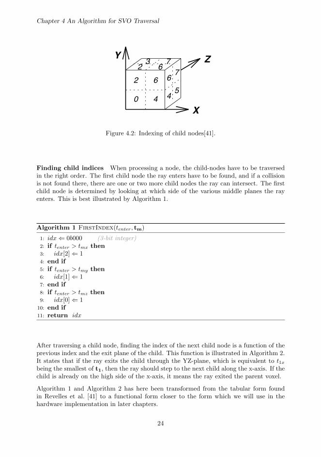
For instance, child 0 in Figure 4.1 is on the left (lower) side of the middle x-plane, andthus its t0x and t1x is the parents t0x and tmx. Determining which side of the middleplane a given child node is on is made easy by carefully selecting the indices of the childnodes. There are 8 child nodes, which can be represented by a 3-bit integer. The childnodes are numbered so that each of the 3 bits determine which side of the middle planethe nodes are on. Bit 2, 1 and 0 represent respectively X, Y and Z. I.e., if bit 2 is set,the child node is on the lower end of the X-axis. This results in the numbering shown inFigure 4.2. The hidden node is node #1.
23
Chapter 4 An Algorithm for SVO Traversal
ZY
X4
67
50
6
4
2
76
32
Figure 1: Labeled octree (the hidden node haslabel 1).
the parent node. If we substitute the following recur-rence relations
(6)
into (4) we obtain
In this case, and are components of the fo-llowing two vectors:
(7)
The last result also holds for . Thus, we haveshown how these values can be incrementally com-puted for all child nodes of the current node. Thecomputation of these values for the root node is car-ried out by using (4).
Knowing the definitions of a node and a ray, we easilydeduce that an intersection between a ray and a nodeoccurs if at least one real value exists such that:
(8)
Where a intersection occurs, an interval o values ofsatisfies the above inequalities. This interval is closedat the left and open on the right for half lines with apositive or zero valued direction vector.
By taking all these results into account, we can nowrewrite the condition 8 by using the parameters of theray. For instance, taking conditionfrom (8), we can substitute by ,then, as is an increasing function, we obtain
. By using the other inequalities in (8) thesame way, we can state that an intersection betweenand occurs if and only if exists such that
(9)
This equation can be further simplified by definingand for a node and a ray as
If a exists obeying (9), then . Theinverse implication also holds, thus equation (9) isequivalent to
(10)
When above condition is true, all values ofin the interval are mapped to points
which belong to the node. If the condi-tion is false, no intersection occurs. It is now possibleto outline the proposed parametric algorithm used totraverse a quadtree. First, we check condition (10) forthe root node. If this condition is not satisfied then theray does not intersect with the octree. But where it is,the four parameters and need to becomputed for the root node by using (4). The main re-cursive procedure is subsequently executed acceptinga node as input parameter, and its corresponding fourparameter values. In cases where the node is termi-nal, this node is added to the resulting pierced nodeslist. If it is non-terminal, those child nodes which arepierced by the ray are checked using (10) for each ofthem. A recursive call to the procedure is carried outfor each of them.
q0 q1
q3q2
tymtx0
ty0
xmt
q0 q1
q3q2tymtx0
txm
ty0
Figure 2: Sub-nodes crossed when(2D case).
q0 q1
q3q2
ttx0y0
txmtym
q0 q1
q3q2
tt
t
xmy0
ym
tx0
Figure 3: Sub-nodes crossed when(2D case).
Note that, for any non-terminal node ,, and . Other child nodes
behave in a similar way. Thus, computation of the en-try and exit parameters for each child node of is re-dundant, because some of them can be taken directlyfrom the parent node, and the others are shared byseveral child nodes. In fact, there are just six different
Figure 4.2: Indexing of child nodes[41].
Finding child indices When processing a node, the child-nodes have to be traversedin the right order. The first child node the ray enters have to be found, and if a collisionis not found there, there are one or two more child nodes the ray can intersect. The firstchild node is determined by looking at which side of the various middle planes the rayenters. This is best illustrated by Algorithm 1.
Algorithm 1 FirstIndex(tenter, tm)
1: idx⇐ 0b000 (3-bit integer)2: if tenter > tmx then3: idx[2]⇐ 14: end if5: if tenter > tmy then6: idx[1]⇐ 17: end if8: if tenter > tmz then9: idx[0]⇐ 1
10: end if11: return idx
After traversing a child node, finding the index of the next child node is a function of theprevious index and the exit plane of the child. This function is illustrated in Algorithm 2.It states that if the ray exits the child through the YZ-plane, which is equivalent to t1xbeing the smallest of t1, then the ray should step to the next child along the x-axis. If thechild is already on the high side of the x-axis, it means the ray exited the parent voxel.
Algorithm 1 and Algorithm 2 has here been transformed from the tabular form foundin Revelles et al. [41] to a functional form closer to the form which we will use in thehardware implementation in later chapters.
24

4.4 Negative Directions and Parallel Rays
Algorithm 2 NextIndex(idxprev, texit-child)
1: idx⇐ idxprev (3-bit integer)2: exit-node⇐ false3: if t1x-child = texit-child then4: if idx[2] = 1 then5: exit-node⇐ true6: end if7: idx[2]⇐ 18: else if t1y-child = texit-child then9: if idx[1] = 1 then
10: exit-node⇐ true11: end if12: idx[1]⇐ 113: else14: if idx[0] = 1 then15: exit-node⇐ true16: end if17: idx[0]⇐ 118: end if19: return idx, exit-node
4.4 Negative Directions and Parallel Rays
Negative Directions It was mentioned that we have assumed that the components ofthe direction vector are all positive. This is obviously not the case for real rays (i.e., a raycan point in any direction in the space), and so the algorithm must be modified slightlyto handle this case. If one of the components of the direction vector is negative, the rayis mirrored about the corresponding middle plane of the octree. Furthermore, a bit maskis set to recall this fact, labeled dir-mask in Algorithm 3. The bit mask is only usedwhen we retrieve a child node. The corresponding bits in the child node index is thenflipped (implemented using xor in Algorithm 3), and the the algorithm will consequentlydescend into the correct child node. Why this works is explained more thoroughly byRevelles et al. [41].
Parallel Rays If a ray runs parallel to an axis, t0 and t1 can not be found (or will beinfinite). There are two ways to deal with this. Revelles et al. [41] suggests setting t0/t1to +∞ or −∞ depending on conditions, and taking this into account in all calculationsthat involve the parameters. A different solution is to check if the components of the raydirection vector d is zero, and if so, set them to a tiny non-zero value[30]. This is slightlyless accurate, but makes the algorithm easier to implement.
4.5 The Tracing Kernel
25

Chapter 4 An Algorithm for SVO Traversal
Algorithm 3 TraceKernel(node, t0, t1)
1: if t1x < 0 or t1y < 0 or t1z < 0 then2: return false3: end if4: tenter ⇐ max(t0x, t0y, t0z)5: if ChildIsLeaf(node) then6: ProcessLeaf(node, tenter)7: return true8: end if9: tm ⇐ (t0 + t1)/2
10: child-idx ⇐ FirstIndex(tenter, t0)11: repeat12: child-node⇐ GetChildNode(node, child-idx⊕ dir-mask)13: t0-child, t1-child ⇐ SelectChildT(child-idx, t0, tm, t1)14: if IsValid(child-node) then15: found-leaf ⇐ TraceKernel(child-node, t0-child, t1-child)16: if found-leaf then17: return true18: end if19: child-node, exit-node ⇐ NextIndex(child-idx, t1-child)20: end if21: until exit-node22: return false
The kernel of the tracing algorithm can now be defined, and is listed in Algorithm 3.It is formulated as a recursive function for clarity. The kernel can be called with theparameters calculated for the root node. It will traverse the octree until a leaf node isfound, or the ray exits the octree. The first lines will skip all nodes it encounters beforethe start of the ray (t = 0). It then checks if the current node is a leaf node. If not, it findsthe first child node index, and starts to iterate over each child node the ray intersects.If a valid node is found it recurses on that node, if not it calculates the next child indexand iterates untill the ray exits the current node.
To illustrate how the algorithm works in practice, Figure 4.3 shows the algorithm runningon a small three-level octree with two solid voxels. The ray will pass close to the firstvoxel and hit the second one.
Initialization The t-values are calculated for the root, and we check if the ray hits theoctree. Since it does, the trace kernel is called for the root node.
Root node The first child index is found (node 0). The child is empty. The next childindex is found (node 2). The child is an inner node. The algorithm recurses on node 2.1©
26

4.5 The Tracing Kernel
0 2 4 6
0 2 4 6 0 2 4 6
0 2 4 6 0 2 4 6
62
0 4
62
0 4
0 2 4 6
0 2 4 6 0 2 4 6
0 2 4 6 0 2 4 6
texit / tstart
62
0 4
62
0 4
620 4
0 2 4 6
0 2 4 6 0 2 4 6
0 2 4 6 0 2 4 6
0 2 4 6
0 2 4 6 0 2 4 6
0 2 4 6 0 2 4 6
0 2 4 6
0 2 4 6 0 2 4 6
0 2 4 6 0 2 64
First child indexNext child index
Enter child node / pushExit child node / pop
Root node
Node 2
Node 2-4
Node 6
Node 6-2
1
2
3
4
5
6
Figure 4.3: Illustration of the octree tracing algorithm.
Node 2 The first child index is found (node 4). The child is an inner node. Thealgorithm recurses on node 2-4. 2©
Node 2-4 The first child index is found (node 0). The child is empty. The next childindex is found (node 4). The child is empty. The next child index is found (node 6). Thechild is empty. The ray exits the current node and the algorithm goes up a level. If weused a restarting algorithm, we would use texit-child to set a parameter tstart, and restartfrom the root. Then, when evaluating a node, we would pass it if tenter < tstart. 3©
Node 2 We re-enter node 2 from child index 4. The ray exits the current node and thealgorithm goes up a level. 4©
27

Chapter 4 An Algorithm for SVO Traversal
Root node We re-enter the root node from child index 2. The next child index is found(node 6). The child is an inner node. The algorithm recurses on node 6. 5©
Node 6 The first child index is found (node 2). The child is an inner node. We recurseon node 6-2. 6©
Node 6-2 The first child index is found (node 0). The child is empty. The next childindex is found (4). The child is a solid voxel. The algorithm terminates.
28

Chapter 5
A Ray Tracer Geometry Stage
With traditional rasterization, the model-view matrix and the perspective projectionmatrix is the main data which dictates the size and position of the models relative to thecamera, and how they should be projected to a 2D image. If ray tracing of SVOs is tobe implemented alongside rasterization, it would be very benificial to use the same datain the ray tracer. This chapter outlines a geometry stage for a ray tracer which mirrorsthe one used in rasterization. Although it is probable that these techniques have beendeveloped previously, for instance in commercial ray tracing systems, it was not describedin any of the literature covered in this thesis. Therefore, these techniques were developedindependently.
5.1 Normalizing the Octree
In rasterization, the world is transformed so the camera occupies a fixed position andorientation, and the volume that should be rendered occupies a fixed space. With raytracing of sparse voxel octree, it is the octree that must occupy a fixed position. Asmentioned, the algorithm requires an axis-aligned octree. The algorithm can in principlework with an octree of any size. However, to simplify analysis and implementation, wechoose to normalize the octree so that it occupies the volume defined that by the points(-1,-1,-1) to (1,1,1). I.e., the length of the sides of the octree is always 2, and the centerof the octree is in the origo of the coordinate system. Instead of defining the size and theposition of the model by the corners of the octree, we can use a model transform matrix.This has two benefits: the core of the algorithm can make simplifying assumptions, andthe same techniques used to transform polygon model can be used to transform the octree,which should simplify and ease programming.
29

Chapter 5 A Ray Tracer Geometry Stage
5.2 Generating Primary Rays
In a ray tracer, it is the position and direction of the primary rays which dictates how themodel end up looking on the screen. We can easily define these rays in the canonical viewvolume. Each ray starts at z = −1 and ends at z = 1, and they are evenly spaced alongthe X/Y axis. The distance between each ray along the X and Y axis is defined by thewidth and height of the image. Now consider the transforms discussed in Chapter 2.2. Ifwe follow these in reverse, we get the position and direction of the rays in the coordinatesystem where the octree is axis aligned and normalized. In essence, the idea of the raytracer geometry stage is to perform the same operations as in the rasterization geometrystage (Figure 2.3), and perform them in reverse on the ray data rather than the modeldata. This is illustrated in Figure 5.1. Fortunately, the model and view transform canbe reversed simply by taking the inverse of the model/view matrix, but the perspectiveprojection transform requires some elaboration.
x
z
x
z
x
z
x
z Octree
Inverse Model TransformInverse View TransformInverse Projection Transform
Image / Screen
Rays
the X/Y axis. The distance between each ray along the X and Y axis is defined by thewidth and height of the image. Now consider the transforms discussed in Chapter 2.2. Ifwe follow these in reverse, we get the position and direction of the rays in the coordinatesystem where the octree is axis aligned and normalized. In essence, the idea of the raytracer geometry stage is to perform the same operations as in the rasterization geometrystage (Figure 2.3), and perform them in reverse on the ray data rather than the modeldata. This is illustrated in Figure 5.1. Fortunately, the model and view transform canbe reversed simply by taking the inverse of the model/view matrix, but the perspectiveprojection transform requires some elaboration.
Octree
Inverse Model TransformInverse View TransformInverse Projection Transform
Image / Screen
Rays
Figure 5.1: A ray tracer geometry stage in action
Equation 5.1 shows the equations for the ray tracer geometry stage, where x and y arethe x and y coordinates of the pixel in the image, w and h is the width and height of theimage, v0 and v1 are the starting and end point of the ray in the canonical view space, q0,q1, p0 and p1 are the same points in the camera space and the normalized octree space,Pi is the inverse perspective projection and Mmv is the model-view tranform matrix.
v0 = (x/w, y/h,�1, 1)
v1 = (x/w, y/h, 1, 1)
q00 = Piv0
q01 = Piv1
q0 = q00/q
00w
q1 = q01/q
01w
p0 = Mmv�1q0
p1 = Mmv�1q1
(5.1)
The ray origin o and direction vector d for the ray traversal algorithm (see Equation 4.1)may be found as such:
o = p0
d = p1 � p0
(5.2)
26
Figure 5.1: A ray tracer geometry stage in action
Equation 5.1 shows the equations for the ray tracer geometry stage, where x and y arethe x and y coordinates of the pixel in the image, w and h is the width and height of theimage, v0 and v1 are the starting and end point of the ray in the canonical view space, q0,q1, p0 and p1 are the same points in the camera space and the normalized octree space.These points are also illustrated in Figure 5.1. Pi is the inverse perspective projectionand Mmv is the model-view tranform matrix.
v0 = (x/w, y/h,−1, 1)
v1 = (x/w, y/h, 1, 1)
q′0 = Piv0
q′1 = Piv1
q0 = q′0/q′0w
q1 = q′1/q′1w
p0 = Mmv−1q0
p1 = Mmv−1q1
(5.1)
30

5.3 Inverse Perspective Projection
The ray origin o and direction vector d for the ray traversal algorithm (see Equation 4.1)may be found as such:
o = p0
d = p1 − p0
(5.2)
5.3 Inverse Perspective Projection
The model/view matrix can be inverted using standard matrix inversion algorithms suchas Gauss-Jordan elimination. The perspective projection however, can not be inverted bysimply inverting the perspective projection matrix, because the result is divided by thew -component(Equation 2.4). Using simple linear algebra, we can find a similar equationto go from a canonical view space point v to a camera space point q.
Solving for Pi results in the following matrix:
Pi =
− f(r−l)
f−n 0 0 − f(r+l)f−n
0 − f(t−b)f−n 0 − f(t+b)
f−n0 0 0 2fn
f−n0 0 1 − f+n
f−n
(5.3)
5.4 Normalizing Ray Length
A ray has a starting point and a direction. The direction is often defined as a normalizedvector with a length of 1. However, the output of the proposed geometry stage is a startingpoint and an end point. The starting point is positioned at the near plane and the endpoint is positioned at the far plane. Although a far plane is strictly speaking not necessaryin a stand-alone ray tracer, when combining with rasterization it can be be useful to havethe option of terminating the ray tracing at the far plane. Following equation 2.5, thenear plane is placed at t = 0 and the far plane at t = 1. If we standardize on this, ouralgorithm can be designed to optionally terminate at t = 1. This functionality should beuseful when calculating light/shadow rays as well. In this case we also have a startingpoint (the point at which the primary ray hits an object) and an end point (the lightsource), and we are only interested in finding if the line between these points intersectssome object. I.e., we should terminate the ray tracing at t = 1. Another useful feature ofhaving the start and end point be at the near and far plane, is that the resulting t-valuecan be used to calculate a value for the Z-buffer.
5.5 Z-Buffering With Ray Tracing
In rasterization, the Z-buffer ensures that the geometry appears appears in the correctorder from front to back. If we wish to merge the result of the ray traced image with a
31

Chapter 5 A Ray Tracer Geometry Stage
rasterized image, and have everything appear in the correct order, we need to be able togenerate the correct values for the Z-buffer.
When a primary ray hits a voxel, the algorithm returns a t-value (tout) which representhow far along the ray the voxel is. Because we placed the start and end of the ray at thenear and far plane, this t-value also represents the position of the voxel between the nearand the far plane. This is illustrated by the red dot in Figure 5.1, which can be followedin reverse from its position in the octree on the right, to its position in the canonical viewvolume on the left.
However, this can not be directly used as a Z-value. The tout is linear with regards todistance in the camera space. In rasterization the Z-value is linear with regards to distancein the canonical view volume. If we use perspective projection, this Z-value is not linearwith regards to camera space. If we look at Equation 2.4, we can see that the Z-valuein the canonical view volume, vz, is divided by v′w. This implies that vz is a function of1/qz where qz is the Z-value in the camera space.
To solve this problem, we can first find the collision point in the camera space, given thet-value at the collision point tout:
qc = q0 + (q1 − q0) · tout (5.4)
Using the perspective projection matrix Pp defined in Equation 2.3, we can transformthis coordinate in to the canonical view volume:
vc = Ppqc (5.5)
Taking the z-coordinate from this vector will give us a Z-value which is compatible withthe Z-buffer generated by the rasterizer.
32

Chapter 6
Hardware Optimizations
In order to optimize the ray traversal algorithm for hardware implementation, variousconsiderations were made, and the algorithm was transformed to a form which is feasibleto implement in a hardware description language. This chapter will present the rationalefor using fixed point numbers, we will analyze the use of a stack in hardware, and thefinal hardware optimized version of the algorithm will be presented.
6.1 Floating Point vs Fixed Point
A fundamental decision regarding how to implement the algorithm, was whether to usefloating point or fixed point representation for the parameters in the algorithm. Sincethe algorithm could be integrated with a modern GPU – which extensively support useof floating point numbers – using a floating point representation might be pertinant.However, looking at the algorithm, the operations performed on the parameters in thecore of the algorithm are only additions and divisions by two. Additions require muchmore resources to implement and is slower to execute with floating point numbers. Thedifference is probably even more dramatic with the division by two. This can be donewith a simple sign-extended shift operation in fixed point arithmetic[26]. Because of thesedifferences in resource use, a fixed point representation was chosen in this thesis.
To integrate the hardware module presented in this thesis with a system using floatingpoint numbers, the module could integrate a floating point to fixed point conversion unit.Even given the cost of this unit, it is probably still better than using floating point unitswithin the core of the module. The floating point parameters passed to the module couldfall out of range of the chosen fixed point representation, but this could be solved byscaling the parameters by a common factor such that the largest parameter falls withinthe range of the fixed point representation. When the results are passed back out of themodule, they could be scaled back using the same scaling factor.
The number of bits used to represent the number was chosen to be 32 bits. This was dueto the fact that the bus width is 32 bits, and that the OpenRISC processor that was used
33

Chapter 6 Hardware Optimizations
is a 32-bit processsor.
6.2 The Decimal Point
The position of the decimal point in a fixed point number dictates the range and precisionof the numbers that can be represented. In this thesis, it was decided to use 16-bit eachto represent the integer and fractional part of the number. Since the octree is normalizedto exist within the range −1..1, the octree is contained within the fractional part of thenumber. Consequently we have 16 bits to represent a position within the octree.
Numbers equal to or larger than 215 can not be represented by the chosen representa-tion. When calculating the initial t-values for the algorithm, it is important to makesure the calculations to not overflow, which would make the results nonsensical. Tak-ing Equation 4.1 and applying the constraints of the normalized octree, we end up withEquation 6.1, where ox and dx is x-component of the ray origin and direction vectors.
t0x = (−1− ox)/dx
t1x = (1− ox)/dx(6.1)
Assuming the ray origin is somewhere outside the octree, i.e. ox � 1, we have t0x ≈ ox/dx.The value of t0x can easily overflow if ox is large and dx is small. We should therefore puta constraint on ox. Constraining ox arbitrarily to be less than 25 gives us a lower boundfor dx:
dx = ox/t0x = 25/215 = 2−10 (6.2)
This implies that if 2−10 < dx < −2−10, then dx should be clipped to ±2−10 beforecalculating t0 / t1. If we do this we also avoid the problem discussed in Chapter 4.4,where dx = 0. This clipping implies there is a limit to the resolution of the directionvector, and we have shown that there is a relationship between this limit, the maximumvalues of the origin vector and the upper bound of our number representation.
6.3 Stack
Algorithm 3 is formulated as a recursive function. Since functions are not a native primi-tive in hardware design, an explicit stack must be used to achieve the same functionality.Instead of recursing, the algorithm will push the necessary variables in the stack, andinstead of returning the variables will be popped from the stack.
The stack requires memory, and since the purpose of the stack is to avoid slow memoryrequests, the stack memory should be fast, preferably accessible in one clock cycle. Thisimplies that this memory will be expensive in terms of resources, and we should seek tominimize the size.
34

6.3 Stack
The state that must be stored on the stack are the node data and address, the currentchild index, and the t-values t0 and t1. The node address is a 32-bit pointer pointing tothe node data. The node data is a 32-bit value consisting of the 16-bit child table pointerand the 16-bit child data. The node data is not strictly necessary since we could requestthe node data from memory using the node address. Howevery, this would partly defeatthe performance enhancing benefits of the stack.
It is possible to eliminate the need to store the 16-bit child pointer on the stack. Wheneverthe algorithm enters a child node, we must calculate the child address. Taking the currentnode address and adding the 16-bit child table pointer gives us the address of the table ofchild nodes. Adding the child offset to this value gives us the address of the desired childnode. By storing the resolved child node table address instead of the parent node addresson the stack, we avoid the need to store the child table pointer, as the only use of thesetwo values is to calculate the child table address. This optimization has a secondarybenefit aswell: if the child table pointer is a far pointer, we need to perform an extramemory request to fetch the far pointer in order to calculate the child table address. Bystoring the child table address on the stack we avoid having to resolve the far pointeragain later.
The child index is a 3-bit value. It is not strictly necessary to store this value on the stack.If we implement restarting, as will be described later, the tstart parameter is sufficient toinsure that we do not visit nodes we have visited before. However, this would come at acost of a few extra wasted clock cycles each time the stack is popped. Considering thatthe child index is so small relative to the node data/address, it is probably worth keepingon the stack.
The t-values t0 and t1 are each a vector of three 32-bit numbers. However, it is notnecessary to store the full value of these numbers on the stack. When the algorithmenters a child node, the t-values for the child node is picked from t0, tm and t1. If wecan reconstruct the parents t-values from the child t-values we can avoid storing them onthe stack. Consider how the child t-values are calculated:
tm = (t0 + t1)/2 (6.3a)
t0x-child = t0x
t1x-child = tmx
}If child-idx[2] is 1 (6.3b)
t0x-child = tmx
t1x-child = t1x
}If child-idx[2] is 0 (6.3c)
If we store child-idx on the stack, we can use this value to find either t0x or t1x. We callthis value tpass:
tpass = t0x = t0x-child
tmx = t1x-child
}If child-idx[2] is 1 (6.4a)
35

Chapter 6 Hardware Optimizations
tpass = t1x = t1x-child
tmx = t0x-child
}If child-idx[2] is 0 (6.4b)
The other value, which we will name trecover, must be recovered from tmx. However, thedivision by two in Equation 6.3a, which is implemented as a shift-operation in hardware,discards one bit of information. To recover trecover, we need to save this bit, which wewill call tbit.
tmx, tbit = (tpass + trecover)/2 (6.5a)
trecover = (tmx, tbit) · 2− tpass (6.5b)
Finally we set t0x or t1x to trecover depending on the value of child-idx[2].
Using this method, we have reduced the stack memory requirement of the t-values toone bit per component, i.e., three bits in total. Adding up the total size of the requiredvariables we get 32 + 16 + 3 + 3 = 54 bits. For a stack of depth D the total size of thestack in bits S is:
S = 54D (6.6)
The optimal depth of the stack, and thus the total size of the stack, has been optimizedexperimentally. This is presented in Chapter 8.
6.4 Restarting
Implementing restarting is useful because it makes it possible to trace octrees which aredeeper than the depth of our stack. We can adjust the size of the stack to a size that givesthe best performance for the resources we use, and we do not have to worry about thesize of the octree. Even if the stack is large enough to trace the octrees we are currentlyusing, we might want to use the hardware for larger octrees in the future.
First, we need to find the t-value at which the ray exits a node:
texit = min(t1x, t1y, t1z) (6.7)
Restarting requires one extra variable tstart. When we exit a node, instead of popping thestack to return to the parent node, we store texit in tstart. We then restart the algorithmfrom the root node. Each time the algorithm processes a child node it will pass the nodeif tstart >= texit−child. I.e., the next time we visit the parent node of the last node wevisited before we restarted, the algorithm will pass that node.
36

6.5 Hardware Optimized Algorithm
This operation is quite expensive compared to popping the stack, since we have to processevery node from the root node down to the parent node of the node we exited, while whenwe pop the stack we go directly back to the parent node.
6.5 Hardware Optimized Algorithm
To implement the raytracing algorithm in hardware, it first had to be converted to a formwhich is suitable for hardware implementation. The goal was to create a state machinewhere the operations performed in each state was limited and reuse of functional unitswas possible between states. This process did not follow a strict methodology, but it wasinformed by techniques from high-level synthesis[12] and compiler techniques[2].
First, the kernel listed in Algorithm 3 was changed from a recursive form to a non-recursiveform. The recursive function call was replaced by a loop and a stack was introduced whichcould save and restore the required state, after which the algorithm consisted of a set ofnested loops. The algorithm was converted to a state machine by introducing a state foreach basic block in the function, and replacing loop branching with state transitions.
In synchronous digital circuits, it is important to keep the delay of the critical path(i.e., the longest path through a combinatorial circuit) below the period of the clock. Ashorter critical path increases the maximum clock frequency of the design. This can beachieved through pipelining, which splits the critical path with registers, and the sameoperation is divided over additional clock cycles[4]. In this thesis the algorithm wasimplemented in a system alongside the 32-bit OpenRISC processor and the ray tracingmodule was designed to run at the same clock frequency as this processor. Running themodule and the processor at different clock frequencies would have resulted in a designwith multiple clock domains which are more difficult to implement[4]. The OpenRISCprocessor performs 32-bit addition, subtractions and comparisons in one clock cycle[36].To keep the maximum clock frequency of the ray tracing module similar to that of theprocessor, the algorithm was designed so that the critical path would go through no morethan one 32-bit adder/subtractor/comparator, a couple of multiplexer and some simplecombinatorial logic. To achieve this, any state that had two or more chained arithmeticoperations was split into two or more states.
To minimize the amount of resources a digital design uses, it is important to consider re-source sharing. By allowing the operations in different states to share functional units suchas arithmetic units, we can minimize the area (or LUTs) consumed by the design[40]. Sev-eral operations in the presented algoritm requires three comparators. These are the max,min and FirstIndex(Algorithm 1) functions in Algorithm 4. These are all performed indifferent states, and could potentially share comparators. As adders and comparators aresimilar functional units, the calculation of tm could potentially also share these units, bysplitting up the CalcT state. Even further reduction of resource use could be achievedby further pipelining the design and perform a single addition/comparison in each cycle.
Algorithm 4 shows the kernel of the algorithm converted to a form which should besuitable for hardware implementation. Each label represents a state in a state machine,and each state has been assigned operations that can be executed in a single cycle. Thisalgorithm was used in the ray traversal core of the hardware implementation. Further
37

Chapter 6 Hardware Optimizations
descriptions along with a state diagram can be found in Chapter 8.5.
Algorithm 4 TraceCore(root-adr, root-t0, root-t1, dir-mask)
1: globals node, level, idx2: globals is-first-node, exits-node, pass-node3: globals t-start, t-enter, t-exit, t-exit-child4: globals t0, t1, tm, tbit5: globals t0-child, t1-child6: globals is-leaf, t-out7: Init:8: t0 ⇐ root-t09: t1 ⇐ root-t1
10: is-first-node ⇐ true11: level ⇐ 012: node ⇐ GetRootData(root-adr)13: goto CalcT
14: CalcT:15: tm, tbit ⇐ (t0 + t0)/216: t-enter ⇐ max(t0x, t0y, t0z)17: if is-first-node then18: goto FirstIdx19: else20: goto NextIdx21: end if
22: FirstIdx:23: if got-node-data then24: idx ⇐ FirstIndex(t-enter, tm)25: exits-node ⇐ false26: is-first-node ⇐ false27: goto CalcChildT28: else29: goto FirstIdx30: end if
38

6.5 Hardware Optimized Algorithm
TraceCore continued
31: NextEval:32: idx, exits-node ⇐ NextIndex(idx, t-exit-child)33: if exits-node then34: if level = 0 then35: is-leaf ⇐ false36: t-out ⇐ t-exit-child37: goto Finished38: else if stack-empty then39: t-start ⇐ t-exit-child40: goto Init41: else42: node, t0, t1, idx ⇐ Pop43: level ⇐ level− 144: goto CalcT45: end if46: else47: goto CalcChildT48: end if
49: CalcChildT:50: t0-child, t1-child ⇐ SelectChildT(idx, t0, tm, t1)51: t-exit-child ⇐ min(t1x−child, t1y−child, t1z−child)52: goto Eval
53: Eval:54: pass-node ⇐ t-exit-child <= t-start55: if pass-node then56: goto NextIdx57: else if IsChildLeaf(node, idx⊕dir-mask) then58: t-out ⇐ t-enter59: goto Finished60: else if IsChildValid(node, idx⊕dir-mask) then61: Push(node, tbit, idx)62: t0 ⇐ t0-child63: t1 ⇐ t1-child64: level ⇐ level + 165: is-first-node ⇐ true66: node ⇐ GetData(node, idx⊕dir-mask)67: goto CalcT68: else69: goto NextIdx70: end if
71: Finished:72: return is-leaf, t-out
39

Chapter 6 Hardware Optimizations
40
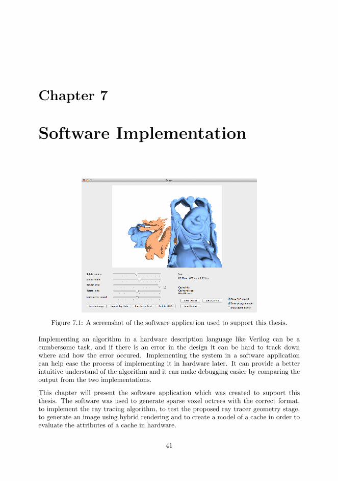
Chapter 7
Software Implementation
Figure 7.1: A screenshot of the software application used to support this thesis.
Implementing an algorithm in a hardware description language like Verilog can be acumbersome task, and if there is an error in the design it can be hard to track downwhere and how the error occured. Implementing the system in a software applicationcan help ease the process of implementing it in hardware later. It can provide a betterintuitive understand of the algorithm and it can make debugging easier by comparing theoutput from the two implementations.
This chapter will present the software application which was created to support thisthesis. The software was used to generate sparse voxel octrees with the correct format,to implement the ray tracing algorithm, to test the proposed ray tracer geometry stage,to generate an image using hybrid rendering and to create a model of a cache in order toevaluate the attributes of a cache in hardware.
41

Chapter 7 Software Implementation
The application was created using Xcode on Mac OS X. The GUI-related code was writtenin Objective-C, while the code to generate and trace the octree was written in C++. Thesoftware was executed on a laptop with a 2 GHz Intel Core i7 processor, 4 GB of 1333 MHzDDR3 memory and an AMD Radeon HD 6490M GPU with 256 MB graphics memory.
7.1 SVO Data Structure
Both the software and hardware implementation needs data in a sparse voxel octreeformat. The data structure in this thesis is organized in a way similar to that of Laineand Karras [29], but the contour data, page header and info section they describe wasdropped as none of those features was required for this thesis. The resulting data structureis illustrated in Figure 7.3. The data structure is an array of 32-bit entries. Two 8-bitmasks indicate the type of the child nodes. The 8-bit leaf_mask indicates whether achild node is a leaf node or not. The 8-bit valid_mask indicates whether a child nodehas solid voxels or not. A partially filled inner node will have its valid_mask set but notits leaf_mask. A solid leaf node (a solid voxel) will have both set. If the node has anyinner node children, the 15-bit child_table_ptr is a relative pointer to a table of thesechild nodes. If the 15-bits are not enough to hold the pointer, the is_far bit is set, andchild_table_ptr points to an entry with a 32-bit pointer. The final address of the childtable is found by adding the 32-bit far pointer to the parent node address.
000000001000100000000000000000100 (root)
leaf_maskvalid_maskchild_table_pointeris_far
000000001000010100000000000001101000000000101000000000000000000112
3
000001010000010100000000000000004000101000001010000000000000000005111000001110000000000000000000006
110000001100000000000000000000007000000110000001100000000000000008
address15 bits 8 bits 8 bits
32 bits
00000000000000000000000000000101
Root
0 1 2 3 4 5 6 7
0 1 2 3 4 5 6 7 0 1 2 3 4 5 6 7
Figure 7.2: The organization of the sparse voxel octree data structure.
7.2 Generating Sparse Voxel Octrees
The models used in this thesis was the “Stanford Bunny”, “Happy Buddha” and “StanfordDragon” models from Stanford Computer Graphics Laboratory [50]. These models wereprocessed by the third-party program “binvox”[16], which converted the polygon modelsto voxel models. The program outputs a run-length encoded voxel format. A routine
42

7.3 Software Ray Tracer
was created to convert this format to an octree. The routine loads the entire voxel modelto a three-dimensional array in memory. It then recursively divides the array into eightsub-regions untill a region contains a single voxel and constructs an inefficient octree inthe process. This octree is then compacted into the binary format described previously.This data can then be used by the software application and be written to a binary filewhich can be uploaded to the FPGA memory. The voxel models are 1024 voxels widealong each axis, and the resulting octree is 10 levels deep.
dragon.ply33.8MB
Polygon Model
binvox
dragon.binvox9.4MB
Run-length encodedvoxel array
OctreeConverter
dragon.bin2MB
Sparse Voxel Octree
Figure 7.3: The process of generating sparse voxel octree models.
7.3 Software Ray Tracer
The ray tracing algorithm was implemented in software to provide reference images andfacilitate in debugging the hardware solution. Initially the algorithm was implementedaccording to Algorithm 3, but it was later rewritten to closely match the hardware version.This proved immensely useful in debugging. When rendering the same image using thesame input, the software and hardware simulation could be executed and the value of thevariables in the algorithm could be compared at different points during execution. Thismade it easier to locate and fix bugs in the hardware implementation. The software raytracer was also used to generate the parameters required to initialize the ray tracing corein the hardware implementation. The same function which generates these parametersfor the ray tracing kernel in software can be redirected to write these parameters to afile. This file can then be uploaded to the FPGA memory and used by the hardware raytracing core.
There are some important differences between the software and the hardware ray tracer.The software version does not run on multiple cores in parallell. It can use either floatingpoint numbers or fixed point numbers in the calculation. Furthermore, although botha stack and cache is implemented in the software version, they are used to simulate thebehavior of the hardware version, not to boost the performance in software. Finally, theshading, i.e., the coloring of the rendered image is different. In the software implementa-tion, simple hard shadows are rendered by tracing secondary rays from the collision pointof the ray to a point light source. These shadows are used to better visualize the octreemodel, and to provide preliminary indications that such techniques are possible using thealgorithm. The software can also visualize the cost of rendering a ray by coloring the
43

Chapter 7 Software Implementation
pixel of the ray according to the number of memory requests required to trace that rayas seen in Figure 7.5
The core functions of the code for the software ray tracer is included in the appendix.
7.4 Merging Ray Tracing and Rasterization
To test the proposed technique for merging ray tracing and rasterization, the software raytracer was designed with the proposed geometry stage, and the corrected Z-values wasextracted and stored in a Z-buffer. The GPU on the computer executing the softwarewas utilized through the OpenGL API to perform rasterization. The dragon voxel modelwas rendered with the ray tracer and the resulting image and Z-buffer was uploaded tothe image buffer and Z-buffer of the GPU. The bunny and buddha polygon models werethen drawn using the GPU, positioning them such that the bunny would appear behindthe dragon, and the buddha in front of the dragon, if the Z-buffer generated by the raytracer was correct. The results from this experiment is illustrated in Figure 7.4. It showsthe image and depth buffer from the octree ray tracing and polygon rasterization, andthat the three models appear in correct order in the combined image.
+
=
Figure 7.4: Ray traced image and Z-buffer + rasterized image and Z-buffer = combinedimage and Z-buffer
7.5 Cache Profiling
It was suspected that the memory bus of the hardware module would be a bottleneck forthe algorithm. To investigate the benefits of a data cache in the hardware implementationa behavioral model of a cache was created in software. Each access to a node or far pointerin the octree was logged by a software cache model. This cache has three configurations:the cache size (in number of 32-bit words), the block size (in words) and block placementpolicy (direct mapped and 2/4-way set associative). A small test routine rendered a givenSVO model from four different angles, logged the cache hits/misses and calculated theaverage miss rate.
As the data cache is designed for a specific algorithm, it should in theory be possible
44

7.5 Cache Profiling
to implement novel and specific optimizations to the cache which exploits the memoryaccess patterns of the algorithm. For instance, nodes that are closer to the root are morelikely to be accessed often than nodes deeper in the tree. It is possible that it is inefficientto cache nodes deeper in the tree. If they are accessed only once or twice, the benefit ofcaching them is small compared to the penalty of evicting a node closer to the root. Toinvestigate this, a cache model was created where the cache was given the level of thenode accessed in addition to its address. The cache could then be configured to disablecaching for deeper nodes.
45

Chapter 7 Software Implementation
7.6 Results
Direct mapped
Block size
Cache size 1 2 4 8
32 0.46 0.54 0.60 0.61128 0.25 0.28 0.31 0.33512 0.17 0.17 0.16 0.16
Two way set associative
Block size
Cache size 1 2 4 8
32 0.37 0.49 0.60 0.60128 0.18 0.19 0.21 0.26512 0.14 0.12 0.10 0.09
Four way set associative
Block size
Cache size 1 2 4 8
32 0.31 0.45 0.60 0.59128 0.15 0.14 0.16 0.20512 0.14 0.11 0.08 0.06
Two way set associative1 word block size
Cache size
Max level* 8 32 128 512
2 0.66 0.53 0.48 0.474 0.67 0.43 0.31 0.286 0.70 0.40 0.24 0.178 0.72 0.42 0.24 0.18
*Max level of N: only the nodes N levels orless from the root are cached
Table 7.1: Cache miss-rate results from software profiling. Smaller numbers are better.
Figure 7.5: An illustration of the cost of tracing the primary rays. The lighter the colorthe more memory requests was used to trace that ray.
46

7.7 Discussion
Stanford Bunny Stanford Dragon Happy Buddha652ms 824ms 677ms
Figure 7.6: The three voxel models and their rendering speed in software.
7.7 Discussion
In the few experiments that were done, merging ray tracing and rasterization using theZ-buffer seemed to work correctly. In addition, since the model-view transform matricesused in ray tracing was extracted from the OpenGL API, the same OpenGL calls thatwere used to set up the rasterized models could be used for ray tracing as well. Thesame function calles used to set up the camera for the OpenGL rasterizer was used forthe ray tracer as well. In other words, programming was made easy and tidy. However,this is a very basic demonstration. Commercial games rely on many different effects, e.g.,translucent materials, reflections and shadows. Implementing these various effects usinga hybrid rendering technique will probably be challenging.
The cache profiling resulted in some interesting data. Larger block size has a negativeimpact on the performance of the cache for small cache sizes. However, for large cachesizes the cache miss-rate seems to improve with larger block sizes, especially with twoand four way set associative caches. It is possible that there is a rather small chance thatthe next memory access is one of the other words in the block. For small cache sizes thatcould imply that it is more likely that the algorithm will need one of the words that hadto be evicted, than one of the other words in the block. However, as the cache size grows,the probability that a cache block read will evict a word that the algorithm will soonaccess diminishes.
A two way set associative cache is better than a direct mapped cache, and two way isbetter than four way. However, the improvement from two way to four way set associativeis minor, and might not be worth the increased resources required to implement it. Finally,restricting which words are cache based on the depth of the node which is accessed seemsto be detrimental to performance, for all but the very smallest caches. To understandwhy, consider the case where the ray for one pixel has been traced. The cache is nowfilled with nodes from this trace. In this implementation the next pixel to be traced isthe next pixel to the right in the image. When tracing the ray for this pixel, it will followa path very similar to the one for the last pixel, and consequently it will access mostlythe same nodes, even for nodes deep in the tree. However, secondary rays such as thoseused to calculate shadows and reflections, are not as coherent as the primary rays. Thereis a possibility that a variation of this optimization could be useful in a more complexrendering system.
47

Chapter 7 Software Implementation
Figure 7.6 shows the time it took to render the three models in software. These are givento provide some frame of reference to the results from the hardware implementation.Because neither implementation is aggressively optimized, and given the vast differencesin hardware capabilities, a direct comparison is of little interest. However, it wouldbe surprising if the relative speed from one model to the others is different in the twoimplementations. Note that the dragon model takes longer to render. If a ray passesclose to the edge of a model, it will be costly to trace because it will have to traversedeep in the octree to determine if it collides with a voxel or not. This effect is illustratedeffectively in Figure 7.5, where brighter colors imply higher cost. Although the dragonappears to have a similar surface area as the bunny, the edge has more folds, and thus ismore costly to render. In this figure one can also observe the structure of the octree. Asthe ray crosses into new octants the cost increases, and thus faint cubes can be observedin the picture.
48

Chapter 8
Hardware Implementation
The goal of this thesis was to create a practical design for ray tracing of sparse voxeloctrees in hardware. To demonstrate that the proposed design could work, a hardwareprototype had to be created. An FPGA prototype board was used, and a system-on-chipplatform for that board was modified to include a ray tracing module. This module waswritten in the Verilog hardware description language.
This chapter presents the design of the hardware system and the details of the designof the ray tracing modules and its sub-components. The methodology used to test thecomplete system is presented, along with the results. Finally, the design and results arediscussed.
8.1 Hardware Platform
As one of the goals of the thesis was to synthesize the module for an FPGA, a prototypeboard had to be chosen. The criteria for selecting an FPGA prototype board was:
• Academic Discount
• On-board RAM for storing ray data, octrees and the resulting image
• Video output (VGA or DVI/HDMI)
The Digilent Atlys prototype board was selected since it fitted well with the chosencriteria. One drawback of the board is that it contains relatively few switches and LEDs,and no display. However, there is a USB-port for a keyboard and/or mouse, and thereis UART over USB. The UART module has been used extensively to debug the system,by communicating with a terminal on a personal computer. Additionally, the Cypressmicrocontroller that is used to configure/program the FPGA over USB, also connects tothe FPGA through a set of data signals. Digilent provides a software API and a piece ofsoftware to transfer data to the FPGA over these signal lines.
49

Chapter 8 Hardware Implementation
Two different architectures was considered for the thesis. One was a standalone system,where the system would consist of only the ray tracing module, and the necessary supportto connect it to RAM, to initiate ray traing, and to get image out to a computer or adisplay. The second was to use a soft core CPU, and implement the ray caster as anaccelerator. A soft core CPU is a CPU which can be implemented on an FPGA[46],while an accelerator is a component attached to the same bus as the CPU which canprovide performance increases for specific functions[63]. The benefits of having a CPU isthat some parts of the system can be significantly easier to implement in software thanin hardware. If those are not performance critical, then having a CPU to perform thosetasks can cut down design time with little or no performance penalty. However, a softcore CPU can take up a significant amount of the FPGAs resources, leaving less for theray tracing module, and increasing the time it takes to synthesize the system.
Computer
Pear NoteBook Pro
or1200OpenRISC CPU
Wishbone /DDR RAM Interface
Instruction Bus
Data Bus
Byte Bus
Master Master
Bridge Master
Slave (R)
128MbyteDDR2 RAM
Slave (R/W)
Ray Tracing Module
SlaveMaster
Slave (R/W) Slave (R) Slave (R/W)
ROM
Slave
SPI
Slave
UART
Slave
GPIO
Slave
16MbyteSPI Flash
ButtonsSwitches
LEDs
orlinkPC/FPGA
Link
Master
USB I/F USB I/F
VGA/HDMIEncoder
SlaveMaster
Digilent Atlys Prototype Board
Xilinx Spartan-6FPGA Chip
Modules implemented in this thesis
ORPSoC Modules
Board peripherals/ICs
Display
Figure 8.1: Hardware platform overview
The second architecture, with a CPU and the ray caster implemented as an accelerator,was chosen because the complexity of creating a stand-alone system was deemed to be toomuch for this thesis, and that debugging the system could be hard without an internalCPU which could quickly be programmed to change certain behavior in the system. Tocreate the proposed system an existing system-on-chip solution had to be found. Therewas some investigation into using Xilinx’ embedded development kit (EDK) and theirMicroBlaze CPU. However, the tools were complicated to use and did not encourageautomating the synthesis of the design. The open source system-on-chip solution ORPSoChas recently been ported to Atlys by Kristiansson [27]. Using this platform as a basis forthe project meant that all the support modules were already in place. The ray tracing
50

8.2 Ray Casting Module
module could easily be attached to the system bus, using the open interface standardWishbone. In addition, the complete system could be built using Makefiles, which impliesthat the process of synthesizing the design could easily be automated, allowing manyvariations of the design to be synthesized.
A module named orlink was also created for this thesis. This module supports transfersbetween a computer and the FPGA system. This allowed OpenRISC software, ray dataand octree data to be uploaded to the on-board RAM, and the resulting image to bedownloaded to a computer. This work builds on McClelland’s FPGALink [32] software,which uses a custom firmware for the Cypress microcontroller on the board. The softwarepresents a software API similar to the one Digilent provides. However, FPGALink iscross-platform and open-source. Orlink consists of a verilog module, and a piece ofsoftware. The Verilog module translates request from the microcontroller, to Wishbonebus requests. The orlink software is a command-line interface that allows a user to haltand reset the CPU on the FPGA and transfer data between a personal computer and theon-board memory. As the module is not directly relevant to the results of the thesis, thedetails of this module will not be presented.
The final system is presented in Figure 8.1. The OR1200 OpenRISC CPU uses a Harvardarchitecture, which is why there is a separate instruction and data bus. The ROM moduleis a small read-only memory on the FPGA, which bootstraps the CPU. The bootstrappercan load software from an SPI Flash chip, or it can simply cause the CPU to jump toa reset vector in RAM. Both of these modes have been used in the project for variouspurposes. The instruction bus and the data bus are 32-bits wide, while the byte bus is 8-bits wide. All of them are implemented as cross-bar buses, which have good performance,but at a large routing cost[37]. The byte bus alleviates some of this cost, by having anarrower connection where bandwidth is not essential.
8.2 Ray Casting Module
The ray casting module is responsible for taking a collection of rays and tracing themthrough a given octree. It is divided into several sub-modules. The slave module imple-ments a set of registers which are accessible from the CPU, these are used to configureand control the ray casting module. The slave module also generates an interrupt requestto the CPU when a frame has finished rendering.
The module instantiates up to four cores, each of which can perform the tracing algorithm.The algorithm is inherently parallel, and the performance of the module should scalewith the number of cores we use until we saturate the memory bandwidth. The scheduleriterates through each pixel in the image, loads ray parameters from memory, finds anavailable core to trace the ray, and once a core has finished tracing, it writes the correctpixel data to the frame buffer.
The module has a single master interface to read and write to the main memory. Boththe scheduler and the cores require access to memory, so these requests are handled bya single memory controller module. It arbitrates the request from the scheduler and thecores, and implements a common cache for all of the cores.
51

Chapter 8 Hardware Implementation
Ray Casting Module
Wishbone MasterWishbone Slave
Slave Module Memory Controller
Scheduler
Core 0 Core 1 Core 2 Core 3
Core 0 Core 1 Core 2 Core 3
Core 0 Core 1 Core 2 Core 3Sched.
CPUInterrupt
Byte bus RAM controller
Figure 8.2: Ray casting module overview
8.3 Scheduler
The scheduler has a variety of tasks. In essence it is responsible for initializing the coresand getting the results out to an image, in order to test the functionality of the ray tracingcores. It is designed to perform that function with the least amount of effort, and as suchthe design of this module should not be considered optimal for a practical ray tracingsystem.
The scheduler reads parameters from registers in the slave module. These parametershave been set up by software running on the OpenRISC CPU, and include the address ofthe octree data, the base address of the frame buffer, the address of the ray parametersdata and the numbers of rays to trace (i.e., the numbers of pixel in the image). When astart signal is received from the slave module, the scheduler will start iterating throughevery pixel/ray in the image.
The first task of the scheduler is to load ray parameters from memory and assign acore to perform the tracing of that ray. The ray parameters has been pre-calculated bythe software application and transferred to the memory on the FPGA prototype boardbeforehand. These parameters should ideally have been calculated in hardware, but thiswas not done in order to save effort for the design of the ray tracing cores. The parametersloaded from memory for each pixel are the dir-mask and the root t0 and t1 values forthe ray. In total seven 32-bit words are loaded from memory for every pixel/ray.
The second task of the scheduler is to find an available core, load it with the ray parametersand send a start signal. Once the core has finished, a color value for the correspondingpixel is calculated. The scheduler will simply color the pixel according to the depth ofray. I.e., the resulting image is a modified Z-buffer. Finally, the color must be written tothe frame buffer in memory.
52

8.3 Scheduler
Two ways of writing to the frame buffer was explored. Earlier designs would write eachpixel directly to memory after each core had finished. This allowed some flexibility inwhich order the pixels were written, but was somewhat slow as each individual memorywrite request takes a significant amount of time. The final designs used a buffer of 24bytes. This size was chosen as it is divisible by 3 bytes, which is the number of bytes ina pixel, and 4 bytes, which is the width of the memory bus. After eight pixels had beenwritten to the buffer, the whole buffer could be written at once with a six word burstusing the linear address increment burst cycle of the Wishbone bus. This solution resultedin improved rendering speed, but as the pixels had to be written in order of increasingmemory address, there is no flexibility with regard to which order the pixels are writtento memory.
Round-robin First-available890229 cycles 800803 cycles
Figure 8.3: Scheduling of ray tracing cores and the rendering time in simulation
Figure 8.4: First-available scheduling with 3 cores on the FPGA
Two ways of scheduling the cores was explored. A round-robin approach was tried, wherecore 1 would be scheduled first, then core 2, core 3, etc., untill it runs out of cores andloops around to core 1 again. The second approach, first-available, would simply lookfor any core which is not busy and use that. These are illustrated in Figure 8.3 where apixel is colored by the core that traced it. As different rays require different amount ofclock cycles to trace, the first-available approach utilizies cores more efficiently, and sothis approach can use fewer clock cycles to render the same image. However, the first-available scheduling technique could not be used in combination with the buffering and
53

Chapter 8 Hardware Implementation
burst writing of pixel values discussed previously. The reason is that if one ray takes aparticular long time to trace, once it is finished the pixel buffer could have been flushedto memory. Experiments indicated that the round-robin scheduling in combination withpixel buffering was faster than the first-available scheduling without buffering. A moreadvanced design could conceivably combine a variation of first-available scheduling withbuffering though.
8.4 Memory Controller
Mem
ory
Con
trolle
r
Scheduler Core 1 Core 2 ...
Arbitration
Cache Memory
Wishbone Interface
Wishbone Interface Wishbone Interface Wishbone Interface ...
Figure 8.5: Memory controller overview
The memory controller arbitrates requests from the scheduler and the cores. The requestsare very different in nature. The scheduler issues both read and write requests, and usesburst transfers to fetch ray data. The cores issues only read requests, and in addition,these requests pass through a cache. The cache is unnecessary for the scheduler, as thedata it reads is only read once per frame. The arbitration scheme is a simple fixed-priority scheme, where the scheduler has top priority, followed by core 1, core 2, etc.This implies that if the bus bandwidth is saturated, the upper cores will be starved first.This is assumed to be unproblematic, as we are only interested in the total time it takesto render an image. If a single trace finishes faster at the expense of another it shouldnot impact the overall performance. This starvation effect can be observed in Figure 8.4.Core 3 is colored blue in this picture, and we can observe that this core traces fewer pixelsas it uses more time to trace each ray.
The cache unit uses two blocks of RAM on the FPGA. These blocks are instantiatedas ordinary Verilog arrays. Although the Spartan-6 FPGA has specialized 18kbit blockRAM cells[68], they are slightly more cumbersome to use, but it would be reasonable touse them in more refined versions of the design. One block of RAM is used to store thecached data, and the second is used to store tags indicating the address of the data in thecache. The size of these can theoretically be configured to any power-of-two size. Thecache unit can be configured to replace cache entries in blocks of 1, 4, 8 or 16 words, which
54

8.5 Ray Traversal Core
is the sizes which are directly supported by the Wishbone bus cycle functionality. Withblock transfers the size of the tag required to identify a cache block is 32bits− log2(b)bits,where b is the block size. Both a direct mapped cache and a two-way set associativecache was implemented. The two-way set associative cache uses two sets of data and tagmemory.
When a core requests a word from memory, the tag memory is checked to see if the blockthis words belongs to is resident in the cache. For the two-way set associative cacheboth sets of tags must be checked. If the data is not present, the block is transferredfrom memory using the burst cycle transfer functionality of the Wishbone bus. The firstaddress requested by the burst cycle is the word that the core requested, and this wordis returned to the core as soon as it is received. After this, the rest of the words in thecache block is transferred and stored in the cache.
8.5 Ray Traversal Core
Ray Traversal Core
Wishbone Master (Read-only)Control Signals
Control FSMNode Data Controller
Index Datapath
X-axis Datapath Y-axis Datapath Z-axis DatapathStack StackStack
Index Stack
Control Datapath
Node Address Stack
Node Data Stack
IDLEINIT CALC_T
EVALFINISHED
FIRST_IDX
RESET
NEXT_EVAL
CALC_CHILD_T
Figure 8.6: Core schematic
The kernel of the ray traversal algorithm was implemented as illustrated in Figure 8.6.The module has two interfaces. A set of control signals lets the scheduler feed the modulewith the root address, dir-mask and the parameters t0 and t1. A Wishbone port, modifiedfor read-only operation, gives the module access to the memory. A finite state machine(FSM) controls a collection of datapaths. The data processing related to calculating tm
55

Chapter 8 Hardware Implementation
and finding t0 and t1 for the child nodes, have been seperated into three datapaths –one for each of the X, Y and Z components. These are implemented as a single Verilogmodule which can be instantiated three times within the core. These also contain thestack of t0/t1 values. The index datapath implements the functions FirstIndex andNextIndex. It outputs the next index, and a flag indicating if the ray has exited theoctant or not. The node data controller is tasked with generating memory request tofetch data for a node, and contains the node address and data stacks. It also contains asmall state machine to generate the memory requests, since far pointers requires multiplememory requests. The control datapath performs calculations that integrate data betweenall the other datapaths.
These design choices were made so that it would be easy to know which calculationswere performed in which clock cycles, and to attempt to limit the amount of calcu-lations performed within a single clock cycle. The critical path through the combi-natorial circuits for a calculation, should pass through no more more than one 32-bitadder/subtracter/comparator, a couple of multiplexers and some basic logic. This shouldkeep the maximum clock frequency on the same level as that of the OpenRISC 32-bitprocessor, meaning it is both possible and sensible to run the processor and the coresfrom the same clock.
The size of the stacks can be configured, and even be completely removed. This made itpossible to evaluate the impact of stack size on the performance of the ray traversal core.The node address, node data and index stack is instantiated from the same Verilog module.For this module, both a shift-register and a memory-based approach was tried, and it wasfound that the latter approach used less resources. For the X/Y/Z-axis datapath stacks,a single shift-register was used, as they only required a single bit per stack level, and itwas assumed that using an addressed memory would not be beneficial here.
The Verilog code for the core module is included in the appendix.
8.6 Core State Machine
The core state machine implements the logic of the algorithm. It evaluates output fromthe various calculations and generates control signals to latch the result of calculations toregisters or to initialize a pop or push of the stack and request node data from memory.It is illustrated in Figure 8.7, where the conditions for advancing to a state is labeled atthe base of the arrows. The task of each state is given below:
• Idle: When the start signal is received, it latches all the parameters given by thescheduler to internal registers.
• Init: Resets all working parameters to the root parameters. Initializes a requestfor the root data.
• Calc-T: Calculate tm and tenter.
• First-Index: Calculate the first child index by latching output from index datap-ath. Wait for node data request to finish.
56

8.6 Core State Machine
IDLEINIT CALC_T
EVALFINISHED
• start_i
• data_readyFIRST_IDX
• is_first_node
exit_node and is_root •
child_is_solid •pass_node or •
empty_child
stack_underflow •
exit_node •
RESET
NEXT_EVAL
CALC_CHILD_T
Figure 8.7: Core state machine
• Next-Eval: Calculate the next child index and evaluate which decision take, basedon whether the ray exited the current node:
– Exited the root node: Go to Finished, and indicate that we did not hit a leaf.
– Exited the current node: If there’s a stack underflow, restart from the root bygoing to Init. Otherwise, go up a level, pop the stack, and go to Calc-T.
– Otherwise: the ray did not exit the node, latch the next child index and go toCalc-Child-T.
• Calc-Child-T: Calculate texit−child.
• Eval: Calculate pass-node, evaluate the current child node and
– If pass-node: Go to the next child index.
– If the node data indicates the child is a solid voxel: Go to Finished, andindicate that we hit a leaf.
– If the node data indicates the child is an internal node: Go down a level, pushthe stack, initiate a node data request and go to Calc-T.
– Otherwise: The child must be empty: Go to the next child index.
57

Chapter 8 Hardware Implementation
8.7 Testing
In order to test whether the design worked and to benchmark the performance impactof various design parameters, the following test procedure was used. First, the designwas simulated using the free open source verilog simulator “Icarus Verilog”. A smalltest image was rendered, and if there was a problem with the simulation, the waveformviewer Scansion was used to inspect the output of the simulation. If the design passedsimulation, it was synthesized using Xilinx ISE.
A small test program was written for the OpenRISC processor. After the FPGA board isreset it will initialize the HDMI output module and display a blank image on the screen.It will wait for a start signal from a physical button or input from the USART port. Itwill then set up the ray tracer module with its parameters, the ray data address and theoctree model address. It starts a clock cycle counter, and send a start signal to the raytracer module. It will then wait for an interrupt signal from the ray tracer module. Oncethe interrupt is received, the clock cycle counter is stopped, and its value is printed overthe USART port. This value is then used to calculate the time it took to render theimage.
In addition to the SVO data, the raytracer module needs data to initialize the ray cores.This data is the framebuffer address of the pixel represented by the ray, the directionmask, and the root t-values root-t0 and root-t1. This data is generated by the softwareimplementation and saved to a file. The ray data file and SVO model file is uploaded tothe FPGA using a small software tool.
Computer
Pear NoteBook Pro
FPGAConfiguration
Software ImplementationPolygon Model
Binvox Tool
Voxel Model
raydata.bin
dragon.svo
FPGA Upload Tool
Generate Ray
Generate SVO
Terminal SoftwareCycle count results from FPGA via USART OpenRISC
Software
Display
FPGA Board
OpenRISC Processor––––––––––
• Initialize display • Start cycle counter • Start raytrace module • Wait for interrupt • Output cycle count over USART
Raytrace Module
HDMI Module PC/FPGA Link
USARTover USB
Ray data SVO data OpenRISCSoftware
Memory
Figure 8.8: Setup for testing the raytracing module on the FPGA. Software/hardwarewritten for this thesis indicated in teal. Third party software/hardware in orange.
There are four design parameters which could be adjusted to generate different permu-tations of the design. The core count is the number of ray tracing cores. That is, the
58
8.7 Testing
designed can be synthesized without some of the cores illustrated in Figure 8.2, to gener-ate designs with 1, 2, 3 or 4 cores. The stack depth is the depth of the stack as discussedin Chapter 6.3, and can be set to any power of two up to 16. The cache block size is thenumber of words which is transferred to the stack after a cache miss. The cache size is thesize of the cache in 32-bit words. The block size and cache size are the same parametersas were profiled by the software model in Chapter 7.5. In addition, the version of thecache with a two-way set associative replacement policy was synthesized for some of thepermutations.
These four parameters were used to generate a total of 67 permutations of the design withthe intent of investigating the impact of the design parameters and their interactions onthe performance of the design. For every permutation the design was tested by renderingthe same image of the dragon model from a specific angle. The time it took to render theimage was logged and inserted into a table of results.
To evaluate the impact on resource use of the various design parameters, five differentdesign with similar rendering speed, but different design parameters was synthesized andtested. The number of resources measured in registers and LUTs was extracted from thereports generated by the Xilinx synthesis tools.
To provide a frame of reference for the generated results, the ray tracing module wasexecuted once without starting the cores. The only task performed by the module was toload the ray parameters from memory, and to write a blank pixel value to memory. Thisprovides the maximum theoretical speed of the design which can be achieved withoutimproving the scheduler, or increasing the clock speed. Furthermore, the total resourcesused by a typical design has been reported. The maximum memory bandwidth of thememory channel used by the ray tracing module was calculated by testing the time ittook to load a large dataset using block cycle transfers.
59

Chapter 8 Hardware Implementation
8.8 Results
Table 8.1: Asorted results and constraints
FPGA: Spartan-6 XC6SLX45Available registers: 54 576Available LUTs: 27 288
System clock speed: 50 MHzMemory bandwidth: 95 MB/sOutput image resolution: 640 x 480 pixelsNumber of pixels/rays: 307 200
Minimum “real-time” speed: 24fps / 42msMaximum theoretical speed: 150msTime to load ray data: 130ms
Best achieved speed: 303ms / 3.3fpsBest achieved rays / second: 1 013 760
Avg. clock cycles per ray @ 24fps : 7Avg. clock cycles per ray @ 3.3fps: 50
Typical total resource utilization
Total number of registers used: 6 919 (12%)Total number of LUTs used: 12 849 (47%)OpenRISC CPU registers used: 2 383OpenRISC CPU LUTs used: 6 695Ray tracer registers used: 2 294Ray tracer LUTs used: 3 412
State of the art GPU: GeForce GTX 680[61]
Release date: March 22, 2012Core clock speed: 1 006 MHzMemory bandwidth: 192 GB/s
60

8.8 Results
Table 8.2: Results from FPGA testing. Smaller numbers are better.
A: Cache block size vs cache size
Cache type: Direct mappedCore count: 1Stack size: 8
Cachesize
Block size
1 4 8 16
128 741ms 921ms 1085ms 1070ms512 605ms 696ms 796ms 736ms1024 582ms 641ms 641ms 651ms
B: Stack size vs cache size
Cache type: Direct mappedBlock size: 1Core count: 2
Stacksize
Cache size
None 128 512 1024
None 1910ms 822ms 646ms 617ms2 1230ms 566ms 455ms 434ms4 1090ms 505ms 413ms 394ms8 1053ms 491ms 403ms 385ms16 1053ms 490ms 403ms 385ms
C: Stack size vs core count
Cache type: Direct mappedBlock size: 1Cache size: 128
Stacksize
Core count
1 2 3 4
None 1257ms 822ms 728ms 712ms2 831ms 566ms 526ms 526ms4 756ms 505ms 473ms 478ms8 741ms 491ms 458ms 463ms16 741ms 490ms 457ms 463ms
61

Chapter 8 Hardware Implementation
D: Cache size vs core count
Cache type: Direct mappedBlock size: 1Stack size: 8
Cachesize
Core count
1 2 3 4
None 1044ms 1053ms 1026ms 1052ms128 741ms 491ms 458ms 463ms512 605ms 403ms 365ms 358ms1024 582ms 385ms 346ms 336ms
E: Cache size vs core count
Cache type: Two-wayBlock size: 1Stack size: 8
Cachesize
Core count
1 2 3 4
128 669ms 446ms 402ms 394ms512 549ms 365ms 324ms 312ms1024 539ms 357ms 315ms 303ms
Table 8.3: Resource use of a selection of designs with approximately 440ms render speed.
CoresStacksize
Cachesize
Cachetype*
Renderspeed
Registers LUTsLUT-RAM
2 8 128Two-way
446ms 2358 3357 210
2 8 256 DM 430ms 2294 3257 3402 2 512 DM 455ms 2258 3541 5923 8 128 DM 458ms 3078 4221 2383 2 256 DM 438ms 4353 4353 368
*DM = Direct Mapped, Two-way = Two way set associative
62
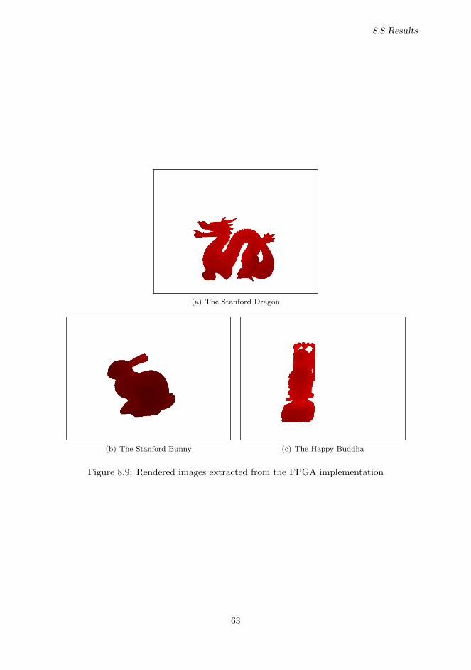
8.8 Results
(a) The Stanford Dragon
(b) The Stanford Bunny (c) The Happy Buddha
Figure 8.9: Rendered images extracted from the FPGA implementation
63

Chapter 8 Hardware Implementation
8.9 Discussion
The test results show that with a direct mapped cache, greater block size does not in factimprove rendering speed, even with large cache sizes (Table 8.2A). The small improve-ments seen with larger cache sizes in the software model is not apparent here. This canprobably be attributed to inaccuracies in the software cache model. It does appear thata 16 word block size is slightly better than an 8 word block size, and one can speculateif even larger block sizes would improve performance further. It is possible that the twoway set associative cache would have benefited from larger cache block sizes, but as thethe way set associative cache was implemented late in the thesis work, this has not beenexplored.
The relationships between the stack size and the cache size (Table 8.2B) show that largerstack sizes improve the performance of the design even when the cache size is large. Withboth no cache and a 512 word cache, the design is almost twice as fast with a 8 level cachecompared to no cache. There is no benefit to have a 16 level cache compared to 8 levels,which is not surprising as the octree is only 10 levels deep. There is a low probabilitythat a restart will be necessary when the stack is almost as deep as the octree, and if arestart does occur it is relatively cheap.
Table 8.2C shows that increasing stack size and core counts seems to improve performancemostly independently when in the presence of a small cache. However, the jump from 3to 4 cores seems to provide no performance benefit. In some instances it even decreasesperformance, but this difference is so small that no conclusions can be drawn from it.It is probably due to random variations in the rendering speed. The reason why morecores do not necessarily lead to better performance is probably due to congestion on thememory bus. When the memory bus is saturated the cores spend most their time waitingfor access to the memory bus.
The same congestion issues can be observed in Table 8.2D, where cache size and corecount is contrasted. These results illustrate that the larger the cache – the more coresthe memory bus can support. With no cache, adding extra cores does not improveperformance. With a cache, adding a second core improves rendering speed significantly.Although adding cores does seem to add some improvement for larger cache sizes, themost dramatic improvement is from 1 to 2 cores.
The same test of cache size vs. core count was done using a two way set associative cache(Table 8.2E). The results indicate a significant improvement across all configurations.This cache seems to improve utilization of the cores without increasing the cache size.This table also shows the design that achieved the best performance in the tests that wereperformed: a design with 4 cores, 1024 word cache, 1 word cache block size and a two wayset associative cache. Larger cache size were not tested due to issues with synthesizing.
Table 8.3 provides some interesting data on the resource use of the different design pa-rameters. For instance, the first two rows illustrate that a two way set associative cacherequires more LUTs but fewer LUT-RAMs. The reason is probably that the set asso-ciative cache requires an extra comparison unit and some extra logic. On the Spartan-6FPGA the LUT-RAMs seem to be interchangeable with LUTs, so the version with a twoway set associative cache wins on that measure. But it also requires more registers. In
64

8.9 Discussion
essence, the resource use is very similar between these designs. However, it is possiblethat the benefit of a two way set associative cache increases as the cache size increases,since the overhead of the two way set associative cache should be somewhat constant.
Looking at the design with a small stack size, it seems clear that it is better to have alarge stack size and a smaller cache, than a small stack and a larger cache. It is also clearthat among those designs the jump from 2 to 3 cores is not economical.
If we assume the design can achieve real time speed with a 640 x 480 image, by improvingthe scheduler and the cache system further, then we can try to estimate whether the designshould allow real time speeds at higher resolutions when implemented with state of theart integrated circuit technology. A commercial system should be able to render a fullHD image at a resolution of 1920 x 1080 pixels, which would imply that we need to traceat least 2 million pixels per frame. As we have seen, memory bandwidth is the criticalbottleneck in the design, and it is not unreasonable to assume that the performance scalessomewhat linearly with the memory bandwidth. A state of the art GPU has more than2 000 times more memory bandwidth than our system[61], which could potentially allowus to trace 2 billion rays per second, or 84 million rays per frame at 24 frames per second.This gives us 42 rays per pixel with full HD resolution, which should be enough for a widerange of effects, e.g., multiple light sources, reflections, ambient lighting and anti-aliasing.
To achieve this throughput the number of cores would probably also have to be increased,but it is difficult to evaluate how many cores could be included on a modern GPU. TheNVIDIA GeForce GTX 680 GPU contains 1536 CUDA cores[33], which are more capablethan the ray tracing cores presented in this thesis. A similar anecdote, is that Laineand Karras [29] achieved 24-170 million rays per second on a modern GPU by usingsoftware running on the CUDA cores. If the ray tracing cores are significantly smallerthan the CUDA cores, and can perform the ray tracing algorithm faster, then that is alsoan indication that a GPU could conceivably integrate enough cores to achieve real timespeed for high resolutions within a reasonable area.
There are many other factors that could affect this estimate. The GPU will probablyrequire much of the memory bandwidth to load color/texture data. In addition, somegames run at 60 frames per second. However, smarter caching and other optimizationscould allow the design to be even faster without increasing bandwidth requirements.Furthermore, the SVO model that was rendered in this thesis was only 10 levels deep,but if a game is to use the technique to render a vast landscape, it could require an SVOwhich is much deeper, and the performance impact of rendering a larger SVO has notbeen analyzed.
65

Chapter 8 Hardware Implementation
66

Chapter 9
Conclusions
In this thesis the outline of a practical design for ray tracing of sparse voxel octree inhardware has been presented. The final system approaches real-time speeds at a lowclock frequency, and with further work it is possible that this milestone could be passedwithout increasing the clock frequency. There is much work left before the design is acomplete and optimal system for ray tracing of SVOs in hardware. There are also manyunknown factors that affect the performance should the design be integrated in a modernGPU. However, the results shows that the technique is promising.
We have seen the value of maintaining a software version of the algorithm to aid in thedesign of a hardware implementation. It generated input data, implemented parts of thealgorithm which had not been done in hardware yet, was used to debug simulations of thehardware and provided data which could inform the choice of design parameters. Mostimportantly the software version demonstrated that rasterization and ray tracing couldpotentially be integrated in a hybrid rendering system, which would be essential in acommercially viable design.
The use of the ORPSoC system has shown the utility of open source in hardware design.It provided a complete and functional system for the chosen FPGA prototype board,which greatly simplified the process of creating a ray tracing system. The OpenRISCCPU proved very valuable in debugging the design, and adjusting the functionality ofthe system on the fly. In addition, the open source FPGALink software/firmware allowedfor easy and efficient communication with the board. The verilog simulator was opensource as well. In conclusion, almost all the intellectual property used in this thesis wascommunity created open source software and hardware. An added benefit of this wasthat most of the tools used was cross-platform, allowing development on any of the threebig operating systems. Only the commercial Xilinx synthesis tools were limited to justWindows and Linux.
The work on hardware optimizations have shown that the algorithm explored in thisthesis can be optimized in ways that are quite specific to hardware. By doing a carefulevaluation of the information required to implement the stack for the algorithm, we candrastically reduce the number of bits required for each level of the stack. The results
67

Chapter 9 Conclusions
from the hardware design testing shows the importance of evaluating the impact of designparameters. Using a stack which is at least half the size of the octree is one of the mosteconomical ways of boosting performance. Using a data cache is essential to improvingperformance, both by improving the speed of a single core, and to support more coresusing the same memory bus. Finally, using a two way set associative cache improves theutilization of the cores without increasing cache size.
The future of ray tracing in hardware is still uncertain. First, there is the question ofwhether one should implement ray tracing of polygon models, as demonstrated by Woopet al. [64], rather than using sparse voxel octrees. It is also conceivable that one couldconstruct a system which was flexible enough to do both. Second, it is possible that thesoftware implementations on GPGPUs, such as that of Laine and Karras [29], will befast enough on future GPGPUs, and that a dedicated hardware solution will be deemedtoo inflexible. There are many open questions, and more work is needed before we canconclude whether ray tracing in hardware is truly practical or not.
9.1 Future Work
We have not looked thoroughly at the possible data structures for sparse voxel octrees.As indicated by the experiments, memory bandwidth is crucial to performance, and amore efficient data structure could reduce the impact on bandwidth. The challenge is tocreate a data structure which can efficiently compress the SVO, while being fast enoughto decode in hardware without excessive resources. The data structure would have toincorporate and compress color data as well.
A large scale system for ray tracing of SVOs should also support streaming of voxel datafrom primary storage, as was demonstrated in software by Crassin et al. [10]. To use SVOsto model a large terrain could require tens of gigabytes if not more, and it is unreasonableto expect to hold all the data in memory at once. Enabling streaming of voxel data willpresent additional design challenges in both the design of the hardware and the datastructure.
There is currently very little research on the animation and deformation of SVOs[5].Animation of SVOs could increase the number of applications of the technique. To enablethis, one should perhaps look at accelerating the construction of SVOs in hardware aswell. If one could dynamically modify the SVOs in real time one could for instance createtire tracks in the dirt as a car drives across it. This is also something worth consideringwhen researching data structures for SVOs.
If these techniques are to be implemented in dedicated hardware on GPUs, one shouldtry to enable as many uses as possible to justify the cost. Octrees are a space partitioningstructure, and as mentioned in the chapter on space partitioning, these structures havemany uses in computer games. It could be wise to attempt to design the ray traversalmodule in a way that enables other uses.
It is clear that the design of the caches for the ray tracing cores has a very large impacton performance. Introducing cache hierarchies could further improve performance. Onecould introduce a small private cache to each core, have a set of cores share a larger
68

9.1 Future Work
cache, and have several sets of cores share an even larger one. The interplay betweenthe scheduler and the cache is also interesting. One could investigate a scheduler whichstarts a set of cores at the exact same time. If the cores are tracing coherent rays theyshould access some of the same node data at the same time, which could enable additionaloptimizations. Finally, there could yet be smart optimizations to the cache which couldexploit the specific memory access patterns of the ray tracing cores. There is still muchresearch that could be done on this subject.
69

Bibliography
[1] IEEE Standard for Floating-Point Arithmetic (754-2008), 2008.
[2] Alfred V Aho, Ravi Sethi, and Jeffrey D Ullman. Compilers: Principles,Techniques, and Tools. Addison Wesley, us ed edition, January 1986.
[3] Tomas Akenine-Moller, Eric Haines, and Naty Hoffman. Real-Time Ren-dering, Third Edition. AK Peters, 3 edition, July 2008.
[4] Mohit Arora. The Art of Hardware Architecture: Design Methods and Techniquesfor Digital Circuits. Springer, 2012 edition, October 2011.
[5] Dennis Bautembach. Animated Sparse Voxel Octrees, 2011. URL http://
bautembach.de/wordpress/wp-content/uploads/asvo.pdf. Retrieved on 2012-06-17.
[6] David Benson, Joel Davis, David Benson, and Joel Davis. Octree textures.In SIGGRAPH ’02 Proceedings of the 29th annual conference on Computer graphicsand interactive techniques, pages 785–790, New York, USA, July 2002. ACM.
[7] J Bittner, V Havran, and P Slavik. Hierarchical Visibility Culling with Oc-clusion Trees. In Computer Graphics International, pages 207–219. IEEE Comput.Soc, 1998.
[8] Mario Botsch, Andreas Wiratanaya, and Leif Kobbelt. Efficient high qual-ity rendering of point sampled geometry. Eurographics Association, July 2002.
[9] Per Christensen, Julian Fong, David Laur, and Dana Batali. Ray Tracingfor the Movie ‘Cars’. In 2006 IEEE Symposium on Interactive Ray Tracing, pages1–6. IEEE, 2006.
[10] Cyril Crassin, Fabrice Neyret, Sylvain Lefebvre, and Elmar Eisemann.Gigavoxels: Ray-Guided Streaming for Efficient and Detailed Voxel Rendering. InProceedings of the 2009 symposium on Interactive 3D graphics and games, pages15–22, New York, NY, USA, January 2009.
[11] Digilent Inc. Atlys Booard Reference Manual, 2011. URL http://digilent.us/
Data/Products/ATLYS/Atlys_rm.pdf. Retrieved on 2011-12-16.
[12] Daniel D Gajski, Nikil D Dutt, Allen C-H Wu, and Steve Y-L Lin. High-Level Synthesis: Introduction to Chip and System Design. Springer, 1st edition,February 1992.
70
BIBLIOGRAPHY
[13] H Ghasemzadeh, S Mazrouee, and M R Kakoee. Modified pseudo LRU re-placement algorithm. In 13th Annual IEEE International Symposium and Workshopon Engineering of Computer-Based Systems (ECBS’06), pages 6 pp.–376. IEEE,2006.
[14] Andrew S Glassner. An introduction to ray tracing. Academic Press, 1989.
[15] Enrico Gobbetti, Fabio Marton, and Jose Antonio Iglesias Guitian. Asingle-pass GPU ray casting framework for interactive out-of-core rendering of mas-sive volumetric datasets. The Visual Computer, 24(7-9):797–806, 2008.
[16] Eric Haines and Qingnan Zhou. binvox 3D mesh voxelizer, 2012. URL http:
//www.cs.princeton.edu/~min/binvox/. Retrieved on 2012-05-22.
[17] John L Hennessy and David A Patterson. Memory Hierarchy Design. In Com-puter Architecture: A Quantitative Approach, 4th Edition, pages 288–342. MorganKaufmann, September 2006.
[18] Charles Hollemeersch, Bart Pieters, Peter Lambert, and Rik Van deWalle. Accelerating virtual texturing using CUDA. In GPU Technology Conference,2009.
[19] Charles-Frederik Hollemeersch, Bart Pieters, Aljosha Demeule-meester, Frederik Cornillie, Bert Van Semmertier, Erik Mannens, Pe-ter Lambert, Piet Desmet, and Rik Van de Walle. Infinitex: An interactiveediting system for the production of large texture data sets. Computers &Graphics, 34(6):643–654, December 2010.
[20] H Hoppe. Smooth view-dependent level-of-detail control and its application toterrain rendering. In Visualization ’98, pages 35–42,. IEEE, 1998.
[21] Daniel Reiter Horn, Jeremy Sugerman, Mike Houston, and Pat Hanra-han. Interactive kd tree GPU raytracing. In Symposium on Interactive 3D Graphicsand Games, Seattle, Washington, 2007.
[22] Fumihiko Ino, Jun Gomita, Yasuhiro Kawasaki, and Kenichi Hagihara. AGPGPU Approach for Accelerating 2-D/3-D Rigid Registration of Medical Images. InMinyi Guo, Laurence Yang, Beniamino Di Martino, Hans Zima, Jack Dongarra, andFeilong Tang, editors, Parallel and Distributed Processing and Applications, pages939–950. Springer Berlin / Heidelberg, Berlin, Heidelberg, 2006.
[23] Arie Kaufman. Volume visualization. The Visual Computer, 6(1):1–1, January1990.
[24] Shoab Ahmed Khan. Digital Design of Signal Processing Systems: A PracticalApproach. Wiley, 1 edition, February 2011.
[25] Aaron M Knoll, Ingo Wald, and Charles D Hansen. Coherent multiresolu-tion isosurface ray tracing. The Visual Computer, 25(3):209–225, March 2008.
[26] Isreal Koren. Computer arithmetic algorithms. Ak Peters Series. A K Peters,2002.
71

BIBLIOGRAPHY
[27] Stefan Kristiansson. ORPSoC on Digilent Atlys, 2012. URL http://www.
chokladfabriken.org/projects/orpsoc-atlys. Retrieved on 2012-06-16.
[28] Ian Kuon, Russell Tessier, and Jonathan Rose. FPGA Architecture: Surveyand Challenges. Foundations and Trends R© in Electronic Design Automation, 2(2):135–253, 2007.
[29] Samuli Laine and Tero Karras. Efficient Sparse Voxel Octrees. Symposium onInteractive 3D Graphics and Games, February 2010.
[30] Samuli Laine and Tero Karras. Efficient Sparse Voxel Octrees – Analysis,Extensions, and Implementation, February 2010. URL http://code.google.com/
p/efficient-sparse-voxel-octrees/.
[31] Marc Levoy. Efficient ray tracing of volume data. ACM Transactions on Graphics,9(3):245–261, July 1990.
[32] Chris McClelland. FPGALink, 2011. URL http://www.makestuff.eu/
wordpress/?page_id=1400. Retrieved on 2011-12-15.
[33] NVIDIA Corporation. Nvidia geforce gtx 680, 2012. URL http://www.geforce.
com/Active/en_US/en_US/pdf/GeForce-GTX-680-Whitepaper-FINAL.pdf. Re-trieved on 20212-06-16.
[34] NVIDIA Corporation. High Performance Computing, 2012. URL http://www.
nvidia.com/object/tesla-supercomputing-solutions.html. Retrieved on 2012-05-18.
[35] OpenCores. Wishbone B4 - Wishbone System-on-chip (SoC) Interconnection Ar-chitecture for Portable IP Cores. OpenCores, 2011. URL http://opencores.org/
opencores,wishbone. Retrieved on 2011-12-15.
[36] OpenCores. OpenRISC 1200 IP Core Specification (Preliminary Draft). Open-Cores, 2012. URL http://opencores.org/openrisc,or1200. Retrieved on 2012-06-15.
[37] Sudeep Pasricha and Nikil Dutt. On-Chip Communication Architectures: Sys-tem on Chip Interconnect (Systems on Silicon). Morgan Kaufmann, 1 edition, May2008.
[38] Jingliang Peng, C.-C. Jay Kuo, Jingliang Peng, and C.-C. Jay Kuo.Geometry-guided progressive lossless 3D mesh coding with octree (OT) decompo-sition. ACM Transactions on Graphics (TOG), 24(3):609–616, July 2005.
[39] Naila Rahman. Algorithms for Hardware Caches and TLB. In Ulrich Meyer, PeterSanders, and Jop Sibeyn, editors, Lecture Notes in Computer Science, pages 171–192.Springer Berlin Heidelberg, Berlin, Heidelberg, February 2003.
[40] S. Raje and R. A. Bergamaschi. Generalized resource sharing. IEEE ComputerSociety, November 1997.
[41] J. Revelles, C. Urena, and M. Lastra. An Efficient Parametric Algorithm forOctree Traversal. Journal of WSCG, pages 212–219, January 2000.
72

BIBLIOGRAPHY
[42] Kristof Romisch. Sparse voxel octree ray tracing on the GPU. Master’s thesis,Aarhus University, 2009.
[43] Jorg Schmittler, Sven Woop, Daniel Wagner, Wolfgang J. Paul, andPhilipp Slusallek. Realtime Ray Tracing of Dynamic Scenes on an FPGA Chip.In Proceedings of the ACM SIGGRAPH/EUROGRAPHICS conference on Graphicshardware, page 95, New York, New York, USA, 2004. ACM Press.
[44] Jorg Schmittler, Daniel Pohl, Tim Dahmen, Christian Vogelgesang,and Philipp Slusallek. Realtime ray tracing for current and future games. InACM SIGGRAPH 2005 Courses, page 23, New York, New York, USA, 2005. ACMPress.
[45] Ruwen Schnabel and Reinhard Klein. Octree-based Point-Cloud Compression.In Eurographics Symposium on Point-Based Graphics (2006). Institut fur InformatikII, Universitat Bonn, Germany, 2006.
[46] D Sheldon, R Kumar, F Vahid, D Tullsen, and R Lysecky. Conjoining Soft-Core FPGA Processors. In Computer-Aided Design, 2006. ICCAD ’06. IEEE/ACMInternational Conference on, pages 694–701, 2006.
[47] Ryan Shrout. John Carmack on id Tech 6, Ray Tracing, Consoles, Physicsand more, 2008. URL http://www.pcper.com/reviews/Graphics-Cards/
John-Carmack-id-Tech-6-Ray-Tracing-Consoles-Physics-and-more. Re-trieved on 2012-06-15.
[48] Ryan Shrout. John Carmack Interview: GPU Race, Intel Graphics, Ray Trac-ing, Voxels and more!, 2011. URL http://www.pcper.com/reviews/Editorial/
John-Carmack-Interview-GPU-Race-Intel-Graphics-Ray-Tracing-Voxels-and-more.Retrieved on 2012-06-15.
[49] John Spackman and Philip Willis. The SMART navigation of a ray through anoct-tree. Computers & graphics, 15(2):185–194, 1991.
[50] Stanford Computer Graphics Laboratory. Scanning and surface reconstruc-tion, 2012. URL http://graphics.stanford.edu/data/3Dscanrep/. Retrieved on2012-05-22.
[51] Nilo Stolte and Rene Caubet. Discrete Ray-Tracing of Huge Voxel Spaces.Computer Graphics Forum, 14(3):383–394, August 1995.
[52] K R Subramanian and D S Fussell. Applying Space Subdivision Techniques toVolume Rendering. In First IEEE Conference on Visualization: Visualization ‘90,pages 150–159,. IEEE Comput. Soc. Press, 1990.
[53] TSB Sudarshan and RA Mir. Highly efficient LRU implementations for highassociativity cache memory. In Proceedings of 12th . . . , 2004.
[54] Kelvin Sung. A DDA Octree Traversal Algorithm for Ray Tracing. In EurographicsConference Proceedings 1991, 1991.
[55] L Szirmay-Kalos, V Havran, and B Balazs. On the efficiency of ray-shootingacceleration schemes. In Proceedings of the 18th . . . , 2002.
73

BIBLIOGRAPHY
[56] Branislav Sıles. Atomontage Engine - Home, 2012. URL http://www.
atomontage.com/. Retrieved on 2012-05-18.
[57] JMP Van Waveren. Van Waveren: id Tech 5 Challenges-From Texture Virtualiza...- Google Scholar. In SIGGRAPH 2009: . . . , 2009.
[58] Kyu-Young Whang, Ju-Won Song, Ji-Woong Chang, Ji-Yun Kim, Wan-Sup Cho, Chong-Mok Park, and Il-Yeol Song. Octree-R: an adaptive octreefor efficient ray tracing. IEEE Transactions on Visualization and Computer Graphics,1(4):343–349, 1995.
[59] Wikipedia. Rasterization. URL http://en.wikipedia.org/wiki/Rasterisation.Retrieved on 2012-06-17.
[60] Wikipedia. Geforce 500 series, 2012. URL http://en.wikipedia.org/wiki/
GeForce_500_Series. Retrieved on 2012-03-22.
[61] Wikipedia. Geforce 600 series, 2012. URL http://en.wikipedia.org/wiki/
GeForce_600_Series. Retrieved on 2012-06-16.
[62] Wikipedia. Nvidia tesla, 2012. URL http://en.wikipedia.org/wiki/Nvidia_
Tesla. Retrieved on 2012-05-18.
[63] Wayne Wolf. Computers as Components, Second Edition: Principles of EmbeddedComputing System Design. Morgan Kaufmann, 2 edition, June 2008.
[64] Sven Woop, Jorg Schmittler, and Philipp Slusallek. RPU: A Pro-grammable Ray Processing Unit for Realtime Ray Tracing. ACM SIGGRAPH 2005Papers, pages 434–444, April 2005.
[65] Xilinx Inc. LogiCORE IP Adder/Subtracter v11., 2011. URL http://www.xilinx.
com/support/documentation/ip_documentation/addsub_ds214.pdf. Retrievedon 2012-03-22.
[66] Xilinx Inc. LogiCORE IP Floating-Point Operator v5.0, 2011. URLhttp://www.xilinx.com/support/documentation/ip_documentation/
floating_point_ds335.pdf. Retrieved on 2012-03-22.
[67] Xilinx Inc. LogiCORE IP Multiplier v11.2, 2011. URL http://www.xilinx.com/
support/documentation/ip_documentation/mult_gen_ds255.pdf. Retrieved on2012-03-22.
[68] Xilinx Inc. Spartan-6 Family Overview, 2011. URL http://www.xilinx.com/
support/documentation/data_sheets/ds160.pdf. Retrieved on 2011-12-16.
74

Appendix A
Attached Files
raycaster/ -- The Verilog source of the ray caster module
raycast_core_axis_dp.v -- The datapath of the per-axis calculations
raycast_core_idx.v -- The datapath of the index calculations
raycast_core_master.v -- The memory request unit of the core
raycast_core.v -- The ray casting core
raycast_ctrl.v -- The scheduler / control unit
raycast_master.v -- The ray caster memory interface / cache
raycast_slave.v -- The slave interface
raycaster.v -- The ray caster top level module
oppgave.pdf -- This report
orpsoc/ -- HDL, Software and Makefiles for the full ORPSoC-based system
sim/ -- The bench for simulation of the hardware module
out/ -- The source and synthesis output of the designs
data/ -- The octree and ray data used to test the designs
Octree2/ -- The software application
orlink/
hw/ -- HDL code and Sim. bench for orlink
sw/ -- CLI software to communicate with orlink
75

Appendix B
The Software Ray TracingCore Functions
RayCastOutput rayCast(Ray r)
{
Ray r2 = r;
int dir_mask=0;
// if (fabs(r.o.x)>o_max ||
// fabs(r.o.y)>o_max ||
// fabs(r.o.z)>o_max)
// throw;
if (r.d.x==0)
r.d.x+=0.001;
if (r.d.x<0.0) {
r.o.x = -r.o.x;
r.d.x = -r.d.x;
dir_mask |= 4;
}
if (r.d.y==0)
r.d.y+=0.001;
if (r.d.y<0.0) {
r.o.y = -r.o.y;
r.d.y = -r.d.y;
dir_mask |= 2;
}
if (r.d.z==0)
r.d.z+=0.001;
if (r.d.z<0.0) {
r.o.z = -r.o.z;
r.d.z = -r.d.z;
dir_mask |= 1;
}
float tx0, tx1, ty0, ty1, tz0, tz1;
tx0 = (-1-r.o.x)/r.d.x;
tx1 = (1-r.o.x)/r.d.x;
76
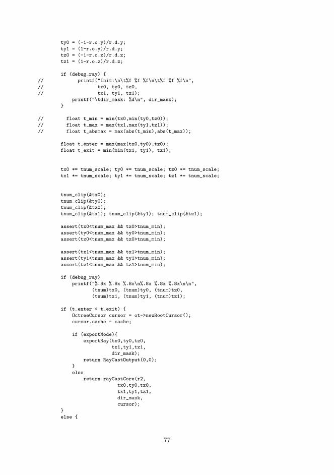
ty0 = (-1-r.o.y)/r.d.y;
ty1 = (1-r.o.y)/r.d.y;
tz0 = (-1-r.o.z)/r.d.z;
tz1 = (1-r.o.z)/r.d.z;
if (debug_ray) {
// printf("Init:\n\t%f %f %f\n\t%f %f %f\n",
// tx0, ty0, tz0,
// tx1, ty1, tz1);
printf("\tdir_mask: %d\n", dir_mask);
}
// float t_min = min(tx0,min(ty0,tz0));
// float t_max = max(tx1,max(ty1,tz1));
// float t_absmax = max(abs(t_min),abs(t_max));
float t_enter = max(max(tx0,ty0),tz0);
float t_exit = min(min(tx1, ty1), tz1);
tx0 *= tnum_scale; ty0 *= tnum_scale; tz0 *= tnum_scale;
tx1 *= tnum_scale; ty1 *= tnum_scale; tz1 *= tnum_scale;
tnum_clip(&tx0);
tnum_clip(&ty0);
tnum_clip(&tz0);
tnum_clip(&tx1); tnum_clip(&ty1); tnum_clip(&tz1);
assert(tx0<tnum_max && tx0>tnum_min);
assert(ty0<tnum_max && ty0>tnum_min);
assert(tz0<tnum_max && tz0>tnum_min);
assert(tx1<tnum_max && tx1>tnum_min);
assert(ty1<tnum_max && ty1>tnum_min);
assert(tz1<tnum_max && tz1>tnum_min);
if (debug_ray)
printf("%.8x %.8x %.8x\n%.8x %.8x %.8x\n\n",
(tnum)tx0, (tnum)ty0, (tnum)tz0,
(tnum)tx1, (tnum)ty1, (tnum)tz1);
if (t_enter < t_exit) {
OctreeCursor cursor = ot->newRootCursor();
cursor.cache = cache;
if (exportMode){
exportRay(tx0,ty0,tz0,
tx1,ty1,tz1,
dir_mask);
return RayCastOutput(0,0);
}
else
return rayCastCore(r2,
tx0,ty0,tz0,
tx1,ty1,tz1,
dir_mask,
cursor);
}
else {
77

Chapter B The Software Ray Tracing Core Functions
if (exportMode)
exportRay(0,0,0,0,0,0, (1<<31));
}
if (debug_ray) printf("End.\n");
return RayCastOutput(0,false);
}
RayCastOutput rayCastCore(Ray ray,
tnum r_tx0, tnum r_ty0, tnum r_tz0,
tnum r_tx1, tnum r_ty1, tnum r_tz1,
int dir_mask,
OctreeCursor r_cur)
{
int level;
int idx, idx_flip;
bool is_first_node;
bool exits_node;
bool pass_node;
tnum t_start = 0;
tnum t_enter;
tnum t_exit_child;
tnum tx0, ty0, tz0;
tnum tx1, ty1, tz1;
tnum txm, tym, tzm;
tnum tx0_child, ty0_child, tz0_child;
tnum tx1_child, ty1_child, tz1_child;
bool is_leaf;
tnum t_out;
OctreeCursor cur;
S_INIT:
cur = r_cur;
tx0 = r_tx0; ty0 = r_ty0; tz0 = r_tz0;
tx1 = r_tx1; ty1 = r_ty1; tz1 = r_tz1;
is_first_node = true;
level = 0;
exits_node = false;
stack->reset();
if (debug_ray)
printf("Init - t_start: %.8x\n", t_start);
goto S_CALC_T;
S_CALC_T:
txm = (tx0+tx1)/2;
tym = (ty0+ty1)/2;
tzm = (tz0+tz1)/2;
t_enter = max(tx0,max(ty0,tz0));
78

if (debug_ray)
printf("t_enter: %.8x\n", t_enter);
if (is_first_node)
goto S_FIRST_IDX;
else
goto S_NEXT_IDX;
S_FIRST_IDX:
idx = (txm < t_enter)<<2 | (tym < t_enter)<<1 | (tzm < t_enter);
exits_node = false;
is_first_node = false;
if (debug_ray)
printf("FrstIdx: %d / %d\n", idx, idx^dir_mask);
goto S_DATA_WAIT;
S_DATA_WAIT:
// if (got_data)
if (debug_ray)
printf("Data: %.8x : %.8x\n", cur.adr*4, *((int*)cur.node));
goto S_CALC_CHILD_T;
S_NEXT_IDX:
exits_node = false;
if (t_exit_child == tx1_child) {
if (idx & 4)
exits_node = true;
else
idx = idx ^ 4;
}
else if (t_exit_child == ty1_child) {
if (idx & 2)
exits_node = true;
else
idx = idx ^ 2;
}
else {
if (idx & 1)
exits_node = true;
else
idx = idx ^ 1;
}
if (debug_ray)
printf("NextIdx: %d / %d exit: %d\n", idx, idx^dir_mask, exits_node);
goto S_NEXT_EVAL;
S_NEXT_EVAL:
if (exits_node) {
if (level==0) {
is_leaf = false;
goto S_FINISHED;
}
else if (stack->empty()) {
if (debug_ray)
printf("Underflow\n\n");
restart_count++;
t_start = t_exit_child;
79

Chapter B The Software Ray Tracing Core Functions
goto S_INIT;
}
else {
if (debug_ray) printf("Pop\n");
stack->pop(&cur,
&tx0, &ty0, &tz0,
&tx1, &ty1, &tz1,
&idx);
level--;
goto S_CALC_T;
}
}
else {
goto S_CALC_CHILD_T;
}
S_CALC_CHILD_T:
// if (debug_ray) printf("Idx %d / %d\n", idx, idx ^ dir_mask);
tx0_child = (idx&4) ? txm : tx0;
tx1_child = (idx&4) ? tx1 : txm;
ty0_child = (idx&2) ? tym : ty0;
ty1_child = (idx&2) ? ty1 : tym;
tz0_child = (idx&1) ? tzm : tz0;
tz1_child = (idx&1) ? tz1 : tzm;
t_exit_child = min(tx1_child,min(ty1_child,tz1_child));
goto S_EVAL;
S_EVAL:
idx_flip = idx ^ dir_mask;
pass_node = t_exit_child <= t_start;
if (pass_node) {
goto S_NEXT_IDX;
}
else if (cur.childIsFilled(idx_flip) || level==terminLevel) {
tx0 = tx0_child; ty0 = ty0_child; tz0 = tz0_child;
tx1 = tx1_child; ty1 = ty1_child; tz1 = tz1_child;
is_leaf = true;
goto S_FINISHED;
}
else if (cur.childIsValid(idx_flip)) {
if (debug_ray) {
// printf("%.8x %.8x %.8x\n%.8x %.8x %.8x\n",
// tx0, ty0, tz0, tx1, ty1, tz1);
if (cur.childPtrIsFar())
printf("Far %x\n", cur.farPtr());
printf("Push\n\n");
}
if (cur.childPtrIsFar()) {
far_count++;
}
push_count++;
stack->push(cur,
tx0, ty0, tz0,
tx1, ty1, tz1,
idx);
tx0 = tx0_child; ty0 = ty0_child; tz0 = tz0_child;
tx1 = tx1_child; ty1 = ty1_child; tz1 = tz1_child;
80

level++;
is_first_node = true;
cur = cur.getChild(idx_flip);
goto S_CALC_T;
}
else {
goto S_NEXT_IDX;
}
S_FINISHED:
t_enter = max(tx0,max(ty0,tz0));
t_out = is_leaf ? t_enter : t_exit_child;
if (debug_ray) {
printf("Leaf: %d %.8x\n\n\n", is_leaf, t_out);
}
return RayCastOutput((float)t_out/(float)tnum_scale, is_leaf);
}
81

Appendix C
The Ray Tracing Core Module
// TODO: Implement error when level overflows
‘include "raycast_defines.v"
module raycast_core
(
clk, rst,
start_i,
root_adr_i,
dir_mask_i,
tx0_i, ty0_i, tz0_i,
tx1_i, ty1_i, tz1_i,
m_wb_adr_o, m_wb_dat_i,
m_wb_cyc_o, m_wb_stb_o,
m_wb_ack_i,
finished_o, leaf_o, t_o, level_o
);
// = Parameters =
parameter dw = 32; // Data width
parameter stack_size = 8;
parameter stack_size_log2 = 3;
parameter max_lvl = 32;
parameter max_lvl_log2 = 5;
// --
// = Ports =
input clk;
input rst;
input start_i;
input [31:0] root_adr_i;
input [2:0] dir_mask_i;
input [dw-1:0] tx0_i, ty0_i, tz0_i;
82

input [dw-1:0] tx1_i, ty1_i, tz1_i;
// WISHBONE master
output [31:0] m_wb_adr_o;
input [31:0] m_wb_dat_i;
output m_wb_cyc_o;
output m_wb_stb_o;
input m_wb_ack_i;
output reg finished_o; reg finished_o_n;
output reg leaf_o; reg leaf_o_n;
output [dw-1:0] t_o;
output [max_lvl_log2-1:0] level_o;
// --
// = States =
parameter S_IDLE = 0, S_INIT = 1,
S_CALC_T = 2, S_FIRST_IDX = 3,
S_NEXT_EVAL = 4, S_CALC_CHILD_T = 5, S_EVAL = 6, S_FINISHED = 7;
// --
parameter EXIT_X = 2’b01, EXIT_Y = 2’b10, EXIT_Z = 2’b00;
// = Registers/Memories =
reg [31:0] root_adr, root_adr_n;
reg [2:0] dir_mask, dir_mask_n;
reg signed [dw-1:0] tx0_root, tx0_root_n;
reg signed [dw-1:0] ty0_root, ty0_root_n;
reg signed [dw-1:0] tz0_root, tz0_root_n;
reg signed [dw-1:0] tx1_root, tx1_root_n;
reg signed [dw-1:0] ty1_root, ty1_root_n;
reg signed [dw-1:0] tz1_root, tz1_root_n;
reg [2:0] state, state_n;
reg [max_lvl_log2-1:0] level;
reg [1:0] expl_child, expl_child_n; // Child exit plane
reg signed [dw-1:0] t_exit_child, t_exit_child_n;
reg signed [dw-1:0] t_enter, t_enter_n;
reg signed [dw-1:0] t_start, t_start_n;
reg [2:0] idx, idx_n;
reg [2:0] idx_prev, idx_prev_n;
reg is_first_node, is_first_node_n;
// --
// = Wires/Aliases =
wire signed [dw-1:0] tx0;
wire signed [dw-1:0] ty0;
wire signed [dw-1:0] tz0;
wire signed [dw-1:0] txm;
wire signed [dw-1:0] tym;
wire signed [dw-1:0] tzm;
wire signed [dw-1:0] tx1;
83
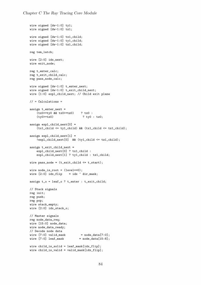
Chapter C The Ray Tracing Core Module
wire signed [dw-1:0] ty1;
wire signed [dw-1:0] tz1;
wire signed [dw-1:0] tx1_child;
wire signed [dw-1:0] ty1_child;
wire signed [dw-1:0] tz1_child;
reg tem_latch;
wire [2:0] idx_next;
wire exit_node;
reg t_enter_calc;
reg t_exit_child_calc;
reg pass_node_calc;
wire signed [dw-1:0] t_enter_next;
wire signed [dw-1:0] t_exit_child_next;
wire [1:0] expl_child_next; // Child exit plane
// = Calculations =
assign t_enter_next =
(tx0>=ty0 && tx0>=tz0) ? tx0 :
(ty0>=tz0) ? ty0 : tz0;
assign expl_child_next[0] =
(tx1_child <= ty1_child) && (tx1_child <= tz1_child);
assign expl_child_next[1] =
!expl_child_next[0] && (ty1_child <= tz1_child);
assign t_exit_child_next =
expl_child_next[0] ? tx1_child :
expl_child_next[1] ? ty1_child : tz1_child;
wire pass_node = (t_exit_child <= t_start);
wire node_is_root = (level==0);
wire [2:0] idx_flip = idx ^ dir_mask;
assign t_o = leaf_o ? t_enter : t_exit_child;
// Stack signals
reg init;
reg push;
reg pop;
wire stack_empty;
wire [2:0] idx_stack_o;
// Master signals
reg node_data_req;
wire [15:0] node_data;
wire node_data_ready;
// Decode node data
wire [7:0] valid_mask = node_data[7:0];
wire [7:0] leaf_mask = node_data[15:8];
wire child_is_solid = leaf_mask[idx_flip];
wire child_is_valid = valid_mask[idx_flip];
84

// --
// = Datapath Instances =
raycast_core_axis_dp x_axis_dp
(
.clk (clk),
.rst (rst),
.init_i (init),
.push_i (push),
.pop_i (pop),
.tem_latch_i (tem_latch),
.idx_i (idx[2]),
.idx_prev_i (idx_prev[2]),
.te0_i (tx0_root),
.te1_i (tx1_root),
.te0_o (tx0),
.tem_o (txm),
.te1_o (tx1),
.te1_child_o (tx1_child)
);
defparam x_axis_dp.dw = dw;
defparam x_axis_dp.stack_size = stack_size+1;
raycast_core_axis_dp y_axis_dp
(
.clk (clk),
.rst (rst),
.init_i (init),
.push_i (push),
.pop_i (pop),
.tem_latch_i (tem_latch),
.idx_i (idx[1]),
.idx_prev_i (idx_prev[1]),
.te0_i (ty0_root),
.te1_i (ty1_root),
.te0_o (ty0),
.tem_o (tym),
.te1_o (ty1),
.te1_child_o (ty1_child)
);
defparam y_axis_dp.dw = dw;
defparam y_axis_dp.stack_size = stack_size+1;
raycast_core_axis_dp z_axis_dp
(
.clk (clk),
.rst (rst),
.init_i (init),
.push_i (push),
.pop_i (pop),
.tem_latch_i (tem_latch),
.idx_i (idx[0]),
.idx_prev_i (idx_prev[0]),
.te0_i (tz0_root),
.te1_i (tz1_root),
.te0_o (tz0),
85

Chapter C The Ray Tracing Core Module
.tem_o (tzm),
.te1_o (tz1),
.te1_child_o (tz1_child)
);
defparam z_axis_dp.dw = dw;
defparam z_axis_dp.stack_size = stack_size+1;
raycast_core_idx idx_next_dp
(
.is_first_i (is_first_node),
.idx_i (idx),
.txm_i (txm),
.tym_i (tym),
.tzm_i (tzm),
.t_enter_i (t_enter),
.exit_plane_child_i (expl_child),
.idx_next_o(idx_next),
.is_exit_o(exit_node)
);
defparam idx_next_dp.dw = dw;
raycast_core_master core_master
(
.clk (clk),
.rst (rst),
.m_wb_adr_o (m_wb_adr_o),
.m_wb_dat_i (m_wb_dat_i),
.m_wb_cyc_o (m_wb_cyc_o),
.m_wb_stb_o (m_wb_stb_o),
.m_wb_ack_i (m_wb_ack_i),
.init_i (init),
.pop_i (pop),
.root_adr_i (root_adr),
.idx_flip_i (idx_flip),
.node_data_req_i (node_data_req),
.node_data_ready_o (node_data_ready),
.node_data_o (node_data)
);
defparam core_master.stack_size = stack_size;
defparam core_master.stack_size_log2 = stack_size_log2;
// --
// = Control FSM =
always @(*)
begin
root_adr_n = root_adr;
dir_mask_n = dir_mask;
tx0_root_n = tx0_root;
ty0_root_n = ty0_root;
tz0_root_n = tz0_root;
tx1_root_n = tx1_root;
ty1_root_n = ty1_root;
tz1_root_n = tz1_root;
state_n = state;
expl_child_n = expl_child;
86

t_exit_child_n = t_exit_child;
t_enter_n = t_enter;
t_start_n = t_start;
idx_prev_n = idx_prev;
idx_n = idx;
is_first_node_n = is_first_node;
leaf_o_n = leaf_o;
finished_o_n = finished_o;
t_enter_calc = 0;
t_exit_child_calc = 0;
pass_node_calc = 0;
tem_latch = 0;
init = 0;
push = 0;
pop = 0;
node_data_req = 0;
case (state)
S_IDLE: begin // 0
if (start_i) begin
root_adr_n = root_adr_i;
dir_mask_n = dir_mask_i;
tx0_root_n = tx0_i;
ty0_root_n = ty0_i;
tz0_root_n = tz0_i;
tx1_root_n = tx1_i;
ty1_root_n = ty1_i;
tz1_root_n = tz1_i;
t_start_n = 0;
finished_o_n = 0;
state_n = S_INIT;
end
end
S_INIT: begin // 1
// Fetch root data
// Set level = 0
// Reset stack
init = 1;
is_first_node_n = 1;
state_n = S_CALC_T;
end
S_CALC_T: begin // 2
// tm <= (t0+t1)/2 (in axis_dp)
tem_latch = 1;
// t_enter <= min(t0)
t_enter_calc = 1;
t_enter_n = t_enter_next;
if (is_first_node)
state_n = S_FIRST_IDX;
else
state_n = S_NEXT_EVAL;
end
S_FIRST_IDX: begin // 3
87
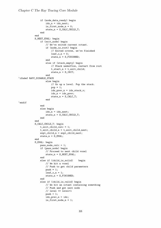
Chapter C The Ray Tracing Core Module
if (node_data_ready) begin
idx_n = idx_next;
is_first_node_n = 0;
state_n = S_CALC_CHILD_T;
end
end
S_NEXT_EVAL: begin
if (exit_node) begin
// We’ve exited current octant.
if (node_is_root) begin
// Exited octree, we’re finished
leaf_o_n = 0;
state_n = S_FINISHED;
end
else if (stack_empty) begin
// Stack underflow, restart from root
t_start_n = t_exit_child;
state_n = S_INIT;
end
‘ifndef RAYC_DISABLE_STACK
else begin
// Go up a level. Pop the stack.
pop = 1;
idx_prev_n = idx_stack_o;
idx_n = idx_prev;
state_n = S_CALC_T;
end
‘endif
end
else begin
idx_n = idx_next;
state_n = S_CALC_CHILD_T;
end
end
S_CALC_CHILD_T: begin
t_exit_child_calc = 1;
t_exit_child_n = t_exit_child_next;
expl_child_n = expl_child_next;
state_n = S_EVAL;
end
S_EVAL: begin
pass_node_calc = 1;
if (pass_node) begin
// Proceed to next child voxel
state_n = S_NEXT_EVAL;
end
else if (child_is_solid) begin
// We hit a voxel
// Push to get child parameters
push = 1;
leaf_o_n = 1;
state_n = S_FINISHED;
end
else if (child_is_valid) begin
// We hit an octant containing something
// Push and get next node
// level <= level+1
push = 1;
idx_prev_n = idx;
is_first_node_n = 1;
88

node_data_req = 1;
state_n = S_CALC_T;
end
else begin
// Empty octant, evaluate next child node
state_n = S_NEXT_EVAL;
end
end
S_FINISHED: begin
// Calculate t_enter for child
t_enter_calc = 1;
t_enter_n = t_enter_next;
finished_o_n = 1;
state_n = S_IDLE;
end
endcase
end
// --
// = Registers =
always @(posedge clk)
begin
if (rst) begin
root_adr <= 32’d0;
dir_mask <= 3’d0;
tx0_root <= 32’d0;
ty0_root <= 32’d0;
tz0_root <= 32’d0;
tx1_root <= 32’d0;
ty1_root <= 32’d0;
tz1_root <= 32’d0;
state <= 3’d0;
level <= 0;
expl_child <= 2’d0;
t_exit_child <= 32’d0;
t_enter <= 32’d0;
t_start <= 32’d0;
idx_prev <= 3’d0;
idx <= 3’d0;
is_first_node <= 0;
finished_o <= 1;
leaf_o <= 0;
end
else
begin
root_adr <= root_adr_n;
dir_mask <= dir_mask_n;
tx0_root <= tx0_root_n;
ty0_root <= ty0_root_n;
tz0_root <= tz0_root_n;
tx1_root <= tx1_root_n;
ty1_root <= ty1_root_n;
tz1_root <= tz1_root_n;
89

Chapter C The Ray Tracing Core Module
state <= state_n;
expl_child <= expl_child_n;
t_exit_child <= t_exit_child_n;
t_enter <= t_enter_n;
t_start <= t_start_n;
idx <= idx_n;
idx_prev <= idx_prev_n;
is_first_node <= is_first_node_n;
finished_o <= finished_o_n;
leaf_o <= leaf_o_n;
if (init)
level <= 0;
else if (push)
level <= level + 1;
else if (pop)
level <= level - 1;
else
level <= level;
end
end
// --
// = Stacks =
‘ifndef RAYC_DISABLE_STACK
reg [stack_size_log2:0] stack_depth;
wire stack_full = (stack_depth==stack_size);
assign stack_empty = (stack_depth==0);
always @(posedge clk)
if (init) begin
stack_depth <= 0;
end
else if (push) begin
if (!stack_full)
stack_depth <= stack_depth + 1;
end
else if (pop) begin
stack_depth <= stack_depth - 1;
end
raycast_stack idx_stack_inst
(
.clk (clk),
.push (push),
.pop (pop),
.data_i (idx_prev),
.data_o (idx_stack_o)
);
defparam idx_stack_inst.dw = 3;
defparam idx_stack_inst.depth = stack_size; ///-1
defparam idx_stack_inst.depth_log2 = stack_size_log2;
‘else
90

assign stack_empty = 1;
‘endif
// --
endmodule
91