Efficient Directional Network Backbone Construction inMobile Ad Hoc Networks

Shuhui Yang†, Jie Wu‡, and Fei Dai§†Department of Computer Science

Rensselaer Polytechnic InstituteTroy, NY 12180

†Department of Computer Science and EngineeringFlorida Atlantic University

Boca Raton, FL 33431§Microsoft Corporation

Seattle, WA 98104

Abstract

In this paper, we consider the issue of constructing an energy-efficient virtual network back-

bone in mobile ad hoc networks (MANETs) for broadcasting applications using directional an-

tennas. In directional antenna models, the transmission/reception range is divided into several

sectors, and one or more sectors can be switched on for transmission. Therefore, data forwarding

can be restricted to certain directions (sectors), and both energy consumption and interference can

be reduced. We develop the notation of our directional network backbone using the directional

antenna model, and form the problem of the directional connected dominating set (DCDS) which

is an extreme case of the directional network backbone using an unlimited number of directional

antennas. The minimum DCDS problem is proved to be NP-complete. A localized heuristic

algorithm for constructing a small DCDS and two extensions of the algorithm are proposed. Per-

formance analysis includes an analytical study in terms of an approximation ratio and a simulation

study on the proposed algorithms using both a custom simulator and ns2.

Keywords: Connected dominating set (CDS), directional antennas, local solution, mobile ad hoc

networks (MANETs), virtual network backbone.

1

1 Introduction

Broadcasting is the most frequently used operation in mobile ad hoc networks (MANETs) for the

dissemination of data and control messages in the preliminary stages of some other applications.

Usually, a wired network backbone is constructed for efficient broadcasting, where only selected

nodes that form the backbone forward data and the entire network receives it. The dominating set

(DS) has been widely used to select an efficient virtual network backbone. A set is dominating if

every node in the network is either in the set or a neighbor of a node in the set. When a DS is

connected, it is called a connected dominating set (CDS). In a CDS, any two nodes in the DS can be

connected through intermediate nodes from the DS. Using a CDS a a connected, virtual backbone has

been widely used for efficient broadcasting in MANETs. In [13] it is demonstrated that any broadcast

scheme based on a backbone with size proportional to the minimum CDS guarantees a throughput

within a constant factor of the broadcast capacity. CDS has been used in many other applications,

including sensor coverage [1] and efficient communication using network coding [15].

In a directed graph, the set in the virtual network backbone for broadcasting is called the connected

dominating and absorbent set [31]. If two nodes are connected by a directed edge, the start node is

a dominating neighbor of the end node, and the end node is an absorbent neighbor of the start node.

In a connected dominating and absorbent set, nodes in the set are strongly connected, and each node

that is not in the set has at least one dominating neighbor and one absorbent neighbor in the set. As

shown in Figure 1 (a), black nodes {u, v, w} form a connected dominating and absorbent set. The set

{v, w} is also strongly connected, and all the other nodes u and x can be dominated by it. However,

x can only reach u which is not in the set, thus the broadcast cannot achieve full coverage when the

source is x. {v, w} is not a connected dominating and absorbent set.

Recently, the directional antenna model [21] was developed and implemented in various applica-

tions. With the help of switched beam and steerable beam techniques, antenna systems of wireless

nodes can perform directional transmission and/or reception. A common directional antenna model

involves dividing the transmission range of a node into K identical sectors, and one or more sectors

can be switched on to transmit/receive. Compared with omnidirectional antenna systems, the use of

directional antenna systems helps to improve channel capacity as well as conserve energy since the

signal strength towards the direction of the receiver can be increased. Due to the constraints of the

signal coverage area, interference can also be reduced.

2

u

(a)

x

w

u

v

(b)

x

w

u

v

(c)

x

w

v

Figure 1: (a) a network backbone, (b) a directional backbone, (c) a DCDS.

In this paper, we put forth the directional network backbone concept. When using a directional

antenna model, each node divides its omnidirectional transmission range into K sectors. Parts of

them can be selected to be switched on for transmission. We assume that all nodes use a directional

antenna for transmission and an omnidirectional antenna for reception. A directional virtual network

backbone is defined as a set of selected nodes and their associated selected transmission sectors.

Only the nodes in the backbone forward data towards their selected transmission sectors. The entire

network receives the data, assuming the absence of interference. Figure 1 illustrates the concept. The

black nodes in (a) are a connected dominating and absorbent set which forms the network backbone

using omnidirectional antennas. (b) shows a directional backbone in black nodes and their associated

shaded transmission sectors with each spanning 90◦. We can see that data from any node in the

backbone can reach any other node in the entire network. Note that in order to get a white node to

reach a black node, only one sector must be switched on for transmission. The total number of the

selected sectors is 3 among black nodes in this example. This is less than the original one in (a) which

it is 12. In this paper, we consider a general model where sectors are not necessarily aligned, unlike

the case shown in Figure 1.

Inspired by the method of using a CDS to construct an efficient virtual network backbone, we pro-

pose a notion of directional connected dominating set (DCDS) using the directional antenna model,

which is a special case of the directional network backbone where K is infinite. In a directed graph, a

DCDS is a set of selected nodes and their associated selected edges. Each selected node can reach all

other nodes, including non-selected nodes, via edges in DCDS. In addition, each non-selected node

has an absorbent neighbor in the DCDS. We can see that with only nodes in the DCDS forwarding,

the entire network will receive the broadcast data. Figure 1 (c) shows the DCDS in dark nodes and

solid edges. There are 5 forwarding edges. This definition also works for undirected graphs since

3

they are special cases of directed graphs. When, in practice, the number of directional antennas of

each node is finite, we can first find the DCDS. Then, each selected node simply switches on for the

corresponding sectors which contain selected edges. We also develop a sector optimization algorithm.

A minimum DCDS problem is to find one with the fewest selected edges. This is proved to be NP-

complete in our paper. In contrast to the connected dominating and absorbent set, here we try to reduce

forwarding edges as opposed to forwarding nodes. This guarantees the smallest energy consumption

in the application of broadcasting using directional antennas. Note that the energy consumption in

any direction is fixed. The minimum DCDS problem is not a trivial extension of the minimum CDS

problem. This is because there may be more nodes in the minimum DCDS than in the minimum CDS

of a graph.

This paper focuses on using the DCDS concept to construct an energy efficient directional back-

bone. We will focus on the following issues:

1. The directional network backbone problem. We put forward the concept of a directional network

backbone which includes a set of selected nodes and their associated selected transmission

sectors using directional antennas, in order to reduce energy consumption and interference in

MANETs.

2. The DCDS problem. We develop the DCDS problem which is an extreme case of the directional

network backbone problem, and prove the NP-completeness of the minimum DCDS problem.

3. Heuristic localized solutions to the minimum DCDS problem. We propose an approach to select

forwarding nodes and edges for the minimum DCDS problem.

4. Optimization of transmission sectors. We present an optimization algorithm to determine trans-

mission sectors depending on the designated edges from DCDS when K is finite.

5. Extensions of the proposed approach. We extend the proposed approach for a more energy-

efficient DCDS using an iterative scheme and apply it to topology control.

6. Performance analysis. We conduct performance analysis through analytical and simulated stud-

ies on the proposed solutions.

The remainder of the paper is organized as follows: Section II introduces some related works in

the field. Section III presents the directional network backbone concept, then gives a new geometric

4

graph model from which the directional connected dominating set is defined. Section IV presents the

local heuristic algorithm for DCDS in directed graphs. Optimization of final transmission directions

from designated transmission edges when K is finite is also provided. Section V provides two pos-

sible extensions of the proposed algorithm. A performance study through simulation is conducted in

Section VI. The paper concludes in Section VII.

2 Related Works

We first review some related work on CDS construction approaches in MANETs, followed by an

overview of directional antenna techniques and their applications.

2.1 General CDS Construction

The minimum CDS (MCDS) problem is NP-complete. Global solutions, such as MCDS [6] and the

greedy algorithm in [9], are based on global state information and are expensive. The tree-based CDS

approach [28] requires network-wide coordination, which causes slow convergence in large scale net-

works. The cluster-based approaches in [35] are sequential algorithms. The status (clusterhead/non-

clusterhead) of each node depends on the status of its neighbors, which in turn depends on the status

of the neighbors’ neighbors and so on.

In local approaches, the status of each node depends on its h-hop information only with a small

h, and there is no propagation of status information. Local CDS formation algorithms include Wu

and Li’s marking process (MP) and self-pruning rule, Rules 1 & 2 [34], several MP variations [4],

CEDAR [26], multipoint relay (MPR) [20], and MPR extensions [17]. In [4], the self-pruning rule,

Rule k, is proposed. This rule is a general form of Rules 1 & 2. In Rule k, a node can be withdrawn

from the CDS if all of its neighbors are interconnected via k (k ≥ 1) nodes with higher priorities.

The probabilistic approximation ratio of Rule k is O(1). Wu and Dai further propose the coverage

condition for self-pruning in [32], which can be viewed as a generic framework for several other

existing broadcasting algorithms.

Most local solutions rely on node priorities to avoid simultaneous withdrawals in mutual coverage

cases. One drawback of these priority-based schemes is that they may select a large CDS based on

5

a bad priority assignment. Several iterative approaches [16, 33] have been proposed to find a small

DS or CDS in MANETs. In [33], Wu, Dai, and Yang proposed a general framework of the iterative

local solution for CDS. Their approach uses an iterative application of a selected local solution. Each

application of the local solution enhances the result obtained from the previous iteration, but each is

based on a different node priority scheme.

2.2 Directional Antennas

With the help of switched beam and steerable beam techniques [21], antenna systems can now form

directional transmission and/or reception. We simply call them directional antennas - one type of

smart antenna [30]. The most popular directional antenna model is ideally sectorized, as in [11], where

the effective transmission range of each node is equally divided into K non-overlapping sectors, and

one or more such sectors can be switched on for transmission or reception. The sectors of each node

can be aligned, which means sector i (i = 1, . . . , K) of all nodes points in the same direction. Another

directional antenna model is the adjustable cone [25] using the steerable beam system. We use the

ideally sectorized model in this paper and we assume directional transmission and omnidirectional

reception.

It is shown that the capacity of MANETs is reduced as the number of nodes increases if the system

uses omnidirectional antennas [10]. The channel capacity when using directional antennas can be

improved because the directional transmission increases the signal energy towards the direction of the

receiver. Also, the nodes can communicate simultaneously without interference. In [14], it is shown

that directional antenna technology has many features that help to improve the spatial reuse of the

wireless channels. Directional antennas also permit greater frequency reuse and topology control,

and increase connectivity [3, 36].

Some probabilistic approaches for broadcasting using directional antennas are proposed. In [2],

a broadcast scheme is proposed using directional antennas to reduce redundancy. In [11], schemes

are developed to switch off transmission beams towards known forwarding nodes, or designate only

one neighbor as a forwarding node in each direction. In [24], the directional version of Tseng et

al’s probabilistic protocols [27] is proposed, in which a node does not transmit towards a direction if

this direction is covered by other nodes with high probabilities. Several centralized algorithms were

proposed in [29], where a tree is built to connect all receivers with a minimal number of forwarding

6

nodes and beam widths. Only two localized deterministic schemes were proposed [24, 25].

In [5], Dai and Wu proposed a deterministic localized broadcast protocol using directional anten-

nas, where directional self-pruning (DSP) was developed to reduce transmission directions. However,

DSP is used for efficient broadcasting where the source is known. All of the above schemes as-

sume an omnidirectional reception mode. In [22], a wide spectrum of directional antenna models

were analyzed. RF design and implementation of each model was discussed, and the minimum-

energy broadcast algorithms for directional antennas were proposed. This broadcast-incremental-

power (BIP) based minimum energy broadcast also deals with a given source broadcast.

3 Directional Connected Dominating Set

In MANETs, constructing a network backbone by selecting some nodes to forward helps to achieve

an efficient broadcasting procedure. Using the directional antenna model, a directional backbone can

be constructed for broadcasting to further conserve energy and reduce interference.

In the directional antenna model, there is an edge connecting node x to node y iff y is within the

transmission range of x, and y is in the sector of x which is switched on. We assume, when using the

omnidirectional model, that the given directed graph is strongly connected. The given graph can be

an undirected graph as well, since it is a special case of a directed graph with symmetric connectivity,

i.e., an edge (u → v) exists iff (v → u).

Neighborhood information is collected via exchanging “Hello” messages among neighbors. Here

we use a simple scheme for collecting 2-hop information without using any location information

(GPS). In directional neighborhood discovery, each “Hello” message is sent out in every direction at

each node with the node ID and direction ID piggybacked in the message, with the help of switched

beam techniques. Note that the direction IDs of each node are fixed. By collecting “Hello” messages

from its neighbors, each node v can assemble its 1-hop information, including a list of its neighbors

and directions used by those neighbors to reach v. v can switch on antenna in each direction for

reception in turn. Thus, v also gets the direction to reach each neighbor, i.e., the sector of v in which

each neighbor resides. The 1-hop information of each node is exchanged among neighbors in the next

round of “Hello” messages, and by assembling the 1-hop information of v and its neighbors, node v

can construct its 2-hop information. Note that after the first “Hello” exchange, v gets its dominating

7

neighbors and after the second one, v gets its absorbent neighbors if they are also its dominating

neighbors. The nodes which are only absorbent neighbors of v may be detected by v through 3 or

more hops of information exchange. Neighborhood information that is still undetected can be ignored.

In the above scheme, each “Hello” message is sent out K times in K directions at each node. In

traditional neighbor discovery schemes using omnidirectional “Hello” messages, each message is sent

only once. However, given the same neighborhood area, the bandwidth and energy consumption of

each directional transmission is roughly 1/K that of an omnidirectional transmission. The total cost

of the directional neighborhood discovery is similar to that of the traditional scheme. This scheme

also works when there are obstacles, as the neighbor and direction information are retrieved from real

signal reception instead of being computed from an ideal antenna pattern.

3.1 Directional Network Backbone

A directional backbone is a subset of nodes and their selected sectors such that each node in the

backbone can reach any nodes in the original network by forwarding along the selected sectors. In

addition, each node that is not part of the backbone can select a sector to reach a backbone neighbor.

Note that the selection of a directional backbone may destroy the symmetric connectivity (of a given

undirected graph), since the selection of (u → v) does not coincide with the selection of (v → u).

That is, an undirected graph can become a directed one after the selection.

As shown in the example in Figure 1 (b), the directional backbone contains three dark nodes and

their selected sectors. The nodes that are not in the directional backbone are not used for forwarding.

They are involved in the transmission only if they are the source. Each of them can use omnidirec-

tional antennas to broadcast for simplicity, or they can detect the sector which can reach a forwarding

node and turn on the corresponding sector for transmission. Note that the derived graph of the direc-

tional backbone is a connected dominating and absorbent set. Thus, at least one such sector for each

non-forwarding node exists.

The minimum directional backbone is the one with the minimum number of selected sectors.

When K = 1, it is the traditional minimum connected dominating and absorbent set problem, where

each sector corresponds to a node. Here, we consider another extreme case, when K = ∞, where

each edge becomes a sector.

8

3.2 Directed Connected Dominating Set

A CDS is usually used to construct an efficient virtual network backbone in MANETs. Inspired by

this, we define a directional connected dominating set (DCDS) using directional antenna models, to

approximate the directional network backbone. The main idea is that in the directional virtual network

backbone concept, if the number of sectors is infinite, the selection of switched-on sectors equals the

selection of forwarding edges. Each outgoing edge of a node has a corresponding directional antenna

and can be viewed as a transmission sector. In a directed graph, a directed edge from node u to node

v is denoted as (u → v), u is v’s dominating neighbor, and v is u’s absorbent neighbor. This edge is

u’s dominating edge, and v’s absorbent edge.

Definition 1: (DCDS) In a strongly connected directed graph G = (V, E), consider a subset of

nodes V′ ⊆ V and three subsets of edges Es ⊆ {(u → v)|u, v ∈ V

′}, Ed ⊆ {(u → v)|u ∈ V′, v ∈

V − V′}, and Ea = {(u → v)|u ∈ V − V

′, v ∈ V

′}, such that

1. (V′, Es) is a strongly connected graph.

2. For v ∈ V − V′ , there exists u with (u → v) ∈ Ed.

3. For u ∈ V − V′ , there exists v with (u → v) ∈ Ea.

(V′, E ′) is called a directional connected dominating and absorbent set where E

′= Es ∪ Ed are the

selected dominating edges of V′ .

G′= (V,Es ∪ Ed ∪ Ea) is a strongly connected directed subgraph of G and V ′ is a connected

dominating and absorbent set in G, as shown in Figure 2 (a). DCDS constructs a virtual network

backbone by designating not only forwarding nodes, but also forwarding directions (edges). If not

in the DCDS, the source node uses its dominating edge (in Ea) to send data to the backbone. Since

compared with other forwardings this one-hop data transmission appears only once per broadcast, we

can exclude these source-purpose edges, Ea, from the DCDS, and focus exclusively on forwarding-

purpose edges, E ′ = Es ∪ Ed.

Definition 2: (The Minimum DCDS) The minimum DCDS of a given graph is the one which has

the smallest number of selected edges |E ′|.

9

G

Es

Ed

Ea

V’

Ed

aE

sE

(a)

G

G

v

v’

(b)

Figure 2: (a) A DCDS of G, (V ′, Es⋃

Ed), (b) the proof of Theorem 1.

Theorem 1 The minimum DCDS problem is NP-complete.

Proof: Given any strongly connected graph G = (V,E), we can construct a new graph G by adding

an “image” vertex v′ for each vertex v in V and two edges (v → v′) and (v′ → v), as shown in

Figure 2 (b), (v → v′) ∈ Ed and (v′ → v) ∈ Ea.

According to the definition of DCDS, (V,Es⋃

Ed) is a DCDS for G. Next we prove that it is

also the minimum DCDS for G. First, the node set V in the minimum DCDS is necessary. This is

because any v in V needs to be included in the minimum DCDS. Otherwise, the corresponding v′ has

no dominating edge. Second, the node set V in the minimum DCDS is sufficient. This is because

including any v′ to the DCDS leads to the increasing of the number of edges in the DCDS. That is,

edge (v′ → v) needs to be in the DCDS.

Then we prove that once V as the minimum forwarding node set is determined, finding the mini-

mum edge subset Es⋃

Ed in G such that each node in V can reach all nodes in G is NP-complete. In

order to find Es⋃

Ed, we need to first find Es, then simply add Ed into the edge set. Note that |Ed|is a constant number which equals |V |. The problem with finding the smallest strongly- connected

subgraph in terms of the number of edges in a given strongly connected graph (G) can be reduced to

the Hamiltonian cycle problem and is NP-complete [8]. Therefore, finding Es is NP-complete, and

so is finding Es⋃

Ed.

We prove that, given any strongly-connected graph G, we can construct a new strongly-connected

graph G in which the problem of finding the minimum DCDS is NP-complete. Therefore, the problem

10

of finding the minimum DCDS is NP-complete in general. 2

The minimum DCDS problem in a unit disk graph is conjectured to be NP-complete. This is

because we can also reduce the minimum DCDS problem to the problem of Hamiltonian cycle in grid

graphs with holes, which is NP-complete [19]. The grid graph is also a unit disk graph since vertices

are in some chosen integer coordinate points and two nodes are connected if they are within a distance

of 1 hop to each other.

Note that from the above proof, it is easy to prove that finding not only (V, Es ∪ Ed), but also

(V, Es) and (V, Es ∪Ed ∪Ea) are NP-complete. The former is already included in the proof, and the

latter can be proved by a similar approach since |Ea| = |Ed|.

Using omidirectional antennas, the traditional connected dominating and absorbent set in directed

graphs only focuses on the number of forwarding nodes. However, in DCDS, with the help of di-

rectional antennas, the number of forwarding edges determines the consumed energy. Hence, we are

trying to find the DCDS with the minimal amount forwarding edges. It is obvious that when K is

infinite, the minimum DCDS corresponds to the minimum directional backbone. When K is finite,

we can use a two-phase approach to approximate the minimum directional backbone. The first phase

involves finding the minimum DCDS. In the second phase, each forwarding node switches on certain

sectors covering all of its selected edges. A simple way to do this is to switch on any sector that

contains at least one selected edge. If the sectors of the directional antennas of each node are not

necessarily aligned, an optimized sector selection algorithm can be designed which will be discussed

in the next section. Therefore, as shown in Figure 1, from the result of (c), the directional backbone

as in (b) can be achieved.

4 Localized Heuristic Solution

We propose a heuristic localized approach to find the minimum DCDS in directed graphs. A local-

ized approach relies only on local information, i.e., properties of nodes within its vicinity. In addition,

unlike the traditional distributed approach, there is no sequential propagation of any partial compu-

tation result in the localized approach. The status of each node depends on its h-hop topology only

for a small constant h, and is usually determined after h rounds of “Hello” message exchange among

neighbors. A typical h value is 2 or 3. We use node priority to break the tie and avoid simultaneous

11

v

(a)

v

u w

t

(b)

w

u

Figure 3: Directed replacement paths in (a) node coverage, and (b) edge coverage.

node withdrawal. Node priority is unique. Different node properties can be used as node priority,

such as energy level, node ID, or node degree. We assume that the priority of node u is p(u) based

on alphabetical order, such as p(u) > p(v) > p(w) > p(x) in Figure 1. No location information is

needed.

4.1 Node and Edge Coverage Conditions

In [32], the coverage condition for CDS construction for undirected graphs states that a node v is

unmarked if, for any two neighbors, u and w of v, a replacement path exists connecting u and w such

that each intermediate node on the path has a higher priority than v. The coverage condition generates

a CDS since, for each withdrawn node, a replacement path for each pair of its neighbors must exist

in order to guarantee the connectivity. Nodes in the replacement path can also cover neighbors of the

withdrawn node.

The edge coverage condition (ECC) algorithm for DCDS, as shown in Algorithm 1, modifies

the coverage condition concept to directed graphs. The main idea is to first select the forwarding

nodes using the node coverage condition, then each marked node applies the edge coverage condition

to select forwarding edges. Note that although the procedure contains two phases, each node only

collects the neighborhood information (topology and node priority) once (in the beginning). That is,

further information exchange about node status (marked or unmarked) is not necessary.

Node Coverage Condition. Node v is unmarked if, for any two dominating and absorbent neighbors,

u and w, a directed replacement path exists connecting u to w such that

1. each intermediate node on the replacement path has a higher priority than v if there is at least

12

Algorithm 1 ECC algorithm

1. Each node determines its status (marked/unmarked) using the node coverage condition.

2. Each marked node uses the edge coverage condition to determine the status of its dominating

edges.

one, and

2. u has a higher priority than v if there is no intermediate node.

The node coverage condition is different from the coverage condition in [32] in that when there

is no intermediate node on the replacement path, v can be unmarked only if p(u) > p(v). Obviously,

the node coverage condition is stronger than the original coverage condition. Thus, the marked nodes

generated by it form a connected dominating and absorbent set. We will show later why this extra

condition is necessary. Figure 3 (a) shows two types of directed replacement paths from u to w

using the node coverage condition. When there is at least one intermediate node t, then p(t) > p(v).

Otherwise, when u is directly connected to w, p(u) > p(v) is necessary. Then, we use the same

concept for unmarked edges. First, we introduce the priority assignment method for edges.

Edge Priority Assignment. For each edge (v → w), the priority of this edge is p(v → w) =

(p(v), p(w)).

Thus, the priority of an edge is a tuple based on the lexigraphic order. The first element is the

priority of the start node of this edge and the second one is the priority of the end node. Therefore,

there is a total order for all the edges in the graph and the edge coverage condition can be applied on

every edge.

Edge Coverage Condition. Edge (v → w) is unmarked if a directed replacement path exists con-

necting v to w via several intermediate edges with higher priorities than (v → w).

Figure 3 (b) shows the directed replacement path for edge (v → w). In this case, both the interme-

diate edges ((v → u) and (u → w)) have higher priorities than edge (v → w). We still use Figure 1

to illustrate the ECC algorithm. The forwarding nodes are marked as in (b). Node x is unmarked

since, for neighbor pair v, u, there is a replacement path (v → w → u) with p(w) > p(x) (case (1)

of the node coverage condition); for neighbor pair w, u, there is a replacement path (w → u) with

13

u’’

us

(a)

u’

(b)

u w

u’

a b

W W’

w’

d

A

w

Figure 4: Node and edge coverage conditions in (a) and (b), respectively.

p(w) > p(x) (case (2) of the node coverage condition). The dominating edges of the marked nodes are

shown as solid lines. Note that the dominating edges of unmarked nodes can be omitted. Then each

marked node applies the edge coverage condition to determine the status of each dominating edge. In

(c), marked edges are shown in solid lines. For example, the edge (w → v) with priority (p(w), p(v))

is unmarked because of the replacement path (w → u → v) with higher edge priorities (p(w), p(u)),

(p(u), p(v)). The edge (w → x) with priority (p(w), p(x)) is unmarked because of the replacement

path (w → u → v → x) with higher edge priorities (p(w), p(u)), (p(u), p(v)), and (p(v), p(x)). Note

that when these two edges are unmarked, only 2 hops of local information is necessary.

Theorem 2 Given a directed graph G = (V,E), V ′ and E ′ generated by ECC constructs a DCDS.

Proof: If we can prove that for any two nodes s ∈ V ′ and d ∈ V , there is a path with all intermediate

nodes and edges only from V ′ and E ′, we prove that (V ′, E ′) is a DCDS. In ECC, after step 1, V ′

is a dominating and absorbent set, thus there are paths connecting s to d with intermediate nodes all

marked, as in Figure 4 (a). We use set SP to denote these paths. Now we prove by contradiction.

Suppose any path in SP connecting s to d has at least one unmarked edge (with a cross (X) on it). For

each path in Sp, we construct a subpath that satisfies the following: (1) it is a component of unmarked

edges, and (2) it is the closest to node d. We then construct a subgraph containing all these subpaths.

This subgraph forms an “outer rim” of node d, as the shaded area W in (a). We assume that edge

(u → w) is the edge with the highest priority in area W . Since (u → w) is unmarked, there must

exist some replacement paths connecting u to w via edges with higher priorities than p(u → w). We

use set RP to denote these replacement paths.

14

0 1 2 3 4 5 6 7 8 9 100

1

2

3

4

5

6

7

8

9

10

1

2

3

4

5

6

7

8

9

10

11

12

13

14

15

16

17

18

19

20

21

22

23

24

25

26

27

28

29

30

1

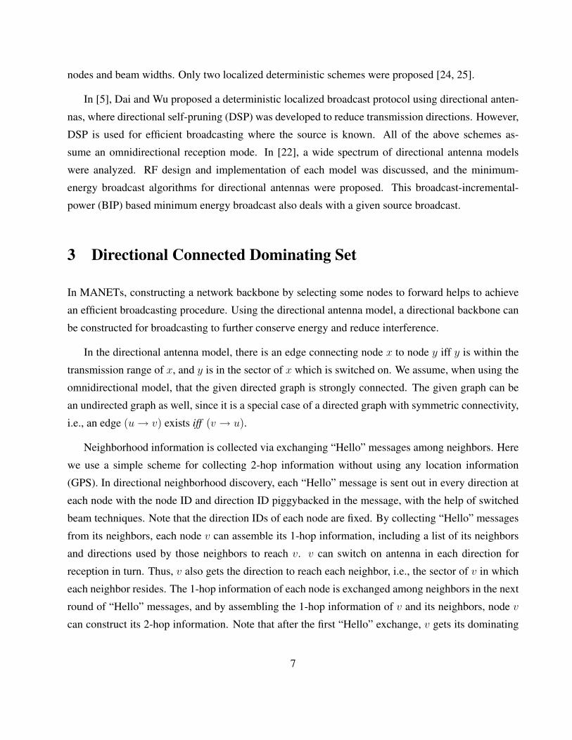
Figure 5: An example of DCDS by ECC.

There are two cases for the status of nodes on paths in RP .

Case 1: There is at least one path in RP with only marked nodes on it. Since RP connects u to w,

there is at least one edge on RP that is also in W . Then we assume edge (u′ → w′) is the edge on this

path and also in W . Therefore, p(u′ → w′) is larger than p(u → w). This contradicts the assumption

that (u → w) is the highest priority edge in area W .

Case 2: There is at least one unmarked node on each path in RP . As shown in (b), these unmarked

nodes form a rim W ′. We then assume node u′ has the highest priority in W ′. Since u′ is unmarked,

a replacement path, Pa, must exist for it based on the node coverage condition.

• There is at least one node on Pa, node u′′, which is also in W ′ (otherwise there is a path in RP

with only marked nodes). The priority of u′′ is higher than that of u′, which contradicts the

assumption that u′ is the highest one in W ′.

• There is no intermediate node on Pa. The dominating neighbor of u′ is connected to its ab-

sorbent neighbor on Pa; (a → b) exists. If a 6= u or b 6= w, u′ can be removed from Pa. If

15

Algorithm 2 SO algorithm

Align the edge of one sector to each selected forwarding edge, and determine the one with the

smallest number of switched-on sectors.

a = u, b = w, since u′ is unmarked, p(a) = p(u) > p(u′), which contradicts the assumption

that p(u′ → w) > p(u → w) (edge (u′ → w) is on Pa).

All of the contradictions above show that there exists a path connecting s to d with only marked

nodes and edges. 2

From the above proof we can see why the second condition of the node coverage condition is

necessary. In Figure 4 (b), when a = u, and b = w and p(u′) > p(a) = p(u) (thus edge (u → w) can

be unmarked based on the edge coverage condition), if u′ can be unmarked based on the node coverage

condition without the condition that p(a) = p(u) > p(u′) as case in (2), u′ and edge (u → w) are

unmarked simultaneously.

Figure 5 shows a large scale example in a 10× 10 area. There are 30 nodes, and the transmission

range is 3. The resultant DCDS is shown as dark nodes and dark arrows. In the resultant graph,

there are 13 forwarding nodes and 47 forwarding edges. All the directed neighbors of node 21 are

connected to one another. For example, node 21 has the highest priority (the larger the node ID, the

higher the node priority) in its local area. Thus, using the node coverage condition, it is a forwarding

node. The same can be said for node 23.

4.2 Sector Optimization (SO)

After the directional edges are determined for each forwarding node, the transmission directions can

be calculated based on the given number of sectors K. We also assume that the sectors of the direc-

tional antenna of each node are not necessarily aligned. We can develop an optimization algorithm to

let each node circumgyrate its antennas to minimize the number of its switched-on sectors. The sector

optimization algorithm (SO) is shown in Algorithm 2.

In Figure 6, K = 4, and the forwarding node has four forwarding edges. The antenna sectors are

circumgyrated to align with each edge. In cases (c) and (d) there are a smaller number of switched-on

sectors. The time complexity is the number of forwarding edges, |E ′v| (dominating edges of node v in

16

(d)

p

q

(a) (b) (c)

x

y

Figure 6: Illustration of SO.

E ′).

4.3 Property of ECC

We have shown the correctness of the proposed algorithm. We prove its effectiveness in this subsec-

tion.

We can easily show that the node coverage condition produces a smaller CDS than a known

condition called Rule k [4]. Our previous work has proven that the expected number of marked

nodes in Rule k is bound by O(1)|CDSopt|. This is also an upper bound for the total number of

marked nodes in ECC algorithms. When an ideally sectorized antenna model with K sectors is used,

the expected number of transmission directions is O(K)|CDSopt|. Note that the above argument is

applicable before the edge coverage condition is applied.

Theorem 3 Given an ideally sectorized antenna model with K sectors, the expected performance of

the ECC algorithm is O(K) times greater than in an optimal solution in random MANETs.

Proof: Both the coverage condition, directed or undirected, and the node coverage condition produce

a smaller CDS than a known condition called Rule k [4] with the assumption that nodes are randomly

distributed to generate the geometric graph. In Rule k, a node v can be unmarked if all its neighbors

are interconnected via k (k ≥ 1) nodes with higher priorities than v. Obviously this condition is

stronger than both the coverage condition and the node coverage condition. Our previous work has

proven that the expected number of marked nodes in Rule k is bounded by O(1)|CDSopt|. This is also

17

(b)

x v

u

w

(a)

u x

v

w

Figure 7: (a) A DCDS after the first round, (b) the reduced DCDS after the second round.

an upper bound for the total number of marked nodes in the proposed algorithms. When an ideally

sectorized antenna model with K sectors is used, the expected number of transmission directions is

E[TDN ] = O(K)|CDSopt|. (1)

Then we consider an optimal solution with the minimal number of transmission directions TDNopt.

For convenience, we denote any node with at least one transmission direction a marked node. Obvi-

ously, all marked nodes form a CDS, denoted as CDSTD, and

|CDSopt| ≤ |CDSTD| ≤ TDNopt. (2)

Combining (1) and (2), we have E[TDN ] = O(K)TDBopt. The probabilistic bound is based on K.

Usually, K is a constant value, O(K) = O(1). Therefore, E[TDN ] = O(1)TDBopt. 2

5 Extensions

In this section, two extensions are proposed to further improve the energy efficiency of the proposed

algorithm.

5.1 Iterative DCDS

As mentioned above, one of the drawbacks of all priority-based schemes is that they may select a

large CDS based on a bad priority assignment. In the previous algorithms, a fixed priority of each

node is used.

18

Algorithm 3 k-round ECC-I algorithm

1. Execution of ECC.

2. Exit if the number of iterations reaches k; otherwise, each node selects a new priority and

exchanges status (and priority if needed) with neighbors.

3. Apply ECC again on marked nodes/edges. Only marked nodes/edges can be used as coverage

nodes/edges to unmark other marked nodes/edges. Go to step 2.

To avoid simultaneous withdrawals, and the problem of a large selected set due to a bad priority

assignment exists.

Inspired by the iterative local approach of [33], we extend the proposed algorithm to iterative

versions to mitigate the side effect of priority assignment.

In the proposed algorithm, which depends on node priority, some priority rotation schemes can be

applied to generate a new priority for each node, and then the algorithm can be performed again. The

number of iterations does not need to be too large, as proved in [33]. Then the algorithm can go on to

execute the following steps. Algorithm 3 is the iterative version of ECC (ECC-I).

For the priority rotation scheme we can choose from shifting, shuffling, or random as proposed

in [33]. We can also associate the priority with the energy level of the node to make nodes with

higher energy marked easily. For example, we can use (energy level, random number) as node

priority. [33] also proposed a seamless iterative local solution for the dynamic environment via a

special priority designation which can also be applied in our algorithms. As the example shown in

Figure 7. (a) is a resultant ECDS after ECC. We assume that using some priority rotation scheme, the

node priorities change to what is shown in (b). Thus, the edge (x → v) can be unmarked. (b) is the

reduced DCDS after the second round of ECC-I.

5.2 DCDS for Topology Control

The previous proposed algorithm for DCDS helps each node to set several transmission directions.

Compared with each one using omnidirectional antennas to connect to every neighbor, DCDS helps

to preserve energy consumption. In order to further control energy consumption, we can try to control

the transmission range of each direction as in the topology control method of omnidirectional trans-

mission. We name the topology control by ECC algorithm as ECC-TC, as shown in Algorithm 4.

19

Algorithm 4 ECC-TC algorithm

1. Use ECC to mark forwarding nodes and their forwarding edges.

2. Use “SO” to determine switched-on sectors of each forwarding node.

3. In each switched-on sector, set the transmission range to reach the farthest neighbor connected

by a forwarding edge in this sector.

Compared with the energy-efficient broadcast protocol proposed in [12] where the dominating set

is constructed from the result of the LMST-based topology control according to the “optimal radius”,

ECC-TC first constructs the DCDS. Then it applies topology control, setting up not only transmission

ranges, but also transmission directions. In Figure 6 (d), final transmission ranges should be set to

reach nodes x and q in the switched-on sectors, respectively.

6 Simulation

We evaluate the proposed algorithm ECC, and its extensions, iterative DCDS (ECC-I) and DCDS

with topology control (ECC-TC) via two groups of simulations conducted on a custom simulator

and also the network simulator ns2 [7]. In the first group, we focus on the performance analysis by

comparing the DCDS generated by the proposed algorithms with the traditional CDS using omnidi-

rectional models in terms of the number of forwarding nodes, forwarding edges, switched-on sectors,

and total power consumption in ideal networks without packet loss. In the second group, we analyze

the efficiency and reliability of these algorithms when there are collision and mobility. We use two

approaches to generate CDS, Rule k and a coverage condition (Generic).

6.1 Simulation Environment

To generate a random network, n nodes are randomly placed in a restricted 100× 100 area. Networks

that cannot form a strongly connected graph are discarded. The tunable parameters in the simulation

are as follows. (1) The number of nodes n. We vary the number of deployed nodes from 20 to 160

to check the scalability of the algorithms. (2) The transmission range r. In order to generate directed

20

8

10

12

14

16

18

20

22

24

20 40 60 80 100 120 140 160

Num

ber

of F

orw

ardi

ng N

odes

Number of Nodes

Rule kGeneric

ECC

(a) Forwarding nodes

0

200

400

600

800

1000

1200

20 40 60 80 100 120 140 160

Num

ber

of F

orw

ardi

ng E

dges

Number of Nodes

Rule kGeneric

ECC

(b) Forwarding edges

30

40

50

60

70

80

90

20 40 60 80 100 120 140 160

Num

ber

of S

witc

hed-

on S

ecto

rs

Number of Nodes

Rule kGeneric

ECC

(c) Switched-on sectors (K = 4)

40

50

60

70

80

90

100

110

120

130

140

20 40 60 80 100 120 140 160

Num

ber

of S

witc

hed-

on S

ecto

rs

Number of Nodes

Rule kGeneric

ECC

(d) Switched-on sectors (K = 6)

Figure 8: Comparison of Rule k, Generic, and ECC in directional graphs.

graphs, each node randomly picks its transmission range from 20 to 40. (3) The number of sectors of

the antenna pattern K. We use 4 and 6 as the values of K. (4) The number of hops h. In coverage

condition, 2, 3, or 4 hops local information is collected for our localized algorithms. (5) The maximal

forward jitter delay d. We vary it from 0.01 to 100 ms. (6) The average moving speed v. When there

is mobility, the average moving speed is varied from 1 to 25 m/s. The first four parameters are for the

ideal network simulation and the last two are for the realistic network simulation.

The following metrics are compared: (1) the number of forwarding nodes, (2) the number of

forwarding edges, (3) the total energy consumption when used as topology control, (4) the energy

reduction ratio, and (5) the delivery ratio of broadcast message in the realistic simulation. The power

consumption in ECC-TC is calculated according to the algorithm, and we use the square of the trans-

mission range as the power consumption in one sector.

21

6

8

10

12

14

16

18

20

20 40 60 80 100 120 140 160

Num

ber

of F

orw

ardi

ng N

odes

Number of Nodes

Rule kGeneric

ECC

(a) Forwarding nodes

0

200

400

600

800

1000

1200

1400

20 40 60 80 100 120 140 160

Num

ber

of F

orw

ardi

ng E

dges

Number of Nodes

Rule kGeneric

ECC

(b) Forwarding edges

20

30

40

50

60

70

80

20 40 60 80 100 120 140 160

Num

ber

of S

witc

hed-

on S

ecto

rs

Number of Nodes

Rule kGeneric

ECC

(c) Switched-on sectors (K = 4)

40

50

60

70

80

90

100

110

120

20 40 60 80 100 120 140 160

Num

ber

of S

witc

hed-

on S

ecto

rs

Number of Nodes

Rule kGeneric

ECC

(d) Switched-on sectors (K = 6)

Figure 9: Comparison of Rule k, Generic, and ECC in undirected graphs (r = 40).

6.2 Simulation Results From Custom Simulator

Figure 8 shows the comparison of Rule k [4] and Generic [32] which generate the CDS, and the ECC

algorithm which generates the DCDS. h is 2 in the following simulations unless specified. In (a) the

number of forwarding nodes of ECC is larger than Generic. Rule k is less efficient than Generic, so

it generates a larger CDS, especially when the network is very dense. (b) is the comparison of the

number of forwarding edges. In Rule k and Generic, all the dominating edges of forwarding nodes are

their forwarding edges. ECC has a much smaller number of forwarding edges than CDS, especially

when n is large. Figures 8 (c) and (d) show the numbers of switched-on sectors in Rule k and Generic

(all sectors of each forwarding node are switched-on due to the omnidirectional antenna), and ECC,

when K is 4 and 6 respectively.

Figure 9 shows the results of the three algorithms when the original graph is undirected (r = 40).

22

10

12

14

16

18

20

22

20 40 60 80 100 120 140 160

Num

ber

of F

orw

ardi

ng N

odes

Number of Nodes

h=2h=3h=4

(a) Forwarding nodes

0

50

100

150

200

250

300

20 40 60 80 100 120 140 160

Num

ber

of F

orw

ardi

ng E

dges

Number of Nodes

h=2h=3h=4

(b) Forwarding edges

Figure 10: ECC performance with different h.

(a) shows the selected forwarding nodes, (b) is the forwarding edges, and (c) and (d) are the switched-

on sectors when K is 4 and 6, respectively. Compared with Figure 8, a larger transmission range

and more links lead to a smaller forwarding node set for all four algorithms. However, Rule k and

Generic have larger forwarding edge sets because each forwarding node tends to have more edges.

ECC has a smaller forwarding edge set than those in Figure 8. In (c) and (d), Rule k and Generic have

smaller switched-on sectors than in Figure 8 due to the reduced number of forwarding nodes. Since

the relative performance of the four algorithms is the same as in directed graph, we set the original

graph to be directed in the following without loss of generality.

Figure 10 shows the performance ECC with different h values. (a) and (b) show the numbers of

forwarding nodes and edges in the DCDS, with 2, 3, and 4 hops local information. We can see that,

with more local information, the smaller DCDS can be achieved in terms of both forwarding nodes

and edges. However, when h increases from 3 to 4, the performance improvement is not significant.

Thus, a relatively small h is appropriate for the localized ECC. In ECC, the increase of h helps to

reduce both forwarding nodes and forwarding edges.

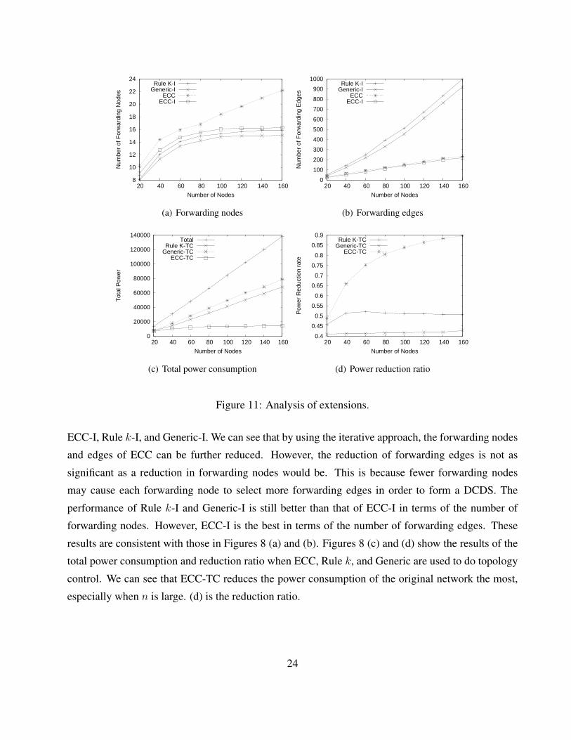
Figure 11 shows the performance analysis of the two extensions. Rule k and Generic are also

extended to iterative versions (Rule k-I and Generic-I) and applied for topology control purposes (Rule

k-TC and Generic-TC). In Rule k-TC and Generic-TC, a dominating and absorbent set is constructed

using Rule k or Generic. Then, each marked node sets its transmission range to reach its farthest

neighbor and each unmarked node sets its transmission range to reach its nearest marked neighbor.

(a) and (b) show the comparison of the numbers of forwarding nodes and forwarding edges in ECC,

23

8

10

12

14

16

18

20

22

24

20 40 60 80 100 120 140 160

Num

ber

of F

orw

ardi

ng N

odes

Number of Nodes

Rule K-IGeneric-I

ECCECC-I

(a) Forwarding nodes

0

100

200

300

400

500

600

700

800

900

1000

20 40 60 80 100 120 140 160

Num

ber

of F

orw

ardi

ng E

dges

Number of Nodes

Rule K-IGeneric-I

ECCECC-I

(b) Forwarding edges

0

20000

40000

60000

80000

100000

120000

140000

20 40 60 80 100 120 140 160

Tot

al P

ower

Number of Nodes

TotalRule K-TC

Generic-TCECC-TC

(c) Total power consumption

0.4

0.45

0.5

0.55

0.6

0.65

0.7

0.75

0.8

0.85

0.9

20 40 60 80 100 120 140 160

Pow

er R

educ

tion

rate

Number of Nodes

Rule K-TCGeneric-TC

ECC-TC

(d) Power reduction ratio

Figure 11: Analysis of extensions.

ECC-I, Rule k-I, and Generic-I. We can see that by using the iterative approach, the forwarding nodes

and edges of ECC can be further reduced. However, the reduction of forwarding edges is not as

significant as a reduction in forwarding nodes would be. This is because fewer forwarding nodes

may cause each forwarding node to select more forwarding edges in order to form a DCDS. The

performance of Rule k-I and Generic-I is still better than that of ECC-I in terms of the number of

forwarding nodes. However, ECC-I is the best in terms of the number of forwarding edges. These

results are consistent with those in Figures 8 (a) and (b). Figures 8 (c) and (d) show the results of the

total power consumption and reduction ratio when ECC, Rule k, and Generic are used to do topology

control. We can see that ECC-TC reduces the power consumption of the original network the most,

especially when n is large. (d) is the reduction ratio.

24

0

10

20

30

40

50

60

70

80

90

100

20 40 60 80 100 120 140 160

Per

cent

age

of S

witc

hed-

on S

ecto

rs

Number of Nodes

FloodingRule k

GenericECC

(a) Percentage of switched-on sectors

90

92

94

96

98

100

20 40 60 80 100 120 140 160

Del

iver

y R

atio

Number of Nodes

FloodingRule k

GenericECC

(b) Delivery versus number of nodes

60

65

70

75

80

85

90

95

100

0.01 0.1 1 10 100

Del

iver

y R

atio

Maximal Forward Jitter Delay

FloodingRule k

GenericECC

(c) Delivery versus forward jitter

70

75

80

85

90

95

100

0 5 10 15 20 25

Del

iver

y R

atio

Average Moving Speed

FloodingRule k

GenericECC

(d) Delivery versus moving speed

Figure 12: Performance in realistic networks with collision and mobility (K = 4, h = 3).

6.3 Simulation Results From ns2

In previous simulation, we focused on the performance analysis of DCDS in terms of the number

of forwarding nodes, forwarding edges, switched-on sectors, and total power consumption in our

custom ideal networks. Next, we will study the efficiency and reliability of the algorithm in a realistic

environment simulated by ns2 when there is collision and mobility.

Figure 12 shows the simulation results using ns2.1b9. We use the directional antenna model and

an enhanced IEEE 802.11 MAC layer provided by the enhanced network simulator (TeNs) [23]. We

simulate the proposed ECC algorithm together with the blind flooding (Flooding) and Rule k and

Generic algorithms to study their efficiency and reliability as functions of the network size, collision

and mobility. K is 4 and h is 3 in the following simulation. The nodes share a single 2MB channel,

and the traffic load is 1-10 packets per second (pps) with a packet size of 64 bytes. The “Hello”

25

message interval is 1s. We use the random waypoint mobility model [18].

Figure 12 (a) shows the percentage of total switched-on sectors with different network sizes

(v = 1, d = 100). We can see that Flooding switches on almost all sectors for transmission, ex-

cept when n is quite small and the percentage of nodes that do not receive the packet due to collision

and do not forward is relatively significant. All the other three algorithms have smaller percentages

which decrease as the number of nodes increases. Among them, ECC has the smallest percentage of

switched-on sectors and Rule k has the largest. These results are consistent with those in the ideal

network simulation.

Figures 12 (b)-(d) show the reliability in terms of delivery ratio. (b) is with a different network

size (v = 1, d = 100). Flooding achieves almost 100% delivery ratio, especially when the network

size is larger than 40. The other three have lower delivery ratios, and among them, ECC has the

best performance. (c) is with different forward jitter delay (n = 100, v = 1). In order to reduce the

collision caused by the directional hidden terminal problem, we use a random forward jitter delay

in the simulation which is within range [0, dmax]. We can see that when the jitter delay is small,

for instance, dmax = 0.01 − 0.1ms, the delivery ratios of all the algorithms are very low, including

Flooding. When dmax increases to 1, the delivery ratios are around 95%. When dmax is 100, the

delivery ratios reach the previous results as in (b). However, the increase of dmax leads to the increase

of the average end-to-end delay, too. (d) has a different average moving speed (n = 100, d = 100).

Flooding is not affected by the mobility significantly due to its large redundancy. All the other three

have lower delivery ratios when the speed at which the nodes move increases. Among the three,

Rule k has the largest delivery ratio when v is relatively large. This is because Rule k has the largest

redundancy. However, the difference is quite small.

These four approaches present different tradeoffs between energy efficiency and robustness. Blind

flooding tolerates the node mobility the most while being the least efficient one. By developing the

ECC, we are trying to exploit the other extreme on the spectrum, superior efficiency but only for

low-mobility networks.

6.4 Summary

Simulation results in this section can be summarized as follows:

26

1. ECC generates a DCDS with fewer forwarding edges than the Rule k and the coverage condition

algorithms.

2. Using directional antennas, the number of switched-on sectors in ECC is smaller than those

using omnidirectional antennas.

3. More local information helps to improve the performance of ECC, but a relatively small h is

sufficient.

4. ECC-I can improve the performance of ECC; ECC-TC reduces the total power consumption of

the original network significantly.

5. In a realistic network with collision, ECC outperforms Rule k and the coverage condition in

terms of both efficiency and reliability.

6. With movement in the network, Rule k and the coverage condition algorithms are slightly better

than ECC.

7 Conclusions

In this paper, we put forward the concept of directional network backbone. Using directional antennas,

constructing a directional network backbone in MANETs can further reduce total energy consumption

as well as reduce interference in broadcasting applications. A two-phase approach for the directional

backbone is developed. First we construct a directional connected dominating set (DCDS), which

is an extreme case of directional backbone, then selected edges in the DCDS are combined to form

switched-on sectors. A heuristic localized algorithm for constructing a small DCDS is proposed,

which is a non-trivial extension of the existing approaches for the regular dominating set problem.

The sector optimization algorithm is developed for the second phase. Then two extensions of the

proposed algorithm are discussed. One is the iterative version, and the other is the application which

incorporates topology control. Performance analysis are conducted, including a theoretical analysis

in terms of the approximation ratio and simulations of the proposed algorithms. In the future, we

will develop localized solutions for the directional network backbone problem directly, instead of a

two-phase approach. We will also analyze the energy consumption issue in this problem, considering

a practical energy model.

27

8 Acknowledgement

This work was supported in part by NSF grants ANI 0083836, CCR 0329741, CNS 0422762, CNS

0434533, EIA 0130806, CNS 0531410, and CNS 0626240. The authors thank the reviewers for their

constructive comments and Alex Zelikovsky for his insightful comments on this paper.

References

[1] J. Carle and D. Simplot-Ryl. Energy-efficient area monitoring for sensor networks. IEEE Computer,

(2):40–46, 2004.

[2] R. R. Choudhury and N. H. Vaidya. Ad hoc routing using directional antennas, Technical report, Dept. of

Electrical and Computer Engineering, University of Illinois at Urbana Champaign. 2002.

[3] R. R. Choudhury, X. Yang, R. Ramanathan, and N. H. Vaidya. Using directional antennas for medium

access control in ad hoc networks. In Proc. of ACM/SIGMOBILE MobiCom, 2002.

[4] F. Dai and J. Wu. An extended localized algorithm for connected dominating set formation in ad hoc

wireless networks. IEEE Transaction on Parallel and Distributed Systems, 15(10):908–920, 2004.

[5] F. Dai and J. Wu. Efficient broadcasting in ad hoc wireless networks using directional antennas. IEEE

Transactions on Parallel and Distributed Systems, (4):1–13, 2006.

[6] B. Das, R. Sivakumar, and V. Bharghavan. Routing in ad-hoc networks using a spine. In Proc. of IC3N,

1997.

[7] K. Fall and K. Varadhan. The NS manual. The VINT Project, UCB, LBL, USC/ISI, and Xerox PARC,

http://www.isi.edu/nsnam/ns/doc/, 2002.

[8] G. N. Frederickson and J. JaJa. Approximation algorithms for several graph augmentation problems.

SIAM Journal on Computing, (2):270–283, 1981.

[9] S. Guha and S. Khuller. Approximation algorithms for connected dominating sets. Algorithmica,

20(4):374–387, 1998.

[10] P. Gupta and P. R. Kumar. Capacity of wireless networks. IEEE Transcations on Information Theory,

pages 388–404, 2000.

28

[11] C. Hu, Y. Hong, and J. Hou. On mitigating the broadcast storm problem with directional antennas. In

Proc. of IEEE ICC, 2003.

[12] F. Ingelrest, D. Simplot-Ryl, and I. Stojmenovic. Optimal transmission radius for energy efficient broad-

casting protocols in ad hoc and sensor networks. IEEE Transactions on Parallel and Distributed Systems,

(6):536–547, 2006.

[13] A. Keshavarz-Haddad, V. Ribeiro, and R. Riedi. Broadcast capacity in multihop wireless networks. In

Proc. of ACM/SIGMOBILE MobiCom, 2006.

[14] P. H. Lehne and M. Petterson. An overview of smart antenna technology for mobile communications

systems. IEEE Communications Surveys and Tutorials, (4):388–404, 1999.

[15] L. Li, R. Ramjee, M. Buddhikot, and S. Miller. Network coding-based broadcast in mobile ad hoc net-

works. In Proc. of IEEE INFOCOM, 2007.

[16] H. Liu, Y. Pan, and J. Cao. An improved distributed algorithm for connected dominating sets in wire-

less ad hoc networks. In Proc. of International Symposim on Parallel and Distributed Processing and

Applications (ISPA), Lecture Notes in Computer Science, number 3358, 2004.

[17] W. Lou and J. Wu. On reducing broadcast redundancy in ad hoc wireless networks. IEEE Transactions

on Mobile Computing. 1(2):111-122, April-June 2002.

[18] W. Navidi and T. Camp. Stationary distributions for the random waypoint mobility model. IEEE Trans-

actions on Mobile Computing, (1):99–108, 2004.

[19] C. H. Papadimitriou and U. V. Vazirani. On two geometric problems related to the traveling salesman

problem. Journal of Algorithms, (2):231–246, 1984.

[20] A. Qayyum, L. Viennot, and A. Laouiti. Multipoint relaying for flooding broadcast message in mobile

wireless networks. In Proc. of 35th Hawaii Int’l Conf. on System Sciences (HICSS-35), 2002.

[21] R. Ramanathan. On the performance of ad hoc networks with beamforming antennas. In Proc. of ACM

MobiHoc, 2001.

[22] S. Roy, Y. C. Hu, D. Peroulis, and X.-Y. Li. Minimum-energy broadcast using practical directional

antennas in all-wireless networks. In Proc. of IEEE INFOCOM, 2006.

[23] S. Roy and A. Kumar. Realistic support for IEEE 802.11b MAC in NS. Bachelor’s thesis, Indian Inst.

of Technology, Kanpur, 2004.

29

[24] C. C. Shen, Z. Huang, and C. Jaikaeo. Directional broadcast for ad hoc networks with percolation theory,

technical report, Computer and Information Sciences, University of Delware. 2004.

[25] D. Simplot-Ryl, J. Cartigny, and I. Stojmenovic. An adaptive localized scheme for energy efficient broad-

casting in ad hoc networks with directional antennas. In Proc. of 9th IFIP PWC, 2004.

[26] P. Sinha, R. Sivakumar, and V. Bharghavan. CEDAR: a core-extraction distributed ad hoc routing al-

gorithm. IEEE Journal on Selected Areas in Communications, Special Issue on Ad Hoc Networks,

17(8):1454–1465, Aug. 1999.

[27] Y. C. Tseng, S. Y. Ni, Y. S. Chen, and J. P. Sheu. The broadcast storm problem in a mobile ad hoc network.

Wireless Networks, (2-3):153–167, 2002.

[28] P. J. Wan, K. Alzoubi, and O. Frieder. Distributed construction of connected dominating set in wireless

ad hoc networks. In Proc. of IEEE INFOCOM, 2002.

[29] J. E. Wieselthier, G. D. Nguyen, and A. Ephremides. Energy-aware wireless networking with directional

antennas: the case of session-based broadcasting and multicasting. IEEE Transactions on Mobile Com-

puting, (3):176–191, 2002.

[30] J. H. Winters. Smart antenna techniques and their application to wireless ad hoc networks. IEEE Wireless

Communications, (4):77– 83, 2006.

[31] J. Wu. Extended dominating-set-based routing in ad hoc wireless networks with unidirectional links.

IEEE Transactions on Parallel and Distributed Computing, (1-4):327–340, 2002.

[32] J. Wu and F. Dai. A generic distributed broadcast scheme in ad hoc wireless networks. IEEE Transactions

on Computers, (10):1343–1354, 2004.

[33] J. Wu, F. Dai, and S. Yang. Iterative local solution for connected dominating set in ad hoc wireless

networks. In Proc. of IEEE MASS, 2005.

[34] J. Wu and H. Li. On calculating connected dominating sets for efficient routing in ad hoc wireless net-

works. In Proc. of ACM DIALM’99, 1999.

[35] J. Wu and W. Lou. Forward-node-set-based broadcast in clustered mobile ad hoc networks. Wireless

Networks and Mobile Computing, a Special Issue on Algorithmic, Geometric, Graph, Combinatorial, and

Vector Aspects, 3(2):155–173, 2003.

[36] S. Yi, Y. Pei, and S. Kalyanaraman. On the capacity improvement of ad hoc wireless networks using

directional antennas. In Proc. of ACM MobiHoc, 2003.

30