������������� �����

�������� ������������

Dipl.-Ing. Michael Ehlen

Fluent Deutschland GmbH

CFD Konferenz 2004 in Bingen

������ ���� �������������!�"�

���

# �� ���� �������������!�"����$

� A method by which the solver (FLUENT) can be instructed to moveboundaries and/or objects, and to adjust the mesh accordingly

� Examples:� Automotive piston

moving inside a cylinder

� A flap moving on an airplane wing

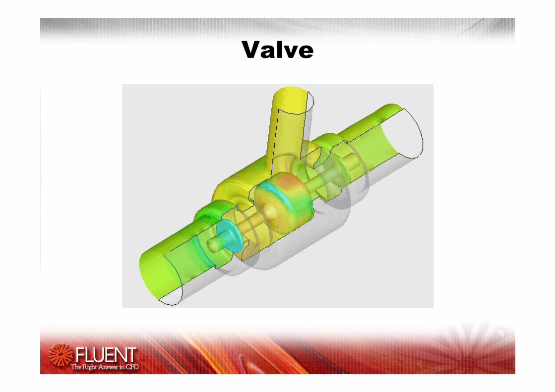
� A valve opening and closing

Volumetric fuel pump

Animati

on

# ������ ����������������$

• Used when rigid boundaries move with respect to each other, e.g.,

– Piston moving w.r.t. an engine cylinder (linear motion)– Flap moving w.r.t. an airplane wing (rotating motion)

• Used when boundaries deform/deflect, e.g.,

– A balloon that is being inflated– A solid propellant retreating as it is being consumed by the flame– The shrinking or extending walls of an engine cylinder as the piston

moves in and out

�����������!�"����%�������

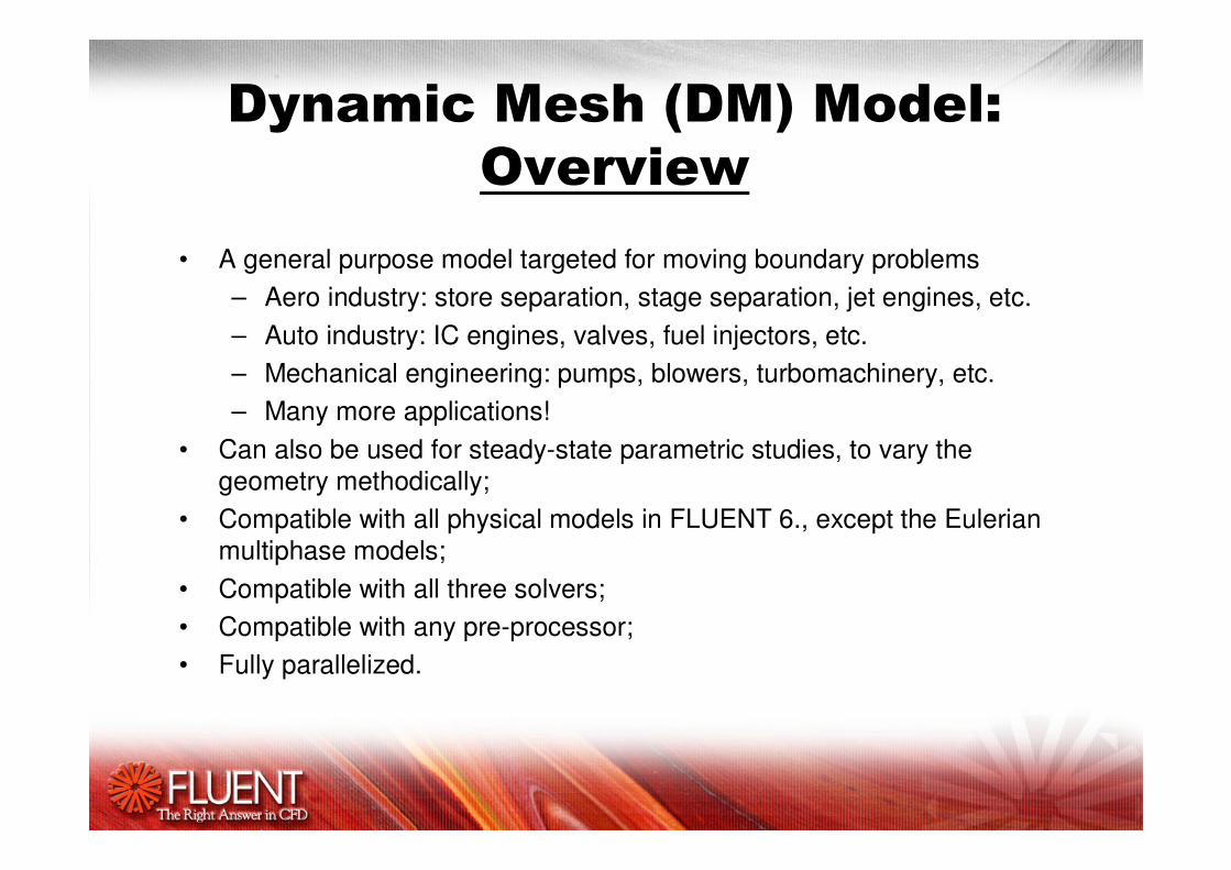
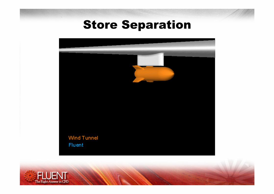
• A general purpose model targeted for moving boundary problems– Aero industry: store separation, stage separation, jet engines, etc.– Auto industry: IC engines, valves, fuel injectors, etc.– Mechanical engineering: pumps, blowers, turbomachinery, etc.– Many more applications!

• Can also be used for steady-state parametric studies, to vary the geometry methodically;

• Compatible with all physical models in FLUENT 6., except the Eulerian multiphase models;

• Compatible with all three solvers;• Compatible with any pre-processor;• Fully parallelized.

�����������!�"����%� � ���

• Several meshing schemes are available to handle all types of boundary motion;

• Boundaries/Objects may be moved based on:– In-cylinder motion (RPM, stroke length, crank angle, …);– Prescribed motion via profiles;– Prescribed motion via UDF (User-Defined Function);– Coupled motion based on hydrodynamic forces from the flow solution,

via FLUENT’s 6 DOF model.

�����%����� ����&����

• Fluent’s DM (Dynamic Mesh) model offers three meshing schemes:

– Spring analogy (smoothing);

– Local remeshing;

– Layering.

• Mesh motion may be applied to individual zones;• Different zones may use different schemes for mesh motion;• Connectivity between adjacent deforming zones may be non-conformal, e.g.,

there might be a sliding interface between two neighboring zones.

&'���(������(��!&'���(�&��� ���("

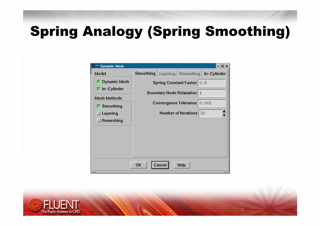
• The nodes move as if connected via springs, or as if they were part of a sponge;

• Connectivity remains unchanged;• Limited to relatively small

deformations when used as a stand-alone meshing scheme;

• Available for tri and tet meshes;• May be used with quad, hex and

wedge mesh element types, but that requires a special command;

Animati

on

������)�����(

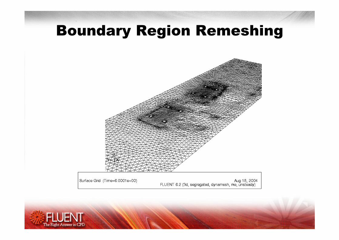
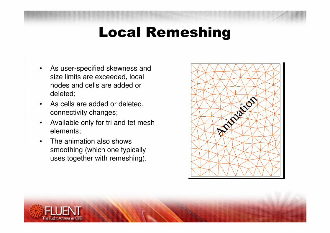
• As user-specified skewness and size limits are exceeded, local nodes and cells are added or deleted;

• As cells are added or deleted, connectivity changes;

• Available only for tri and tet mesh elements;

• The animation also shows smoothing (which one typically uses together with remeshing).

Animati

on

������(

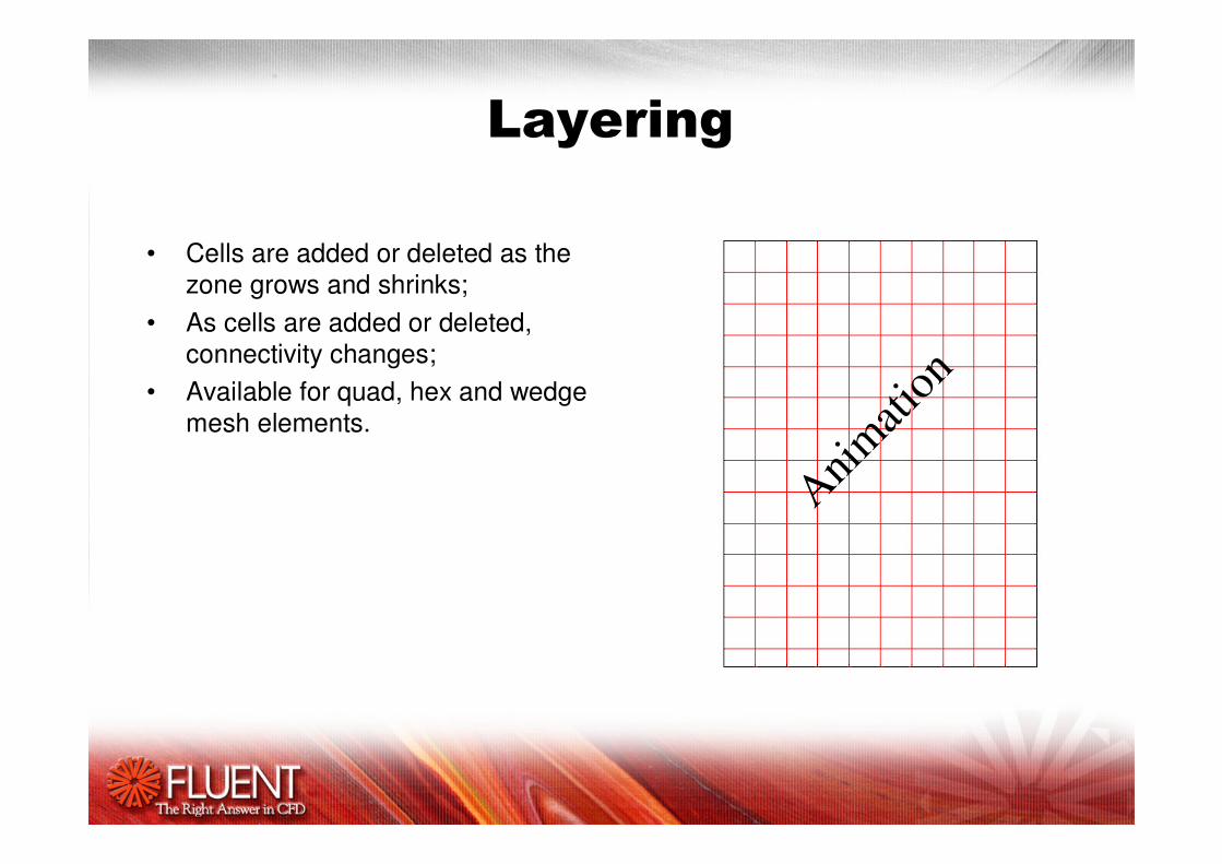
• Cells are added or deleted as the zone grows and shrinks;

• As cells are added or deleted, connectivity changes;

• Available for quad, hex and wedge mesh elements.

Animati

on

������(Bottom Layering Top Layering

Settings:- wall (bottom): rigid body

Settings:- fluid (hex): rigid body - interior zone: stationary- wall (bottom): rigid body

fluid (hex)

interior zone

wall (bottom)

*������ ��������''������

• Initial mesh needs proper decomposition;

• Layering:– Valve travel

region; – Lower cylinder

region.• Remeshing:

– Upper cylinder region.

• Non-conformal interface between zones.

Animati

on

+�,�!+��'����������,� ����"

• Define > Dynamic Mesh > Parameters

– Select “Dynamic Mesh” to enable the model, then select one or more specific mesh method: spring smoothing, layering, and/or local remeshing;

– The “In-Cylinder” option is for easily defining the motion of pistons and valves.

� ����&'������ ���

• The motion of certain boundaries or fluid zones is specified via Define > Dynamic Mesh > Zones

• The example shows a wall called “rotor_clock” that moves as a rigid body according to a UDF called “clockwise”: the example is for a gear that spins clockwise about its C.G. (center of gravity).

&'���(������(��!&'���(�&��� ���("

������)�����(

������(��-��'��.%�/�� ��

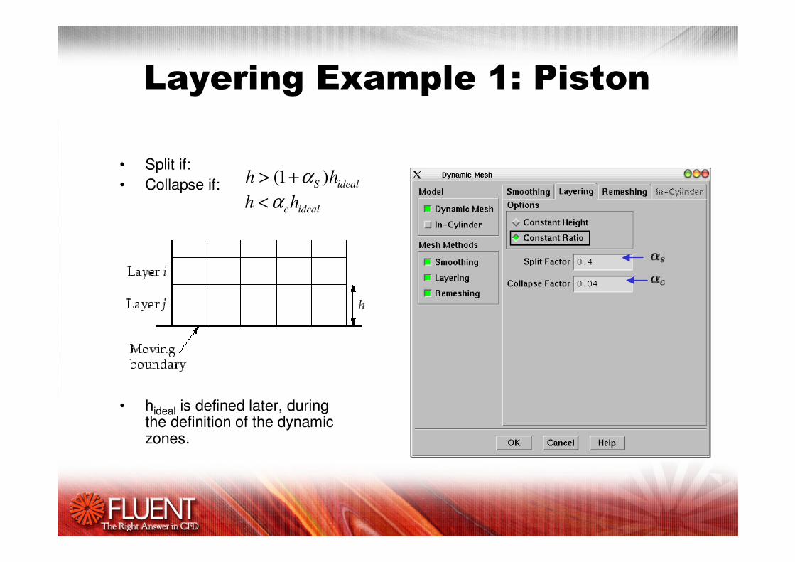
• Split if: • Collapse if:

• hideal is defined later, during the definition of the dynamic zones.

idealS hh )1( α+>idealchh α<

������(• Constant Height:

– Every new cell layer has the same height;

• Constant Ratio: – Maintain a constant ratio of cell

heights between layers (linear growth);

– Useful when layering is done in curved domains (e.g. cylindrical geometry).

Initially, piston at

bottom-most position

Piston at top-most position

Edge “i”

Edges “i” and “i+1” have same shape

Edge “i+1” is an average of edge “i” and the piston shape

Constant Height

Constant Ratio

������(

• Definition of the dynamic zone:

piston (wall zone) moves as a rigid body in the y-direction

������(• Definition of the ideal

height of a cell layer;• hideal is about the same

as the height of a typical cell in the model.

� ����&'������ ���

• Internal node positions are automatically calculated based on user specified boundary motion:

• Prescribed mesh motion:

– Position or velocity versus time, i.e., ‘profile’ text file;– UDF with expression for position or velocity versus time

(independent of the flow solution).• Flow dependent motion (coupled motion):

– Mesh motion is coupled with the flow solution through a UDF;– One can compute forces (pressure, gravity, viscous, etc.) on a body

to arrive at its translational and rotational velocity components;– Six degree of freedom (6DOF) UDF provided;– UDF readily customized for desired mesh motion.

���/����

• Mesh motion can be previewed without calculating flow variables:– Allows user to quickly check mesh quality throughout the simulation

cycle;– Applicable to any dynamic mesh simulation;– Accessed via GUI: Solve > Mesh Motion;– Be careful with the time step.– Save your case before doing the preview, else the setup will be lost!

�����������!�"����%������ � ����

• Objects may not move from one fluid zone into another;• Cannot (yet) be used in conjunction with hanging node adaption (including

dynamic adaption);• Constrained motion, such as a motion about a hinge, is only allowed if one

uses a UDF;• Bodies may not make contact, since that implies a change in topology; one

always leaves at least one layer of cells between bodies;• DPM (discrete phase model) particles cannot be released from moving

surfaces (but one could vary the injection location as a function of time).

�� ������������ � ������� ������012

213���)�����(4&��� ���(

• For mapable (2.5D; extruded) geometries in particular pumps

5��������)(����)�����(�

&��� ���)�����(�

• New in FLUENT 6.2:– Symmetric boundaries– Across multiple zones– Feature preservation

(e.g., corners are preserved)

– Non-closed loops

)�����(4&��� ���(�� � �������������' ���

Limitation: Dynamic adaption cannot be used in conjunction with layering or with boundary remeshing

������(�� �/�������

Also: layering is now possible in fluid zones with mixed cell types, provided the cell type does not change as one crosses from the layering zone to the adjacent zone(s).

����*��'� ����� ��� � ��6�

07�� �&����

• 6-DOF solver now built into the GUI;• GUI panels still do not provide for constraints (such as hinges),

but constrained motion is possible via UDF;• The dynamic mesh UDFs contain hooks for load

forces/moments;• Transformations can be customized (although we use a

transformation between local and global coordinate systems that is widely used in the aerospace and shipbuilding industries).

�������������� �

• Events based on time (not just based on the crank angle as before), and without having to use the in-cylinder tools (where they were called in-cylinder events);

• New events:– Activate/Deactivate cell zones– Change URF

• You can also use events to control the time step!

/�����������������,�'�����

0

20

40

60

80

100

120

140

Fluent 6.1 Fluent 6.2

1cyc

leF

low

Ru

n T

ime

(hrs

.)

1CPU 2CPU 1CPU 2CPU

- 12%

- 34%

5.4 days 4.5 days 4.83 days 3 days

• HP-Linux machine with 2.2GHz processor speed• No need to encapsulate the interfaces• Run time reduction depending on case• Can vary between 33%-40%

�� �,*�/���• IC specific setup panel

– Fewer inputs and more features than 6.1 panel – Automatic setup of activate/deactivate, variable time step size and

URFs – Three different pistons types are also automatically set up

• Pistons with enough room to put one layer to start with (1)• Flat pistons with tight squish combustion chamber (2)• Complex piston shape like GDI engines (3)

– User need not specify the meshing parameters in the panel• Meshing parameters automatically calculated by the journal

– Takes care of symmetry engine as well– Can read and write parameters into a file

• Becomes very handy if a slightly different setup is explored.

�� �,*�/���

Fluent 6.2 IC Panel

�-��'��

,�7*������

��

/�� ���*�����(

/�����(�*���

& ���&'��� ����

6���

���,�8� ��