Eileen Maturi1, Jo Murray2, Andy Harris3, Paul Fieguth4, John Sapper1

1 NOAA/NESDIS, U.S.A., 2 Rutherford Appleton Laboratory, U.K., 3 University of Maryland, U.S.A., 4 University of Waterloo, Canada

MISST 2006 Meeting Washington, D.C.

28 November, 2006

MULTI-SEA SURFACE TEMPERATURE ANALYSIS

28 November 2006 MISST Meeting Washington, D.C. 2

OBJECTIVE

• Develop estimation scheme for combining multi-satellite retrievals of sea surface temperature into a single analysis

• Apply complementary SST datasets available from polar orbiters, geostationary IR and microwave sensors

• Use the computing power available to implement this estimation scheme

28 November 2006 MISST Meeting Washington, D.C. 3

NOAA Requirements

1. Operational SST Analysis using POES and GOES SSTs

2. Daily Global 0.1°0.1° 6 hourly at 5 km at selected regions 3. Accurate global error characterization 4. Preservation of information about fronts5. Extendable to other SST datasets + scalable

For NWP, climate research, fisheries, coastal services…

28 November 2006 MISST Meeting Washington, D.C. 4

SELECTED SST DATASETS

• AVHRR: – 1-km resolution– global coverage, good-quality retrieval

• GOES:– 4-km resolution– good temporal coverage– resolve diurnal cycle

• FUTURE: Microwave SSTs (TMI, AMSR, WINDSAT)– Low-resolution– SST retrievals not made closer than ~100km of coast– Insensitive to clouds and aerosol– Some sensitivity to wind speed

28 November 2006 MISST Meeting Washington, D.C. 5

Data Quality Control

• The observational SST data are quality-controlled using a spatial temporally varying consistency check with the previous day's SST analysis– the thresholds vary by the error estimate in the analysis and

the estimate of SST variability

• Data are then averaged into the 0.1° and 5-km resolutions used in the analyses

• Inter-sensor bias estimation with the NOAA-17 daytime SSTs (with CLAVR-x cloud mask value=0) are chosen as the reference dataset

28 November 2006 MISST Meeting Washington, D.C. 6

METHODOLOGY

• Initial guess of SST background field• Initial guess of SST variability• Observations with well-characterized errors• Definition of relationship between

observational datasets (i.e. assume one or more bias terms which are spatially correlated)

28 November 2006 MISST Meeting Washington, D.C. 7

Multi-scaleOptimal Interpolation SST

• Optimal, rigorous way of combining SST observations from AVHRR and GOES-Imager

• Individual datasets are bias-corrected• Error estimates are dynamically updated from

one day to the next• “Multi-scale” means that high resolution is

achieved at relatively little computational cost (global analysis runs in 40 minutes on a single Dell cpu)

28 November 2006 MISST Meeting Washington, D.C. 8

DAILY SST UPDATE

• System dynamics predict – the new SST estimate – the associated error information.

• Assume that the ocean dynamics are very slow– apply a very simple dynamic model– each pixel independently evolving randomly

• This model implies a simple estimate prediction: T(t|t-1) = T(t-1|t-1)

• The initial SST is modified implicitly by introducing new measurements– the measurement at any time t consists of two independent

components – the SST observations T and the predicted error estimates

28 November 2006 MISST Meeting Washington, D.C. 9

Daily SST Update (Contd)

The new SST estimate is obtained by adding the estimated anomaly field to the previous SST estimate…

• Propagation of error statistics – achieved by appropriately down weighting the impact of

the previous SST estimate• by increasing the associated error variance • calculating error estimate based on both this error and

the observational error associated with the new observations

• Data preprocessing observational noise is empirically determined from each dataset– Vital to ensure the appropriate SST and error estimates

are used in the analysis

28 November 2006 MISST Meeting Washington, D.C. 10

Boundaries of Ocean Basins

28 November 2006 MISST Meeting Washington, D.C. 12

Treatment of individual SST datasets

Select AVHRR daytime as baseline SST:

SST = AVHRR (day) + observation (obs) noise

Other datasets are considered relative to this baseline:

SST = AVHRR (night) + diurnal warming + obs noiseSST = GOES (night) + atmospheric term + obs noiseSST = GOES (day)+ atmospheric term + obs noise

• Where obs noise is assumed uncorrelated with Gaussian distribution• Other bias terms are assumed to be spatially correlated with length

scales >> length scales associated with SST variability

28 November 2006 MISST Meeting Washington, D.C. 13

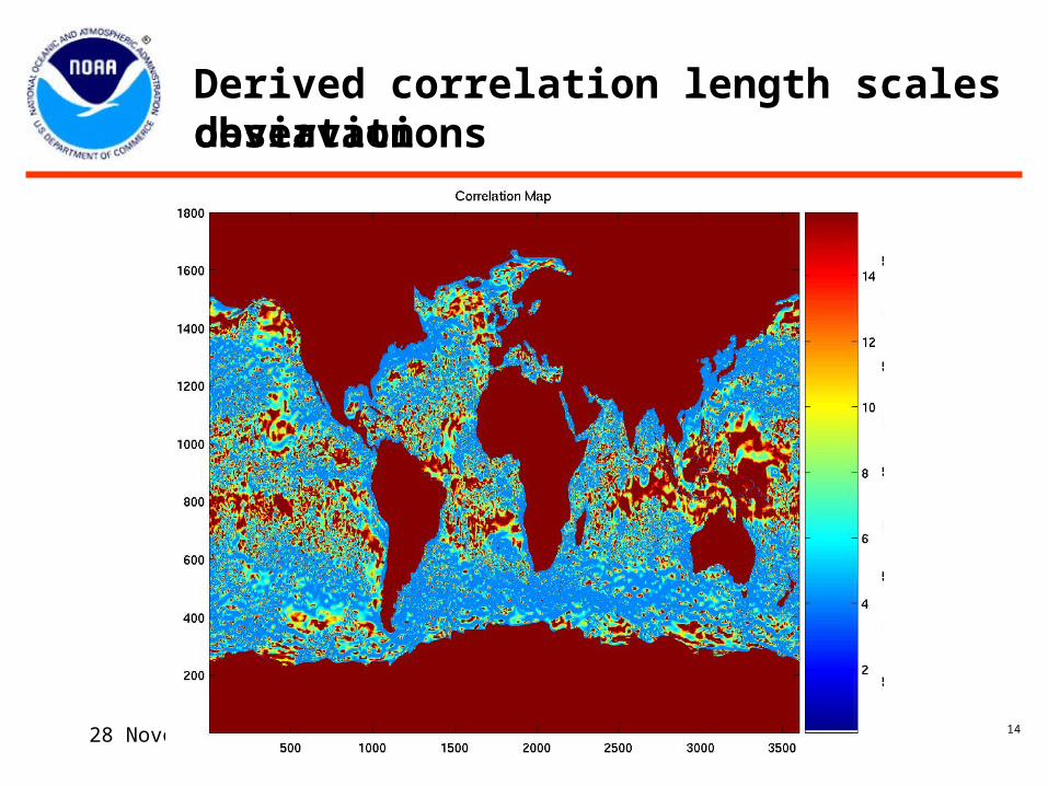
Correlation Map

• Variability of the SST field – Gulf of Mexico-short length scale (distance from data interpolation for sst

determination)– Southern Pacific-long length scale

• Spatial Variability of measurements DATA DRIVEN (daily)

– low variability-appropriate to use long length scales• lots of data than do not want to use a long length scale (cause smoothing)

(this allows us to preserve fine scales features)– lot of variability, good data coverage, use short length scales

• Three fixed correlation length scales( fixed in software covers range)– Generate 3 stationary maps of SST anomaly– interpolate between these to get our SST anomaly map that matches the

correlation map– Add the new SST anomaly to the previous day SST analysis

28 November 2006 MISST Meeting Washington, D.C. 14

One day of bias-corrected observationsEstimated daily absolute deviationDerived correlation length scales

28 November 2006 MISST Meeting Washington, D.C. 15

VALIDATION

• Evaluated against the RTG_SST ½°×½° resolution (also planning validation against 1/12°×1/12°) operational NCEP product

• Traditional in situ data e.g. buoys

28 November 2006 MISST Meeting Washington, D.C. 16

POES/GOES SSTRegional Analysis-East Coast

Click on image toplay

28 November 2006 MISST Meeting Washington, D.C. 17

Tropical Instability WavesDepicted by SST Analysis

Click on image toplay

28 November 2006 MISST Meeting Washington, D.C. 18

Validation vs. RTG Analysis & TMI

28 November 2006 MISST Meeting Washington, D.C. 19

More RTG & TMI comparisons

28 November 2006 MISST Meeting Washington, D.C. 20

Comparisons in Baja, CA

28 November 2006 MISST Meeting Washington, D.C. 22

METEOSAT-8 SSTs

• Meteosat-8 SST planned to be generated by NOAA/NESDIS February 2007

• Will be included in Multi-SST Analysis after errors are characterized

28 November 2006 MISST Meeting Washington, D.C. 23

MTSAT-1R

• SST product covering the Western Pacific and Eastern Indian Ocean to be developed from MTSAT-1R data by June 2007

• Will be included in Multi-SST Analysis after viable SST product is available and errors have been characterized

MULTI-SST ANALYSIS

WEB SITE: http://www.orbit.nesdis.noaa.gov/sod/sst/blended_sst

28 November 2006 MISST Meeting Washington, D.C. 26

SUMMARY

• NESDIS’ new SST analysis is:– Due to become an operational product (the ‘way

forward’, e.g. CoastWatch→OceanWatch)– Will benefit from improved pre-processing based

on MISST-derived knowledge– Is an ideal tool/test-bed for ascertaining the

benefits of the products and techniques being developed within MISST