eindhoven university of technology master bending … · of an axial force on the bending moment...
TRANSCRIPT

Eindhoven University of Technology
MASTER
Bending-normal force interaction of I-shaped cross-sections
experimental, numerical and statistical evaluation of the effect of an axial force on thebending moment resistance (bending and normal force interaction) of doublysymmetrical I-shaped cross-sections : part B : experimental, numerical and statisticalinvestigation
Rombouts, I.M.J.
Award date:2015
DisclaimerThis document contains a student thesis (bachelor's or master's), as authored by a student at Eindhoven University of Technology. Studenttheses are made available in the TU/e repository upon obtaining the required degree. The grade received is not published on the documentas presented in the repository. The required complexity or quality of research of student theses may vary by program, and the requiredminimum study period may vary in duration.
General rightsCopyright and moral rights for the publications made accessible in the public portal are retained by the authors and/or other copyright ownersand it is a condition of accessing publications that users recognise and abide by the legal requirements associated with these rights.
• Users may download and print one copy of any publication from the public portal for the purpose of private study or research. • You may not further distribute the material or use it for any profit-making activity or commercial gain
Take down policyIf you believe that this document breaches copyright please contact us providing details, and we will remove access to the work immediatelyand investigate your claim.
Download date: 08. Jun. 2018

Department of the Built Environment Structural Design
Den Dolech 2, 5612 AZ Eindhoven P.O. Box 513, 5600 MB Eindhoven The Netherlands www.tue.nl
Author
I.M.J. (Iris) Rombouts Boschdijk 339 5621 JA Eindhoven 06-46786213 0717121
Supervisors
prof.ir. H.H. (Bert) Snijder ir. R.W.A. (Rianne) Dekker dr.ir. P.A. (Paul) Teeuwen
Date
December 2014
Our reference
A/O-2014.80
Bending-Normal Force Interaction of I-shaped cross-sections
Experimental, numerical and statistical evaluation of the effect of an axial force on the bending moment resistance (bending and normal force interaction) of doubly symmetrical I-shaped cross-sections
Part B: experimental, numerical and statistical investigation
22/01/2015 Bending-normal force interaction of I-shaped cross-sections | I.M.J. Rombouts| 2

22/01/2015 Bending-normal force interaction of I-shaped cross-sections | I.M.J. Rombouts| 3
ACKNOWLEDGEMENTS
In this report I present my graduation project about the assessment of the cross-sectional design rules regarding I-shaped cross-sections in steel subjected to combined bending and normal force. The project process is supervised by prof.ir. H.H. (Bert) Snijder, Professor of Steel Structures at Eindhoven University of Technology (TU/e); ir. R.W.A. (Rianne) Dekker, TU/e doctoral candidate (PhD) for the assessment of cross-sectional design rules regarding the ductile failure modes and dr.ir. P.A. (Paul) Teeuwen, structural engineer at Witteveen+Bos. First of all I would like to thank my supervisors for sharing their knowledge, experience and enthusiasm. I want to thank H.H. (Bert) Snijder for giving me the opportunity to join the SAFEBRICTILE meeting to present my research results.
I also would like to thank the staff of the Pieter van Musschenbroek Laboratory at Eindhoven University of Technology, especially Theo van de Loo and Eric Wijen for helping me with the experimental tests. Iris Rombouts Eindhoven, December 2014

22/01/2015 Bending-normal force interaction of I-shaped cross-sections | I.M.J. Rombouts| 4
SUMMARY This research project, as part of work package 3 of the SAFEBRICTILE project, focuses on the resistance of a cross-section subjected to combined (uni-axial) bending and normal force (M-N interaction). The aim of this research project is:
assessment of the cross-sectional design rules regarding M-N interaction by means of an experimental, numerical and statistical evaluation of the effect of an axial force on the plastic bending moment resistance of doubly symmetrical I-shaped cross-sections in steel.
The Eurocode design rules [1], which are mostly based on mechanics, show unsafe approximations of the reduced plastic moment capacity for M-N interaction compared to the exact solution. Besides this, the partial factor which has to be used is γM0 = 1.00 and relative large shear forces are allowed, which means that there is no spare capacity available. Together with the fact that cross-sections subjected to multiple internal forces could react differently than predicted by theory it is clear that a reassessment of the design rules is necessary to ensure safety. Numerical tests results obtained with a numerical model validated with a few experimental tests will show if the design rules and/or partial safety factor are correct for My-N interaction. The force-deformation curves of the full-scale My-N interaction tests all showed a distinct elastic branch followed by a decreasing plastic branch, caused by the small extra moment due to increasing eccentricity. The specimens were not able to reach the state of strain hardening, since the cross-sections are largely loaded by compression and the flanges/web started to ‘buckle’ after yielding before strain hardening was reached. Comparing the experimental test results with Eurocode design rules, these rules seems to be safe when the nominal or characterizing measured yield strength is used for the entire cross-section, which is mostly the case. In this research project, the material behaviour over the cross-section is investigated in detail, resulting in accurate Eurocode design predictions for the experiments with high normal forces and unsafe predictions for cases with a small normal force and high bending moment. To get a better insight in the comparison between the design rules and actual material behaviour, Finite Element (FE) simulations are performed with a model that is validated against the experimental test results. The numerical results showed accurate estimations for the exact solution method, while the Eurocode [1] is unsafe for the combination of a small normal force and a high bending moment. The reduced bending moment capacity is majorly influenced by the ratio of the area of the web over the total area of the cross-section. Since the nominal numerical results are not only be discounted for the error of the resistance function, but also for the favourable distribution of the main variables (for example yield stress), the partial safety factor used in the Eurocode [1] design rules is statistically acceptable. Moreover, these distributions are constantly improving, mainly leading to a decrease of the partial safety factor. The main conclusion of this research project is stated as:
the behaviour of a cross-section with slender flanges subjected to combined strong axis bending and normal force is similar to the theoretical exact behaviour. The partial safety factor used in the Eurocode design rules for My-N interaction is statistically acceptable for these cross-sections with steel grades S235, S355 and S460.

22/01/2015 Bending-normal force interaction of I-shaped cross-sections | I.M.J. Rombouts| 5
SAMENVATTING Dit onderzoeksproject, dat deel uitmaakt van work package 3 van het SAFEBRICTILE project, focust op de weerstand van een doorsnede onderworpen aan de combinatie van een-assige buiging en normaalkracht (M-N interactie). Het doel van dit onderzoeksproject is:
beoordelen van de ontwerpregels omtrent M-N interactie door middel van experimenteel, numeriek en statistisch onderzoek naar het effect van een axiale kracht op de plastisch buigend moment capaciteit van dubbelsymetrische I-vormige doorsnedes in staal.
De ontwerpregels in de Eurocode [1], welke vooral zijn gebaseerd op mechanica, tonen onveilige inschattingen voor de gereduceerde plastische moment capaciteit voor M-N interactie vergeleken met de exacte oplossing. Daarnaast is de partiële veiligheidsfactor γM0 = 1.00 en vrij hoge dwarskrachten worden tegelijkertijd toegestaan. Dit betekent dat er weinig reservecapaciteit over is in de doorsnede. Samen met het feit dat een doorsnede onderworpen aan een combinatie van snedekrachten zich anders kan gedragen dan de theorie het voorschrijft, is het duidelijk dat een herwaardering van de ontwerpregels nodig is om onveilige situaties te voorkomen. Numerieke test resultaten verkregen met een numeriek model gevalideerd aan een aantal experimentele testen zullen uitwijzen of de ontwerpregels en/of partiele veiligheidsfactor correct zijn voor My-N interactie. De kracht-verplaatsings diagrammen van de volle schaal My-N interactie proeven toonden allemaal een duidelijke elastische tak, gevolgd door een afnemende plastische tak, veroorzaakt door het kleine extra moment dankzij de toenemende excentriciteit. De doorsneden waren niet in staat om de versteviging te bereiken, omdat de flenzen en/of het lijf gingen plooien door het vloeien dankzij de grote drukkrachten, voordat de staat van versteviging kon worden bereikt. Als de proefresultaten worden vergeleken met de ontwerpregels in de Eurocode [1] lijken ze veilig, wanneer de nominale of de karakteristieke vloeigrens wordt ingevuld voor het gehele profiel wat meestal ook het geval is. Echter, voor dit onderzoeksproject is het materiaalgedrag meer nauwkeurig onderzocht, resulterend in nauwkeurige Eurocode [1] voorspellingen voor de proeven met hoge normaalkrachten en onveilige resultaten voor de proeven met lage normaalkrachten gecombineerd met een groot buigend moment. Om meer inzicht te krijgen in de vergelijking tussen de ontwerpregels en de realiteit zijn numerieke simulaties uitgevoerd met een model dat is gevalideerd aan de experimentele test resultaten. De numerieke testen toonden dat de exacte oplossing nauwkeurige voorspellingen genereert, terwijl de Eurocode [1] onveilige resultaten geeft voor kleine normaalkrachten gecombineerd met veel buiging. De invloedrijkste factor is de ratio van het lijfoppervlak over het totale oppervlak van de doorsnede. Omdat de nominale numerieke testen niet alleen worden verdisconteerd naar de afwijking in de ontwerpregel, maar ook voor de (gunstige) statistische verdelingen van de hoofdvariabelen, is de partiële veiligheidsfactor zoals gebruikt in de Eurocode [1] statistisch gezien acceptabel. Daarnaast zijn de verdelingen van deze variabelen constant onderworpen aan veranderingen en zullen worden verbeterd. Gelukkig lijkt het erop dat met name de verdeling van de vloeigrens alleen maar gunstiger wordt, wat leidt tot een daling van de partiële veiligheidsfactor. De hoofdconclusie van dit onderzoeksproject is als volgt:
het gedrag van een doorsnede met slanke flenzen onderworpen aan een combinatie van buiging om de sterke as en normaalkracht is soortgelijk aan het theoretische exacte gedrag. De partiële veiligheidsfactor zoals gebruikt in de ontwerpregels in de Eurocode [1] voor My-N interactie is statistisch gezien acceptabel voor deze doorsneden in S235, S355 en S460.

22/01/2015 Bending-normal force interaction of I-shaped cross-sections | I.M.J. Rombouts| 6
TABLE OF CONTENTS
ACKNOWLEDGEMENTS ........................................................................................................................................ 3
SUMMARY ................................................................................................................................................................. 4
SAMENVATTING ..................................................................................................................................................... 5
1. INTRODUCTION ........................................................................................................................................ 11
1.1 Scope ................................................................................................................................................. 11
2. LITERATURE SURVEY ............................................................................................................................. 12
2.1 Cross-sectional resistance................................................................................................................. 12
2.2 Theoretical reference calculation ..................................................................................................... 13
2.3 Code requirements ........................................................................................................................... 14
2.4 Background documentation of the Eurocode .................................................................................. 15
2.5 Recent proposals for design rules..................................................................................................... 15
2.6 Results from earlier researches ........................................................................................................ 17
2.7 Conclusions and recommendations .................................................................................................. 17
3. EXPERIMENTS ........................................................................................................................................... 19
3.1 Motivation and objective .................................................................................................................. 19
3.2 Small scale experiments ................................................................................................................... 19
3.2.1 Tensile tests ........................................................................................................................................... 19
3.2.2 Compression tests ................................................................................................................................. 21
3.2.3 Stub column test ................................................................................................................................... 23
3.3 Full scale experiments ...................................................................................................................... 24
3.3.1 Experimental program ........................................................................................................................... 24
3.3.2 Loading .................................................................................................................................................. 25
3.3.3 Specimens ............................................................................................................................................. 27
3.3.4 Design of the test set-up ....................................................................................................................... 28
3.3.5 Specimen preparations ......................................................................................................................... 29
3.3.6 Measurements for the system response ............................................................................................... 30
3.3.7 Test results ............................................................................................................................................ 30
3.4 Summary, discussion and conclusions .............................................................................................. 41
3.4.1 Summary ............................................................................................................................................... 41
3.4.2 Discussion and conclusions ................................................................................................................... 44
4. FINITE ELEMENT SIMULATIONS ......................................................................................................... 48
4.1 Motivation and objective .................................................................................................................. 48
4.2 Simplifications ................................................................................................................................... 48

22/01/2015 Bending-normal force interaction of I-shaped cross-sections | I.M.J. Rombouts| 7
4.3 Pre-processing .................................................................................................................................. 48
4.3.1 Python script ......................................................................................................................................... 48
4.3.2 Geometry .............................................................................................................................................. 48
4.3.3 Elements ................................................................................................................................................ 49
4.3.4 Material ................................................................................................................................................. 49
4.3.5 Boundary conditions ............................................................................................................................. 51
4.3.6 Loading .................................................................................................................................................. 52
4.3.7 Mesh ...................................................................................................................................................... 52
4.4 Solving ............................................................................................................................................... 55
4.5 Post-processing ................................................................................................................................. 55
4.6 Validation of the FEM model ............................................................................................................ 55
4.6.1 Specimens MN0411/MN0412 ............................................................................................................... 57
4.6.2 Specimens MN0421/MN0422 ............................................................................................................... 58
4.6.3 Specimens MN0431/MN0432 ............................................................................................................... 59
4.6.4 Specimens MN0111/MN0112 ............................................................................................................... 60
4.6.5 Specimens MN0611/MN0612 ............................................................................................................... 61
4.6.6 Strain gauge validation .......................................................................................................................... 61
4.7 Summary, discussion and conclusions .............................................................................................. 62
4.7.1 Summary ............................................................................................................................................... 62
4.7.2 Discussion and conclusions ................................................................................................................... 64
5. PARAMETRIC STUDY .............................................................................................................................. 65
5.1 Resistance function and parameters ................................................................................................ 65
5.2 Sub-sets ............................................................................................................................................. 66
5.3 Numerical test results ....................................................................................................................... 70
5.4 Summary, discussion and conclusions .............................................................................................. 71
5.4.1 Summary ............................................................................................................................................... 71
5.4.2 Discussion and conclusions ................................................................................................................... 72
6. STATISTICAL EVALUATION .................................................................................................................. 73
6.1 Methodology .................................................................................................................................... 73
6.2 Statistical results ............................................................................................................................... 75
6.2.1 Cross-sections ........................................................................................................................................ 75
6.2.2 Utilization ratio’s ................................................................................................................................... 76
6.2.3 Steel grades ........................................................................................................................................... 76
6.2.4 Overall ................................................................................................................................................... 78
6.2.5 Coefficient of variation of the error term for the FEM model (Vδ,FEM) .................................................. 78
6.3 Summary, discussion and conclusions .............................................................................................. 79
6.3.1 Summary ............................................................................................................................................... 79
6.3.2 Discussion and conclusions ................................................................................................................... 80
7. BRIEF ADDITIONAL STUDIES .............................................................................................................. 82
7.1 Strain-hardening ............................................................................................................................... 82
22/01/2015 Bending-normal force interaction of I-shaped cross-sections | I.M.J. Rombouts| 8
7.2 Mz-N interaction ............................................................................................................................... 86
7.3 Tension as normal force ................................................................................................................... 87
8. CONCLUSIONS AND RECOMMENDATIONS ...................................................................................... 89
8.1 Conclusions ....................................................................................................................................... 89
8.2 Recommendations ............................................................................................................................ 90
9. REFERENCES .............................................................................................................................................. 93
10. ANNEXES ..................................................................................................................................................... 98
10.1 Positions of the tensile coupons .................................................................................................. 98
10.2 Results of the tensile coupons ................................................................................................... 100
10.3 Stress-strain curves in compression .......................................................................................... 115
10.4 Stub column test data ................................................................................................................ 116
10.5 Stress-strain curves in compression and tension ...................................................................... 118
10.6 Weighted stress-strain diagrams ............................................................................................... 119
10.7 Actual dimensions of the specimens ......................................................................................... 121
10.8 Test set-up ................................................................................................................................. 122
10.9 Test results MN0411 .................................................................................................................. 124
10.10 Test results MN0412 .................................................................................................................. 127
10.11 Test results MN0421 .................................................................................................................. 130
10.12 Test results MN0422 .................................................................................................................. 132
10.13 Test results MN0431 .................................................................................................................. 134
10.14 Test results MN0432 .................................................................................................................. 137
10.15 Test results MN0111 .................................................................................................................. 140
10.16 Test results MN0112 .................................................................................................................. 142
10.17 Test results MN0611 .................................................................................................................. 144
10.18 Test results MN0612 .................................................................................................................. 147
10.19 FEM model Python script ........................................................................................................... 150
10.20 Strain gauge validation .............................................................................................................. 163
10.21 Flow chart for the determination of Vrt ..................................................................................... 165
10.22 Statistical evaluation .................................................................................................................. 166
Digital Annex: CD with photos, movies and digital information
22/01/2015 Bending-normal force interaction of I-shaped cross-sections | I.M.J. Rombouts| 9
SYMBOLS
The list below gives an explanation of the symbols used in this report. Each symbol is explained when it is first mentioned in the text. a ratio between area of the web and total area of a cross-section = (A – 2 ∙ b ∙ tf) / A ≤ 0.5 - A area of a cross-section mm
2
b width of a cross-section mm b correction factor - E modulus of elasticity N/mm
2
fy yield strength N/mm2
h depth of a cross-section kd design fractile factor = 3.04 - m My,Ed / My,pl,Rd - MEd design bending moment kNm MN,Rd reduced design value of the resistance to bending moments about one principal axis
making allowance for the presence of normal forces kNm
Mpl,Rd plastic design resistance for bending about one principal axis of a cross-section kNm n utilization ratio = NEd / Npl,Rd - n number of numerical tests - NEd design value of the axial force kN Npl,Rd design plastic resistance to normal forces of the gross cross-section kN NRd design value of the resistance to normal forces kN r root radius mm re experimental (numerical in this case) resistance kNm rt theoretical resistance kNm s∆ standard deviation of ∆ - tf thickness of the flange Mm tw thickness of the web mm Vδ coefficient of variation of the error team - Vrt coefficient of variation of the basic input variables - Wpl plastic section modulus mm
3
β reliability index - σ standard deviation - δ error term - ∆ Logarithm of the error term - σtrue true stress N/mm
2
σnom Engineering stress N/mm2
εtrue True strain - εnom Engineering strain -
εpl True plastic strain -
γM partial factor for resistance of cross-sections - c.o.v. coefficient of variation, calculated by standard deviation / mean value %

22/01/2015 Bending-normal force interaction of I-shaped cross-sections | I.M.J. Rombouts| 10

22/01/2015 Bending-normal force interaction of I-shaped cross-sections | I.M.J. Rombouts| 11
1. INTRODUCTION
The built environment requires guaranteed structural safety, ensured by structural design rules. For steel structures, the cross-sectional resistance of all individual members, the strength of the connections and the structural stability of the complete steel structure needs to be evaluated. To provide a common approach for the design of structures all members of the European Union make use of the EN Eurocodes from 2012. The “EN 1993-1-1: Design of steel structures” [1] is used to solve issues in the built environment regarding the structural material steel with a certain level of safety. It is constantly subjected to changes to stay up to date since many changes have taken place after the first draft of the Eurocode [1]. For instance the use of higher steel grades has become more common in building practice. The background of the design rules for the cross-sectional resistance of members is limited, old-fashioned and/or purely based on mechanics. This mechanic approach is reliable for cross-sections subjected to single internal forces, but the interaction of multiple internal forces might be less straightforward. These cross-sections could react differently than predicted by the theory and therefore reassessment of these design rules is necessary to ensure safety This research project, as part of work package 3 of the SAFEBRICTILE project, focuses on the resistance of a cross-section subjected to combined (uni-axial) bending and axial force (M-N interaction). The aim of this research project is:
assessment of the cross-sectional design rules regarding M-N interaction by means of an experimental, numerical and statistical evaluation of the effect of an axial force on the plastic bending moment resistance of doubly symmetrical I-shaped cross-sections in steel.
This report is the second part of the research project on M-N interaction of I-shaped cross-sections. The first part of the investigation, indicated as Part A: literature survey [27], is briefly described in this report. This second part is focussed on the description of the experimental, numerical and statistical research. This report will start with a summary of the literature survey (part A). Thereafter the complete experimental program is described, divided into small scale experiments and full scale experiments. This is followed by the elaboration of the Finite Element simulations, which are validated against the experimental test results. This Finite Element Model is used to create a population of numerical tests for the parametric study and statistical evaluation, which is explained in chapter 5 and 6. The statistical evaluation will show whether the governing design rules match the actual behaviour, a modified design rule or value for the partial factor (γM) is more suitable. This report ends with the description of four limited additional investigations with regard to M-N interaction, followed by the main conclusions and recommendations.
1.1 Scope The scope of the cross sectional design rules regarding M-N interaction described by the Eurocode [1] is limited to article 6.2.9.1. Only I-shaped, H-shaped, rectangular solid and hollow cross-sections of steel quality S235, S355 and S460 are regarded. In the future this article will include other kind of cross-sections and higher steel strengths. The research project displays results of I- and H-shaped sections which show plastic behaviour without interference of stability issues like local buckling. This means that the cross-section has to reach the plastic moment, and therefore yielding of the complete cross-section has to occur. Torsion is not covered in this investigation, because it is considered to be out of scope.

22/01/2015 Bending-normal force interaction of I-shaped cross-sections | I.M.J. Rombouts| 12
2. LITERATURE SURVEY
This chapter contains the summary of the first part of the research on M-N interaction of I-shaped cross-sections. For an extended description of the literature survey, see Part A: literature survey [27].
2.1 Cross-sectional resistance Most design is performed on elastic behaviour of a structure, however a structure which is made of steel can bear some local yielding and will not actually collapse until sufficient ‘plastic hinges’ have formed. A ‘plastic hinge’ is a point in the structure were the cross-section is fully yielded, so that it is behaving in a plastic way and it will continue to deform without any increase in the moment until the state of strain hardening occurs. Since not every cross-section is able to reach this plastic behaviour, the capacity of a cross-section can be determined by two different theories: the elastic and plastic theory, which depends on the geometry of a cross-section. The difference between both stress distributions is indicated in Figure 2.1. When the bending moment is build up from zero, an elastic stress distribution occurs (Figure 2.1a). By increasing the moment a bit more the stress in the ultimate fibre reaches the yield stress (Figure 2.1b), but the stress distribution remains elastic. In the case that the moment is increased even further, more and more fibres starts to yield which is stated as ‘elasto-plastic’ behaviour (Figure 2.1c). Hereafter, the entire cross-section yields and plastic behaviour is reached (Figure 2.1d), which means that plastic hinges with such a rotation capacity that the moments can redistribute. Finally some cross-sections are able to reach the state of strain hardening (Figure 2.1e). At that moment the strength of the material is increased, while ductility decreased due to interacting dislocations (microscopic defects), which form a new internal structure.
Figure 2.1 Stress distributions (left) and corresponding idealized stress-strain relationship (right) [2]
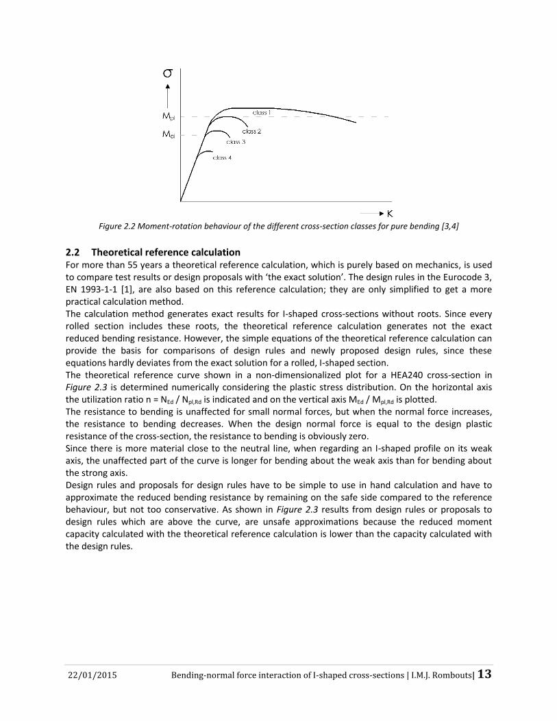
Figure 2.2 illustrates the difference in moment-rotation behaviour of a column subjected to a bending moment for compact, non compact and plastic sections. The class 1 cross-sections exceed the plastic moment capacity because of strain hardening. For class 1 and 2 the plastic theory can be used for the calculation of the resistance of the section. Calculations for class 3 and 4 cross-sections have to be based on elastic material behaviour, where in case of a class 4 cross-section even a local buckling calculation is required. Since this research project focuses on the plastic behaviour of cross-sections, it considers cross-sections which are categorized as class 1 and 2 sections.
22/01/2015 Bending-normal force interaction of I-shaped cross-sections | I.M.J. Rombouts| 13
Figure 2.2 Moment-rotation behaviour of the different cross-section classes for pure bending [3,4]
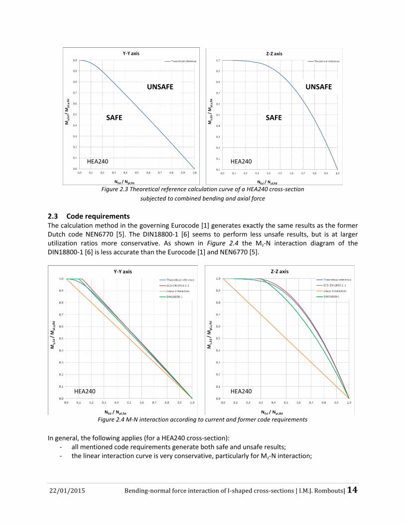
2.2 Theoretical reference calculation For more than 55 years a theoretical reference calculation, which is purely based on mechanics, is used to compare test results or design proposals with ‘the exact solution’. The design rules in the Eurocode 3, EN 1993-1-1 [1], are also based on this reference calculation; they are only simplified to get a more practical calculation method. The calculation method generates exact results for I-shaped cross-sections without roots. Since every rolled section includes these roots, the theoretical reference calculation generates not the exact reduced bending resistance. However, the simple equations of the theoretical reference calculation can provide the basis for comparisons of design rules and newly proposed design rules, since these equations hardly deviates from the exact solution for a rolled, I-shaped section. The theoretical reference curve shown in a non-dimensionalized plot for a HEA240 cross-section in Figure 2.3 is determined numerically considering the plastic stress distribution. On the horizontal axis the utilization ratio n = NEd / Npl,Rd is indicated and on the vertical axis MEd / Mpl,Rd is plotted. The resistance to bending is unaffected for small normal forces, but when the normal force increases, the resistance to bending decreases. When the design normal force is equal to the design plastic resistance of the cross-section, the resistance to bending is obviously zero. Since there is more material close to the neutral line, when regarding an I-shaped profile on its weak axis, the unaffected part of the curve is longer for bending about the weak axis than for bending about the strong axis. Design rules and proposals for design rules have to be simple to use in hand calculation and have to approximate the reduced bending resistance by remaining on the safe side compared to the reference behaviour, but not too conservative. As shown in Figure 2.3 results from design rules or proposals to design rules which are above the curve, are unsafe approximations because the reduced moment capacity calculated with the theoretical reference calculation is lower than the capacity calculated with the design rules.
22/01/2015 Bending-normal force interaction of I-shaped cross-sections | I.M.J. Rombouts| 14
Figure 2.3 Theoretical reference calculation curve of a HEA240 cross-section
subjected to combined bending and axial force
2.3 Code requirements The calculation method in the governing Eurocode [1] generates exactly the same results as the former Dutch code NEN6770 [5]. The DIN18800-1 [6] seems to perform less unsafe results, but is at larger utilization ratios more conservative. As shown in Figure 2.4 the Mz-N interaction diagram of the DIN18800-1 [6] is less accurate than the Eurocode [1] and NEN6770 [5].
Figure 2.4 M-N interaction according to current and former code requirements
In general, the following applies (for a HEA240 cross-section):
- all mentioned code requirements generate both safe and unsafe results; - the linear interaction curve is very conservative, particularly for Mz-N interaction;
SAFE
UNSAFE
SAFE
UNSAFE
HEA240 HEA240
HEA240 HEA240

22/01/2015 Bending-normal force interaction of I-shaped cross-sections | I.M.J. Rombouts| 15
- the DIN18800-1 generates less unsafe results for MY-N interaction for values of n < 0.35 compared to the Eurocode and the NEN6670;
- the DIN18800-1 generates more conservative results for values of n > 0.35 compared to the Eurocode and the NEN6670 for Mz-N interaction.
2.4 Background documentation of the Eurocode The governing Eurocode 3 [1] design rules regarding bending and normal force interaction refer to tests from 40 years ago, which were originally performed to determine the cross-sectional classification limits. The background documentation supporting the design rules of the Eurocode [7] regarding M-N interaction consists of three experimental studies. One of the three investigations comprised useful test results. The seven results of the study performed by Perlynn and Kulak [8] are all safe compared to the reference calculation, as shown in Figure 2.5. This might be explained by strain hardening and makes the test results less valuable.
Figure 2.5 Test results by Perlynn and Kulak compared with the theoretical reference
2.5 Recent proposals for design rules The last few years a lot of proposals to section 6.2.9.1 in the Eurocode [1] are presented to make the governing codes more accurate and safe. The disadvantage of these proposals is that they are only based on mechanics (a theoretical reference calculation) and not validated by means of experiments or a numerical model. Figure 2.6 shows all curves of the proposals and design rules in one figure. It is not possible to indicate the best proposal for new design rules, while some proposals approximate better at high values than low values and vice versa. In general, the following applies (for a HEA240 cross-section):
- only the modified DIN 18800-1 generates just safe results; - only the proposal by Tebedge and Chen generates just unsafe results; - Lindner’s proposals and the proposal by Tebedge and Chen give less accurate results for low
values of n;

22/01/2015 Bending-normal force interaction of I-shaped cross-sections | I.M.J. Rombouts| 16
- particularly the proposals from Vilette, Höglund, Matthey and Duan and Chen are safe for low values of n.
Figure 2.6 My-N interaction of proposals and design rules
Figure 2.7 shows all curves of the proposals and design rules for Mz-N interaction in one figure. General conclusions for these proposals are:
- the modified DIN 18800-1 and the proposal from CTICM generate safe results only; - the proposals from CTICM, which is equal to the proposal for My-N interaction, show very
inaccurate results, with a maximum deviation of 56.6% from the theoretical reference.
Figure 2.7 Mz-N interaction of proposals and design rules
HEA240 HEA240
HEA240

22/01/2015 Bending-normal force interaction of I-shaped cross-sections | I.M.J. Rombouts| 17
2.6 Results from earlier researches The studies on M-N interaction are rather old, recent research is limited and focussed on My-N interaction. The most important study is the research of Hasham and Rasmussen [9]. They performed an extensive study to a geometric and material non-linear Finite Element Method (FEM) model at the University of Sydney to investigate slender I-sections in High Strength Steel (HSS) subjected to combined bending and normal force. Section capacities (local buckling and in-plane bending) as well as member capacities (overall instability) were investigated. To validate this model, four series of tests on welded full-scale slender I-sections from (HSS) grade 350 in combined compression and major axis bending were preformed. Two series were conducted to determine the My-N interaction curves concerning the section capacity of beam cross-sections (stocky flanges and slender web) and column type cross-section (slender flanges and web). By means of this FEM model, Hasham and Rasmussen performed a research on different cross-sections [10]. Two types of slender sections were tested numerically, one non-compact and one compact section. Test results showed that for a compact section there was no noticeable change in strength due to residual stresses, while for the slender section the strength certainly changed. In addition, the FEM model showed that the shape of the My-N interaction curve for the compact section is convex, just like predicted by all theories. Hasham and Rasmussen presented that the cross-section capacity is underestimated by the theoretical reference calculation, but they did not validated the FEM model by means of experiments on compact sections.
2.7 Conclusions and recommendations The major conclusions of the literature survey are briefly summarised as: - the theoretical reference calculation for M-N interaction shown in recent literature is not the exact
solution for rolled, I-shaped cross-sections. It gives a good approximation, since it consists of a more simple formula compared to exact solution and generates similar results;
- besides the fact that the Eurocode show unsafe approximations of the reduced plastic moment capacity for MY-N interaction for n < 0.45, the partial factor which has to be used is γM0 = 1.00 and relative large shear forces are allowed, which means that there is no spare capacity available;
- the linear interaction curve shown in the Eurocode [1] is very conservative, particularly for Mz-N interaction;
- for Mz-N interaction, the Eurocode generates unsafe results only; - the background documentation of the Eurocode design rules [7] contains seven useful test results
which are (very much) on the safe side, apparently benefitting from strain hardening; - a lot of new/modified proposals to section 6.2.9.1 in the Eurocode have been recently presented; - only the modified DIN 18800-1 generates just safe results for bending about the Y-Y- and Z-Z axis,
however the results for MZ-N interaction are conservative; - the modified DIN 18800-1 is a fair calculation method in terms of computational work for bending
about both axes; - experimental tests intended to investigate M-N interaction of compact sections were never
performed to the knowledge of the author. Only a small number of test results were generated for another purpose, but showed My-N interaction;
- Hasham and Rasmussen [10] showed that the theoretical reference calculation for My-N interaction underestimates the actual behaviour (generated by a FEM model) for compact sections. Unfortunately the Finite Element Model is only validated by means of experimental tests on slender cross-sections;
22/01/2015 Bending-normal force interaction of I-shaped cross-sections | I.M.J. Rombouts| 18
- Hasham and Rasmussen [10] also showed that the residual stresses have no significant influence on the plastic capacity of a cross-section.
The major recommendations for the continuation of the research project are: - experimental tests have to be performed on class 1 cross-sections to include and analyze the effect
of strain hardening in the FEM model, since it can be ‘turned off’ in the numerical model; - Mz-N interaction of compact sections is experimentally and numerically neglected in research (to
the knowledge of the author). Therefore, it is interesting to implement bending about the weak axis in the Finite Element Model in the final stage (when the model is able to accurately predict the actual behaviour for My-N interaction);
- the test set-up as used in the background documentation in the Eurocode [7] can be used as inspiration for the design of the test-set up used in this research project.
22/01/2015 Bending-normal force interaction of I-shaped cross-sections | I.M.J. Rombouts| 19
3. EXPERIMENTS
All experiments were carried out at the Pieter van Musschenbroek laboratory at Eindhoven University of Technology. Prior to the full scale experiments on My-N interaction small scale material tests have been carried out. The goal of these tests was to get information about the actual material behaviour under both compression and tension and thereby generate data about the material properties as input for the FEM model.
3.1 Motivation and objective Since there are almost no experimental test results available on M-N interaction, a new experimental test program had to be designed for the validation of the FEM model. A limited number of tests were performed, while the experiments are time consuming and expensive.
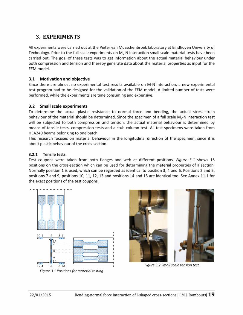
3.2 Small scale experiments To determine the actual plastic resistance to normal force and bending, the actual stress-strain behaviour of the material should be determined. Since the specimen of a full scale My-N interaction test will be subjected to both compression and tension, the actual material behaviour is determined by means of tensile tests, compression tests and a stub column test. All test specimens were taken from HEA240 beams belonging to one batch. This research focuses on material behaviour in the longitudinal direction of the specimen, since it is about plastic behaviour of the cross-section. 3.2.1 Tensile tests Test coupons were taken from both flanges and web at different positions. Figure 3.1 shows 15 positions on the cross-section which can be used for determining the material properties of a section. Normally position 1 is used, which can be regarded as identical to position 3, 4 and 6. Positions 2 and 5, positions 7 and 9, positions 10, 11, 12, 13 and positions 14 and 15 are identical too. See Annex 11.1 for the exact positions of the test coupons.
Figure 3.1 Positions for material testing
Figure 3.2 Small scale tension test

22/01/2015 Bending-normal force interaction of I-shaped cross-sections | I.M.J. Rombouts| 20
For the test coupons the static yield stress was measured to eliminate the influence of the speed of testing, the size of the specimen and the test rig, as Ziemian [11] showed. This is done by pausing the test rig three times in the yielding plateau and 3 times after yielding. At each stop the load drops until it stabilizes and creates low points in the stress–strain curve, as shown in Figure 3.3.
Figure 3.3 Stress-strain curves in tension, HEA240 (S235JR), coupon B2P8
The coupons were tensioned until rupture according to ISO 6892-1 [12] in a displacement controlled 250 kN test rig, as shown in Figure 3.2. The measured static and dynamic yield stresses are listed in Table 3.1. The stress-strain plots of the coupon tests are shown in Annex 11.2. Most of the stress-strain plots are similar, but the stress-strain behaviour on position 7 and 14 differs: the yield plateau cannot be defined and therefore the yield stress has to be calculated with the 0.2% proportional limit strain.
Table 3.1 Measured dynamic and static yield stresses in tension
Test coupon Static yield stress Dynamic yield stress Ratio Delta
Name Beam Position N/mm2 N/mm
2 % N/mm
2
B1P1 1 1 268 288 107.46% 20 B2P1 2 1 268 289 107.84% 21 B4P1 4 1 256 276 107.81% 20 B6P1 6 1 265 287 108.30% 22 B8P1 8 1 256 274 107.03% 18
Average 263 283 107.69% 20
B1P2 1 2 235 262 111.49% 27 B2P2 2 2 231 254 109.96% 23
Average 233 258 110.72% 25
B1P7 1 7 365 385 105.48% 20 B2P7 2 7 344 367 106.69% 23
Average 355 376 106.08% 22
B1P8 1 8 277 297 107.22% 20 B2P8 2 8 276 299 108.33% 23
Average 277 298 107.78% 22
22/01/2015 Bending-normal force interaction of I-shaped cross-sections | I.M.J. Rombouts| 21
T101 - 10 277 292 105.42% 20 T102 - 10 285 300 105.26% 15
Average 281 296 105.34% 18
T141 - 14 415 425 102.41% 10 T142 - 14 397 407 102.52% 10
Average 406 416 102.45% 10
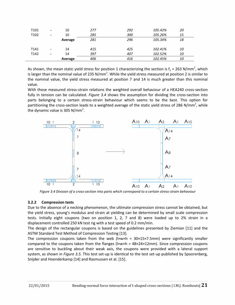
As shown, the mean static yield stress for position 1 characterizing the section is fy = 263 N/mm2, which is larger than the nominal value of 235 N/mm2. While the yield stress measured at position 2 is similar to the nominal value, the yield stress measured at position 7 and 14 is much greater than this nominal value. With these measured stress-strain relations the weighted overall behaviour of a HEA240 cross-section fully in tension can be calculated. Figure 3.4 shows the assumption for dividing the cross-section into parts belonging to a certain stress-strain behaviour which seems to be the best. This option for partitioning the cross-section leads to a weighted average of the static yield stress of 286 N/mm2, while the dynamic value is 305 N/mm2.
Figure 3.4 Division of a cross-section into parts which correspond to a certain stress-strain behaviour
3.2.2 Compression tests Due to the absence of a necking phenomenon, the ultimate compression stress cannot be obtained, but the yield stress, young’s modulus and strain at yielding can be determined by small scale compression tests. Initially eight coupons (two on position 1, 2, 7 and 8) were loaded up to 2% strain in a displacement controlled 250 kN test rig with a test speed of 0.2 mm/min. The design of the rectangular coupons is based on the guidelines presented by Ziemian [11] and the ASTM Standard Test Method of Compression Testing [13]. The compression coupons taken from the web (l×w×h = 30×15×7.5mm) were significantly smaller compared to the coupons taken from the flanges (l×w×h = 48×24×12mm). Since compression coupons are sensitive to buckling about their weak axis, the coupons were provided with a lateral support system, as shown in Figure 3.5. This test set-up is identical to the test set-up published by Spoorenberg, Snijder and Hoenderkamp [14] and Rasmussen et al. [15].
22/01/2015 Bending-normal force interaction of I-shaped cross-sections | I.M.J. Rombouts| 22
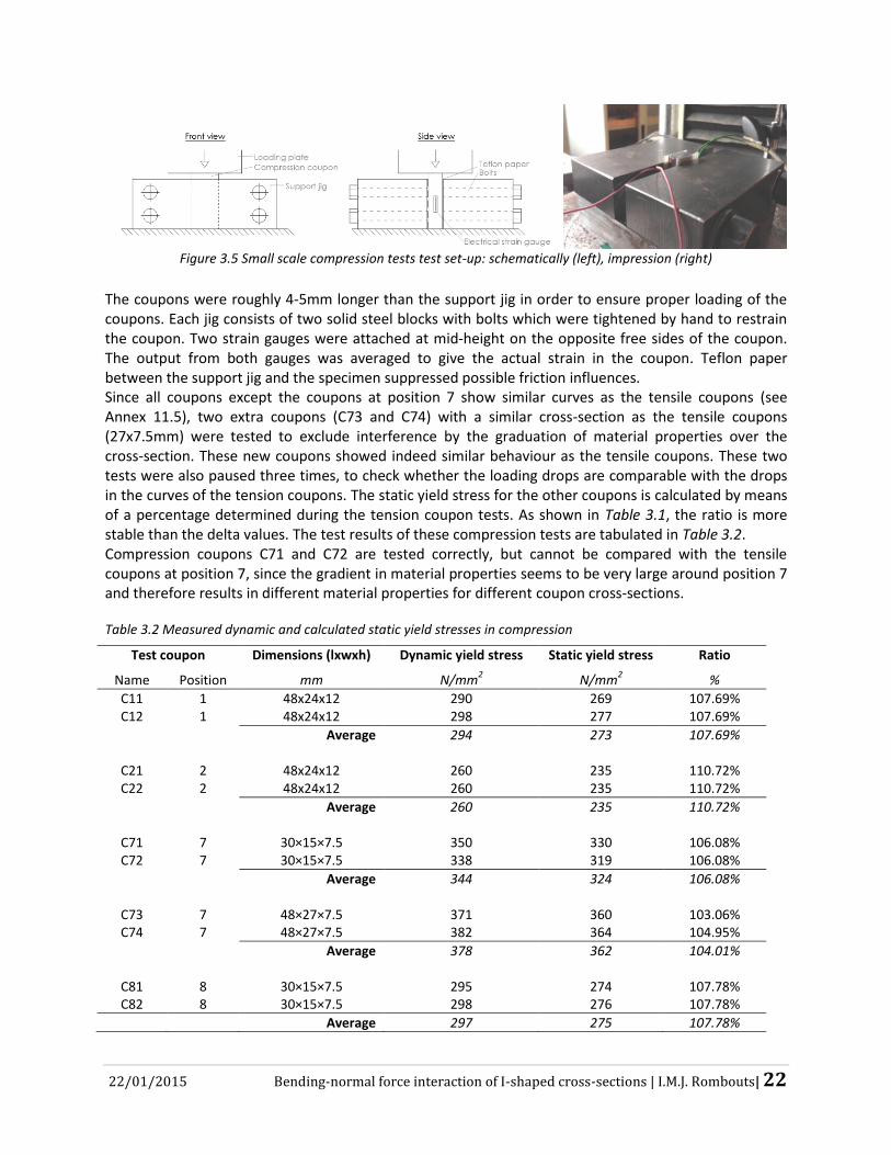
Figure 3.5 Small scale compression tests test set-up: schematically (left), impression (right)
The coupons were roughly 4-5mm longer than the support jig in order to ensure proper loading of the coupons. Each jig consists of two solid steel blocks with bolts which were tightened by hand to restrain the coupon. Two strain gauges were attached at mid-height on the opposite free sides of the coupon. The output from both gauges was averaged to give the actual strain in the coupon. Teflon paper between the support jig and the specimen suppressed possible friction influences. Since all coupons except the coupons at position 7 show similar curves as the tensile coupons (see Annex 11.5), two extra coupons (C73 and C74) with a similar cross-section as the tensile coupons (27x7.5mm) were tested to exclude interference by the graduation of material properties over the cross-section. These new coupons showed indeed similar behaviour as the tensile coupons. These two tests were also paused three times, to check whether the loading drops are comparable with the drops in the curves of the tension coupons. The static yield stress for the other coupons is calculated by means of a percentage determined during the tension coupon tests. As shown in Table 3.1, the ratio is more stable than the delta values. The test results of these compression tests are tabulated in Table 3.2. Compression coupons C71 and C72 are tested correctly, but cannot be compared with the tensile coupons at position 7, since the gradient in material properties seems to be very large around position 7 and therefore results in different material properties for different coupon cross-sections.
Table 3.2 Measured dynamic and calculated static yield stresses in compression
Test coupon Dimensions (lxwxh) Dynamic yield stress Static yield stress Ratio
Name Position mm N/mm2 N/mm
2 %
C11 1 48x24x12 290 269 107.69% C12 1 48x24x12 298 277 107.69%
Average 294 273 107.69%
C21 2 48x24x12 260 235 110.72% C22 2 48x24x12 260 235 110.72%
Average 260 235 110.72%
C71 7 30×15×7.5 350 330 106.08% C72 7 30×15×7.5 338 319 106.08%
Average 344 324 106.08%
C73 7 48×27×7.5 371 360 103.06% C74 7 48×27×7.5 382 364 104.95%
Average 378 362 104.01%
C81 8 30×15×7.5 295 274 107.78% C82 8 30×15×7.5 298 276 107.78%
Average 297 275 107.78%

22/01/2015 Bending-normal force interaction of I-shaped cross-sections | I.M.J. Rombouts| 23
Again, position 2 corresponds to the smallest yield stress and position 7 to the largest. The yield stress in compression at position 2 is equal to the nominal yield strength. A typical compression test result is shown in Figure 3.6, the others are displayed in Annex 11.3.
Figure 3.6 Stress-strain curve in compression, HEA240 (S235JR), coupon C21/C22
Annex 11.5 shows the comparison between tension and compression stress-strain curves at a similar position. The weighted global stress-strain behaviour under tension and compression calculated with the partition shown in Figure 3.4 is displayed in Annex 11.6. 3.2.3 Stub column test A stub column test was performed to determine the overall behaviour of a HEA240 cross-section in compression. The test performed according to Ziemian’s guidelines [11] consists of a specimen with a length of 500 mm which was compressed in a displacement controlled 2.5 MN actuator with a test speed of 0.3 mm/min until the load dropped significantly. Due to overall yielding the flanges started to ‘buckle’ in the end. Figure 3.7 shows an impression of the stub column test set-up.
Figure 3.7 Test set-up of the stub-column test
Four LVDT’s at the flange tips had to be used during alignment of the cross-section to check if the specimen was at equal height over de four flange tips. Two strain gauges at opposite position on the mid-height of the flanges were used to determine the stress-strain relationship of this stub column.
22/01/2015 Bending-normal force interaction of I-shaped cross-sections | I.M.J. Rombouts| 24
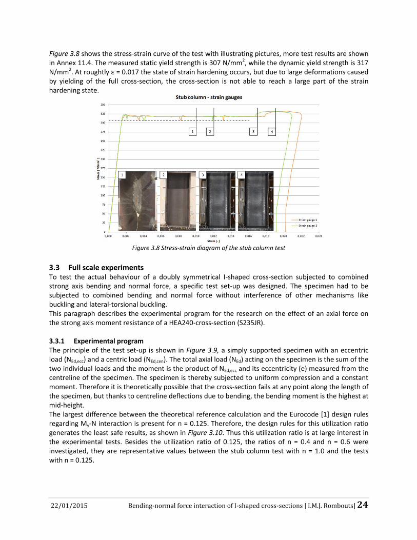
Figure 3.8 shows the stress-strain curve of the test with illustrating pictures, more test results are shown in Annex 11.4. The measured static yield strength is 307 N/mm2, while the dynamic yield strength is 317 N/mm2. At roughtly ε = 0.017 the state of strain hardening occurs, but due to large deformations caused by yielding of the full cross-section, the cross-section is not able to reach a large part of the strain hardening state.
Figure 3.8 Stress-strain diagram of the stub column test
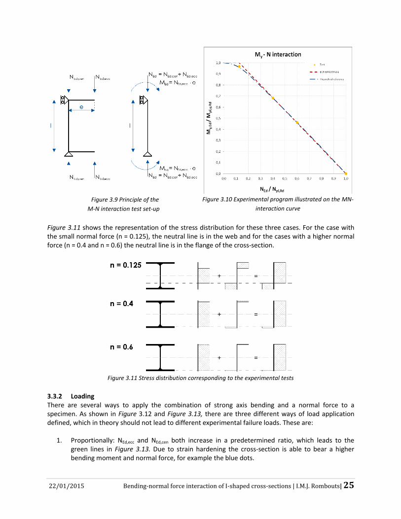
3.3 Full scale experiments To test the actual behaviour of a doubly symmetrical I-shaped cross-section subjected to combined strong axis bending and normal force, a specific test set-up was designed. The specimen had to be subjected to combined bending and normal force without interference of other mechanisms like buckling and lateral-torsional buckling. This paragraph describes the experimental program for the research on the effect of an axial force on the strong axis moment resistance of a HEA240-cross-section (S235JR). 3.3.1 Experimental program The principle of the test set-up is shown in Figure 3.9, a simply supported specimen with an eccentric load (NEd,ecc) and a centric load (NEd,cen). The total axial load (NEd) acting on the specimen is the sum of the two individual loads and the moment is the product of NEd,ecc and its eccentricity (e) measured from the centreline of the specimen. The specimen is thereby subjected to uniform compression and a constant moment. Therefore it is theoretically possible that the cross-section fails at any point along the length of the specimen, but thanks to centreline deflections due to bending, the bending moment is the highest at mid-height. The largest difference between the theoretical reference calculation and the Eurocode [1] design rules regarding My-N interaction is present for n = 0.125. Therefore, the design rules for this utilization ratio generates the least safe results, as shown in Figure 3.10. Thus this utilization ratio is at large interest in the experimental tests. Besides the utilization ratio of 0.125, the ratios of n = 0.4 and n = 0.6 were investigated, they are representative values between the stub column test with n = 1.0 and the tests with n = 0.125.
22/01/2015 Bending-normal force interaction of I-shaped cross-sections | I.M.J. Rombouts| 25
Figure 3.9 Principle of the
M-N interaction test set-up
Figure 3.10 Experimental program illustrated on the MN-
interaction curve
Figure 3.11 shows the representation of the stress distribution for these three cases. For the case with the small normal force (n = 0.125), the neutral line is in the web and for the cases with a higher normal force (n = 0.4 and n = 0.6) the neutral line is in the flange of the cross-section.
Figure 3.11 Stress distribution corresponding to the experimental tests
3.3.2 Loading There are several ways to apply the combination of strong axis bending and a normal force to a specimen. As shown in Figure 3.12 and Figure 3.13, there are three different ways of load application defined, which in theory should not lead to different experimental failure loads. These are:
1. Proportionally: NEd,ecc and NEd,cen both increase in a predetermined ratio, which leads to the green lines in Figure 3.13. Due to strain hardening the cross-section is able to bear a higher bending moment and normal force, for example the blue dots.

22/01/2015 Bending-normal force interaction of I-shaped cross-sections | I.M.J. Rombouts| 26
2. Constant moment (MEd): the moment which is adjusted from the proportional tests (at the blue dot in Figure 3.13) will be applied by NEd,ecc, thereafter NEd,cen will increase, creating the light blue lines in Figure 3.13.
3. Constant normal force (NEd): the normal force which is adjusted from the proportional test will be applied as NEd,cen. While NEd,ecc increases, NEd,cen decreases in such a way that NEd remains constant and MEd increases. The soft pink lines in Figure 3.13 represent the application method of the combined bending moment and normal force.
Figure 3.12 Manners of applying My-N interaction to the specimen (schematically)
Figure 3.13 Manners of applying My-N interaction to the specimen (graphically)
22/01/2015 Bending-normal force interaction of I-shaped cross-sections | I.M.J. Rombouts| 27
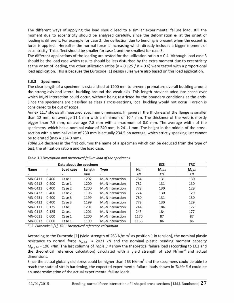
The different ways of applying the load should lead to a similar experimental failure load, still the moment due to eccentricity should be analyzed carefully, since the deformation e2 at the onset of loading is different. For example for case 2, the deflection due to bending is present when the eccentric force is applied. Hereafter the normal force is increasing which directly includes a bigger moment of eccentricity. This effect should be smaller for case 1 and the smallest for case 3. The different applications of the loading are tested for the utilization ratio n = 0.4. Although load case 3 should be the load case which results should be less disturbed by the extra moment due to eccentricity at the onset of loading, the other utilization ratios (n = 0.125 / n = 0.6) were tested with a proportional load application. This is because the Eurocode [1] design rules were also based on this load application. 3.3.3 Specimens The clear length of a specimen is established at 1200 mm to prevent premature overall buckling around the strong axis and lateral buckling around the weak axis. This length provides adequate space over which My-N interaction could occur, without being restricted by the boundary conditions at the ends. Since the specimens are classified as class 1 cross-sections, local buckling would not occur. Torsion is considered to be out of scope. Annex 11.7 shows all measured specimen dimensions. In general, the thickness of the flange is smaller than 12 mm, on average 11.1 mm with a minimum of 10.4 mm. The thickness of the web is mostly bigger than 7.5 mm, on average 7.8 mm with a maximum of 8.0 mm. The average width of the specimens, which has a nominal value of 240 mm, is 241.1 mm. The height in the middle of the cross-section with a nominal value of 230 mm is actually 234.5 on average, which strictly speaking just cannot be tolerated (max = 234.0 mm). Table 3.4 declares in the first columns the name of a specimen which can be deduced from the type of test, the utilization ratio n and the load case.
Table 3.3 Description and theoretical failure load of the specimens
Data about the specimen EC3 TRC
Name -
n -
Load case -
Length mm
Type -
NEd
kN My,Ed
kN My,Ed
kN
MN-0411 0.400 Case 1 1202 My-N interaction 784 131 130 MN-0412 0.400 Case 1 1200 My-N interaction 782 131 130 MN-0421 0.400 Case 2 1200 My-N interaction 778 130 129 MN-0422 0.400 Case 2 1196 My-N interaction 774 130 129 MN-0431 0.400 Case 3 1199 My-N interaction 780 131 130 MN-0432 0.400 Case 3 1199 My-N interaction 778 130 129 MN-0111 0.125 Case1 1201 My-N interaction 244 184 177 MN-0112 0.125 Case1 1201 My-N interaction 243 184 177 MN-0611 0.600 Case 1 1200 My-N interaction 1170 87 87 MN-0612 0.600 Case 1 1199 My-N interaction 1166 86 86
EC3: Eurocode 3 [1], TRC: Theoretical reference calculation
According to the Eurocode [1] (yield strength of 263 N/mm2 as position 1 in tension), the nominal plastic resistance to normal force Npl,Rd = 2021 kN and the nominal plastic bending moment capacity Mpl,y,Rd = 196 kNm. The last columns of Table 3.4 show the theoretical failure load (according to EC3 and the theoretical reference calculation) calculated with a yield strength of 263 N/mm2 and actual dimensions. Since the actual global yield stress could be higher than 263 N/mm2 and the specimens could be able to reach the state of strain hardening, the expected experimental failure loads shown in Table 3.4 could be an underestimation of the actual experimental failure loads.

22/01/2015 Bending-normal force interaction of I-shaped cross-sections | I.M.J. Rombouts| 28
3.3.4 Design of the test set-up Figure 3.14 and Figure 3.15 show an impression of the test set-up. The big frame is omitted in the schematic representation for clarity. Due to practical reasons the specimens were positioned in a vertical position. The introduction of the centric force was established by a 2 MN hydraulic jack. The eccentric force was introduced by a 1 MN hydraulic jack which tightens a tension rod (φ32 mm) at a distance of 750 mm from the centric force. The arms for applying the bending moment are made of HEM240 beams with stiffeners at 1/3 of its length. One stiffener is located at the centreline of the centric force, the other stiffener is located nearby the end of the specimen’s endplate. The endplates with a thickness of 30 mm are welded to the specimen and bolted with 8xM24 to the arms in which extra plates with t = 30 mm are bolted to increase the stiffness of the connection. A long plate with a thickness of t = 40 mm connects the eccentric jack with the arms. A triangular support with a hole ensures a stiff connection at the end of the arms. Due to four rockers (two underneath the jacks and two in the opposite position on the other arm) the specimen is free to bend to a maximum of 6⁰. The rockers permitted rotations about the weak axis of the specimen as well, but these rotations were negligible. All elements in the test set-up were checked on capacity and deformation to design a safe test environment. An extensive overview of the schematic representation of the test set-up is displayed in Annex 11.8.
Figure 3.14 Schematic representation of the My-N interaction test
set-up: beginning (left), deformed (right)

22/01/2015 Bending-normal force interaction of I-shaped cross-sections | I.M.J. Rombouts| 29
Figure 3.15 Impression of the My-N interaction test set-up
3.3.5 Specimen preparations Both the specimens and the end plates were smoothened with a metal grinder to remove the mill scale for a better welding process. The mill scale was also mechanically removed at locations were the electrical strain gauges had to be applied. Figure 3.16 show an overview of the specimens preparations: sawn columns (a), smoothened end plates (b), test set-up for welding (c), weld a = 5 mm (d), electrical strain gauges at the (smoothened places on the) mid-height of the cross-section (e).
(a) (b) (c)
(d) (e)
Figure 3.16 Specimen preparations
22/01/2015 Bending-normal force interaction of I-shaped cross-sections | I.M.J. Rombouts| 30
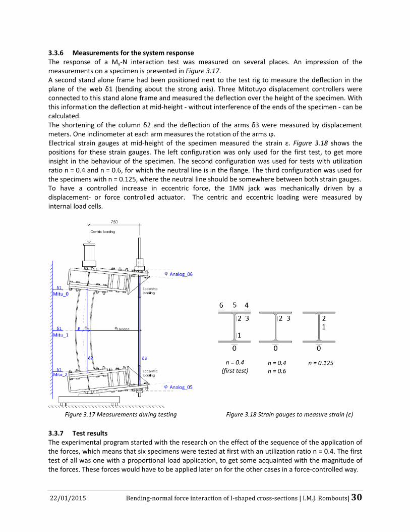
3.3.6 Measurements for the system response The response of a My-N interaction test was measured on several places. An impression of the measurements on a specimen is presented in Figure 3.17. A second stand alone frame had been positioned next to the test rig to measure the deflection in the plane of the web δ1 (bending about the strong axis). Three Mitotuyo displacement controllers were connected to this stand alone frame and measured the deflection over the height of the specimen. With this information the deflection at mid-height - without interference of the ends of the specimen - can be calculated. The shortening of the column δ2 and the deflection of the arms δ3 were measured by displacement meters. One inclinometer at each arm measures the rotation of the arms ϕ. Electrical strain gauges at mid-height of the specimen measured the strain ε. Figure 3.18 shows the positions for these strain gauges. The left configuration was only used for the first test, to get more insight in the behaviour of the specimen. The second configuration was used for tests with utilization ratio n = 0.4 and n = 0.6, for which the neutral line is in the flange. The third configuration was used for the specimens with n = 0.125, where the neutral line should be somewhere between both strain gauges. To have a controlled increase in eccentric force, the 1MN jack was mechanically driven by a displacement- or force controlled actuator. The centric and eccentric loading were measured by internal load cells.
Figure 3.17 Measurements during testing
Figure 3.18 Strain gauges to measure strain (ε)
3.3.7 Test results The experimental program started with the research on the effect of the sequence of the application of the forces, which means that six specimens were tested at first with an utilization ratio n = 0.4. The first test of all was one with a proportional load application, to get some acquainted with the magnitude of the forces. These forces would have to be applied later on for the other cases in a force-controlled way.
n = 0.4 (first test)
n = 0.4 n = 0.6
n = 0.125
22/01/2015 Bending-normal force interaction of I-shaped cross-sections | I.M.J. Rombouts| 31
For every set of two tests one specimen was continually loaded, the second was paused three times in the plastic curve to determine the static values of the test results. This paragraph shows force-deformation curves of all tests, in which the deformation e2 is the displacement at mid-height calculated for the fictitious case that the displacement at the top and bottom of the specimen are zero. Since Mitu_0 and Mitu_2 (see Figure 3.17) are placed at 60 mm from the top and bottom, at first the displacement at the bottom and top has to be calculated with a parabolic extrapolation to determine the actual e2, as shown in equation (3.1).
e2 = Mitu_1 -
Average(Mitu_0;Mitu_2) + (Mitu_1 - Average(Mitu_0;Mitu_2)) ∙
(5402 - 600
2)
5402 (3.1)
The force-deformation curves show both the eccentric and centric force plotted versus this deformation e2. The centric force is marked with a dark colour, while the eccentric force has a light colour of the same colour tone. Moreover, all test results are shown in detail in the Annex mentioned in the describing text. Overall, the experiments show a clearl elastic branch followed by a decreasing plastic branch, which might be caused by the small extra moment due to increasing eccentricity. Therefore, the utilization ratios are not stable during the tests, since the bending moment increases while the normal force decreases. The maximum force which is reached just after the start of the plastic branch is stated as the experimental ‘failure’ load. The total normal force NEd can be calculated by the sum of the two (centric and eccentric) maximum experimental failure loads, as shown in equation (3.2). To calculate the corresponding ‘failure’ moment My,Ed, equation (3.3) has to be used, in which Mitu_1 is used instead of e2, since Mitu_1 shows the actual eccentricity at mid-height.
NEd = Fexp,cen + Fexp,ecc (3.2)
My,Ed = Fexp,ecc ∙ (750 + Mitu_1) + Fexp,cen ∙ Mitu_1 (3.3)
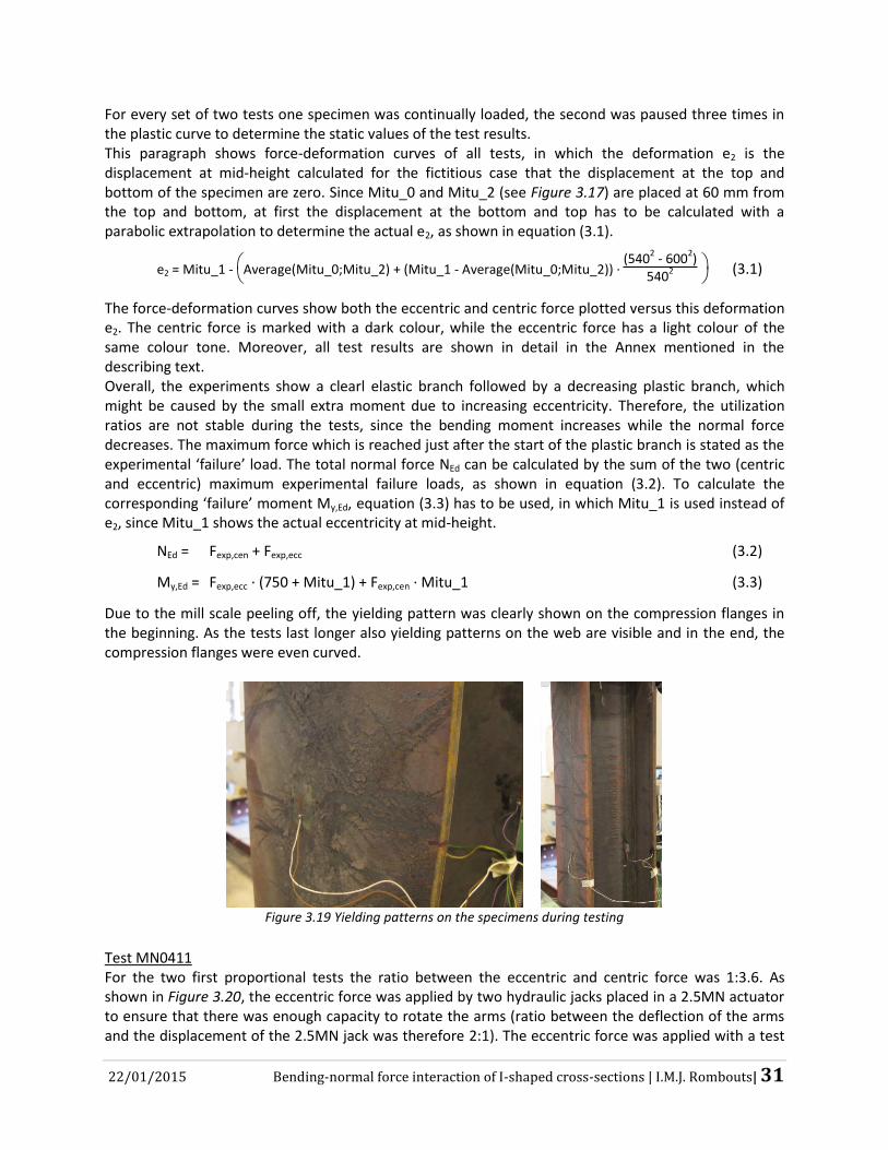
Due to the mill scale peeling off, the yielding pattern was clearly shown on the compression flanges in the beginning. As the tests last longer also yielding patterns on the web are visible and in the end, the compression flanges were even curved.
Figure 3.19 Yielding patterns on the specimens during testing
Test MN0411 For the two first proportional tests the ratio between the eccentric and centric force was 1:3.6. As shown in Figure 3.20, the eccentric force was applied by two hydraulic jacks placed in a 2.5MN actuator to ensure that there was enough capacity to rotate the arms (ratio between the deflection of the arms and the displacement of the 2.5MN jack was therefore 2:1). The eccentric force was applied with a test
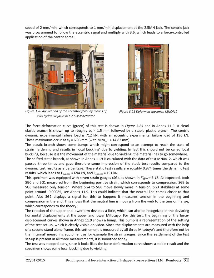
22/01/2015 Bending-normal force interaction of I-shaped cross-sections | I.M.J. Rombouts| 32
speed of 2 mm/min, which corresponds to 1 mm/min displacement at the 2.5MN jack. The centric jack was programmed to follow the eccentric signal and multiply with 3.6, which leads to a force-controlled application of the centric force.
Figure 3.20 Application of the eccentric force by means of
two hydraulic jacks in a 2.5 MN actuator
Figure 3.21 Deformed specimen MN0412
The force-deformation curve (green) of this test is shown in Figure 3.25 and in Annex 11.9. A clearl elastic branch is shown up to roughly e2 = 1.5 mm followed by a stable plastic branch. The centric dynamic experimental failure load is 712 kN, with an eccentric experimental failure load of 196 kN. These maximums occur at e2 = 6.06 mm (with Mitu_1 = 14.82 mm). The plastic branch shows some bumps which might correspond to an attempt to reach the state of strain hardening and results in ‘local buckling’ due to yielding. In fact this should not be called local buckling, because it is the movement of the material due to yielding: the material has to go somewhere. The shifted static branch, as shown in Annex 11.9 is calculated with the data of test MN0412, which was paused three times and gave therefore some impression of the static test results compared to the dynamic test results as a percentage. These static test results are roughly 0.974 times the dynamic test results, which leads to Fexp,cen = 694 kN, and Fexp,ecc = 191 kN. This specimen was equipped with seven strain gauges (SG), as shown in Figure 3.18. As expected, both SG0 and SG1 measured from the beginning positive strain, which corresponds to compression. SG3 to SG6 measured only tension. Where SG4 to SG6 move slowly more in tension, SG3 stabilizes at some point around -0.00085, see Annex 11.9. This could indicate that the neutral line comes closer to that point. Also SG2 displays a signal for this to happen: it measures tension in the beginning and compression in the end. This shows that the neutral line is moving from the web to the tension flange, which corresponds to the theory. The rotation of the upper and lower arm deviates a little, which can also be recognized in the deviating horizontal displacements at the upper and lower Mitotuyo. For this test, the beginning of the force-displacement curves shown in Annex 11.9 shows a bump. This bump is a representation of the settling of the test set-up, which is clearly visible on video. Since the displacements are measured with the help of a second stand alone frame, this settlement is measured by all three Mitotuyo’s and therefore not by the ‘internal’ measuring equipment as for example the strain gauges. Since this settlement of the test set-up is present in all three measurements, it is smoothed for e2. The test was stopped early, since it looks likes the force-deformation curve shows a stable result and the specimen shows some local buckling due to yielding.

22/01/2015 Bending-normal force interaction of I-shaped cross-sections | I.M.J. Rombouts| 33
Test MN0412 Test MN0412 was a repetition of test MN0411, the only difference in the application of the forces is the determination of the static test results by pausing the displacement of the eccentric jack for three times. The force-deformation curve (blue) of this test is shown in Figure 3.25. Moreover, all test results are shown in detail in Annex 11.10. The curve is similar to the MN0411 curve, the test was only continued for a longer time. The static experimental failure load of the centric force is 699 kN while the static experimental failure load of the eccentric force is 193 kN. The shift of the centric force is actually not ‘fair’, since the centric jack follows the eccentric jack and decreases in a ratio to the eccentric force. The maximum experimental failure loads occur at e2 = 4.24 mm (Mitu_1 = 11.56 mm). This leads to NEd = 699 + 193 = 892 kN and My,Ed = 193 ∙ (750 + 11.56) + 699 ∙ 11.56 = 155 kNm, using equation (3.2) and (3.3). From this test on, only three strain gauges (see Figure 3.18) were used to measure the strain at interesting points in the cross-section. The strain gauges curves as shown in Annex 11.10 show similar results as the MN0411 curves, only SG0 and SG2 measured a higher strain in the end, which corresponds to the fact that this second test was continued longer and was therefore more deformed. The lower inclinometer, which measured the rotation of the lower arm, was defect in the first stage of the test, therefore the curve starts from a rotation of roughly 0.2⁰. The last graph in Annex 11.10 shows another indication that the bump in the force-deformation curves of test MN0411 was caused by the settlement of the test set-up: for test MN0412 there is no bump anymore. The test was stopped after an obvious decrease in loading. Figure 3.21 shows a picture of the deformed MN0412, with an evident curved compression flange. Test MN0421 The second two tests were performed according to load case2 with a constant bending moment. At first, a constant load of 200 kN was applied by a force-controlled 250 kN actuator. The value of 200 kN was determined with the dynamic forces in the proportional case. The force-deformation curve (pink) of this test is also shown in Figure 3.25. Detailed test results are shown in Annex 1.11 Since the jack of the centric force is in a fixed position, the centric force is increasing when the specimen starts to bend. Therefore, the centric jack was unloaded after the moment was applied, as shown in the graph. Thereafter the centric force was increased displacement-controlled with a speed of 0.167 mm/min. Again a clearly elastic branch is shown followed by a decreasing plastic branch. The centric experimental failure load is 662 kN, with of course an eccentric experimental failure load of 200 kN. The maximum failure load occurred at e2 = 3.92 mm (with Mitu_1 = 11.12 mm). The static centric force is roughly 0.914 times the dynamic test result (calculated with MN0422), which leads to Fexp,cen = 605 kN. The experimental failure loads are lower than the first two which might be caused by the fact that the specimen is already bended with e2 ≈ 1.6 mm before the centric loading was applied. Therefore, from the time of the application, the centric loading causes an extra moment, leaving less ‘space’ to carry the normal force. Again SG0 measures only compression and SG2 switches from tensile to compressive behaviour. Moreover SG3 is again really stable, but lower than for the first cases. It seems to approach zero strain, which is an indication of the neutral line. Thanks to the extra bending moment due to the initial e2 as mentioned before, there is more bending in the cross-section and the neutral line shifts more towards the web. This might explain why SG3 measures a lower strain. Overall, the curve is more unstable (higher bumps) than the first two curves of the MN04 set, which might be caused by the fact that the eccentric force stays stable, while for the proportional cases both forces increases to create a bump in the curve. This means that there is some material ‘left over’ to carry a higher loading.
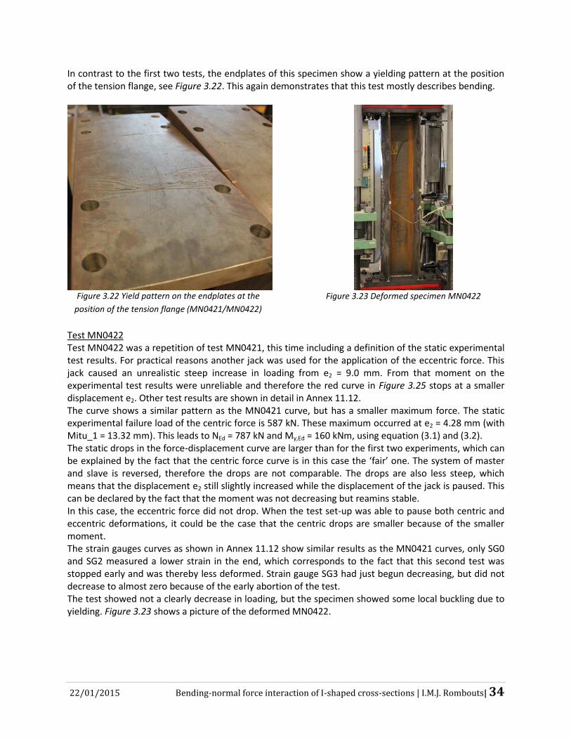
22/01/2015 Bending-normal force interaction of I-shaped cross-sections | I.M.J. Rombouts| 34
In contrast to the first two tests, the endplates of this specimen show a yielding pattern at the position of the tension flange, see Figure 3.22. This again demonstrates that this test mostly describes bending.
Figure 3.22 Yield pattern on the endplates at the
position of the tension flange (MN0421/MN0422)
Figure 3.23 Deformed specimen MN0422
Test MN0422 Test MN0422 was a repetition of test MN0421, this time including a definition of the static experimental test results. For practical reasons another jack was used for the application of the eccentric force. This jack caused an unrealistic steep increase in loading from e2 = 9.0 mm. From that moment on the experimental test results were unreliable and therefore the red curve in Figure 3.25 stops at a smaller displacement e2. Other test results are shown in detail in Annex 11.12. The curve shows a similar pattern as the MN0421 curve, but has a smaller maximum force. The static experimental failure load of the centric force is 587 kN. These maximum occurred at e2 = 4.28 mm (with Mitu_1 = 13.32 mm). This leads to NEd = 787 kN and My,Ed = 160 kNm, using equation (3.1) and (3.2). The static drops in the force-displacement curve are larger than for the first two experiments, which can be explained by the fact that the centric force curve is in this case the ‘fair’ one. The system of master and slave is reversed, therefore the drops are not comparable. The drops are also less steep, which means that the displacement e2 still slightly increased while the displacement of the jack is paused. This can be declared by the fact that the moment was not decreasing but reamins stable. In this case, the eccentric force did not drop. When the test set-up was able to pause both centric and eccentric deformations, it could be the case that the centric drops are smaller because of the smaller moment. The strain gauges curves as shown in Annex 11.12 show similar results as the MN0421 curves, only SG0 and SG2 measured a lower strain in the end, which corresponds to the fact that this second test was stopped early and was thereby less deformed. Strain gauge SG3 had just begun decreasing, but did not decrease to almost zero because of the early abortion of the test. The test showed not a clearly decrease in loading, but the specimen showed some local buckling due to yielding. Figure 3.23 shows a picture of the deformed MN0422.

22/01/2015 Bending-normal force interaction of I-shaped cross-sections | I.M.J. Rombouts| 35
Test MN0431 The last two tests with utilization ratio n = 0.4 are the tests loaded with a constant total normal force. At first, a dynamic constant normal force of roughly 910 kN was applied by the centric jack switched in its force-controlled mode. The value of 910 kN is calculated with the summation of the dynamic forces in the proportional case. Thereafter, the eccentric force was applied with the help of two jacks in the displacement controlled 2.5MN actuator with a test speed of 4 mm/min, which corresponds to 2 mm/min at the 2.5MN actuator. The centric jack follows the eccentric jack by decreasing the centric force to get a stable total NEd. Since the zero reference measurement of the centric force turned out to be incorrect in the end, the centric force is lowered with 8 kN. Therefore this specimen was actually constantly loaded with NEd ≈ 902 kN. The force-deformation curve of this test is shown in yellow in Figure 3.25. In this case the eccentric jack is the master and the centric jack the slave. Since the total normal force had to be stable, the centric force increased while the eccentric force decreased in the plastic branch. The drops in loading (for the eccentric force) are bigger than for the MN041 set, which might be caused by the higher test speed. This could be enhanced by some kind of chain reaction of the forces: the eccentric displacement is paused and therefore dropped the eccentric loading, but the centric loading increased as a reaction on the decreasing eccentric force. This means that for increasing e2 (which increases a little bit) less eccentric force is needed and the curve drops more until the displacement e2 has stabilized. The centric experimental failure load is 704 kN, with an eccentric experimental failure load of 198 kN. These maximums occurred at e2 = 4.44 mm (with Mitu_1 = 12.11 mm). The static eccentric failure load is roughly 0.926 times the dynamic test result (calculated with MN0431), which leads to Fexp,ecc = 183 kN. The static centric failure load is 1.023 times the dynamic test results, as shown in Annex 11.13. Figure 3.24 shows a picture of the deformed MN0431. All three strain gauges measured compression when the centric compression was applied. From the moment that bending was applied, SG0 remained in compression and SG2 and SG3 shifted to tension. Later, SG2 measured compression and SG3 was also moving to zero which again shows that the neutral line is moving to the tension flange during the test.
Figure 3.24 Deformed specimen MN0431 (left), MN0432 (right)
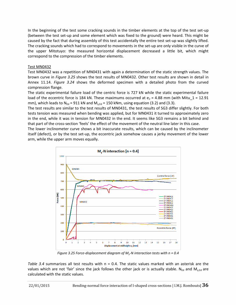
22/01/2015 Bending-normal force interaction of I-shaped cross-sections | I.M.J. Rombouts| 36
In the beginning of the test some cracking sounds in the timber elements at the top of the test set-up (between the test set-up and some element which was fixed to the ground) were heard. This might be caused by the fact that during assembly of this test accidentally the entire test set-up was slightly lifted. The cracking sounds which had to correspond to movements in the set-up are only visible in the curve of the upper Mitotuyo: the measured horizontal displacement decreased a little bit, which might correspond to the compression of the timber elements.
Test MN0432 Test MN0432 was a repetition of MN0431 with again a determination of the static strength values. The brown curve in Figure 3.25 shows the test results of MN0432. Other test results are shown in detail in Annex 11.14. Figure 3.24 shows the deformed specimen with a detailed photo from the curved compression flange. The static experimental failure load of the centric force is 727 kN while the static experimental failure load of the eccentric force is 184 kN. These maximums occurred at e2 = 4.88 mm (with Mitu_1 = 12.91 mm), which leads to NEd = 911 kN and My,Ed = 150 kNm, using equation (3.2) and (3.3). The test results are similar to the test results of MN0431, the test results of SG3 differ slightly. For both tests tension was measured when bending was applied, but for MN0431 it turned to approximately zero in the end, while it was in tension for MN0432 in the end. It seems like SG3 remains a bit behind and that part of the cross-section ‘feels’ the effect of the movement of the neutral line later in this case. The lower inclinometer curve shows a bit inaccurate results, which can be caused by the inclinometer itself (defect), or by the test set-up, the eccentric jack somehow causes a jerky movement of the lower arm, while the upper arm moves equally.
Figure 3.25 Force-displacement diagram of My-N interaction tests with n = 0.4
Table 3.4 summarizes all test results with n = 0.4. The static values marked with an asterisk are the values which are not ‘fair’ since the jack follows the other jack or is actually stable. NEd and My,Ed are calculated with the static values.
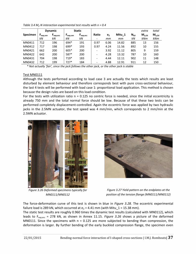
22/01/2015 Bending-normal force interaction of I-shaped cross-sections | I.M.J. Rombouts| 37
Table 3.4 My-N interaction experimental test results with n = 0.4
Dynamic Static extra total Specimen Fexp,cen Fexp,ecc Fexp,cen Fexp,ecc Ratio e2 Mitu_1 NEd My,Ed My,Ed
kN kN kN kN - mm mm kN kNm kNm
MN0411 712 196 694* 191 0.97 6.06 14.82 885 13 156 MN0412 717 198 699* 193 0.97 4.24 11.56 892 10 155 MN0421 662 200 605* 200 - 3.92 11.12 805 9 159 MN0422 642 200 587* 200 - 4.28 13.32 787 10 160 MN0431 704 198 719* 183 - 4.44 12.11 902 11 148 MN0432 712 199 727* 184 - 4.88 12.91 911 12 150
* Not actually ‘fair’, since the jack follows the other jack, or the other jack is stable
Test MN0111 Although the tests performed according to load case 3 are actually the tests which results are least disturbed by element behaviour and therefore corresponds best with pure cross-sectional behaviour, the last 4 tests will be performed with load case 1: proportional load application. This method is chosen because the design rules are based on this load condition. For the tests with utilization ratio n = 0.125 no centric force is needed, since the initial eccentricity is already 750 mm and the total normal force should be low. Because of that these two tests can be performed completely displacement-controlled. Again the eccentric force was applied by two hydraulic jacks in the 2.5MN actuator, the test speed was 4 mm/min, which corresponds to 2 mm/min at the 2.5MN actuator.
Figure 3.26 Deformed specimens typically for
MN0111/MN0112
Figure 3.27 Yield pattern on the endplates at the
position of the tension flange (MN0111/MN0112)
The force-deformation curve of this test is shown in blue in Figure 3.28. The eccentric experimental failure load is 289 kN, which occurred at e2 = 4.41 mm (with Mitu_1 = 15.38 mm). The static test results are roughly 0.960 times the dynamic test results (calculated with MN0112), which leads to Fexp,ecc = 278 kN, as shown in Annex 11.15. Figure 3.26 shows a picture of the deformed MN0111. Since the specimens with n = 0.125 are more subjected to bending than compression, the deformation is larger. By further bending of the early buckled compression flange, the specimen even

22/01/2015 Bending-normal force interaction of I-shaped cross-sections | I.M.J. Rombouts| 38
starts to bend around its weak axis, as shown in the right photo of Figure 3.26. The test was stopped after a clear decrease of the eccentric force and this large deformations. Again three strain gauges measured the strain, but they were positioned as shown in the right picture in Figure 3.18. The neutral line should be theoretically between 1 and 2, which corresponds with the test results: SG0 and SG1 measured compression from the beginning and SG2 measured tension from the beginning. From ε ≈ -0.002 SG2 gave a defect signal, which might be caused by the fact that there was some remaining flake of mill scale under the strain gauge. It is remarkable that Mitu_0 and Mitu_2 (the upper and lower displacement measurement equipment) measured almost equal displacement, which says that it is neatly bended around the strong axis. Test MN0112 Test MN0112 was a repetition test of MN0111 with again three times a drop in loading. The force-deformation curve of this test is shown in orange in Figure 3.28. The eccentric static experimental failure load is also 278 kN, which occurred at e2 = 4.21 mm (with MItu_1 = 15.06 mm), which leads to NEd = 278 kN and My,Ed = 213 kNm. Annex 11.16 shows detailed experimental test results of MN0112. The test results are similar as for test MN0111, but the force-deformation curve differs: from e2 ≈ 10 mm this second specimen can bear higher values of the eccentric force. This difference might be declared by the difference in bending around the weak axis, since the first parts of the curves are similar to each other. Just as for MN0111, Mitu_0 and Mitu_2 measured similar displacements. This is the only configuration for which the strain in tension exceeds the 0.2% proportional limit strain. Also for these two tests the endplates showed yielding lines at the position of the tension flange, as shown in Figure 3.27. This is logical, since the amount of bending is high compared to the amount of normal force. Table 3.5 summarizes all test results with n = 0.125.
Figure 3.28 Force-displacement diagram of My-N interaction tests with n = 0.125

22/01/2015 Bending-normal force interaction of I-shaped cross-sections | I.M.J. Rombouts| 39
Table 3.5 My-N interaction experimental test results with n = 0.125
Dynamic Static extra total Specimen Fexp,cen Fexp,ecc Fexp,cen Fexp,ecc Ratio e2 Mitu_1 NEd My,Ed My,Ed
kN kN kN kN - mm mm kN kNm kNm
MN0111 0 289 0 278 0.96 4.41 15.38 278 4 213 MN0112 0 289 0 278 0.96 4.21 15.06 278 4 213
* Not actually ‘fair’, since the jack follows the other jack, or the other jack is stable
Test MN0611 The last two tests were performed with utilization ratio n = 0.6. The ratio between the eccentric and centric force was 1:9.0. For this case the eccentric force was applied by one hydraulic jack in the 250kN actuator. Moreover, it would surely not exceed 250 kN. The eccentric force was applied with a test speed of 2 mm/min. The centric jack was programmed to follow the eccentric signal and multiply by 9.0, which leads to a force-controlled application of the centric force. The force-deformation curve of this test is shown in purple in Figure 3.30. The centric experimental failure load is 1190 kN, the eccentric experimental failure load is 132 kN, which both occurred at e2 = 3.10 mm (with Mitu_1 = 8.50 mm). The shifted static branch, as shown in Annex 11.17 is calculated with the data of test MN0612. These static test results are roughly 0.953 times the dynamic test results, which leads to Fexp,cen = 1134 kN, and Fexp,ecc = 126 kN. The positions of the strain gauges are similar to the positions of the n = 0.4 tests, since the neutral line is again in the tension flange. In contrast to the n = 0.4 tests, for this test all three strain gauges measured compression in the beginning. Only SG3 measured small tension in the end, which means that the neutral line is nearby. The strain measured in tension is lower than measured for the MN041 tests, which shows that the neutral line is further from SG3, just as in theory. It is surprising that SG3 measured a little bit of compression in the beginning, but it will have to be explained by the fact that SG3 measured in the zone which cannot be characterized well enought, it feels the influence of the neutral line and is not able to reach the 0.2% yield strain. Just like the MN01 tests Mitu_0 and Mitu_2 measured almost equal displacement, which indicates for a neatly bended specimen. Figure 3.29 shows the deformed specimen MN0611.
Figure 3.29 Deformed specimen MN0611 (left) and MN0612 (right)
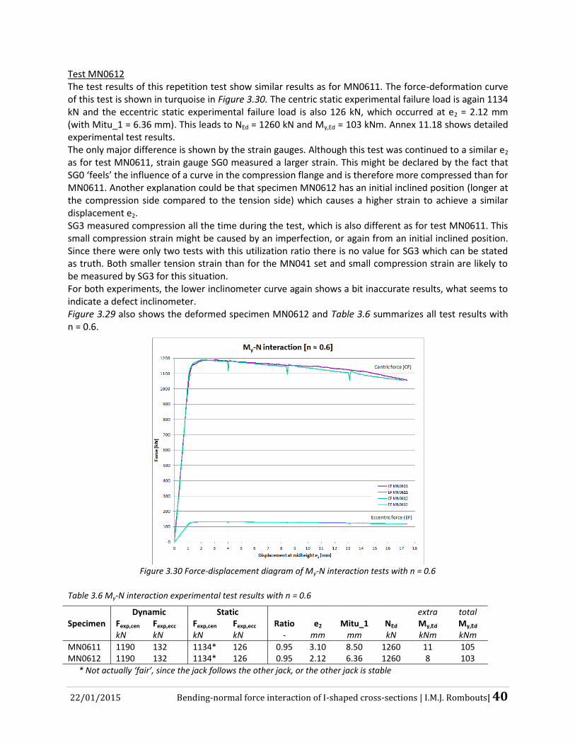
22/01/2015 Bending-normal force interaction of I-shaped cross-sections | I.M.J. Rombouts| 40
Test MN0612 The test results of this repetition test show similar results as for MN0611. The force-deformation curve of this test is shown in turquoise in Figure 3.30. The centric static experimental failure load is again 1134 kN and the eccentric static experimental failure load is also 126 kN, which occurred at e2 = 2.12 mm (with Mitu_1 = 6.36 mm). This leads to NEd = 1260 kN and My,Ed = 103 kNm. Annex 11.18 shows detailed experimental test results. The only major difference is shown by the strain gauges. Although this test was continued to a similar e2 as for test MN0611, strain gauge SG0 measured a larger strain. This might be declared by the fact that SG0 ‘feels’ the influence of a curve in the compression flange and is therefore more compressed than for MN0611. Another explanation could be that specimen MN0612 has an initial inclined position (longer at the compression side compared to the tension side) which causes a higher strain to achieve a similar displacement e2. SG3 measured compression all the time during the test, which is also different as for test MN0611. This small compression strain might be caused by an imperfection, or again from an initial inclined position. Since there were only two tests with this utilization ratio there is no value for SG3 which can be stated as truth. Both smaller tension strain than for the MN041 set and small compression strain are likely to be measured by SG3 for this situation. For both experiments, the lower inclinometer curve again shows a bit inaccurate results, what seems to indicate a defect inclinometer. Figure 3.29 also shows the deformed specimen MN0612 and Table 3.6 summarizes all test results with n = 0.6.
Figure 3.30 Force-displacement diagram of My-N interaction tests with n = 0.6
Table 3.6 My-N interaction experimental test results with n = 0.6
Dynamic Static extra total Specimen Fexp,cen Fexp,ecc Fexp,cen Fexp,ecc Ratio e2 Mitu_1 NEd My,Ed My,Ed
kN kN kN kN - mm mm kN kNm kNm
MN0611 1190 132 1134* 126 0.95 3.10 8.50 1260 11 105 MN0612 1190 132 1134* 126 0.95 2.12 6.36 1260 8 103
* Not actually ‘fair’, since the jack follows the other jack, or the other jack is stable
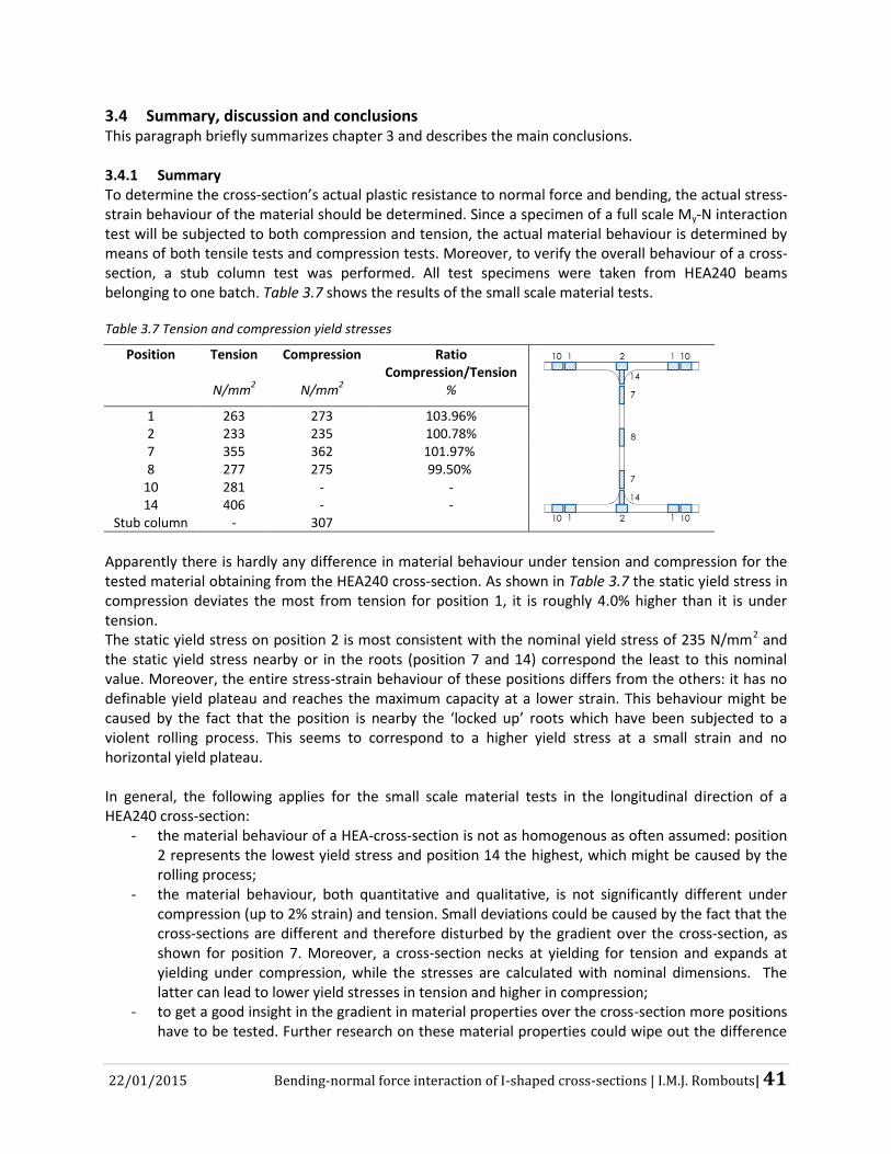
22/01/2015 Bending-normal force interaction of I-shaped cross-sections | I.M.J. Rombouts| 41
3.4 Summary, discussion and conclusions This paragraph briefly summarizes chapter 3 and describes the main conclusions. 3.4.1 Summary To determine the cross-section’s actual plastic resistance to normal force and bending, the actual stress-strain behaviour of the material should be determined. Since a specimen of a full scale My-N interaction test will be subjected to both compression and tension, the actual material behaviour is determined by means of both tensile tests and compression tests. Moreover, to verify the overall behaviour of a cross-section, a stub column test was performed. All test specimens were taken from HEA240 beams belonging to one batch. Table 3.7 shows the results of the small scale material tests.
Table 3.7 Tension and compression yield stresses
Position Tension Compression Ratio Compression/Tension
N/mm
2 N/mm
2 %
1 263 273 103.96% 2 233 235 100.78% 7 355 362 101.97% 8 277 275 99.50%
10 281 - - 14 406 - -
Stub column - 307
Apparently there is hardly any difference in material behaviour under tension and compression for the tested material obtaining from the HEA240 cross-section. As shown in Table 3.7 the static yield stress in compression deviates the most from tension for position 1, it is roughly 4.0% higher than it is under tension. The static yield stress on position 2 is most consistent with the nominal yield stress of 235 N/mm2 and the static yield stress nearby or in the roots (position 7 and 14) correspond the least to this nominal value. Moreover, the entire stress-strain behaviour of these positions differs from the others: it has no definable yield plateau and reaches the maximum capacity at a lower strain. This behaviour might be caused by the fact that the position is nearby the ‘locked up’ roots which have been subjected to a violent rolling process. This seems to correspond to a higher yield stress at a small strain and no horizontal yield plateau. In general, the following applies for the small scale material tests in the longitudinal direction of a HEA240 cross-section:
- the material behaviour of a HEA-cross-section is not as homogenous as often assumed: position 2 represents the lowest yield stress and position 14 the highest, which might be caused by the rolling process;
- the material behaviour, both quantitative and qualitative, is not significantly different under compression (up to 2% strain) and tension. Small deviations could be caused by the fact that the cross-sections are different and therefore disturbed by the gradient over the cross-section, as shown for position 7. Moreover, a cross-section necks at yielding for tension and expands at yielding under compression, while the stresses are calculated with nominal dimensions. The latter can lead to lower yield stresses in tension and higher in compression;
- to get a good insight in the gradient in material properties over the cross-section more positions have to be tested. Further research on these material properties could wipe out the difference

22/01/2015 Bending-normal force interaction of I-shaped cross-sections | I.M.J. Rombouts| 42
in calculated global static yield strength over the cross-section and the global static yield strength determined with the stub column test.
To test the actual behaviour of a doubly symmetrical I-shaped cross-section subjected to combined strong axis bending and normal force, a specific test-set up was designed (see Figure 3.31 for the principle). Ten specimens (5 different tests with each 2 specimens) were subjected to combined bending and normal force without interference of other mechanisms like buckling and lateral-torsional buckling. The specimens were tested for three utilization ratios: n = 0.125, n = 0.4 and n = 0.6.
Figure 3.31 Principle of the test set-up
The different options in load application of the six specimens loaded with utilization ratio n = 0.4 (3x2) formed another experiment. Three different load cases were determined:
1. Proportionally: NEd,ecc and NEd,cen both increase in a predetermined ratio. 2. Constant moment (MEd): the moment which is adjusted from the proportional tests will be
applied by NEd,ecc, thereafter NEd,cen will increase. 3. Constant normal force (NEd): the normal force which is adjusted from the proportional test will
be applied as NEd,cen. While NEd,ecc increases, NEd,cen decreases in a way that NEd remains constant. Although load case 3 should actually be the load case which results should be less disturbed by an extra moment due eccentricity caused by bending, the last 4 tests were performed with load case 1: proportional load application. This is because the design rules are also based on this load condition. Overall, the force-deformation curves show a clear elastic branch followed by a decreasing plastic branch, which might be caused by the small extra moment due to increasing eccentricity. The utilization ratios are therefore not stable during the tests, since the bending moment increases while the normal force decreases. The maximum force which is reached just after the start of the plastic branch is stated as the experimental ‘failure’ load which is used to determine the experimental failure NEd and My,Ed. Table 3.8 summarizes all My-N interaction experimental test results. The name of the specimens can be declared as follows: the first two numbers define the utilization ratio n, the third number displays the load case as mentioned before and the last number shows the specimen number. The static values are not always ‘fair’, since the application of loading is in almost all cases a system of one jack following the other jack. Only one jack shows an actual drop in loading, the static value for the other loading follows the actual drop from the master jack. Values which for that reason are not fair are marked with an asterisk. Due to the proportional load application, the utilization ratios are not exactly as predefined (n = 0.125, n = 0.4 and n = 0.6), since both normal force and moment were increasing.
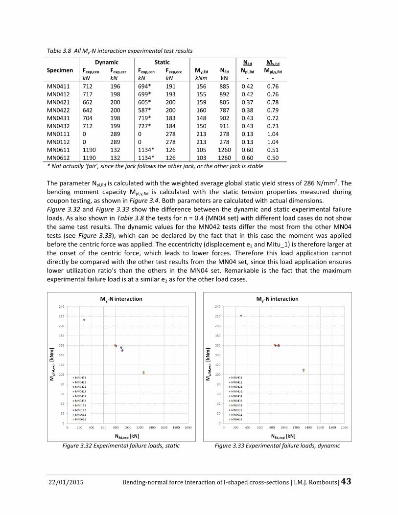
22/01/2015 Bending-normal force interaction of I-shaped cross-sections | I.M.J. Rombouts| 43
Table 3.8 All My-N interaction experimental test results
Dynamic Static NEd My,Ed
Specimen Fexp,cen Fexp,ecc Fexp,cen Fexp,ecc My,Ed NEd Npl,Rd Mpl,y,Rd
kN kN kN kN kNm kN - -
MN0411 712 196 694* 191 156 885 0.42 0.76 MN0412 717 198 699* 193 155 892 0.42 0.76 MN0421 662 200 605* 200 159 805 0.37 0.78 MN0422 642 200 587* 200 160 787 0.38 0.79 MN0431 704 198 719* 183 148 902 0.43 0.72 MN0432 712 199 727* 184 150 911 0.43 0.73 MN0111 0 289 0 278 213 278 0.13 1.04 MN0112 0 289 0 278 213 278 0.13 1.04 MN0611 1190 132 1134* 126 105 1260 0.60 0.51 MN0612 1190 132 1134* 126 103 1260 0.60 0.50
* Not actually ‘fair’, since the jack follows the other jack, or the other jack is stable
The parameter Npl,Rd is calculated with the weighted average global static yield stress of 286 N/mm2. The bending moment capacity Mpl,y,Rd is calculated with the static tension properties measured during coupon testing, as shown in Figure 3.4. Both parameters are calculated with actual dimensions. Figure 3.32 and Figure 3.33 show the difference between the dynamic and static experimental failure loads. As also shown in Table 3.8 the tests for n = 0.4 (MN04 set) with different load cases do not show the same test results. The dynamic values for the MN042 tests differ the most from the other MN04 tests (see Figure 3.33), which can be declared by the fact that in this case the moment was applied before the centric force was applied. The eccentricity (displacement e2 and Mitu_1) is therefore larger at the onset of the centric force, which leads to lower forces. Therefore this load application cannot directly be compared with the other test results from the MN04 set, since this load application ensures lower utilization ratio’s than the others in the MN04 set. Remarkable is the fact that the maximum experimental failure load is at a similar e2 as for the other load cases.
Figure 3.32 Experimental failure loads, static
Figure 3.33 Experimental failure loads, dynamic
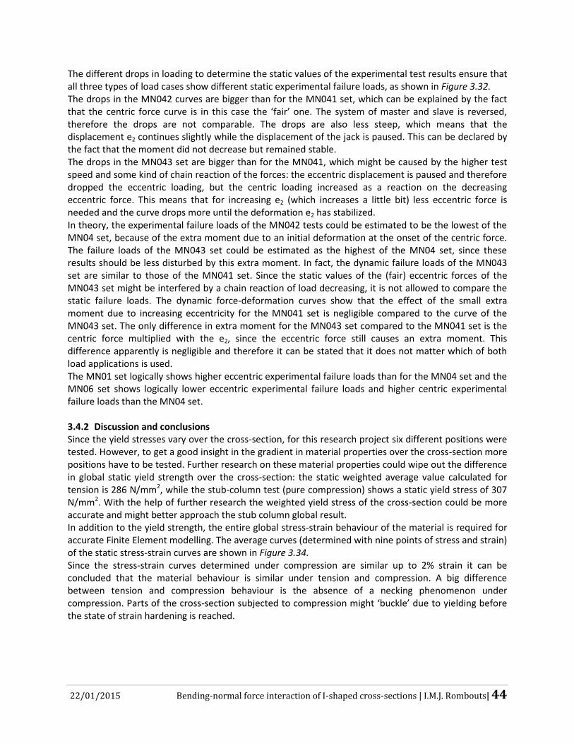
22/01/2015 Bending-normal force interaction of I-shaped cross-sections | I.M.J. Rombouts| 44
The different drops in loading to determine the static values of the experimental test results ensure that all three types of load cases show different static experimental failure loads, as shown in Figure 3.32. The drops in the MN042 curves are bigger than for the MN041 set, which can be explained by the fact that the centric force curve is in this case the ‘fair’ one. The system of master and slave is reversed, therefore the drops are not comparable. The drops are also less steep, which means that the displacement e2 continues slightly while the displacement of the jack is paused. This can be declared by the fact that the moment did not decrease but remained stable. The drops in the MN043 set are bigger than for the MN041, which might be caused by the higher test speed and some kind of chain reaction of the forces: the eccentric displacement is paused and therefore dropped the eccentric loading, but the centric loading increased as a reaction on the decreasing eccentric force. This means that for increasing e2 (which increases a little bit) less eccentric force is needed and the curve drops more until the deformation e2 has stabilized. In theory, the experimental failure loads of the MN042 tests could be estimated to be the lowest of the MN04 set, because of the extra moment due to an initial deformation at the onset of the centric force. The failure loads of the MN043 set could be estimated as the highest of the MN04 set, since these results should be less disturbed by this extra moment. In fact, the dynamic failure loads of the MN043 set are similar to those of the MN041 set. Since the static values of the (fair) eccentric forces of the MN043 set might be interfered by a chain reaction of load decreasing, it is not allowed to compare the static failure loads. The dynamic force-deformation curves show that the effect of the small extra moment due to increasing eccentricity for the MN041 set is negligible compared to the curve of the MN043 set. The only difference in extra moment for the MN043 set compared to the MN041 set is the centric force multiplied with the e2, since the eccentric force still causes an extra moment. This difference apparently is negligible and therefore it can be stated that it does not matter which of both load applications is used. The MN01 set logically shows higher eccentric experimental failure loads than for the MN04 set and the MN06 set shows logically lower eccentric experimental failure loads and higher centric experimental failure loads than the MN04 set. 3.4.2 Discussion and conclusions Since the yield stresses vary over the cross-section, for this research project six different positions were tested. However, to get a good insight in the gradient in material properties over the cross-section more positions have to be tested. Further research on these material properties could wipe out the difference in global static yield strength over the cross-section: the static weighted average value calculated for tension is 286 N/mm2, while the stub-column test (pure compression) shows a static yield stress of 307 N/mm2. With the help of further research the weighted yield stress of the cross-section could be more accurate and might better approach the stub column global result. In addition to the yield strength, the entire global stress-strain behaviour of the material is required for accurate Finite Element modelling. The average curves (determined with nine points of stress and strain) of the static stress-strain curves are shown in Figure 3.34. Since the stress-strain curves determined under compression are similar up to 2% strain it can be concluded that the material behaviour is similar under tension and compression. A big difference between tension and compression behaviour is the absence of a necking phenomenon under compression. Parts of the cross-section subjected to compression might ‘buckle’ due to yielding before the state of strain hardening is reached.
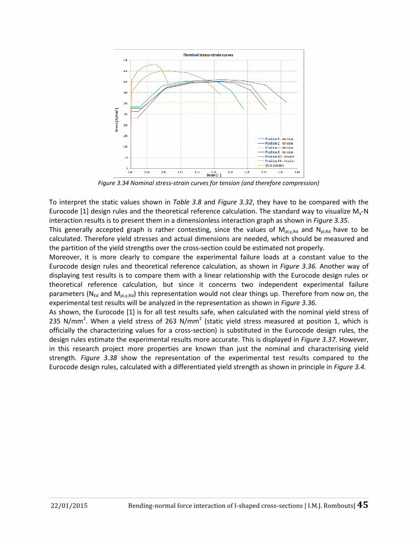
22/01/2015 Bending-normal force interaction of I-shaped cross-sections | I.M.J. Rombouts| 45
Figure 3.34 Nominal stress-strain curves for tension (and therefore compression)
To interpret the static values shown in Table 3.8 and Figure 3.32, they have to be compared with the Eurocode [1] design rules and the theoretical reference calculation. The standard way to visualize My-N interaction results is to present them in a dimensionless interaction graph as shown in Figure 3.35. This generally accepted graph is rather contesting, since the values of Mpl,y,Rd and Npl,Rd have to be calculated. Therefore yield stresses and actual dimensions are needed, which should be measured and the partition of the yield strengths over the cross-section could be estimated not properly. Moreover, it is more clearly to compare the experimental failure loads at a constant value to the Eurocode design rules and theoretical reference calculation, as shown in Figure 3.36. Another way of displaying test results is to compare them with a linear relationship with the Eurocode design rules or theoretical reference calculation, but since it concerns two independent experimental failure parameters (NEd and Mpl,y,Rd) this representation would not clear things up. Therefore from now on, the experimental test results will be analyzed in the representation as shown in Figure 3.36. As shown, the Eurocode [1] is for all test results safe, when calculated with the nominal yield stress of 235 N/mm2. When a yield stress of 263 N/mm2 (static yield stress measured at position 1, which is officially the characterizing values for a cross-section) is substituted in the Eurocode design rules, the design rules estimate the experimental results more accurate. This is displayed in Figure 3.37. However, in this research project more properties are known than just the nominal and characterising yield strength. Figure 3.38 show the representation of the experimental test results compared to the Eurocode design rules, calculated with a differentiated yield strength as shown in principle in Figure 3.4.

22/01/2015 Bending-normal force interaction of I-shaped cross-sections | I.M.J. Rombouts| 46
Figure 3.35 Dimensionless My-N interaction curve of the
test results (fy = 235 N/mm2)
Figure 3.36 My-N interaction curve of the test results
(fy = 235 N/mm2)
As shown, the Eurocode [1] expects higher resistance to normal force and bending moment, which leads to a more accurate prediction of the experimental failure loads. This material model is more in line with the actual material behaviour than the material models before.
Figure 3.37 My-N interaction curve of the test results
(fy = 263 N/mm2)
Figure 3.38 My-N interaction curve of the test results
(fy = differentiated) One step further is to use the static yield strength determinated during the stub column test, which is 307 N/mm2. The Eurocode overestimates the experimental tests results, as shown in Figure 3.39. Since the overall material behaviour of the specimens subjected to combined bending and normal force should be somewhere in between these two material models, the design rules could be just safe.
fy = 235 N/mm2
fy = 235 N/mm2
fy = 263 N/mm2
fy = differentiated
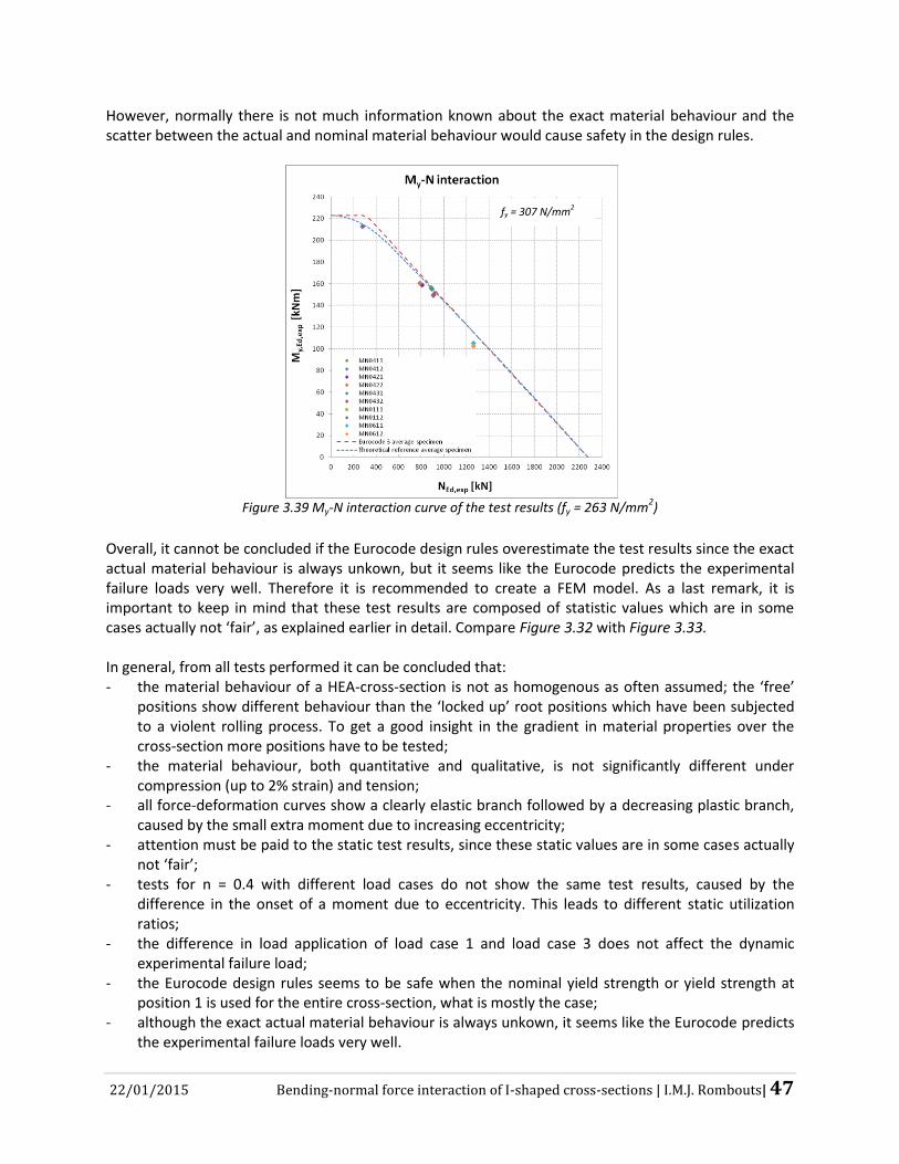
22/01/2015 Bending-normal force interaction of I-shaped cross-sections | I.M.J. Rombouts| 47
However, normally there is not much information known about the exact material behaviour and the scatter between the actual and nominal material behaviour would cause safety in the design rules.
Figure 3.39 My-N interaction curve of the test results (fy = 263 N/mm
2)
Overall, it cannot be concluded if the Eurocode design rules overestimate the test results since the exact actual material behaviour is always unkown, but it seems like the Eurocode predicts the experimental failure loads very well. Therefore it is recommended to create a FEM model. As a last remark, it is important to keep in mind that these test results are composed of statistic values which are in some cases actually not ‘fair’, as explained earlier in detail. Compare Figure 3.32 with Figure 3.33. In general, from all tests performed it can be concluded that: - the material behaviour of a HEA-cross-section is not as homogenous as often assumed; the ‘free’
positions show different behaviour than the ‘locked up’ root positions which have been subjected to a violent rolling process. To get a good insight in the gradient in material properties over the cross-section more positions have to be tested;
- the material behaviour, both quantitative and qualitative, is not significantly different under compression (up to 2% strain) and tension;
- all force-deformation curves show a clearly elastic branch followed by a decreasing plastic branch, caused by the small extra moment due to increasing eccentricity;
- attention must be paid to the static test results, since these static values are in some cases actually not ‘fair’;
- tests for n = 0.4 with different load cases do not show the same test results, caused by the difference in the onset of a moment due to eccentricity. This leads to different static utilization ratios;
- the difference in load application of load case 1 and load case 3 does not affect the dynamic experimental failure load;
- the Eurocode design rules seems to be safe when the nominal yield strength or yield strength at position 1 is used for the entire cross-section, what is mostly the case;
- although the exact actual material behaviour is always unkown, it seems like the Eurocode predicts the experimental failure loads very well.
fy = 307 N/mm2
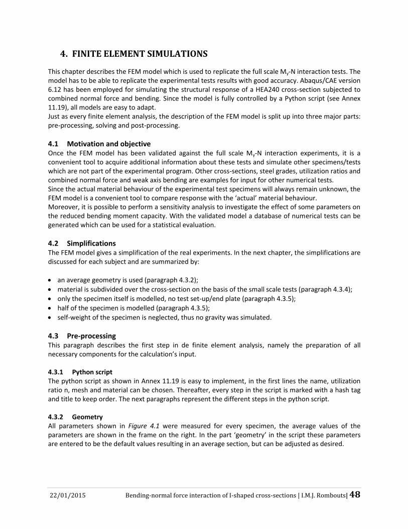
22/01/2015 Bending-normal force interaction of I-shaped cross-sections | I.M.J. Rombouts| 48
4. FINITE ELEMENT SIMULATIONS
This chapter describes the FEM model which is used to replicate the full scale My-N interaction tests. The model has to be able to replicate the experimental tests results with good accuracy. Abaqus/CAE version 6.12 has been employed for simulating the structural response of a HEA240 cross-section subjected to combined normal force and bending. Since the model is fully controlled by a Python script (see Annex 11.19), all models are easy to adapt. Just as every finite element analysis, the description of the FEM model is split up into three major parts: pre-processing, solving and post-processing.
4.1 Motivation and objective Once the FEM model has been validated against the full scale My-N interaction experiments, it is a convenient tool to acquire additional information about these tests and simulate other specimens/tests which are not part of the experimental program. Other cross-sections, steel grades, utilization ratios and combined normal force and weak axis bending are examples for input for other numerical tests. Since the actual material behaviour of the experimental test specimens will always remain unknown, the FEM model is a convenient tool to compare response with the ‘actual’ material behaviour. Moreover, it is possible to perform a sensitivity analysis to investigate the effect of some parameters on the reduced bending moment capacity. With the validated model a database of numerical tests can be generated which can be used for a statistical evaluation.
4.2 Simplifications The FEM model gives a simplification of the real experiments. In the next chapter, the simplifications are discussed for each subject and are summarized by:
an average geometry is used (paragraph 4.3.2);
material is subdivided over the cross-section on the basis of the small scale tests (paragraph 4.3.4);
only the specimen itself is modelled, no test set-up/end plate (paragraph 4.3.5);
half of the specimen is modelled (paragraph 4.3.5);
self-weight of the specimen is neglected, thus no gravity was simulated.
4.3 Pre-processing This paragraph describes the first step in de finite element analysis, namely the preparation of all necessary components for the calculation’s input. 4.3.1 Python script The python script as shown in Annex 11.19 is easy to implement, in the first lines the name, utilization ratio n, mesh and material can be chosen. Thereafter, every step in the script is marked with a hash tag and title to keep order. The next paragraphs represent the different steps in the python script. 4.3.2 Geometry All parameters shown in Figure 4.1 were measured for every specimen, the average values of the parameters are shown in the frame on the right. In the part ‘geometry’ in the script these parameters are entered to be the default values resulting in an average section, but can be adjusted as desired.

22/01/2015 Bending-normal force interaction of I-shaped cross-sections | I.M.J. Rombouts| 49
Figure 4.1 Parameters of the geometry
4.3.3 Elements To optimise the FEM model the exact geometry (including the fillets) has to be entered, therefore the 3D solid element is chosen. After the geometry step was completed by sketching the 2D profile, the sketch has to be extruded to a 3D solid body with a length of 600 mm (half of the specimen, see paragraph 4.3.5). 4.3.4 Material The measured engineering stresses and strains do not meet the requirements of a geometric non-linear analysis, because the strains and stresses are calculated with its nominal cross-section and nominal gauge length. Therefore the engineering stresses and strains are conversed to true stresses and strains according to equation (4.1) to (4.4). These formulas take into account the current dimensions. The stress-strain curves measured for tension define the material response for both tension and compression in the FEM model.
σtrue = σnom ∙ (1 + εnom) (4.1)
εtrue = ln ∙ (1 + εnom) (4.2)
E = σtrue εtrue
(4.3)
εpl = εtrue -
σtrue E (4.4)
In which: σtrue True stress N/mm
2
σnom Engineering stress N/mm2
εtrue True strain - εnom Engineering strain -
εpl True plastic strain -
E Modulus of elasticity N/mm2
Default values (average) h = 234.5 mm tf = 11.1 mm tw = 7.8 mm r = 21 mm b = 116.65 mm
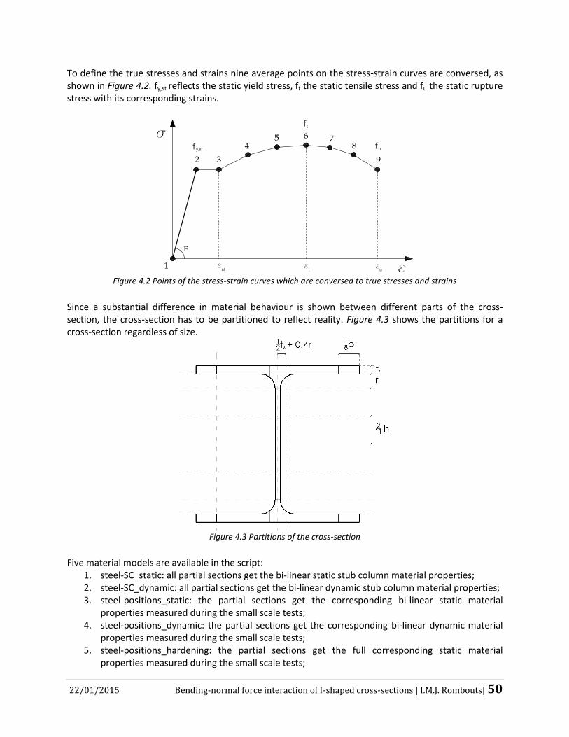
22/01/2015 Bending-normal force interaction of I-shaped cross-sections | I.M.J. Rombouts| 50
To define the true stresses and strains nine average points on the stress-strain curves are conversed, as shown in Figure 4.2. fy,st reflects the static yield stress, ft the static tensile stress and fu the static rupture stress with its corresponding strains.
Figure 4.2 Points of the stress-strain curves which are conversed to true stresses and strains
Since a substantial difference in material behaviour is shown between different parts of the cross-section, the cross-section has to be partitioned to reflect reality. Figure 4.3 shows the partitions for a cross-section regardless of size.
Figure 4.3 Partitions of the cross-section
Five material models are available in the script:
1. steel-SC_static: all partial sections get the bi-linear static stub column material properties; 2. steel-SC_dynamic: all partial sections get the bi-linear dynamic stub column material properties; 3. steel-positions_static: the partial sections get the corresponding bi-linear static material
properties measured during the small scale tests; 4. steel-positions_dynamic: the partial sections get the corresponding bi-linear dynamic material
properties measured during the small scale tests; 5. steel-positions_hardening: the partial sections get the full corresponding static material
properties measured during the small scale tests;

22/01/2015 Bending-normal force interaction of I-shaped cross-sections | I.M.J. Rombouts| 51
The different material models of static and dynamic material properties are included since the static experimental test results are not always ‘fair’. Therefore it is necessary to assess the dynamic and static test results with both a static and dynamic FEM model. Since the primary stresses and secondary stresses due to instability caused by yielding have the same direction and the measured strains are small (max roughly 2.5%), the bi-linear behaviour corresponds more to the experimental test results than the material behaviour with strain hardening included [17]. The strain hardening material model shows an increasing force-deformation curve, instead of constantly decreasing from a certain point. 4.3.5 Boundary conditions Several boundary conditions are applied to the FEM model, as shown in Figure 4.4. Only half a specimen is modelled, taking advantage of symmetry. At mid-height of the specimen (thus at the bottom of the specimen in the model) a symmetric boundary condition is applied, which means that U3 = UR1 = UR2 = 0 for the entire cross-section. U represents displacements, while UR represents rotations. Besides the reduced number of elements and calculation time due to the symmetric boundary condition, it is easier to apply a constant bending moment over the specimen without restraining it at the supports. In addition, a displacement controlled boundary condition is placed at mid-height of the specimen, which restrains U1 to be zero.
Figure 4.4 Boundary conditions in the FEM model
Figure 4.5 Rotations points of the test set-up
The top of the specimen is tied with a stiff element to a point at 346 mm higher, which represents the rotation point in the experimental test set up, as shown in Figure 4.5 by the red dots. At this point U2 and UR3 are constrained to be zero. Since the stiff element is also HEA-shaped, the cross-section remains plane at the top without any boundary condition or constraint.

22/01/2015 Bending-normal force interaction of I-shaped cross-sections | I.M.J. Rombouts| 52
4.3.6 Loading Since both loadings increase proportionally for load case 1, both eccentric as centric loads are defined in one step. The centric load is dependent on the eccentric load in a predefined way. For example for n = 0.4 it holds that Ncen = 3.6 ∙ Necc. The moment is applied by means of two concentrated forces (a tension-compression couple) at the top and bottom of the flanges. The centric force (which represents Necc + Ncen) is also applied as a concentrated force, as shown in Figure 4.6.
Figure 4.6 Loading in the FEM model
4.3.7 Mesh Mesh refinements have been performed on the test at an utilization ratio of n = 0.4 with the dynamic stub column material properties. Table 4.1 presents all results of the parameters which are of interest in the mesh density study and the differences with respect to the experimental test results. Figure 4.7 shows the representation of the meshes.
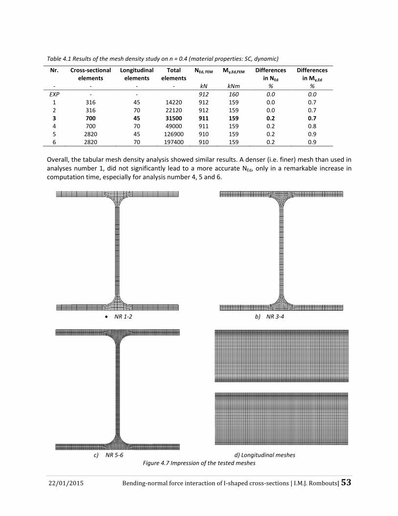
22/01/2015 Bending-normal force interaction of I-shaped cross-sections | I.M.J. Rombouts| 53
Table 4.1 Results of the mesh density study on n = 0.4 (material properties: SC, dynamic)
Nr. Cross-sectional elements
Longitudinal elements
Total elements
NEd, FEM My,Ed,FEM Differences in NEd
Differences in My,Ed
- - - - kN kNm % %
EXP - - 912 160 0.0 0.0 1 316 45 14220 912 159 0.0 0.7 2 316 70 22120 912 159 0.0 0.7 3 700 45 31500 911 159 0.2 0.7 4 700 70 49000 911 159 0.2 0.8 5 2820 45 126900 910 159 0.2 0.9 6 2820 70 197400 910 159 0.2 0.9
Overall, the tabular mesh density analysis showed similar results. A denser (i.e. finer) mesh than used in analyses number 1, did not significantly lead to a more accurate NEd, only in a remarkable increase in computation time, especially for analysis number 4, 5 and 6.
NR 1-2 b) NR 3-4
c) NR 5-6 d) Longitudinal meshes
Figure 4.7 Impression of the tested meshes
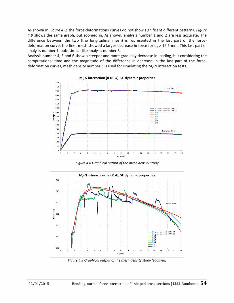
22/01/2015 Bending-normal force interaction of I-shaped cross-sections | I.M.J. Rombouts| 54
As shown in Figure 4.8, the force-deformations curves do not show significant different patterns. Figure 4.9 shows the same graph, but zoomed in. As shown, analysis number 1 and 2 are less accurate. The difference between the two (the longitudinal mesh) is represented in the last part of the force-deformation curve: the finer mesh showed a larger decrease in force for e2 > 16.5 mm. This last part of analysis number 1 looks similar like analysis number 3. Analysis number 4, 5 and 6 show a steeper and more gradually decrease in loading, but considering the computational time and the magnitude of the difference in decrease in the last part of the force-deformation curves, mesh density number 3 is used for simulating the My-N interaction tests.
Figure 4.8 Graphical output of the mesh density study
Figure 4.9 Graphical output of the mesh density study (zoomed)

22/01/2015 Bending-normal force interaction of I-shaped cross-sections | I.M.J. Rombouts| 55
The stiff element has a courser mesh, since the material response does not matter; it only has to be stiff. The elements are all 8-node linear bricks, since the transformation to 20-node quadratic bricks leads besides an increase in computational time, to similar results. The number of elements can easily be adopted in the Python script in the section ‘seed edges’ or at the top of the script, by changing ‘large’ (analysis number 3) into ‘small’ (analysis number 5), which directly leads to a two-fold smaller cross-section mesh density than the default ‘large’ mesh density.
4.4 Solving To apply the loading, a new step subsequent to the initial step is created. Since a ‘Static, General’ step is unable to calculate a negative stiffness of the load-displacement response, the Riks method is used (‘Static, Riks step’). The Riks method solves simultaneously for loads and displacements. To measure the progress of the solution, Abaqus uses the ‘arc length’ along the static equilibrium path in the load-displacement curve [16]. To get a global idea about the load-displacement curve the arc length increment can be determined to be automatic, which allows Abaqus to choose the size of the arc length increments based on computation efficiency. For a more detailed curve, in particular for the elasto-plastic branch, the arc length increment should be fixed at 0.05. Of course the option for the inclusion of geometric nonlinear effects is toggled on in the loading step, leading to a Geometrical Material Non-linear Analysis (GMNA). When an experiment on the load application is modelled, a new (static, general) step has to be created to apply one loading before the other one.
4.5 Post-processing In the post-processor nodal output variables (i.e. load, displacement and strain) were saved. These data were analyzed and edited in Microsoft Excel to validate the FEM model.
4.6 Validation of the FEM model In this paragraph the FEM model will be validated against the experimental load-displacement curves discussed in chapter 3. Since it is not possible for all experiments possible to determine the static experimental failure load, both numerical dynamic and static load-displacement curves are shown in the graphs. The static curves are somewhat schematized. Figure 4.10 shows the general behaviour of half a specimen subjected to combined bending and normal force. The first picture is the start of the test, there is no yielding (red). The second picture shows yielding of the compression flange and web. In the last stage also a part of the tension flange (depending on the position of the neutral line and therefore utilization ratio n) yields. Moreover, the compression flange is curved due to yielding.

22/01/2015 Bending-normal force interaction of I-shaped cross-sections | I.M.J. Rombouts| 56
Figure 4.10 Stages during the numerical tests (red = yielding), 3D view, 2D view and graphical view
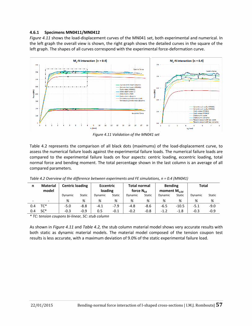
22/01/2015 Bending-normal force interaction of I-shaped cross-sections | I.M.J. Rombouts| 57
4.6.1 Specimens MN0411/MN0412 Figure 4.11 shows the load-displacement curves of the MN041 set, both experimental and numerical. In the left graph the overall view is shown, the right graph shows the detailed curves in the square of the left graph. The shapes of all curves correspond with the experimental force-deformation curve.
Figure 4.11 Validation of the MN041 set
Table 4.2 represents the comparison of all black dots (maximums) of the load-displacement curve, to assess the numerical failure loads against the experimental failure loads. The numerical failure loads are compared to the experimental failure loads on four aspects: centric loading, eccentric loading, total normal force and bending moment. The total percentage shown in the last column is an average of all compared parameters.
Table 4.2 Overview of the difference between experiments and FE simulations, n = 0.4 (MN041)
n Material model
Centric loading Eccentric loading
Total normal force NEd
Bending moment My,Ed
Total
Dynamic Static Dynamic Static Dynamic Static Dynamic Static Dynamic Static
- - % % % % % % % % % %
0.4 TC* -5.0 -8.8 -4.1 -7.9 -4.8 -8.6 -6.5 -10.5 -5.1 -9.0 0.4 SC* -0.3 -0.9 0.5 -0.1 -0.2 -0.8 -1.2 -1.8 -0.3 -0.9
* TC: tension coupons bi-linear, SC: stub column
As shown in Figure 4.11 and Table 4.2, the stub column material model shows very accurate results with both static as dynamic material models. The material model composed of the tension coupon test results is less accurate, with a maximum deviation of 9.0% of the static experimental failure load.

22/01/2015 Bending-normal force interaction of I-shaped cross-sections | I.M.J. Rombouts| 58
4.6.2 Specimens MN0421/MN0422 For the validation of the other load application tests, a new ‘Static, General’ step is created to apply a constant bending moment. The subsequent ‘Static, Riks’ step includes the centric normal force. The force-deformation curves of these tests are shown in Figure 4.12. Since the moment was applied force-controlled, this is nor a static neither a dynamic loading, it is equal for all cases: Necc = 200 kN. Therefore, the difference between numerical and experimental test results for the eccentric force and bending moment in Table 4.3 are zero respectively very small.
Figure 4.12 Validation of the MN042 set
This case show big differences between the load displacement curves of the numerical material models, which might be caused by the constant bending moment of 150 kNm (and an centric force of 200 kN), for all cases. Since every cross-section with a different material model is subjected to the same bending moment there is a difference in ‘place’ left over for the centric normal force. This is why the neutral line for the case with dynamic stub column material properties (highest average yield stress) is positioned more in the flanges while the neutral line in the material model based on static tension coupon results is more in the roots. Overall, applying a constant moment to cross-sections with different material models leads to different utilization ratios n. Small differences is material models can lead to big differences in the force-deformation curve of this kind of test, while the stub column material model shows good accuracy with the experimental results (max 2.6% deviation), as shown in Table 4.3.
Table 4.3 Overview of the difference between experiments and FE simulations, n = 0.4 (MN042)
n Material model
Centric loading Eccentric loading
Total normal force NEd
Bending moment My,Ed
Total
Dynamic Static Dynamic Static Dynamic Static Dynamic Static Dynamic Static
- - % % % % % % % % % %
0.4 TC* -8.6 -25.8 0.0 0.0 -6.5 -18.2 0.1 -0.5 -3.7 -11.1 0.4 SC* 6.5 5.3 0.0 0.0 5.0 4.0 -0.9 -0.9 2.6 2.1
* TC: tension coupons bi-linear, SC: stub column

22/01/2015 Bending-normal force interaction of I-shaped cross-sections | I.M.J. Rombouts| 59
4.6.3 Specimens MN0431/MN0432 For this load application, the total normal force is applied in the initial ‘Static, General’ step. As a constant value of NEd = 907 kN (average of the experimental failure loads). Therefore, the difference between numerical and experimental test results for total normal force in Table 4.4 is zero for both static as dynamic values. The subsequent ‘Static, Riks’ step includes the application of the bending moment. The force-deformation curves of these tests are shown in Figure 4.13.
Figure 4.13 Validation of the MN043 set
For this case, a fixed NEd did not lead to very big differences in the force-deformation graph, since this NEd is divided between Necc (My,Ed) and Ncen and no one should be stable. The stub column material models show good accuracy with the experimental test results. Both models show average results which are lower than the experimental test results. The model based on the bi-linear tension coupon material behaviour shows once again better results regarding the dynamic simulation than using the static simulation.
Table 4.4 Overview of the difference between experiments and FE simulations, n = 0.4 (MN043)
n Material model
Centric loading Eccentric loading
Total normal force NEd
Bending moment My,Ed
Total
Dynamic Static Dynamic Static Dynamic Static Dynamic Static Dynamic Static
- - % % % % % % % % % %
0.4 TC* 2.0 2.5 -8.1 -12.0 0.0 0.0 -9.8 -13.7 -3.9 -5.9 0.4 SC* 0.0 -0.7 0.0 1.6 0.0 0.0 -0.6 0.9 -0.2 -0.4
* TC: tension coupons bi-linear, SC: stub column

22/01/2015 Bending-normal force interaction of I-shaped cross-sections | I.M.J. Rombouts| 60
4.6.4 Specimens MN0111/MN0112 Figure 4.14 shows the load-displacement curves of the MN01 set, both experimental as numerical. Again in the left graph the overall view is shown, the right graph shows the detailed curves in the square of the left graph. The shapes of all curves correspond with the experimental force-deformation curve, although the decrease in loading is smaller. This might be explained by the fact that the specimens started to bend around the weak axis due to yielding at a certain point and a high bending moment. In the FEM model, this will be not the case since yielding occurs at the same time at both sides of the specimen because of the perfect symmetric cross-section. Therefore there is no part less weak than its opposite and the specimen will not start to bend around the weak axis.
Figure 4.14 Validation of the MN011 set
Table 4.2 shows the overview of the difference between experimental test results and numerical test results. The stub column material model shows once again good accuracy with the experimental test results, while the material model based on bi-linear tension coupon test results show less accurate results (on the safe side).
Table 4.5 Overview of the difference between experiments and FE simulations, n = 0.125 (MN01)
n Material model
Centric loading Eccentric loading
Total normal force NEd
Bending moment My,Ed
Total
Dynamic Static Dynamic Static Dynamic Static Dynamic Static Dynamic Static
- - % % % % % % % % % %
0.125 TC* - - -5.3 -7.6 -5.3 -7.6 -5.3 -7.5 -5.3 -7.6 0.125 SC* - - 0.3 1.0 0.3 1.0 0.2 0.9 0.3 1.0
* TC: tension coupons bi-linear, SC: stub column
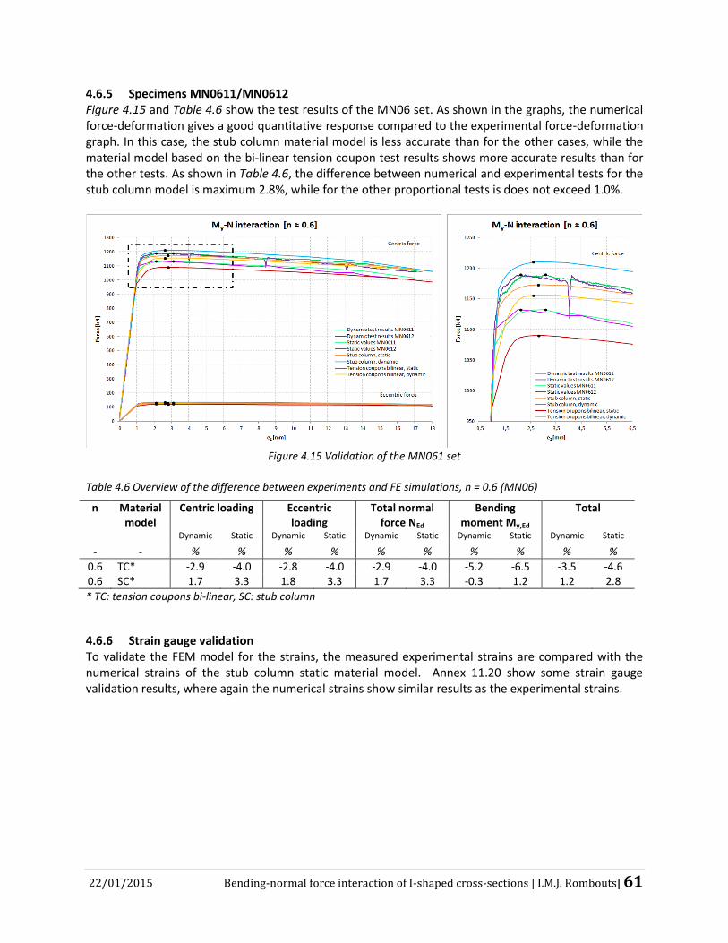
22/01/2015 Bending-normal force interaction of I-shaped cross-sections | I.M.J. Rombouts| 61
4.6.5 Specimens MN0611/MN0612 Figure 4.15 and Table 4.6 show the test results of the MN06 set. As shown in the graphs, the numerical force-deformation gives a good quantitative response compared to the experimental force-deformation graph. In this case, the stub column material model is less accurate than for the other cases, while the material model based on the bi-linear tension coupon test results shows more accurate results than for the other tests. As shown in Table 4.6, the difference between numerical and experimental tests for the stub column model is maximum 2.8%, while for the other proportional tests is does not exceed 1.0%.
Figure 4.15 Validation of the MN061 set
Table 4.6 Overview of the difference between experiments and FE simulations, n = 0.6 (MN06)
n Material model
Centric loading Eccentric loading
Total normal force NEd
Bending moment My,Ed
Total
Dynamic Static Dynamic Static Dynamic Static Dynamic Static Dynamic Static
- - % % % % % % % % % %
0.6 TC* -2.9 -4.0 -2.8 -4.0 -2.9 -4.0 -5.2 -6.5 -3.5 -4.6 0.6 SC* 1.7 3.3 1.8 3.3 1.7 3.3 -0.3 1.2 1.2 2.8
* TC: tension coupons bi-linear, SC: stub column
4.6.6 Strain gauge validation To validate the FEM model for the strains, the measured experimental strains are compared with the numerical strains of the stub column static material model. Annex 11.20 show some strain gauge validation results, where again the numerical strains show similar results as the experimental strains.
22/01/2015 Bending-normal force interaction of I-shaped cross-sections | I.M.J. Rombouts| 62
4.7 Summary, discussion and conclusions This paragraph briefly summarizes chapter 4 and describes the main conclusions. 4.7.1 Summary This chapter describes the FEM model which is used to replicate the full scale My-N interaction tests. The model has to be able to replicate the experimental tests results with good accuracy. Abaqus/CAE version 6.12 has been employed for simulating the structural response of a HEA240 cross-section subjected to combined normal force and bending. Since the model is fully controlled by a Python script (see Annex 11.19), all models are easy to adapt. The FEM model is a simplification of the real experiments, for example an average geometry is used, which means that for all measured parameters, the average values are used. Moreover, since a substantial difference in material behaviour is shown over the different parts of the cross-section, the cross-section is partitioned to reflect reality. The material is subdivided over these parts of the cross-section based on the small scale tests. The measured engineering stresses and strains are conversed to true stresses and strains to take into account current dimensions of the cross-section during the tests. Since it is shown that tension and compression behaviour showed similar experimental test results, the stress-strain curves measured for tension defines the material response for both tension and compression in the FEM model. Another option is to choose for the stub column material model. In total five material models are available in the model, including the difference between stub column material behaviour and material behaviour based on the tension coupons, the difference between static and dynamic properties and strain hardening. Several boundary conditions are applied to the FEM model, as shown in Figure 4.4, two of them are important to notice: half a specimen is modelled by taking advantage of a symmetric boundary condition; the top of the specimen is tied with a stiff element to a point at 346 mm higher, which represents the rotation point in the experimental test set up, as shown in Figure 4.5. To apply the loading, the Riks method is used (‘Static, Riks step’), since the Riks method solves simultaneously for loads and displacements and is therefore able to calculate a negative stiffness in the load-displacement response. The option for inclusion of geometric nonlinear effects is toggled on in the loading step. Since both loadings increase proportionally for load case 1, both eccentric as centric loading are in one step. When an experiment on the load application is modelled, a new (static, general) step has to be created to apply one loading before the other. The centric load is dependent on the eccentric load in a predefined way. A mesh refinement study performed on the utilization ratio of n = 0.4 showed which mesh density is the most accurate combined with an acceptable computational time. The stiff element has a courser mesh, since the material response does not matter, it only has to be stiff. The validation of the FEM model against experimental test results is shown in paragraph 4.6. Since it is not for all experiments possible to determine the real static experimental failure load, both dynamic and static load-displacement curves are shown in the graphs. Table 4.7 represents the assessment of the numerical failure loads against the experimental failure loads. The numerical failure loads are compared to the experimental failure loads on four aspects: centric loading, eccentric loading, total normal force and bending moment. The total percentage shown in the last column is an average of all compared parameters.

22/01/2015 Bending-normal force interaction of I-shaped cross-sections | I.M.J. Rombouts| 63
Table 4.7 Overview of the difference between experiments and FE simulations
n Material model
Centric loading Eccentric loading
Total normal force NEd
Bending moment My,Ed
Total
Dynamic Static Dynamic Static Dynamic Static Dynamic Static Dynamic Static
- - % % % % % % % % % %
MN041 TC* -5.0 -8.8 -4.1 -7.9 -4.8 -8.6 -6.5 -10.5 -5.1 -9.0 MN041 SC* -0.3 -0.9 0.5 -0.1 -0.2 -0.8 -1.2 -1.8 -0.3 -0.9 MN042 TC* -8.6 -25.8 0.0 0.0 -6.5 -18.2 0.1 -0.5 -3.7 -11.1 MN042 SC* 6.5 5.3 0.0 0.0 5.0 4.0 -0.9 -0.9 2.6 2.1 MN043 TC* 2.0 2.5 -8.1 -12.0 0.0 0.0 -9.8 -13.7 -3.9 -5.9 MN043 SC* 0.0 -0.7 0.0 1.6 0.0 0.0 -0.6 0.9 -0.2 -0.4 MN01 TC* - - -5.3 -7.6 -5.3 -7.6 -5.3 -7.5 -5.3 -7.6 MN01 SC* - - 0.3 1.0 0.3 1.0 0.2 0.9 0.3 1.0 MN06 TC* -2.9 -4.0 -2.8 -4.0 -2.9 -4.0 -5.2 -6.5 -3.5 -4.6 MN06 SC* 1.7 3.3 1.8 3.3 1.7 3.3 -0.3 1.2 1.2 2.8
* TC: tension coupons bi-linear, SC: stub column
As shown for the experiments with a proportional load application (MN041/MN01/MN06), the total difference between numerical and experimental test results does not exceed a deviation 2.8% for the stub column material model and 9.0% for the material model based on tension coupon test results. For the tests with load application number 2 (MN042), which means that My,Ed is constant, the differences between the numerical test results are quite big. This might be caused by the constant bending moment applied for different material models leading to a difference in ‘place’ left over for the centric normal force. For the tests with load application 3 (MN043), which means that NEd is constant, the differences in the numerical tests are not that big, since NEd is divided between Necc (My,Ed) and Ncen and not one should be stable. Again the stub column material models show good accuracy with the experimental test results. Figure 4.16 shows the deviation of the FE simulations with the dynamic, stub column material model compared to the experimental test results, which will be later used for the correction factor for the FEM (Vδ,FEM).
Figure 4.16 Scatter plot FEM (Stub column, dynamic) / EXP

22/01/2015 Bending-normal force interaction of I-shaped cross-sections | I.M.J. Rombouts| 64
4.7.2 Discussion and conclusions Figure 4.17 shows the static experimental and numerical test results of the specimens. It is clearly shown that MN042 is reached with a constant My,Ed (horizontal line) and MN043 is reached with a constant NEd (vertical line), while the other results are all on an aligned line through zero. When comparing these experimental and numerical test results with the Eurocode design rules, a material model has to be chosen. Since the numerical results are simulated with two different models, these are both presented in Figure 4.18.
Figure 4.17 Experimental and numerical test results
with load case 1 (proportional load application) Figure 4.18 Experimental and numerical test results
with load case 1 compared to EC3 [1]
As shown in Figure 4.18, the numerical values correspond really well with their ‘own’ theoretical reference line, for higher n-values the numerical results are a just lower than this line. Remarkable is the fact that the Eurocode expects to be saved by the state of strain hardening for values of NEd < 223 or 205 kN, while in fact that is not the case, since the specimen is not able to reach the state of strain hardening in these types of tests. With the help of Table 4.7, Figure 4.17 and Figure 4.18 it can be concluded that the stub column material model (dots) shows more accuracy with the actual material behaviour (rhombus) than the material model based on the bi-linear static tension coupon test results (square).
fy = 307 N/mm2
fy = differentiated
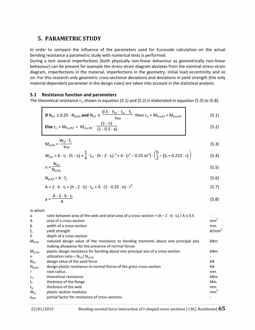
22/01/2015 Bending-normal force interaction of I-shaped cross-sections | I.M.J. Rombouts| 65
5. PARAMETRIC STUDY
In order to compare the influence of the parameters used for Eurocode calculation on the actual bending resistance a parametric study with numerical tests is performed. During a test several imperfections (both physically non-linear behaviour as geometrically non-linear behaviour) can be present for example the stress-strain diagram deviates from the nominal stress-strain diagram, imperfections in the material, imperfections in the geometry, initial load eccentricity and so on. For this research only geometric cross-sectional deviations and deviations in yield strength (the only material dependent parameter in the design rules) are taken into account in the statistical analysis.
5.1 Resistance function and parameters The theoretical resistance rt,i shown in equation (5.1) and (5.2) is elaborated in equation (5.3) to (5.8).
If NEd ≤ 0.25 ∙ Npl,Rd and NEd ≤ 0.5 ∙ hw ∙ tw ∙ fy
γM0 then rt,i = MN,y,Rd = Mpl,y,Rd (5.1)
Else rt,i = MN,y,Rd = Mpl,y,Rd ∙ (1 - n)
(1 - 0.5 ∙ a) (5.2)
Mpl,Rd = Wpl ∙ fy
γM0 (5.3)
Wpl,y = b ∙ tf ∙ (h - tf) + 14 ∙ tw ∙ (h - 2 ∙ tf)
2 + 4 ∙ (r2 – 0.25 πr2) ∙
h
2 – ( )tf + 0.223 ∙ r (5.4)
n = NEd
Npl,Rd (5.5)
Npl,Rd = A ∙ fy (5.6)
A = 2 ∙ b ∙ tf + (h - 2 ∙ tf) ∙ tw + 4 ∙ (1 - 0.25 ∙ π) ∙ r2 (5.7)
a = A - 2 ∙ b ∙ tf
A (5.8)
In which: a ratio between area of the web and total area of a cross-section = (A – 2 ∙ b ∙ tf) / A ≤ 0.5 - A area of a cross-section mm
2
b width of a cross-section mm fy yield strength N/mm
2
h depth of a cross-section MN,Rd reduced design value of the resistance to bending moments about one principal axis
making allowance for the presence of normal forces kNm
Mpl,Rd plastic design resistance for bending about one principal axis of a cross-section kNm n utilization ratio = NEd / Npl,Rd - NEd design value of the axial force kN Npl,Rd design plastic resistance to normal forces of the gross cross-section kN r root radius mm rt,i theoretical resistance kNm tf thickness of the flange Mm tw thickness of the web mm Wpl plastic section modulus mm
3
γM0 partial factor for resistance of cross-sections -
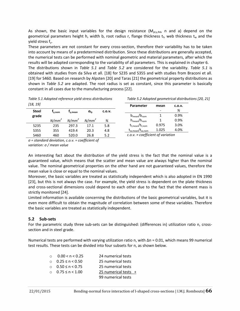
22/01/2015 Bending-normal force interaction of I-shaped cross-sections | I.M.J. Rombouts| 66
As shown, the basic input variables for the design resistance (Mpl,y,Rd, n and a) depend on the geometrical parameters height h, width b, root radius r, flange thickness tf, web thickness tw and the yield stress fy. These parameters are not constant for every cross-section, therefore their variability has to be taken into account by means of a predetermined distribution. Since these distributions are generally accepted, the numerical tests can be performed with nominal geometric and material parameters, after which the results will be adapted corresponding to the variability of all parameters. This is explained in chapter 6. The distributions shown in Table 5.1 and Table 5.2 are considered for the variability. Table 5.1 is obtained with studies from da Silva et all. [18] for S235 and S355 and with studies from Braconi et all. [19] for S460. Based on research by Alpsten [20] and Taras [21] the geometrical property distributions as shown in Table 5.2 are adapted. The root radius is set as constant, since this parameter is basically constant in all cases due to the manufacturing process [22].
Table 5.1 Adopted reference yield stress distributions
[18, 19]
Steel grade
fy,nom fy,mean σfy c.o.v.
N/mm2
N/mm2 N/mm
2 %
S235 235 297.3 17.1 5.8 S355 355 419.4 20.3 4.8 S460 460 520.0 26.8 5.2
σ = standard deviation, c.o.v. = coefficient of variation: σ / mean value
Table 5.2 Adopted geometrical distributions [20, 21]
Parameter mean c.o.v. -
%
bmean/bnom 1 0.9% hmean/hnom 1 0.9% tf,mean/tf,nom 0.975 3.0%
tw,mean/tw,nom 1.025 4.0%
c.o.v. = coefficient of variation
An interesting fact about the distribution of the yield stress is the fact that the nominal value is a guaranteed value, which means that the scatter and mean value are always higher than the nominal value. The nominal geometrical properties on the other hand are not guaranteed values, therefore the mean value is close or equal to the nominal values. Moreover, the basic variables are treated as statistically independent which is also adopted in EN 1990 [23], but this is not always the case. For example, the yield stress is dependent on the plate thickness and cross-sectional dimensions could depend to each other due to the fact that the element mass is strictly monitored [24]. Limited information is available concerning the distributions of the basic geometrical variables, but it is even more difficult to obtain the magnitude of correlation between some of these variables. Therefore the basic variables are treated as statistically independent.
5.2 Sub-sets For the parametric study three sub-sets can be distinguished: (differences in) utilization ratio n, cross-section and in steel grade. Numerical tests are performed with varying utilization ratio n, with ∆n = 0.01, which means 99 numerical test results. These tests can be divided into four subsets for n, as shown below.
o 0.00 < n < 0.25 24 numerical tests o 0.25 ≤ n < 0.50 25 numerical tests o 0.50 ≤ n < 0.75 25 numerical tests o 0.75 ≤ n < 1.00 25 numerical tests +
99 numerical tests

22/01/2015 Bending-normal force interaction of I-shaped cross-sections | I.M.J. Rombouts| 67
Figure 5.1 Graphic visualization of sub-sets n and number of nummerical tests
The other sub-set is defined by the type of cross-section to create cases with significant differences in Wpl,y, a and A. The first cross-section is a HEA240, since this research concentrates on this cross-section. Based on the Wpl,y, factor a and A, other I-shaped cross-sections are chosen, which leads to the subsets as shown below. This leads to a total population of 396 numerical tests.
o HEA240 - 99 numerical tests o HEM400 similar a 99 numerical tests o IPE330 similar Wpl,y 99 numerical tests o HEB200 similar A, a 99 numerical tests +
396 numerical tests Table 5.3 summarizes the most important parameters of the HEM-, IPE- and HEB cross-section compared to the HEA cross-section. As shown, the HEM400 section has a significant deviation in plastic section modulus Wpl,y and cross-section A, but the ratio between the area of the web and the total area is similar to the HEA240 cross-section. The plastic section modulus of the IPE330 cross-section is similar to that of the HEA240 cross-section. Figure 5.2 shows the representation of the cross-sectional sub-set.
Table 5.3 Cross-sections with their parameters relative to a HEA240 cross-section
Wpl,y A a % % %
HEA240 100.00 100.00 100.00 HEB200 82.29 101.62 92.50 HEM400 748.11 423.99 98.31 IPE330 108.02 81.84 164.65
24
25
25
25

22/01/2015 Bending-normal force interaction of I-shaped cross-sections | I.M.J. Rombouts| 68
Figure 5.2 Sub-set cross-sections
According to the Eurocode [1] and the exact caulation, the factor of a is the most determining factor for the My-N interaction curve, as shown in Figure 5.3. The IPE330 cross-section dimensionless curve deviates the most, which represents the high value of a compared to the rest. The high plastic section modulus and cross-section of the HEM400 cross-section does not significantly affect the curve. The HEB200 and HEA240 curves are logically similar.
Figure 5.3 My-N interaction of different cross-sections: exact versus Eurocode [1]
The last sub-set concerns steel grades. Until now this research project was all about specimens in steel grade S235, but S355 and S460 are steel grades which are often used nowadays. The design formulas on M-N interaction in the Eurocode [1] describe a linear relation between the yield stress (the only material dependent variable) and the reduced plastic bending moment resistance.
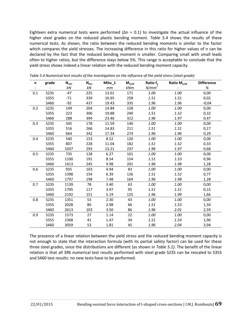
22/01/2015 Bending-normal force interaction of I-shaped cross-sections | I.M.J. Rombouts| 69
Eighteen extra numerical tests were performed (∆n = 0.1) to investigate the actual influence of the higher steel grades on the reduced plastic bending moment. Table 5.4 shows the results of these numerical tests. As shown, the ratio between the reduced bending moments is similar to the factor which compares the yield stresses. The increasing difference in this ratio for higher values of n can be declared by the fact that the reduced bending moment is smaller. Comparing small with small leads often to higher ratios, but the difference stays below 5%. This range is acceptable to conclude that the yield stress shows indeed a linear relation with the reduced bending moment capacity.
Table 5.4 Numerical test results of the investigation on the influence of the yield stress (steel grade)
n grade Ncen Necc Mitu_1 My,Ed Ratio fy Ratio My,Ed Difference - - kN kN mm kNm N/mm
2 - %
0.1 S235 -47 225 13.01 171 1.00 1.00 0,00
S355 -71 339 16.95 258 1.51 1.51 0,02
S460 -92 437 19.43 335 1.96 1.96 -0,04
0.2 S235 149 204 14.84 158 1.00 1.00 0,00
S355 223 306 19.88 240 1.51 1.52 0,32
S460 288 394 23.46 312 1.96 1.97 0,47
0.3 S235 345 178 11.59 140 1.00 1.00 0,00
S355 516 266 14.83 211 1.51 1.51 0,17
S460 664 342 17.34 274 1.96 1.96 0,29
0.4 S235 540 153 8.52 120 1.00 1.00 0,00
S355 807 228 11.04 182 1.51 1.52 0,33
S460 1037 293 13.21 237 1.96 1.97 0,68
0.5 S235 735 128 6.27 101 1.00 1.00 0,00
S355 1100 191 8.54 154 1.51 1.53 0,96
S460 1413 245 9.98 201 1.96 1.98 1,28
0.6 S235 935 103 4.94 83 1.00 1.00 0,00
S355 1398 154 6.39 126 1.51 1.52 0,77
S460 1797 198 7.48 164 1.96 1.98 1,28
0.7 S235 1139 78 3.40 63 1.00 1.00 0,00
S355 1705 117 3.97 95 1.51 1.51 0,15
S460 2192 151 5.19 125 1.96 1.99 1,66
0.8 S235 1351 53 2.30 43 1.00 1.00 0,00
S355 2028 80 2.98 66 1.51 1.53 1,50
S460 2613 103 3.50 86 1.96 2.01 2,59
0.9 S235 1573 27 1.14 22 1.00 1.00 0,00
S355 2368 41 1.47 34 1.51 1.54 1,96
S460 3059 53 1.81 45 1.96 2.04 3,94
The presence of a linear relation between the yield stress and the reduced bending moment capacity is not enough to state that the interaction formula (with its partial safety factor) can be used for these three steel grades, since the distributions are different (as shown in Table 5.1). The benefit of the linear relation is that all 396 numerical test results performed with steel grade S235 can be rescaled to S355 and S460 test results: no new tests have to be performed.

22/01/2015 Bending-normal force interaction of I-shaped cross-sections | I.M.J. Rombouts| 70
5.3 Numerical test results Figure 5.4 and Figure 5.5 show the numerical test results in the corresponding My-N interaction diagram compared with the Eurocode design rules and the exact solution. As shown, the numerical test results are similar with the exact solution for small values of n, while the Eurocode gives an unconservative prediction. For utilization ratios between roughly 0.4 and 0.8, the numerical test results are more in line with the Eurocode [1].
Figure 5.4 HEA240 numerical test results
Figure 5.5 HEB200 numerical test results
Figure 5.6 and Figure 5.7 show the ratio between the experimental (numerical) and theoretical (Eurocode) test results. The dip around n = 0.1 represents the deviation of the numerical test results from the Eurocode line in the figures above. The high ratios for high values of n over exaggerated the difference, since it compares two small values.
Figure 5.6 Ratio re / rt,EC3 HEA240
Figure 5.7 Ratio re / rt,EC3 HEB200

22/01/2015 Bending-normal force interaction of I-shaped cross-sections | I.M.J. Rombouts| 71
Figure 5.8 to Figure 5.11 show the numerical test results for the IPE330 and HEM400 cross-section. As shown, the IPE330 cross-section is similar to the exact solution, which results in a larger gap between Eurocode and numerical tests and a lower ratio re / rt,EC3 than the first two cross-sections, due to the high value of the factor a. The HEM400 cross-section deviates more from the exact solution, particularly for n < 0.5.
Figure 5.8 IPE330 numerical test results
Figure 5.9 Ratio re / rt,EC3 IPE330
Figure 5.10 HEM400 numerical test results
Figure 5.11 Ratio re / rt,EC3 HEM400
5.4 Summary, discussion and conclusions This paragraph briefly summarizes chapter 5 and describes the main conclusions. 5.4.1 Summary In order to compare the influence of the parameters used for Eurocode calculations on the actual bending resistance a parametric study with numerical tests is performed. For this research geometric
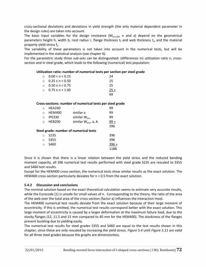
22/01/2015 Bending-normal force interaction of I-shaped cross-sections | I.M.J. Rombouts| 72
cross-sectional deviations and deviations in yield strength (the only material dependent parameter in the design rules) are taken into account. The basic input variables for the design resistance (Mpl,y,Rd, n and a) depend on the geometrical parameters height h, width b, root radius r, flange thickness tf and web thickness tw and the material property yield stress fy. The variability of these parameters is not taken into account in the numerical tests, but will be implemented in the statistical analysis (see chapter 6). For the parametric study three sub-sets can be distinguished: (differences in) utilization ratio n, cross-section and in steel grade, which leads to the following (numerical) test population:
Utilization ratio: number of numerical tests per section per steel grade o 0.00 < n < 0.25 24 o 0.25 ≤ n < 0.50 25 o 0.50 ≤ n < 0.75 25 o 0.75 ≤ n < 1.00 25 +
99 Cross-sections: number of numerical tests per steel grade
o HEA240 - 99 o HEM400 similar a 99 o IPE330 similar Wpl,y 99 o HEB200 similar Wpl,y, a, A 99 +
396 Steel grade: number of numerical tests
o S235 396 o S355 396 o S460 396 +
1188 Since it is shown that there is a linear relation between the yield stress and the reduced bending moment capacity, all 396 numerical test results performed with steel grade S235 are rescaled to S355 and S460 test results. Except for the HEM400 cross-section, the numerical tests show similar results as the exact solution. The HEM400 cross-section particularly deviates for n < 0.5 from the exact solution. 5.4.2 Discussion and conclusions The nominal solution based on the exact theoretical calculation seems to estimate very accurate results, while the Eurocode [1] is unsafe for small values of n. Corresponding to the theory, the ratio of the area of the web over the total area of the cross-section (factor a) influences the interaction most. The HEM400 numerical test results deviate from the exact solution because of their large moment of eccentricity. If this is omitted, the numerical test results correspond better with the exact solution. This large moment of eccentricity is caused by a larger deformation at the maximum failure load, due to the stocky flanges (12, 11.5 and 15 mm compared to 40 mm for the HEM400). The stockiness of the flanges prevent buckling due to yielding easily. The numerical test results for steel grades S355 and S460 are equal to the test results shown in this chapter, since these are only rescaled by increasing the yield stress. Figure 5.4 until Figure 5.11 are valid for all three steel grades because the graphs are dimensionless.

22/01/2015 Bending-normal force interaction of I-shaped cross-sections | I.M.J. Rombouts| 73
6. STATISTICAL EVALUATION
This chapter describes the statistical evaluation of 1188 nominal numerical test results. The five variables for the basis of the design formula (b, h, tw, tf, fy) will be considered as independent variables. After discounting for the error in the resistance function and the variability of these variables, a partial safety factor will be calculated and compared to the target value of γM0 = 1.00.
6.1 Methodology The first step in the statistical evaluation according to Annex D of EN 1990 [23] is to calculate the mean value of the correction factor b, as shown in equation (6.1). This factor is a global value for a subset, it represents the accuracy of the resistance function and should therefore not strongly diverge from unity.
b =
i = 1
n re,i ∙ rt,i
i = 1
n rt,i
2
(6.1)
With: b Correction factor - re,i Experimental (numerical in this case) resistance value for specimen i kNm rt,i Theoretical (Eurocode [1] in this case) resistance value for specimen i kNm n Number of numerical tests -
The second step is to determine the error term (equation (6.2)) and the coefficient of variation of the error term Vδ, which is again a global value for the subset. The calculation of this factor is shown in equation (6.3) to (6.5).
δi = re,i
b ∙ rt,i (error term) (6.2)
∆i = ln(δi) (6.3)
s∆2 =
1n-1 ∙
i = 1
n (∆i - ∆mean)2 (6.4)
Vδ = exp(s∆2) - 1 (6.5)
The third step is to determine the coefficient of variation of the basic input variables Vrt with the pre-information summarized in chapter 5. Since the resistance function is not a simple product function, Vrt is obtained for each specimen as shown in equation (6.6). The partial derivates are determined by means of a numerical iterative process, according to the flow chart shown in Annex 11.21.
Vrt,i 2 =
1rt,i ∙ (Xm) 2 ∙
j = 1
k
drt,i (Xj)
dXj ∙ σj (6.6)
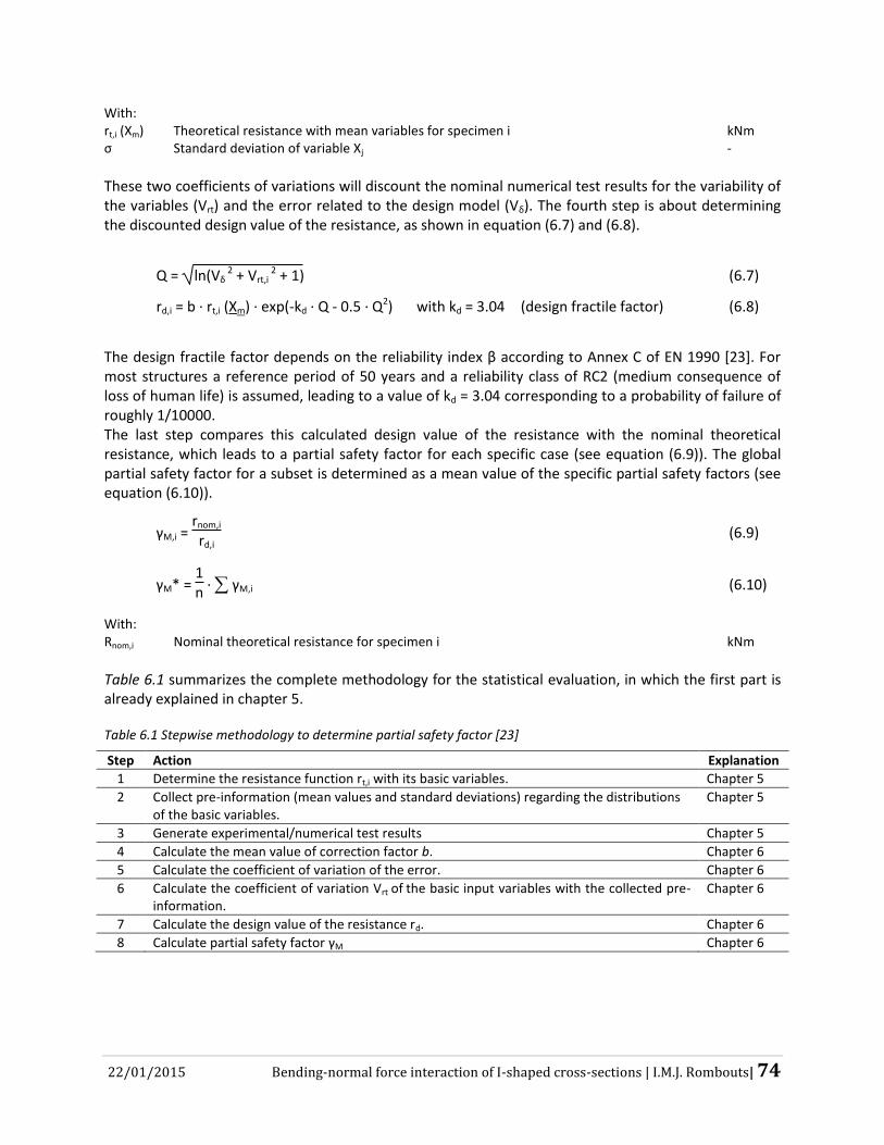
22/01/2015 Bending-normal force interaction of I-shaped cross-sections | I.M.J. Rombouts| 74
With: rt,i (Xm) Theoretical resistance with mean variables for specimen i kNm σ Standard deviation of variable Xj -
These two coefficients of variations will discount the nominal numerical test results for the variability of the variables (Vrt) and the error related to the design model (Vδ). The fourth step is about determining the discounted design value of the resistance, as shown in equation (6.7) and (6.8).
Q = ln(Vδ 2 + Vrt,i
2 + 1) (6.7)
rd,i = b ∙ rt,i (Xm) ∙ exp(-kd ∙ Q - 0.5 ∙ Q2) with kd = 3.04 (design fractile factor) (6.8)
The design fractile factor depends on the reliability index β according to Annex C of EN 1990 [23]. For most structures a reference period of 50 years and a reliability class of RC2 (medium consequence of loss of human life) is assumed, leading to a value of kd = 3.04 corresponding to a probability of failure of roughly 1/10000. The last step compares this calculated design value of the resistance with the nominal theoretical resistance, which leads to a partial safety factor for each specific case (see equation (6.9)). The global partial safety factor for a subset is determined as a mean value of the specific partial safety factors (see equation (6.10)).
γM,i = rnom,i
rd,i (6.9)
γM* = 1n ∙ γM,i (6.10)
With: Rnom,i Nominal theoretical resistance for specimen i kNm
Table 6.1 summarizes the complete methodology for the statistical evaluation, in which the first part is already explained in chapter 5.
Table 6.1 Stepwise methodology to determine partial safety factor [23]
Step Action Explanation
1 Determine the resistance function rt,i with its basic variables. Chapter 5
2 Collect pre-information (mean values and standard deviations) regarding the distributions of the basic variables.
Chapter 5
3 Generate experimental/numerical test results Chapter 5
4 Calculate the mean value of correction factor b. Chapter 6
5 Calculate the coefficient of variation of the error. Chapter 6
6 Calculate the coefficient of variation Vrt of the basic input variables with the collected pre-information.
Chapter 6
7 Calculate the design value of the resistance rd. Chapter 6
8 Calculate partial safety factor γM Chapter 6
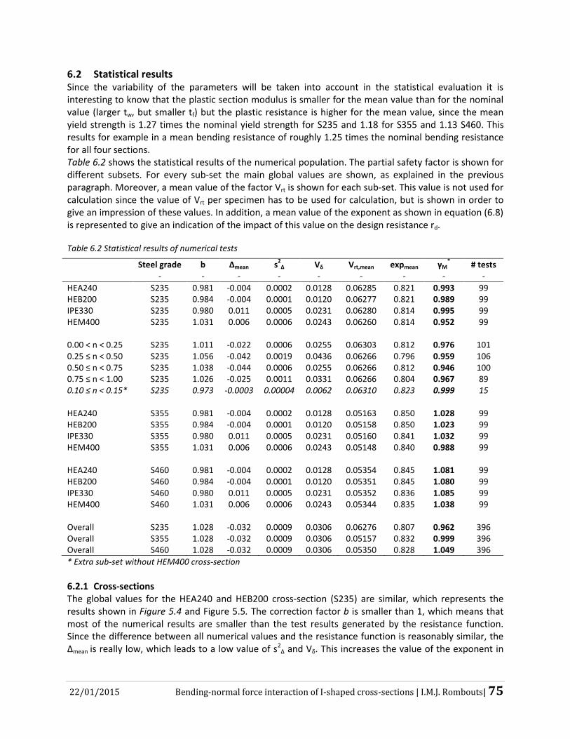
22/01/2015 Bending-normal force interaction of I-shaped cross-sections | I.M.J. Rombouts| 75
6.2 Statistical results Since the variability of the parameters will be taken into account in the statistical evaluation it is interesting to know that the plastic section modulus is smaller for the mean value than for the nominal value (larger tw, but smaller tf) but the plastic resistance is higher for the mean value, since the mean yield strength is 1.27 times the nominal yield strength for S235 and 1.18 for S355 and 1.13 S460. This results for example in a mean bending resistance of roughly 1.25 times the nominal bending resistance for all four sections. Table 6.2 shows the statistical results of the numerical population. The partial safety factor is shown for different subsets. For every sub-set the main global values are shown, as explained in the previous paragraph. Moreover, a mean value of the factor Vrt is shown for each sub-set. This value is not used for calculation since the value of Vrt per specimen has to be used for calculation, but is shown in order to give an impression of these values. In addition, a mean value of the exponent as shown in equation (6.8) is represented to give an indication of the impact of this value on the design resistance rd.
Table 6.2 Statistical results of numerical tests
Steel grade b ∆mean s2
∆ Vδ Vrt,mean expmean γM*
# tests - - - - - - - - -
HEA240 S235 0.981 -0.004 0.0002 0.0128 0.06285 0.821 0.993 99 HEB200 S235 0.984 -0.004 0.0001 0.0120 0.06277 0.821 0.989 99 IPE330 S235 0.980 0.011 0.0005 0.0231 0.06280 0.814 0.995 99 HEM400 S235 1.031 0.006 0.0006 0.0243 0.06260 0.814 0.952 99 0.00 < n < 0.25 S235 1.011 -0.022 0.0006 0.0255 0.06303 0.812 0.976 101 0.25 ≤ n < 0.50 S235 1.056 -0.042 0.0019 0.0436 0.06266 0.796 0.959 106 0.50 ≤ n < 0.75 S235 1.038 -0.044 0.0006 0.0255 0.06266 0.812 0.946 100 0.75 ≤ n < 1.00 S235 1.026 -0.025 0.0011 0.0331 0.06266 0.804 0.967 89 0.10 ≤ n < 0.15* S235 0.973 -0.0003 0.00004 0.0062 0.06310 0.823 0.999 15 HEA240 S355 0.981 -0.004 0.0002 0.0128 0.05163 0.850 1.028 99 HEB200 S355 0.984 -0.004 0.0001 0.0120 0.05158 0.850 1.023 99 IPE330 S355 0.980 0.011 0.0005 0.0231 0.05160 0.841 1.032 99 HEM400 S355 1.031 0.006 0.0006 0.0243 0.05148 0.840 0.988 99 HEA240 S460 0.981 -0.004 0.0002 0.0128 0.05354 0.845 1.081 99 HEB200 S460 0.984 -0.004 0.0001 0.0120 0.05351 0.845 1.080 99 IPE330 S460 0.980 0.011 0.0005 0.0231 0.05352 0.836 1.085 99 HEM400 S460 1.031 0.006 0.0006 0.0243 0.05344 0.835 1.038 99 Overall S235 1.028 -0.032 0.0009 0.0306 0.06276 0.807 0.962 396 Overall S355 1.028 -0.032 0.0009 0.0306 0.05157 0.832 0.999 396 Overall S460 1.028 -0.032 0.0009 0.0306 0.05350 0.828 1.049 396
* Extra sub-set without HEM400 cross-section
6.2.1 Cross-sections The global values for the HEA240 and HEB200 cross-section (S235) are similar, which represents the results shown in Figure 5.4 and Figure 5.5. The correction factor b is smaller than 1, which means that most of the numerical results are smaller than the test results generated by the resistance function. Since the difference between all numerical values and the resistance function is reasonably similar, the ∆mean is really low, which leads to a low value of s2
∆ and Vδ. This increases the value of the exponent in
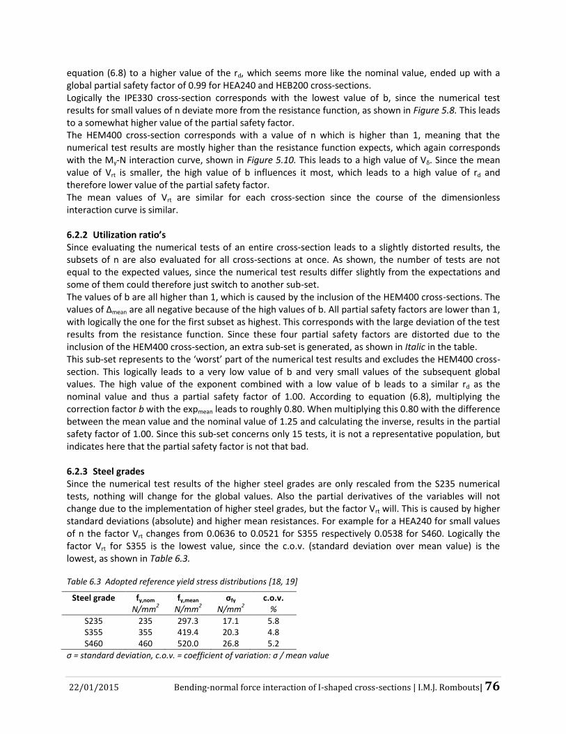
22/01/2015 Bending-normal force interaction of I-shaped cross-sections | I.M.J. Rombouts| 76
equation (6.8) to a higher value of the rd, which seems more like the nominal value, ended up with a global partial safety factor of 0.99 for HEA240 and HEB200 cross-sections. Logically the IPE330 cross-section corresponds with the lowest value of b, since the numerical test results for small values of n deviate more from the resistance function, as shown in Figure 5.8. This leads to a somewhat higher value of the partial safety factor. The HEM400 cross-section corresponds with a value of n which is higher than 1, meaning that the numerical test results are mostly higher than the resistance function expects, which again corresponds with the My-N interaction curve, shown in Figure 5.10. This leads to a high value of Vδ. Since the mean value of Vrt is smaller, the high value of b influences it most, which leads to a high value of rd and therefore lower value of the partial safety factor. The mean values of Vrt are similar for each cross-section since the course of the dimensionless interaction curve is similar. 6.2.2 Utilization ratio’s Since evaluating the numerical tests of an entire cross-section leads to a slightly distorted results, the subsets of n are also evaluated for all cross-sections at once. As shown, the number of tests are not equal to the expected values, since the numerical test results differ slightly from the expectations and some of them could therefore just switch to another sub-set. The values of b are all higher than 1, which is caused by the inclusion of the HEM400 cross-sections. The values of ∆mean are all negative because of the high values of b. All partial safety factors are lower than 1, with logically the one for the first subset as highest. This corresponds with the large deviation of the test results from the resistance function. Since these four partial safety factors are distorted due to the inclusion of the HEM400 cross-section, an extra sub-set is generated, as shown in Italic in the table. This sub-set represents to the ‘worst’ part of the numerical test results and excludes the HEM400 cross-section. This logically leads to a very low value of b and very small values of the subsequent global values. The high value of the exponent combined with a low value of b leads to a similar rd as the nominal value and thus a partial safety factor of 1.00. According to equation (6.8), multiplying the correction factor b with the expmean leads to roughly 0.80. When multiplying this 0.80 with the difference between the mean value and the nominal value of 1.25 and calculating the inverse, results in the partial safety factor of 1.00. Since this sub-set concerns only 15 tests, it is not a representative population, but indicates here that the partial safety factor is not that bad. 6.2.3 Steel grades Since the numerical test results of the higher steel grades are only rescaled from the S235 numerical tests, nothing will change for the global values. Also the partial derivatives of the variables will not change due to the implementation of higher steel grades, but the factor Vrt will. This is caused by higher standard deviations (absolute) and higher mean resistances. For example for a HEA240 for small values of n the factor Vrt changes from 0.0636 to 0.0521 for S355 respectively 0.0538 for S460. Logically the factor Vrt for S355 is the lowest value, since the c.o.v. (standard deviation over mean value) is the lowest, as shown in Table 6.3.
Table 6.3 Adopted reference yield stress distributions [18, 19]
Steel grade fy,nom fy,mean σfy c.o.v. N/mm
2 N/mm
2 N/mm
2 %
S235 235 297.3 17.1 5.8 S355 355 419.4 20.3 4.8 S460 460 520.0 26.8 5.2
σ = standard deviation, c.o.v. = coefficient of variation: σ / mean value
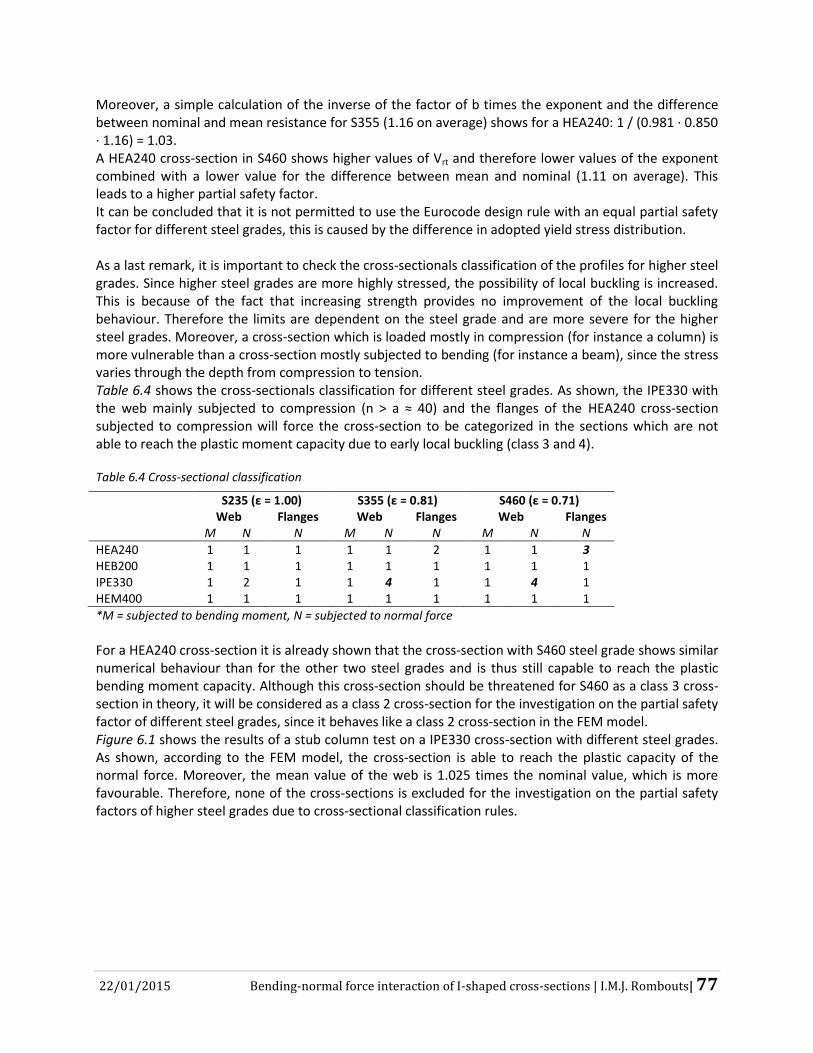
22/01/2015 Bending-normal force interaction of I-shaped cross-sections | I.M.J. Rombouts| 77
Moreover, a simple calculation of the inverse of the factor of b times the exponent and the difference between nominal and mean resistance for S355 (1.16 on average) shows for a HEA240: 1 / (0.981 ∙ 0.850 ∙ 1.16) = 1.03. A HEA240 cross-section in S460 shows higher values of Vrt and therefore lower values of the exponent combined with a lower value for the difference between mean and nominal (1.11 on average). This leads to a higher partial safety factor. It can be concluded that it is not permitted to use the Eurocode design rule with an equal partial safety factor for different steel grades, this is caused by the difference in adopted yield stress distribution. As a last remark, it is important to check the cross-sectionals classification of the profiles for higher steel grades. Since higher steel grades are more highly stressed, the possibility of local buckling is increased. This is because of the fact that increasing strength provides no improvement of the local buckling behaviour. Therefore the limits are dependent on the steel grade and are more severe for the higher steel grades. Moreover, a cross-section which is loaded mostly in compression (for instance a column) is more vulnerable than a cross-section mostly subjected to bending (for instance a beam), since the stress varies through the depth from compression to tension. Table 6.4 shows the cross-sectionals classification for different steel grades. As shown, the IPE330 with the web mainly subjected to compression (n > a ≈ 40) and the flanges of the HEA240 cross-section subjected to compression will force the cross-section to be categorized in the sections which are not able to reach the plastic moment capacity due to early local buckling (class 3 and 4).
Table 6.4 Cross-sectional classification
S235 (ε = 1.00) S355 (ε = 0.81) S460 (ε = 0.71) Web Flanges Web Flanges Web Flanges M N N M N N M N N
HEA240 1 1 1 1 1 2 1 1 3 HEB200 1 1 1 1 1 1 1 1 1 IPE330 1 2 1 1 4 1 1 4 1 HEM400 1 1 1 1 1 1 1 1 1
*M = subjected to bending moment, N = subjected to normal force
For a HEA240 cross-section it is already shown that the cross-section with S460 steel grade shows similar numerical behaviour than for the other two steel grades and is thus still capable to reach the plastic bending moment capacity. Although this cross-section should be threatened for S460 as a class 3 cross-section in theory, it will be considered as a class 2 cross-section for the investigation on the partial safety factor of different steel grades, since it behaves like a class 2 cross-section in the FEM model. Figure 6.1 shows the results of a stub column test on a IPE330 cross-section with different steel grades. As shown, according to the FEM model, the cross-section is able to reach the plastic capacity of the normal force. Moreover, the mean value of the web is 1.025 times the nominal value, which is more favourable. Therefore, none of the cross-sections is excluded for the investigation on the partial safety factors of higher steel grades due to cross-sectional classification rules.

22/01/2015 Bending-normal force interaction of I-shaped cross-sections | I.M.J. Rombouts| 78
Figure 6.1 Force-deformation diagram of a IPE330 stub column
6.2.4 Overall At last, all 396 numerical test results per steel grade are statistically evaluated. The partial safety factor for steel grade S235 is 0.96 (apparently influenced due to the HEM400 test results and the high c.o.v.). For steel grade S355, the partial safety factor is 1.00. However, the partial safety factor for steel grade S460 cross-sections rises to 1.049, which can be questioned to round to 1.00 or 1.10. In fact, the calculated design resistance should be multiplied with 1.049 to reach the target value of γM
* = 1.00. To create a higher design resistance, a lower factor of kd is needed in equation (6.8). On
average kd = 2.27 suffices, corresponding to a probability of failure of roughly 1/1000. This means that the probability of failure is increased tenfold when the partial safety factor of 1.00 is maintained. 6.2.5 Coefficient of variation of the error term for the FEM model (Vδ,FEM) As shown in Figure 4.16, the error related to the difference between the FEM model and the experimental test results is small, but this can be included in the statistical evaluation by means of an extra coefficient of variation of the error term Vδ,FEM. The calculation of this extra coefficient of variation is similar as mentioned earlier. The global results are shown in equation (6.11) to (6.14). The inclusion of
this small extra parameter leads for example for the HEA240 overall set to Vδ,total = 0.03062 + 0.00882 = 0.0318 (see equation 6.15) instead of Vδ = 0.306 (increase of ≈ 4.0%).
b =
i = 1
n re,i ∙ rt,i,FEM
i = 1
n rt,i
2
= 1.00455 (6.11)

22/01/2015 Bending-normal force interaction of I-shaped cross-sections | I.M.J. Rombouts| 79
∆i = ln(δi) = -0.01039 (6.12)
s∆2 =
1n-1 ∙
i = 1
n (∆i - ∆mean)2 = 0.00008 (6.13)
Vδ,FEM = exp(s∆2) - 1 = 0.00884 (6.14)
V2δ,total = V2
δ + V2δ,FEM (6.15)
For the subset mentioned above, the factor of Q increases with 0.74%, which does not lead to a significant increase in the partial safety factor. Therefore, this extra factor will be omitted.
6.3 Summary, discussion and conclusions This paragraph briefly summarizes chapter 6 and describes the main conclusions. 6.3.1 Summary The statistical evaluation of 1188 numerical tests results performed with the FEM model which was validated by means of the experimental tests considers the five variables for the base of the design formula (b, h, tw, tf, fy) as independent variables. Table 6.5 summarizes the complete methodology for the statistical evaluation, in which the first part is already explained in chapter 5. In basis, the numerical test results will be discounted for the error of the resistance function and the variability of the parameters.
Table 6.5 Stepwise methodology to determine partial safety factor [23]
Step Action Explanation
1 Determine the resistance function rt,i with its basic variables. Chapter 5
2 Collect pre-information (mean values and standard deviations) regarding the distributions of the basic variables.
Chapter 5
3 Generate experimental/numerical test results Chapter 5
4 Calculate the mean value of correction factor b. Chapter 6
5 Calculate the coefficient of variation of the error. Chapter 6
6 Calculate the coefficient of variation Vrt of the basic input variables with the collected pre-information.
Chapter 6
7 Calculate the design value of the resistance rd. Chapter 6
8 Calculate partial safety factor γM Chapter 6
A summary of the statistical evaluation is shown in Table 6.6. As shown, the HEA240, IPE330 and HEB200 show roughly safe results (can be rounded off to 1.00) for S235 and S355 while the partial safety factor for HEM400 cross-section could be noted as conservative for S235. This is caused by the high numerical test results due to the larger moment of eccentricity due to stocky flanges. The partial safety factors should be higher for higher steel grades, caused by a lower c.o.v. and difference between mean and nominal resistance.
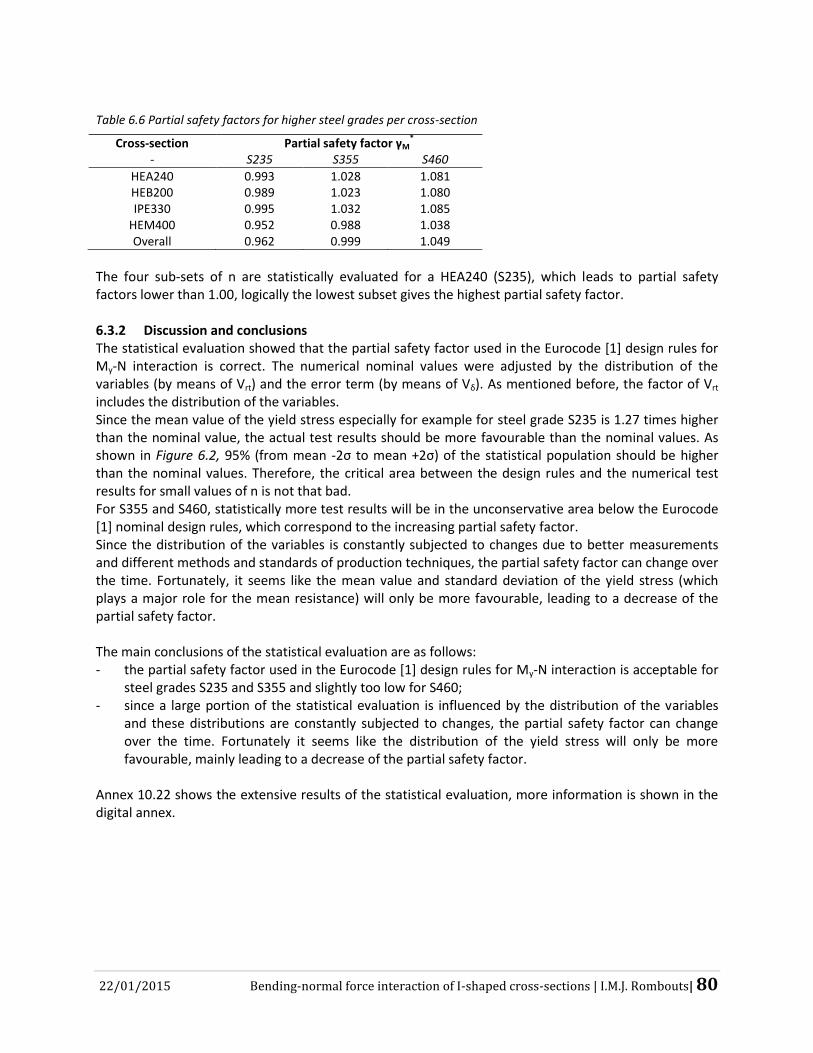
22/01/2015 Bending-normal force interaction of I-shaped cross-sections | I.M.J. Rombouts| 80
Table 6.6 Partial safety factors for higher steel grades per cross-section
Cross-section Partial safety factor γM*
- S235 S355 S460
HEA240 0.993 1.028 1.081 HEB200 0.989 1.023 1.080 IPE330 0.995 1.032 1.085
HEM400 0.952 0.988 1.038 Overall 0.962 0.999 1.049
The four sub-sets of n are statistically evaluated for a HEA240 (S235), which leads to partial safety factors lower than 1.00, logically the lowest subset gives the highest partial safety factor. 6.3.2 Discussion and conclusions The statistical evaluation showed that the partial safety factor used in the Eurocode [1] design rules for My-N interaction is correct. The numerical nominal values were adjusted by the distribution of the variables (by means of Vrt) and the error term (by means of Vδ). As mentioned before, the factor of Vrt includes the distribution of the variables. Since the mean value of the yield stress especially for example for steel grade S235 is 1.27 times higher than the nominal value, the actual test results should be more favourable than the nominal values. As shown in Figure 6.2, 95% (from mean -2σ to mean +2σ) of the statistical population should be higher than the nominal values. Therefore, the critical area between the design rules and the numerical test results for small values of n is not that bad. For S355 and S460, statistically more test results will be in the unconservative area below the Eurocode [1] nominal design rules, which correspond to the increasing partial safety factor. Since the distribution of the variables is constantly subjected to changes due to better measurements and different methods and standards of production techniques, the partial safety factor can change over the time. Fortunately, it seems like the mean value and standard deviation of the yield stress (which plays a major role for the mean resistance) will only be more favourable, leading to a decrease of the partial safety factor. The main conclusions of the statistical evaluation are as follows: - the partial safety factor used in the Eurocode [1] design rules for My-N interaction is acceptable for
steel grades S235 and S355 and slightly too low for S460; - since a large portion of the statistical evaluation is influenced by the distribution of the variables
and these distributions are constantly subjected to changes, the partial safety factor can change over the time. Fortunately it seems like the distribution of the yield stress will only be more favourable, mainly leading to a decrease of the partial safety factor.
Annex 10.22 shows the extensive results of the statistical evaluation, more information is shown in the digital annex.

22/01/2015 Bending-normal force interaction of I-shaped cross-sections | I.M.J. Rombouts| 81
Figure 6.2 My-N interaction of HEB200: nominal, mean, and standard deviation for three steel grades

22/01/2015 Bending-normal force interaction of I-shaped cross-sections | I.M.J. Rombouts| 82
7. BRIEF ADDITIONAL STUDIES
The subject of M-N interaction has a lot more interesting aspects which are not investigated before, three of these subjects are investigated briefly during this project and described in this chapter.
7.1 Strain-hardening All numerical test results were performed with elastic-perfect plastic material behaviour (bilinear) since the implementation of the experimental curves of strain hardening did not lead to corresponding numerical results (an increasing plastic branch after a nearly horizontal plastic plateau). Nine extra numerical tests were performed to investigate the influence of including the curve of strain hardening in the material model. An idealized stress-strain curve according to EN-100025 [25] and EN-10225 [26] is used to implement the ‘nominal strain hardening’, see Figure 7.1.
Figure 7.1 Stress-strain curves of S235: bilinear / including strain hardening
Figure 7.2 shows the force deformation diagram for a HEA240 with utilization ratio n ≈ 0.4. As shown, similar failure loads are reached, the only difference is the deformation Mitu_1 at failure, caused by the predefined difference in strain at yielding.
Figure 7.2 Force-deformation diagram: bilinear / including strain hardening (HEA240)

22/01/2015 Bending-normal force interaction of I-shaped cross-sections | I.M.J. Rombouts| 83
Table 7.1 shows the numerical tests result compared to equal numerical tests with bilinear material behaviour. The representation of these test results is shown in a My-N interaction diagram in Figure 7.3. As shown, the differences are minimal, the failure loads are similar for n < 0.5, but the extra moment caused by eccentricity at mid-height Mitu_1 makes the difference for the My-N interaction diagram. Due to higher normal forces and lower bending moments, the deformation is smaller for larger values of n, which means that the material model including strain hardening reaches a lower failure load (less strain, lower stress, see Figure 7.1).
Table 7.1 Numerical test results: with and without strain hardeningHEA240
WITHOUT STRAIN HARDENING INCLUDING STRAIN HARDENING Ncen Necc NEd Mitu_1 My,Ed n m* Ncen Necc NEd Mitu_1 My,Ed n m* kN kN kN mm kNm - - kN kN kN mm kNm - -
-47 225 178 12,64 171 0,10 0,98 -47 224 177 23,90 172 0,10 0,98 149 204 353 15,21 159 0,20 0,91 149 204 353 15,39 159 0,20 0,91 346 178 524 13,78 141 0,29 0,80 347 179 526 17,43 143 0,29 0,82 540 153 692 8,72 120 0,38 0,69 540 152 692 14,53 124 0,38 0,71 735 128 863 6,28 101 0,48 0,58 732 127 859 10,91 105 0,48 0,60 934 103 1038 4,76 82 0,57 0,47 922 102 1024 9,50 86 0,57 0,49
1139 78 1217 3,33 63 0,67 0,36 1114 77 1191 8,92 68 0,66 0,39 1351 53 1404 2,31 43 0,78 0,25 1309 51 1360 8,18 50 0,75 0,28 1573 27 1600 1,14 22 0,89 0,13 1506 26 1532 7,52 31 0,85 0,18
* m = My,Ed / My,pl,Rd
Figure 7.4 My-N interaction HEA240 including strain hardening
Test results based on the inclusion of nominal strain hardening do not differ much from nominal bilinear material behaviour, while for the validation of the experimental tests this difference is of importance, this can be explained by the inclusion of the ‘steep’ curves of strain hardening nearby the roots. As
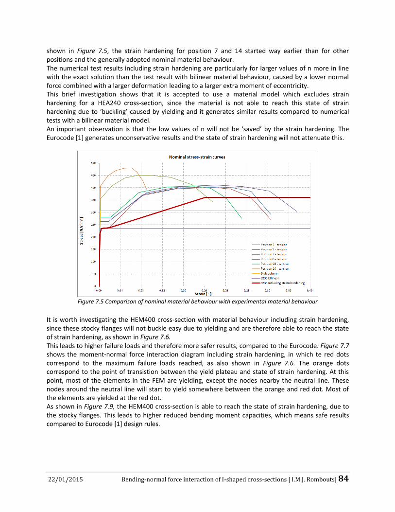
22/01/2015 Bending-normal force interaction of I-shaped cross-sections | I.M.J. Rombouts| 84
shown in Figure 7.5, the strain hardening for position 7 and 14 started way earlier than for other positions and the generally adopted nominal material behaviour. The numerical test results including strain hardening are particularly for larger values of n more in line with the exact solution than the test result with bilinear material behaviour, caused by a lower normal force combined with a larger deformation leading to a larger extra moment of eccentricity. This brief investigation shows that it is accepted to use a material model which excludes strain hardening for a HEA240 cross-section, since the material is not able to reach this state of strain hardening due to ‘buckling’ caused by yielding and it generates similar results compared to numerical tests with a bilinear material model. An important observation is that the low values of n will not be ‘saved’ by the strain hardening. The Eurocode [1] generates unconservative results and the state of strain hardening will not attenuate this.
Figure 7.5 Comparison of nominal material behaviour with experimental material behaviour
It is worth investigating the HEM400 cross-section with material behaviour including strain hardening, since these stocky flanges will not buckle easy due to yielding and are therefore able to reach the state of strain hardening, as shown in Figure 7.6. This leads to higher failure loads and therefore more safer results, compared to the Eurocode. Figure 7.7 shows the moment-normal force interaction diagram including strain hardening, in which te red dots correspond to the maximum failure loads reached, as also shown in Figure 7.6. The orange dots correspond to the point of transistion between the yield plateau and state of strain hardening. At this point, most of the elements in the FEM are yielding, except the nodes nearby the neutral line. These nodes around the neutral line will start to yield somewhere between the orange and red dot. Most of the elements are yielded at the red dot. As shown in Figure 7.9, the HEM400 cross-section is able to reach the state of strain hardening, due to the stocky flanges. This leads to higher reduced bending moment capacities, which means safe results compared to Eurocode [1] design rules.
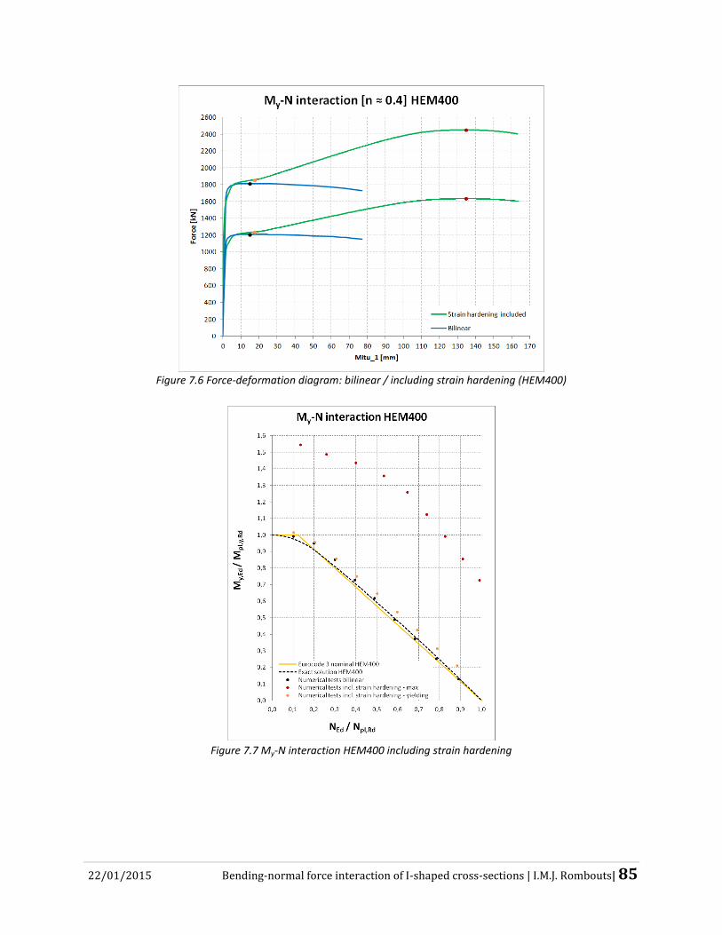
22/01/2015 Bending-normal force interaction of I-shaped cross-sections | I.M.J. Rombouts| 85
Figure 7.6 Force-deformation diagram: bilinear / including strain hardening (HEM400)
Figure 7.7 My-N interaction HEM400 including strain hardening
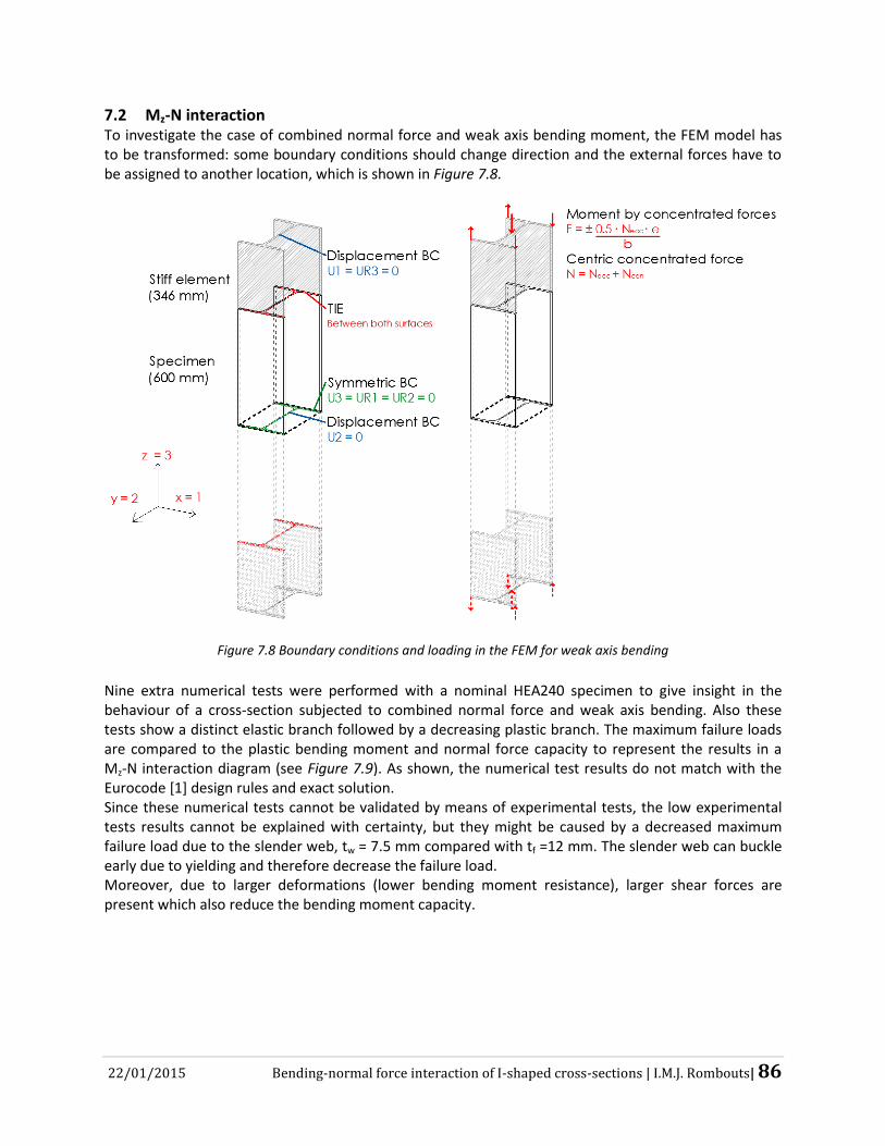
22/01/2015 Bending-normal force interaction of I-shaped cross-sections | I.M.J. Rombouts| 86
7.2 Mz-N interaction To investigate the case of combined normal force and weak axis bending moment, the FEM model has to be transformed: some boundary conditions should change direction and the external forces have to be assigned to another location, which is shown in Figure 7.8.
Figure 7.8 Boundary conditions and loading in the FEM for weak axis bending
Nine extra numerical tests were performed with a nominal HEA240 specimen to give insight in the behaviour of a cross-section subjected to combined normal force and weak axis bending. Also these tests show a distinct elastic branch followed by a decreasing plastic branch. The maximum failure loads are compared to the plastic bending moment and normal force capacity to represent the results in a Mz-N interaction diagram (see Figure 7.9). As shown, the numerical test results do not match with the Eurocode [1] design rules and exact solution. Since these numerical tests cannot be validated by means of experimental tests, the low experimental tests results cannot be explained with certainty, but they might be caused by a decreased maximum failure load due to the slender web, tw = 7.5 mm compared with tf =12 mm. The slender web can buckle early due to yielding and therefore decrease the failure load. Moreover, due to larger deformations (lower bending moment resistance), larger shear forces are present which also reduce the bending moment capacity.

22/01/2015 Bending-normal force interaction of I-shaped cross-sections | I.M.J. Rombouts| 87
Figure 7.9 Mz-N interaction of nominal HEA240 specimens
7.3 Tension as normal force While in most of the cases, MN-interaction is aimed at combined compression and bending moment, the Eurocode [1] M-N interaction design rules are valid for both compression and tension. Therefore one extra numerical test is performed with ratio n ≈ 0.4 and nominal HEA240 to investigate the difference in reduced bending moment capacity under tension and compression. For this investigation the nominal material model including strain hardening is used, as shown in paragraph 7.2. The force-deformation diagram of this numerical test is shown in Figure 7.10.
Figure 7.10 Force-deformation diagram of nominal HEA240 specimen under tension/compression
1
2
3
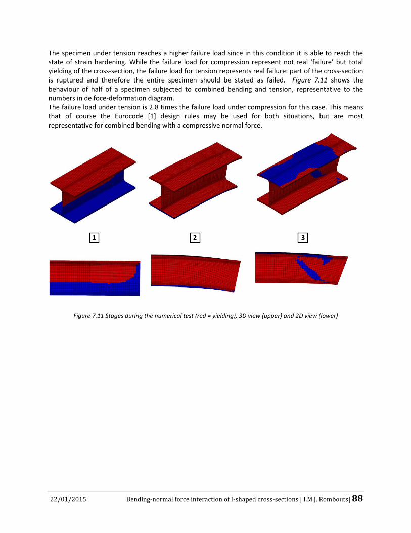
22/01/2015 Bending-normal force interaction of I-shaped cross-sections | I.M.J. Rombouts| 88
The specimen under tension reaches a higher failure load since in this condition it is able to reach the state of strain hardening. While the failure load for compression represent not real ‘failure’ but total yielding of the cross-section, the failure load for tension represents real failure: part of the cross-section is ruptured and therefore the entire specimen should be stated as failed. Figure 7.11 shows the behaviour of half of a specimen subjected to combined bending and tension, representative to the numbers in de foce-deformation diagram. The failure load under tension is 2.8 times the failure load under compression for this case. This means that of course the Eurocode [1] design rules may be used for both situations, but are most representative for combined bending with a compressive normal force.
Figure 7.11 Stages during the numerical test (red = yielding), 3D view (upper) and 2D view (lower)
1 2 3
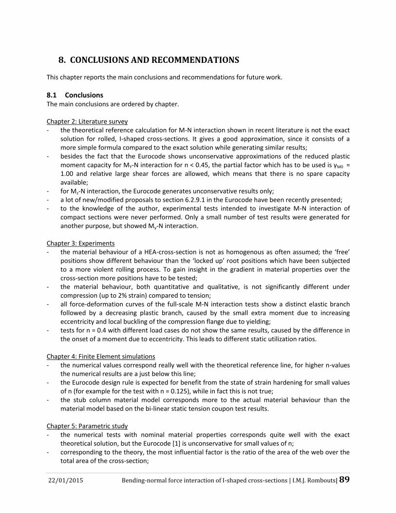
22/01/2015 Bending-normal force interaction of I-shaped cross-sections | I.M.J. Rombouts| 89
8. CONCLUSIONS AND RECOMMENDATIONS
This chapter reports the main conclusions and recommendations for future work.
8.1 Conclusions The main conclusions are ordered by chapter. Chapter 2: Literature survey - the theoretical reference calculation for M-N interaction shown in recent literature is not the exact
solution for rolled, I-shaped cross-sections. It gives a good approximation, since it consists of a more simple formula compared to the exact solution while generating similar results;
- besides the fact that the Eurocode shows unconservative approximations of the reduced plastic moment capacity for MY-N interaction for n < 0.45, the partial factor which has to be used is γM0 = 1.00 and relative large shear forces are allowed, which means that there is no spare capacity available;
- for Mz-N interaction, the Eurocode generates unconservative results only; - a lot of new/modified proposals to section 6.2.9.1 in the Eurocode have been recently presented; - to the knowledge of the author, experimental tests intended to investigate M-N interaction of
compact sections were never performed. Only a small number of test results were generated for another purpose, but showed My-N interaction.
Chapter 3: Experiments - the material behaviour of a HEA-cross-section is not as homogenous as often assumed; the ‘free’
positions show different behaviour than the ‘locked up’ root positions which have been subjected to a more violent rolling process. To gain insight in the gradient in material properties over the cross-section more positions have to be tested;
- the material behaviour, both quantitative and qualitative, is not significantly different under compression (up to 2% strain) compared to tension;
- all force-deformation curves of the full-scale M-N interaction tests show a distinct elastic branch followed by a decreasing plastic branch, caused by the small extra moment due to increasing eccentricity and local buckling of the compression flange due to yielding;
- tests for n = 0.4 with different load cases do not show the same results, caused by the difference in the onset of a moment due to eccentricity. This leads to different static utilization ratios.
Chapter 4: Finite Element simulations - the numerical values correspond really well with the theoretical reference line, for higher n-values
the numerical results are a just below this line; - the Eurocode design rule is expected for benefit from the state of strain hardening for small values
of n (for example for the test with n = 0.125), while in fact this is not true; - the stub column material model corresponds more to the actual material behaviour than the
material model based on the bi-linear static tension coupon test results. Chapter 5: Parametric study - the numerical tests with nominal material properties corresponds quite well with the exact
theoretical solution, but the Eurocode [1] is unconservative for small values of n; - corresponding to the theory, the most influential factor is the ratio of the area of the web over the
total area of the cross-section;

22/01/2015 Bending-normal force interaction of I-shaped cross-sections | I.M.J. Rombouts| 90
- the HEM400 numerical test results deviate from the exact solution caused by their large moment of eccentricity, which results from their larger deformation at the maximum failure load, due to the stocky flanges;
- since it is shown that there is a linear relation between the yield stress and the reduced bending moment capacity, all numerical tests performed with steel grade S235 have been rescaled to S355 and S460 test results.
Chapter 6: Statistical evaluation - the partial safety factor used in the Eurocode [1] design rules for My-N interaction is acceptable for
steel grades S235 and S355 and slightly too low for S460; - since a large portion of the statistical evaluation is influenced by the distribution of the variables
and these distributions are constantly subjected to changes, the partial safety factor can change over time. Fortunately it seems like the distribution of the yield stress will only be more favourable, mainly leading to a decrease of the partial safety factor.
Chapter 7: Brief additional research - cross-sections with slender flanges (HEA, IPE, HEB), are not able to reach the state of strain hardening
due to ‘local buckling’ caused by yielding while cross-sections with stocky flanges (HEM) are, generating higher resistances;
- for cross-sections with slender flanges, the resistances at low values of n will not be ‘saved’ by the state of strain hardening, while for cross-sections with stocky flanges, it will;
- the Eurocode [1] design rules may be used for both tension as compression as the normal force, but are most representative for combined bending with a compressive normal force.
Main conclusion
The behaviour of a cross-section with slender flanges subjected to combined strong axis bending and normal force is similar to the theoretical (exact) behaviour. The partial safety factor used in the Eurocode design rules for My-N interaction is statistically acceptable for these cross-sections with steel grades S235, S355 and S460.
8.2 Recommendations - apart from this research, the gradient in material properties over the cross-section is very interesting
to investigate. More positions could be tested to gain insight in the differences in material properties over the cross-sections. For example, the material behaviour in the interesting position of the outermost flange tip of a cross-section can be tested by means of a small-scale compression test;
- the influence of shear forces on the bending moment capacity should be investigated, since the Eurocode [1] design rule for M-N interaction allows a shear force as big as half of the plastic shear capacity;
- the additional research about the influence of strain hardening should be performed for more values of n, but especially for more cross-sections to investigate the influence of the slenderness of the flanges;
- also the brief investigation into weak axis bending should be extended and the numerical model should be validated by means of experimental tests. Moreover, the Eurocode generates unsafe results only compared to the exact solution and again the partial safety factor is 1.0;

22/01/2015 Bending-normal force interaction of I-shaped cross-sections | I.M.J. Rombouts| 91
- although it is statistically allowed to use the Eurocode [1] design rules with partial safety factor 1.0 for cross-sections HEA240, HEB200, IPE330 and HEM400, it is recommended to use another design rule which is more accurate for low values of n. Since the exact solution requires a lot of computational time, the theoretical reference calculation could be a good alternative (max deviation of exact solution is 0.23%, see Part A: Literature survey [27[). This design rule requires calculation of as much as parameters as the Eurocode [1]. However, it generates unconservative approximations of the bending resistance for higher values of n, as shown in chapter 5. Therefore, it is recommended to use a newly proposed design rule, shown in equation (8.1) to (8.3). This formula requires a little less computational time and shows more accurate results. It is again composed of two curves with the border between the flanges and the web (without roots): the first, quadratic curve is equal to the theoretical reference calculation and the second one is a simple linear relation.
My,Ed = Mpl,y,Rd - NEd
2
4 ∙ tw ∙ fy,Rd for NEd ≤ Npl,w,Rd = hw ∙ tw ∙ fy (8.1)
My,Ed = MT
Npl,Rd - Npl,w,Rd ∙ (Npl,Rd - NEd) for NEd > Npl,w,Rd (8.2)
With MT = Mpl,y,Rd - Npl,w,Rd
2
4 ∙ tw ∙ fy,Rd (8.3)
Figure 8.1 shows the representation of the design rules in the well-known My-N interaction diagram, with the green dotted line representing the numerical HEA240 tests. Figure 8.2 makes it clear: the newly proposed design rules show the most accurate results compared to the numerical tests.
Figure 8.1 Comparison of numerical tests with design
rules (HEA240 cross-section)
Figure 8.2 re / rt of design rules (HEA240 cross-section)
The exact solution for the IPE330 cross-section differs the most from the others, therefore the newly proposed design rule is also checked for this cross-section, as shown in Figure 8.3 and Figure 8.4. For this situation, the exact solution and therefore theoretical reference calculation
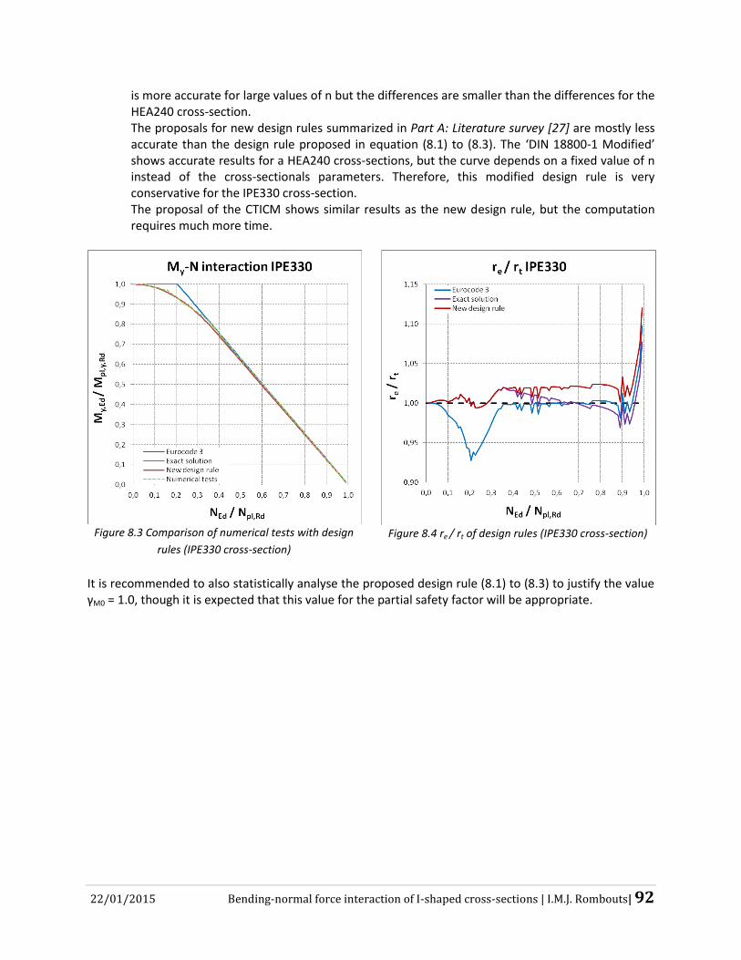
22/01/2015 Bending-normal force interaction of I-shaped cross-sections | I.M.J. Rombouts| 92
is more accurate for large values of n but the differences are smaller than the differences for the HEA240 cross-section. The proposals for new design rules summarized in Part A: Literature survey [27] are mostly less accurate than the design rule proposed in equation (8.1) to (8.3). The ‘DIN 18800-1 Modified’ shows accurate results for a HEA240 cross-sections, but the curve depends on a fixed value of n instead of the cross-sectionals parameters. Therefore, this modified design rule is very conservative for the IPE330 cross-section. The proposal of the CTICM shows similar results as the new design rule, but the computation requires much more time.
Figure 8.3 Comparison of numerical tests with design
rules (IPE330 cross-section)
Figure 8.4 re / rt of design rules (IPE330 cross-section)
It is recommended to also statistically analyse the proposed design rule (8.1) to (8.3) to justify the value γM0 = 1.0, though it is expected that this value for the partial safety factor will be appropriate.
22/01/2015 Bending-normal force interaction of I-shaped cross-sections | I.M.J. Rombouts| 93
9. REFERENCES
[1] Eurocode, 2011. EC 3: Design of steel structures- part 1-1: General rules and rules for buildings. Brussel: CEN
[2] Trahair NS, Bradford MA. The tandardi and design of steel structures to AS4100, 4rd ed. – Australian.
London: E & F Spon, 2007. [3] H.H. Snijder en H.M.G.M. Steenbergen, Krachtswerking. Grondslagen voor het berekenen en toetsen
van staalconstructies voor gebouwen volgens Eurocode 0, 1 en 3, Bouwen met Staal, Zoetermeer 2011, ISBN 978-90-72830-87-6.
[4] Perlynn, M.J. and Kulak, G.L., “Web slenderness limits for compact beams, Structural Engineering
Report No. 43,” University of Alberta, Department of Civil Engineering, Edmonton, 1973. [5] TGB Staalconstructies, NEN 6770, TGB 1990 – Staal constructies – Basiseisen en basisrekenregels voor
overwegend statisch belaste constructies, Delft: Nederlands Normalisatie Instituut, 1997. [6] Deutsches Institut für Normung, DIN 18800-1:2008-11. Steel structures – Part 1: Design and
construction, Berlin: Deutsches Institut für Normung, 2008. [7] Sedlacek, G., Spangemacher, R. and Hensen, W., 1989. Background documentation to Eurocode 3, The
b/t-ratios controlling the applicability of analysis models in Eurocode 3, Document 5.02. [8] Hasham, A.S. and Rasmussen, K.J.R., Interaction curves for locally buckled I-section beam columns,
Journal of Constructional Steel Research, 58, 2002. [9] Hasham, A.S. and Rasmussen, K.J.R., Nonlinear Analysis of Locally Buckled I-section Steel Beam-
Columns, Australian Journal of Structural Engineering, Vol.3 No 3, The University of Sydney, 2006. [10] Hasham, A.S. and Rasmussen, K.J.R., Interaction curves for locally buckled I-section beam columns,
Journal of Constructional Steel Research, 58, 2002. [11] Ziemian, R.D. ed., 2010. Guide to stability design criteria for metal structures. 6
th ed. Hoboken: John
Wiley & Sons, pp.993-1005.
[12] International Standards Office, 2009. ISO 6892-1 Metallic materials – Tensile testing. Geneva: ISO.
[13] ASTM, 2000, E9 – 09 Standard Test Methods of Compression Testing of Metallic Materials at Room Temperature.
[14] Spoorenberg, R.C., Snijder, H.H. & Hoenderkamp, J.C.D. (2012). Mechanical properties of roller bent wide flange sections – part 1: Experimental investigation. Journal of Constructional Steel Research, 68(1), 51-62.
[15] Rasmussen KJR, Burns T, Bezkorovainy P, and Bambach MR. Numerical modelling of stainless steel plates in compression. Journal of Constructional Steel Research 2003;59:1345-1362.
[16] Abaqus/CAE user’s manual, Dassault Systèmes, 2012.
22/01/2015 Bending-normal force interaction of I-shaped cross-sections | I.M.J. Rombouts| 94
[17] Johansson, B. et all., Commentary and worked examples to EN 1993-1-5-‘Plated structural elements’, JRC Scientific and Technical Rerpots, 2007.
[18] Simões da Silva, L., Rebelo C., Nethercot D. Marques, L., Simões, R., Vila Real, P.M.M. (2009), Statistical Evaluation of the Lateral-Torsional Buckling Resistance of Steel I-beams, Part 2: Variability of steel properties, J. of Const. Steel Res., 65, pp. 832-849.
[19] Braconi A. et all., OPUS – Optimising the seismic performance of steel and steel-concrete structures by tandardizing material quality control, Final report. Research Fund for Coal and Steel, Contract Agreement RFSR-CT-2007-00039, 2013.
[20] Alpsten, G., Variations in mechanical and cross-sectional properties of steel, State of the Art Report, Proceedings of the International Conference on the Planning and Design of Tall Buildings, ASCEIABSE,Lehigh University, August 1972.
[21] Taras A., ‘Contribution to the development of consistent stability design rules for steel members’, PhD Thesis, Technical University of Graz, Graz,Austria, 2010.
[22] Taras, A., Simões da Silva, L., European Recommendations for the Safety Assessment of Stability Design Rules for Steel Structures, University of Coimbra and Graz University of Technology, 1
st draft,
TC8-2012-06.
[23] CEN, European Committee for Standardization. EN 1990:2002, Basis of structural design, April 2002. Brussels.
[24] Simões da Silva, L., Tankova, T., Marques, L., Rebelo, C., Comparative Assessment of semi-probablistic methodologies for the safety assessment of stability design rules in the framework of annex D of EN 1990, University of Coimbra, March 2014.
[25] NEN-EN-10025, Hot rolled products of structural steels. Part 2, 3, 4 and 6, 2011.
[26] NEN-EN-10225 Weldable structural steels for fixed offshore structures - Technical delivery conditions.
[27] Rombouts, I.M.J., Bending-normal force interaction of I-shaped cross-sections, Part A: Literature Survey, University of Technology Eindhoven, August 2014.
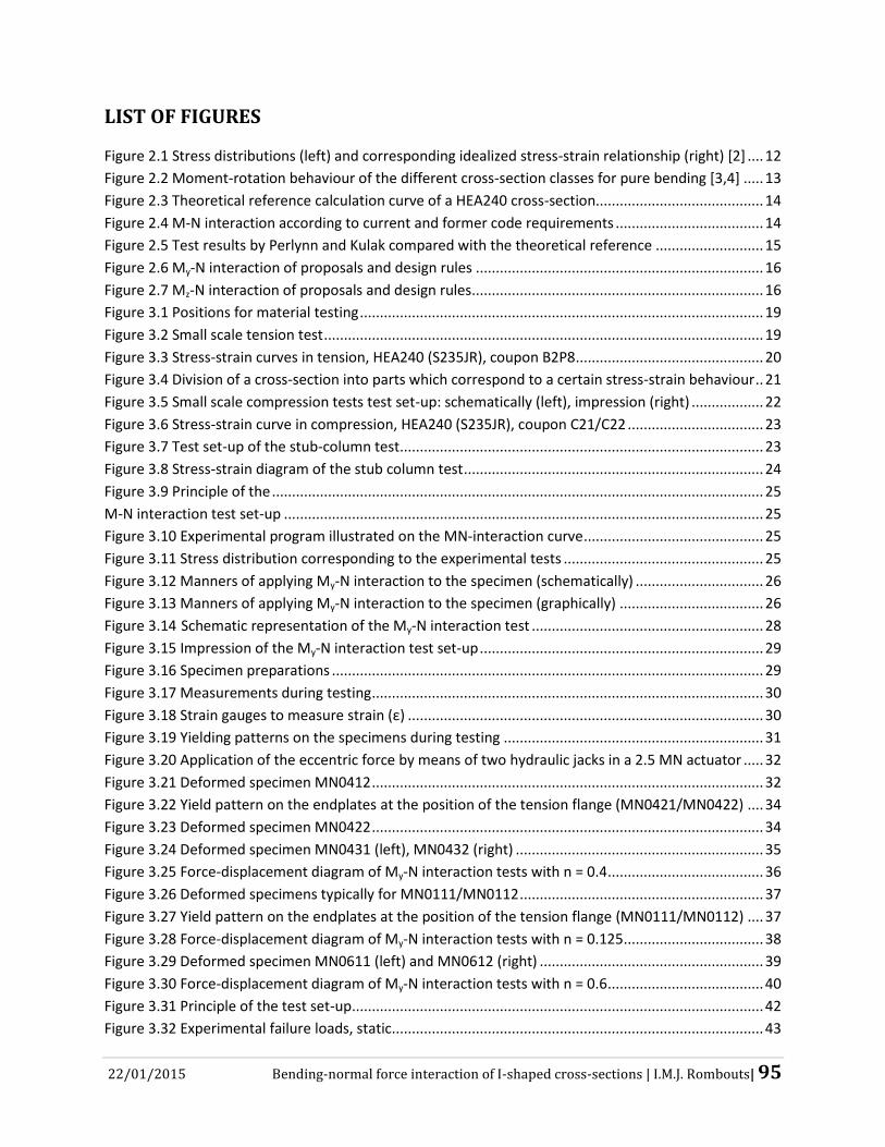
22/01/2015 Bending-normal force interaction of I-shaped cross-sections | I.M.J. Rombouts| 95
LIST OF FIGURES
Figure 2.1 Stress distributions (left) and corresponding idealized stress-strain relationship (right) [2] .... 12
Figure 2.2 Moment-rotation behaviour of the different cross-section classes for pure bending [3,4] ..... 13
Figure 2.3 Theoretical reference calculation curve of a HEA240 cross-section.......................................... 14
Figure 2.4 M-N interaction according to current and former code requirements ..................................... 14
Figure 2.5 Test results by Perlynn and Kulak compared with the theoretical reference ........................... 15
Figure 2.6 My-N interaction of proposals and design rules ........................................................................ 16
Figure 2.7 Mz-N interaction of proposals and design rules......................................................................... 16
Figure 3.1 Positions for material testing ..................................................................................................... 19
Figure 3.2 Small scale tension test .............................................................................................................. 19
Figure 3.3 Stress-strain curves in tension, HEA240 (S235JR), coupon B2P8 ............................................... 20
Figure 3.4 Division of a cross-section into parts which correspond to a certain stress-strain behaviour .. 21
Figure 3.5 Small scale compression tests test set-up: schematically (left), impression (right) .................. 22
Figure 3.6 Stress-strain curve in compression, HEA240 (S235JR), coupon C21/C22 .................................. 23
Figure 3.7 Test set-up of the stub-column test ........................................................................................... 23
Figure 3.8 Stress-strain diagram of the stub column test ........................................................................... 24
Figure 3.9 Principle of the ........................................................................................................................... 25
M-N interaction test set-up ........................................................................................................................ 25
Figure 3.10 Experimental program illustrated on the MN-interaction curve ............................................. 25
Figure 3.11 Stress distribution corresponding to the experimental tests .................................................. 25
Figure 3.12 Manners of applying My-N interaction to the specimen (schematically) ................................ 26
Figure 3.13 Manners of applying My-N interaction to the specimen (graphically) .................................... 26
Figure 3.14 Schematic representation of the My-N interaction test .......................................................... 28
Figure 3.15 Impression of the My-N interaction test set-up ....................................................................... 29
Figure 3.16 Specimen preparations ............................................................................................................ 29
Figure 3.17 Measurements during testing .................................................................................................. 30
Figure 3.18 Strain gauges to measure strain (ε) ......................................................................................... 30
Figure 3.19 Yielding patterns on the specimens during testing ................................................................. 31
Figure 3.20 Application of the eccentric force by means of two hydraulic jacks in a 2.5 MN actuator ..... 32
Figure 3.21 Deformed specimen MN0412 .................................................................................................. 32
Figure 3.22 Yield pattern on the endplates at the position of the tension flange (MN0421/MN0422) .... 34
Figure 3.23 Deformed specimen MN0422 .................................................................................................. 34
Figure 3.24 Deformed specimen MN0431 (left), MN0432 (right) .............................................................. 35
Figure 3.25 Force-displacement diagram of My-N interaction tests with n = 0.4 ....................................... 36
Figure 3.26 Deformed specimens typically for MN0111/MN0112 ............................................................. 37
Figure 3.27 Yield pattern on the endplates at the position of the tension flange (MN0111/MN0112) .... 37
Figure 3.28 Force-displacement diagram of My-N interaction tests with n = 0.125 ................................... 38
Figure 3.29 Deformed specimen MN0611 (left) and MN0612 (right) ........................................................ 39
Figure 3.30 Force-displacement diagram of My-N interaction tests with n = 0.6 ....................................... 40
Figure 3.31 Principle of the test set-up ....................................................................................................... 42
Figure 3.32 Experimental failure loads, static ............................................................................................. 43
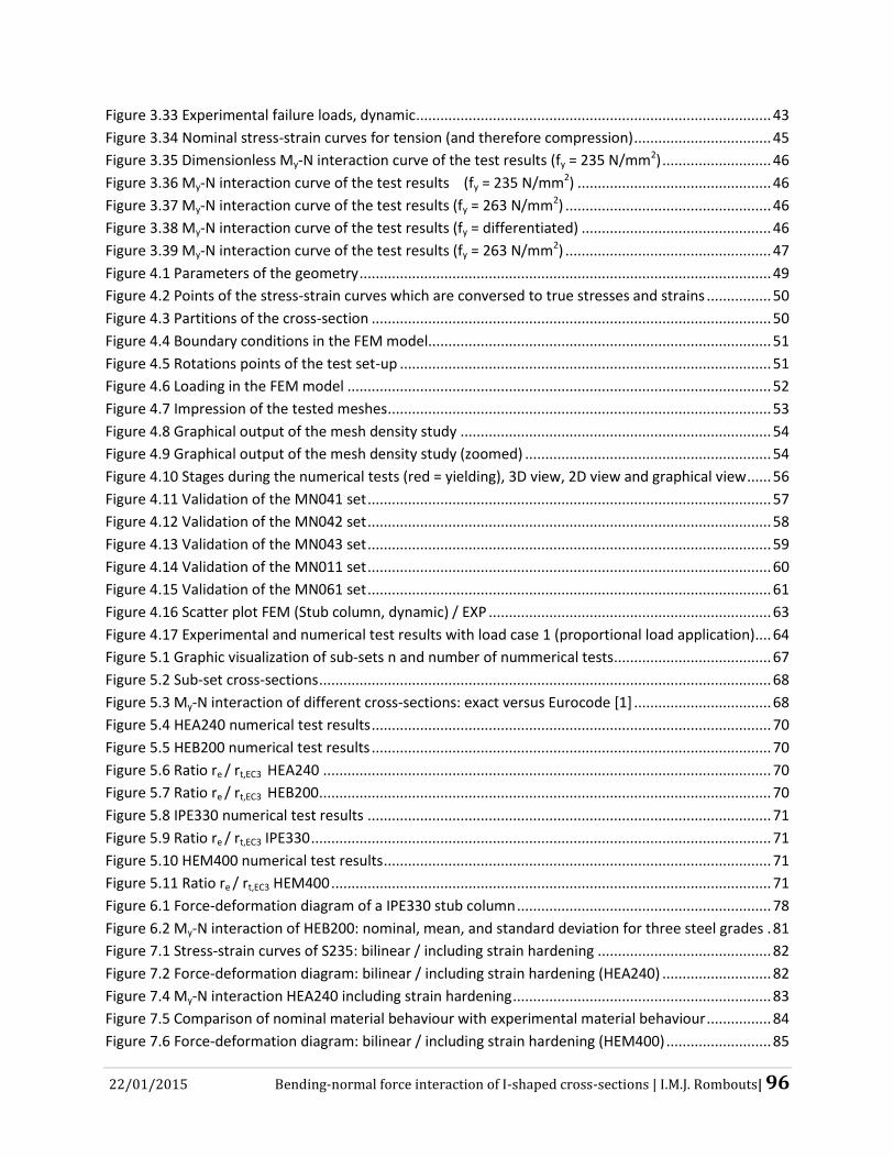
22/01/2015 Bending-normal force interaction of I-shaped cross-sections | I.M.J. Rombouts| 96
Figure 3.33 Experimental failure loads, dynamic ........................................................................................ 43
Figure 3.34 Nominal stress-strain curves for tension (and therefore compression) .................................. 45
Figure 3.35 Dimensionless My-N interaction curve of the test results (fy = 235 N/mm2) ........................... 46
Figure 3.36 My-N interaction curve of the test results (fy = 235 N/mm2) ................................................ 46
Figure 3.37 My-N interaction curve of the test results (fy = 263 N/mm2) ................................................... 46
Figure 3.38 My-N interaction curve of the test results (fy = differentiated) ............................................... 46
Figure 3.39 My-N interaction curve of the test results (fy = 263 N/mm2) ................................................... 47
Figure 4.1 Parameters of the geometry ...................................................................................................... 49
Figure 4.2 Points of the stress-strain curves which are conversed to true stresses and strains ................ 50
Figure 4.3 Partitions of the cross-section ................................................................................................... 50
Figure 4.4 Boundary conditions in the FEM model..................................................................................... 51
Figure 4.5 Rotations points of the test set-up ............................................................................................ 51
Figure 4.6 Loading in the FEM model ......................................................................................................... 52
Figure 4.7 Impression of the tested meshes ............................................................................................... 53
Figure 4.8 Graphical output of the mesh density study ............................................................................. 54
Figure 4.9 Graphical output of the mesh density study (zoomed) ............................................................. 54
Figure 4.10 Stages during the numerical tests (red = yielding), 3D view, 2D view and graphical view ...... 56
Figure 4.11 Validation of the MN041 set .................................................................................................... 57
Figure 4.12 Validation of the MN042 set .................................................................................................... 58
Figure 4.13 Validation of the MN043 set .................................................................................................... 59
Figure 4.14 Validation of the MN011 set .................................................................................................... 60
Figure 4.15 Validation of the MN061 set .................................................................................................... 61
Figure 4.16 Scatter plot FEM (Stub column, dynamic) / EXP ...................................................................... 63
Figure 4.17 Experimental and numerical test results with load case 1 (proportional load application).... 64
Figure 5.1 Graphic visualization of sub-sets n and number of nummerical tests ....................................... 67
Figure 5.2 Sub-set cross-sections ................................................................................................................ 68
Figure 5.3 My-N interaction of different cross-sections: exact versus Eurocode [1] .................................. 68
Figure 5.4 HEA240 numerical test results ................................................................................................... 70
Figure 5.5 HEB200 numerical test results ................................................................................................... 70
Figure 5.6 Ratio re / rt,EC3 HEA240 ............................................................................................................... 70
Figure 5.7 Ratio re / rt,EC3 HEB200 ................................................................................................................ 70
Figure 5.8 IPE330 numerical test results .................................................................................................... 71
Figure 5.9 Ratio re / rt,EC3 IPE330 .................................................................................................................. 71
Figure 5.10 HEM400 numerical test results ................................................................................................ 71
Figure 5.11 Ratio re / rt,EC3 HEM400 ............................................................................................................. 71
Figure 6.1 Force-deformation diagram of a IPE330 stub column ............................................................... 78
Figure 6.2 My-N interaction of HEB200: nominal, mean, and standard deviation for three steel grades . 81
Figure 7.1 Stress-strain curves of S235: bilinear / including strain hardening ........................................... 82
Figure 7.2 Force-deformation diagram: bilinear / including strain hardening (HEA240) ........................... 82
Figure 7.4 My-N interaction HEA240 including strain hardening ................................................................ 83
Figure 7.5 Comparison of nominal material behaviour with experimental material behaviour ................ 84
Figure 7.6 Force-deformation diagram: bilinear / including strain hardening (HEM400) .......................... 85

22/01/2015 Bending-normal force interaction of I-shaped cross-sections | I.M.J. Rombouts| 97
Figure 7.7 My-N interaction HEM400 including strain hardening ............................................................... 85
Figure 7.8 Boundary conditions and loading in the FEM for weak axis bending ........................................ 86
Figure 7.9 Mz-N interaction of nominal HEA240 specimens ....................................................................... 87
Figure 7.10 Force-deformation diagram of nominal HEA240 specimen under tension/compression ....... 87
Figure 7.11 Stages during the numerical test (red = yielding), 3D view (upper) and 2D view (lower) ....... 88
Figure 8.1 Comparison of numerical tests with design rules (HEA240 cross-section)................................ 91
Figure 8.2 re / rt of design rules (HEA240 cross-section) ............................................................................. 91
Figure 8.3 Comparison of numerical tests with design rules (IPE330 cross-section) ................................. 92
Figure 8.4 re / rt of design rules (IPE330 cross-section) ............................................................................... 92
LIST OF TABLES
Table 3.1 Measured dynamic and static yield stresses in tension .............................................................. 20
Table 3.2 Measured dynamic and calculated static yield stresses in compression .................................... 22
Table 3.3 Description and theoretical failure load of the specimens ......................................................... 27
Table 3.4 My-N interaction experimental test results with n = 0.4............................................................. 37
Table 3.5 My-N interaction experimental test results with n = 0.125 ........................................................ 39
Table 3.6 My-N interaction experimental test results with n = 0.6............................................................. 40
Table 3.7 Tension and compression yield stresses ..................................................................................... 41
Table 3.8 All My-N interaction experimental test results........................................................................... 43
Table 4.1 Results of the mesh density study on n = 0.4 (material properties: SC, dynamic) ..................... 53
Table 4.2 Overview of the difference between experiments and FE simulations, n = 0.4 (MN041) .......... 57
Table 4.3 Overview of the difference between experiments and FE simulations, n = 0.4 (MN042) .......... 58
Table 4.4 Overview of the difference between experiments and FE simulations, n = 0.4 (MN043) .......... 59
Table 4.5 Overview of the difference between experiments and FE simulations, n = 0.125 (MN01) ........ 60
Table 4.6 Overview of the difference between experiments and FE simulations, n = 0.6 (MN06) ............ 61
Table 4.7 Overview of the difference between experiments and FE simulations ...................................... 63
Table 5.1 Adopted reference yield stress distributions [18, 19] ................................................................. 66
Table 5.2 Adopted geometrical distributions [20, 21] ................................................................................ 66
Table 5.3 Cross-sections with their parameters relative to a HEA240 cross-section ................................. 67
Table 5.4 Numerical test results of the investigation on the influence of the yield stress (steel grade) ... 69
Table 6.1 Stepwise methodology to determine partial safety factor [23] ................................................. 74
Table 6.2 Statistical results of numerical tests ........................................................................................... 75
Table 6.3 Adopted reference yield stress distributions [18, 19] ................................................................ 76
Table 6.4 Cross-sectional classification ....................................................................................................... 77
Table 6.5 Stepwise methodology to determine partial safety factor [23] ................................................. 79
Table 6.6 Partial safety factors for higher steel grades per cross-section .................................................. 80
Table 7.1 Numerical test results: with and without strain hardeningHEA240 .......................................... 83

22/01/2015 Bending-normal force interaction of I-shaped cross-sections | I.M.J. Rombouts| 98
10. ANNEXES
10.1 Positions of the tensile coupons

22/01/2015 Bending-normal force interaction of I-shaped cross-sections | I.M.J. Rombouts| 99
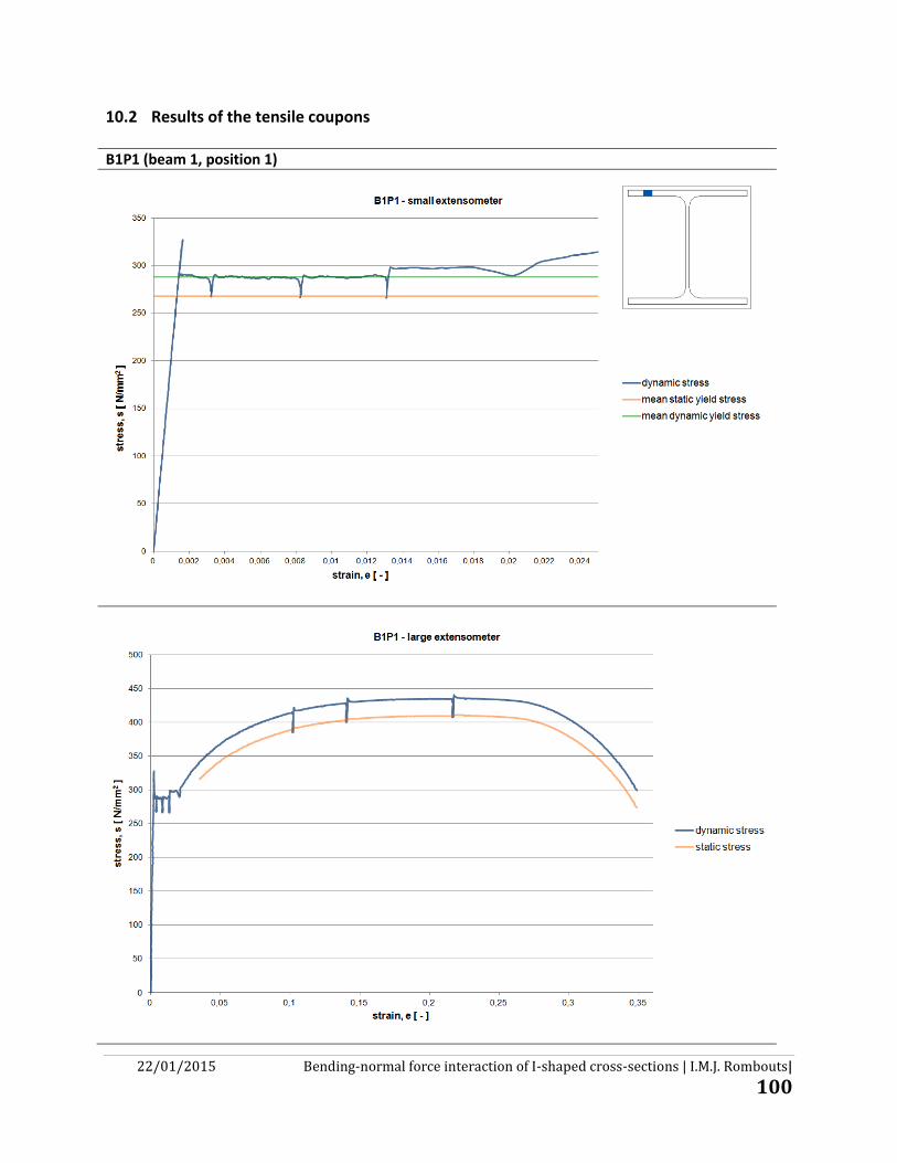
22/01/2015 Bending-normal force interaction of I-shaped cross-sections | I.M.J. Rombouts|
100
10.2 Results of the tensile coupons B1P1 (beam 1, position 1)

22/01/2015 Bending-normal force interaction of I-shaped cross-sections | I.M.J. Rombouts|
101
B1P2 (beam 1, position 2)

22/01/2015 Bending-normal force interaction of I-shaped cross-sections | I.M.J. Rombouts|
102
B1P8 (beam 1, position 8)

22/01/2015 Bending-normal force interaction of I-shaped cross-sections | I.M.J. Rombouts|
103
B1P9 (beam 1, position 9)
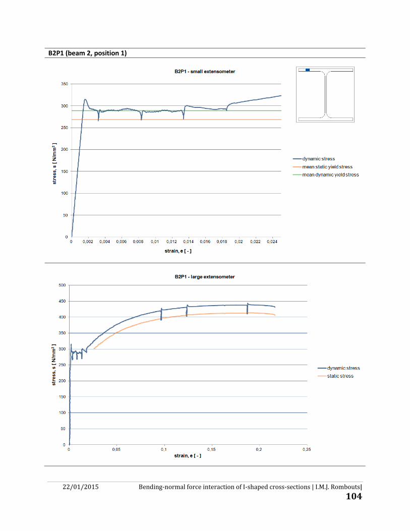
22/01/2015 Bending-normal force interaction of I-shaped cross-sections | I.M.J. Rombouts|
104
B2P1 (beam 2, position 1)

22/01/2015 Bending-normal force interaction of I-shaped cross-sections | I.M.J. Rombouts|
105
B2P2 (beam 2, position 2)
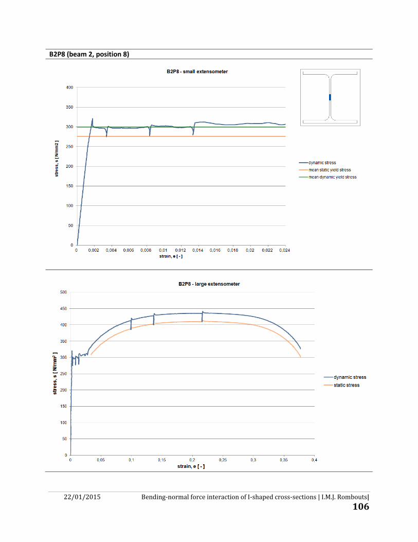
22/01/2015 Bending-normal force interaction of I-shaped cross-sections | I.M.J. Rombouts|
106
B2P8 (beam 2, position 8)

22/01/2015 Bending-normal force interaction of I-shaped cross-sections | I.M.J. Rombouts|
107
B2P9 (beam 2, position 7)

22/01/2015 Bending-normal force interaction of I-shaped cross-sections | I.M.J. Rombouts|
108
B4P1 (beam 4, position 1)
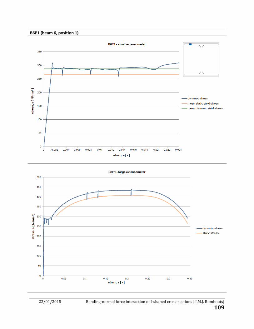
22/01/2015 Bending-normal force interaction of I-shaped cross-sections | I.M.J. Rombouts|
109
B6P1 (beam 6, position 1)
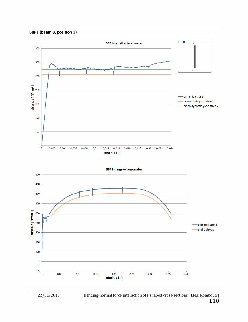
22/01/2015 Bending-normal force interaction of I-shaped cross-sections | I.M.J. Rombouts|
110
B8P1 (beam 8, position 1)
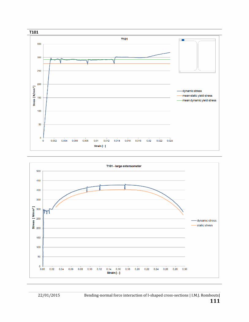
22/01/2015 Bending-normal force interaction of I-shaped cross-sections | I.M.J. Rombouts|
111
T101
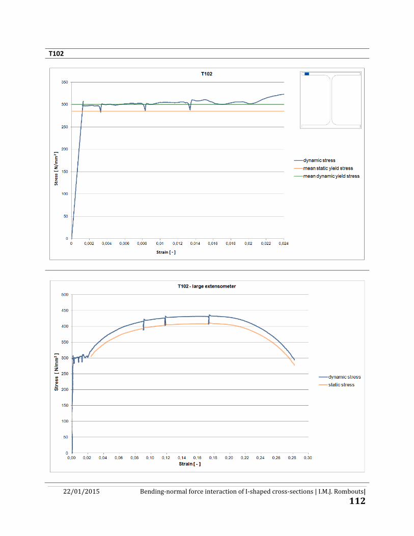
22/01/2015 Bending-normal force interaction of I-shaped cross-sections | I.M.J. Rombouts|
112
T102

22/01/2015 Bending-normal force interaction of I-shaped cross-sections | I.M.J. Rombouts|
113
T141
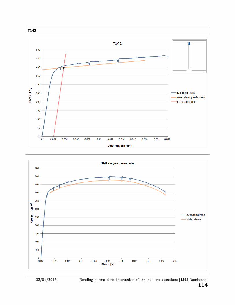
22/01/2015 Bending-normal force interaction of I-shaped cross-sections | I.M.J. Rombouts|
114
T142
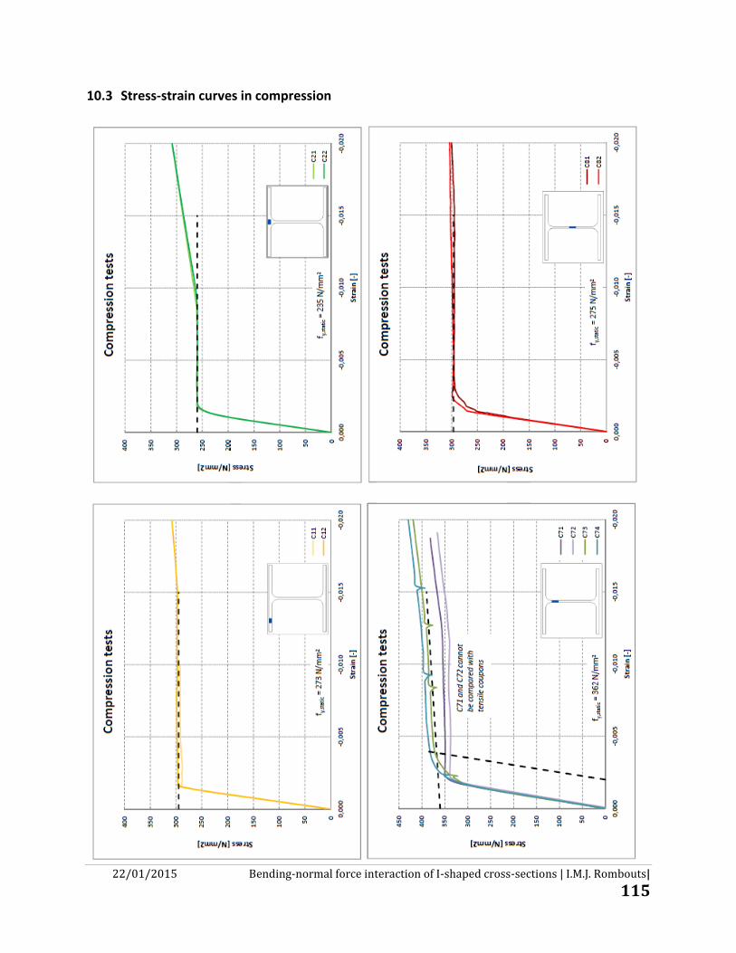
22/01/2015 Bending-normal force interaction of I-shaped cross-sections | I.M.J. Rombouts|
115
10.3 Stress-strain curves in compression
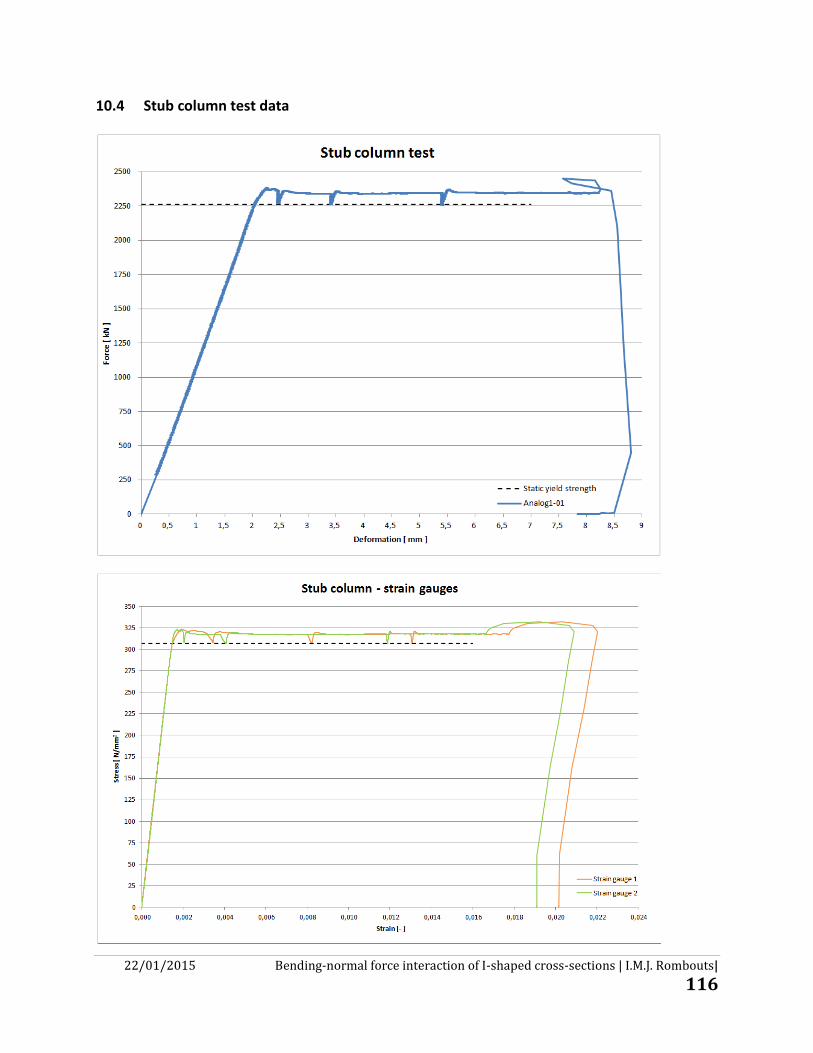
22/01/2015 Bending-normal force interaction of I-shaped cross-sections | I.M.J. Rombouts|
116
10.4 Stub column test data
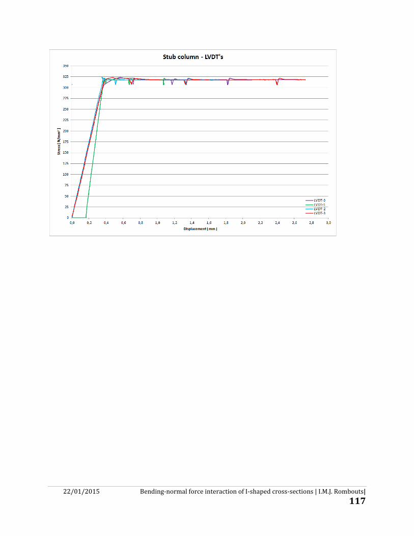
22/01/2015 Bending-normal force interaction of I-shaped cross-sections | I.M.J. Rombouts|
117

22/01/2015 Bending-normal force interaction of I-shaped cross-sections | I.M.J. Rombouts|
118
10.5 Stress-strain curves in compression and tension
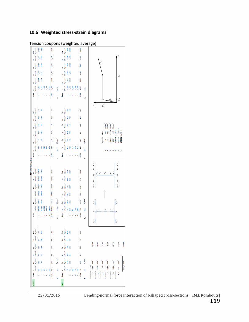
22/01/2015 Bending-normal force interaction of I-shaped cross-sections | I.M.J. Rombouts|
119
10.6 Weighted stress-strain diagrams Tension coupons (weighted average)

22/01/2015 Bending-normal force interaction of I-shaped cross-sections | I.M.J. Rombouts|
120
Compression coupons (weighted average)
Stub column (global)

22/01/2015 Bending-normal force interaction of I-shaped cross-sections | I.M.J. Rombouts|
121
10.7 Actual dimensions of the specimens
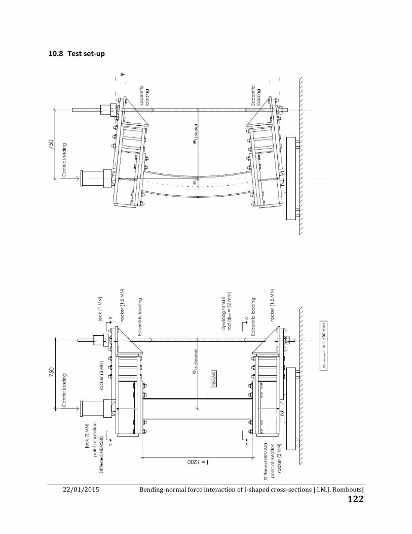
22/01/2015 Bending-normal force interaction of I-shaped cross-sections | I.M.J. Rombouts|
122
10.8 Test set-up

22/01/2015 Bending-normal force interaction of I-shaped cross-sections | I.M.J. Rombouts|
123

22/01/2015 Bending-normal force interaction of I-shaped cross-sections | I.M.J. Rombouts|
124
10.9 Test results MN0411
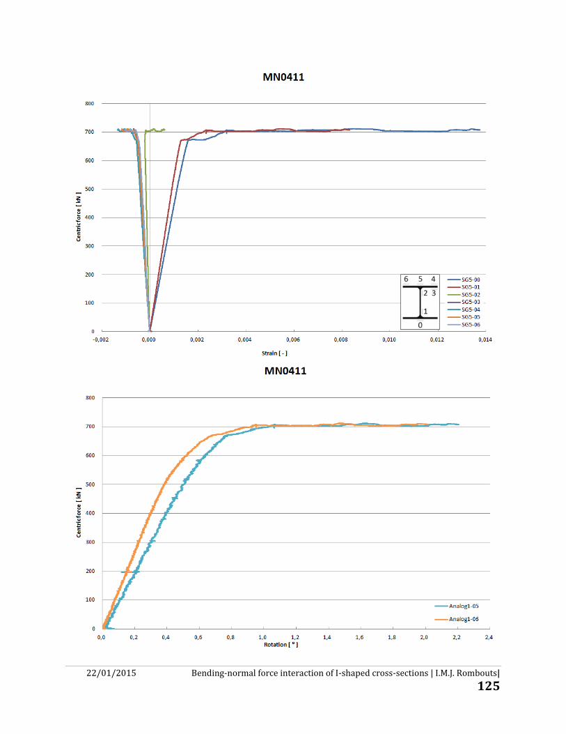
22/01/2015 Bending-normal force interaction of I-shaped cross-sections | I.M.J. Rombouts|
125

22/01/2015 Bending-normal force interaction of I-shaped cross-sections | I.M.J. Rombouts|
126
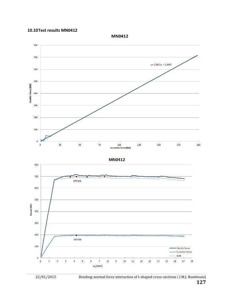
22/01/2015 Bending-normal force interaction of I-shaped cross-sections | I.M.J. Rombouts|
127
10.10 Test results MN0412

22/01/2015 Bending-normal force interaction of I-shaped cross-sections | I.M.J. Rombouts|
128
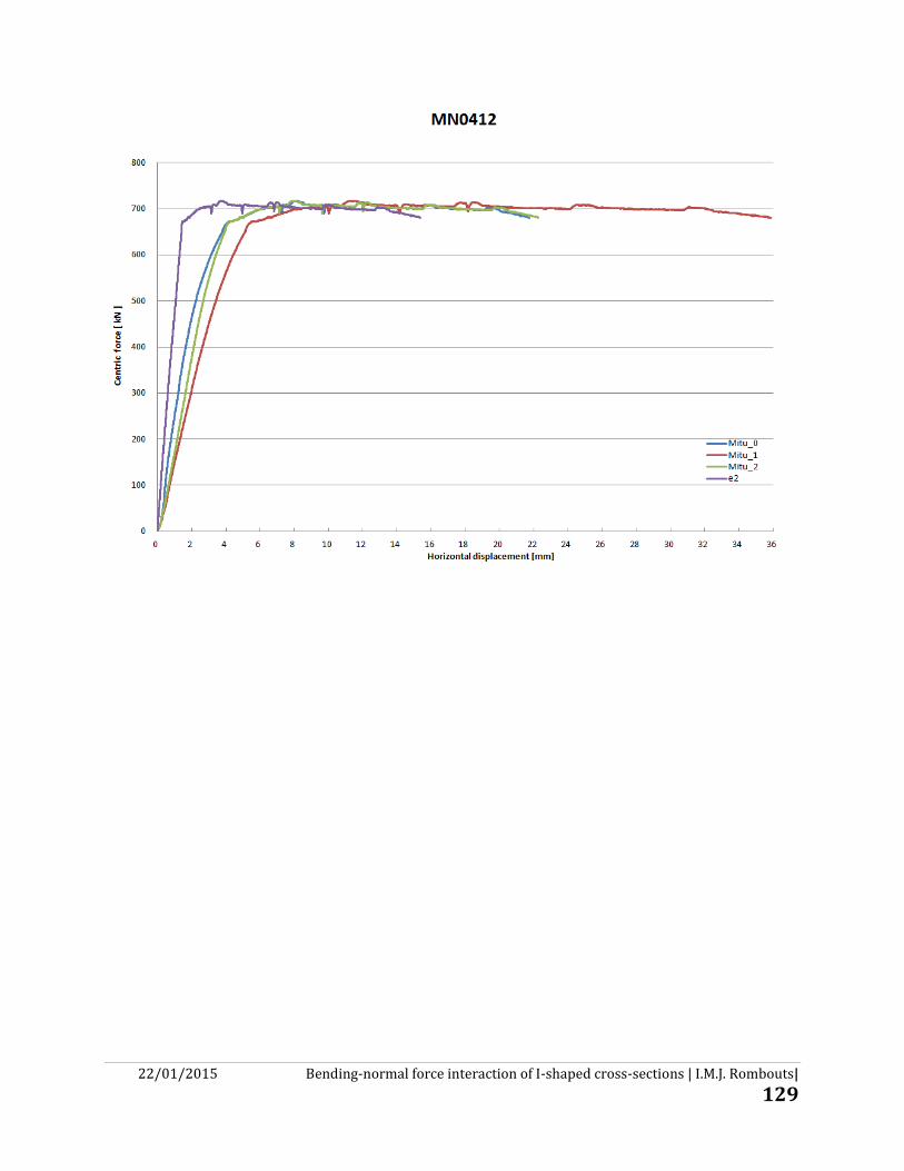
22/01/2015 Bending-normal force interaction of I-shaped cross-sections | I.M.J. Rombouts|
129
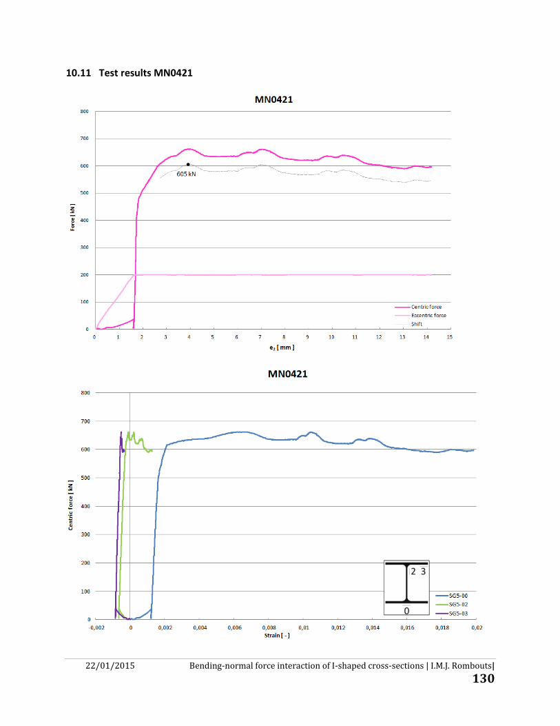
22/01/2015 Bending-normal force interaction of I-shaped cross-sections | I.M.J. Rombouts|
130
10.11 Test results MN0421

22/01/2015 Bending-normal force interaction of I-shaped cross-sections | I.M.J. Rombouts|
131

22/01/2015 Bending-normal force interaction of I-shaped cross-sections | I.M.J. Rombouts|
132
10.12 Test results MN0422

22/01/2015 Bending-normal force interaction of I-shaped cross-sections | I.M.J. Rombouts|
133
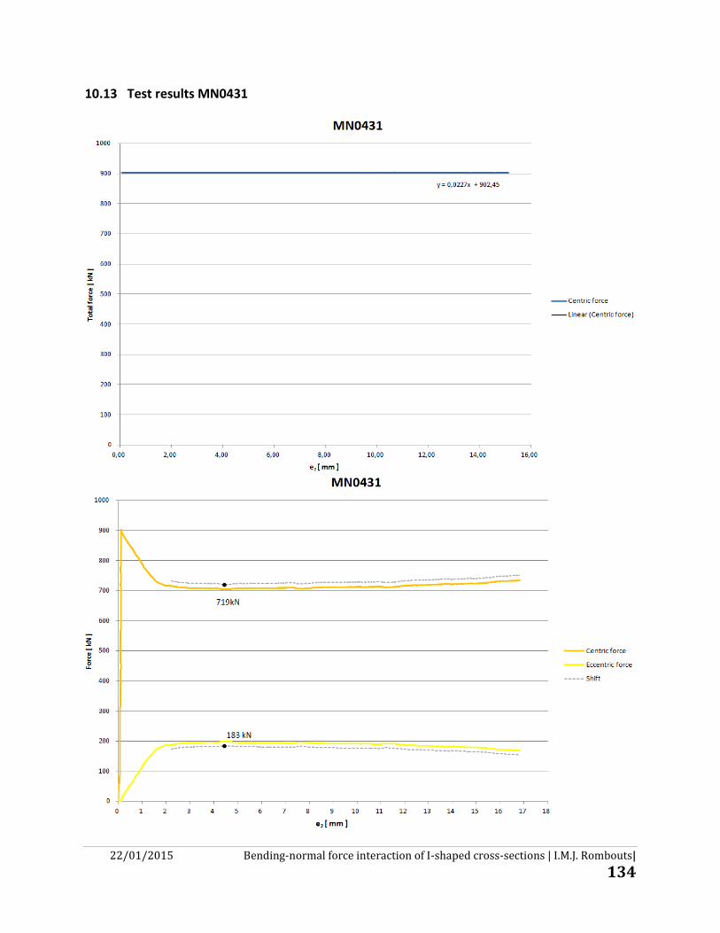
22/01/2015 Bending-normal force interaction of I-shaped cross-sections | I.M.J. Rombouts|
134
10.13 Test results MN0431

22/01/2015 Bending-normal force interaction of I-shaped cross-sections | I.M.J. Rombouts|
135
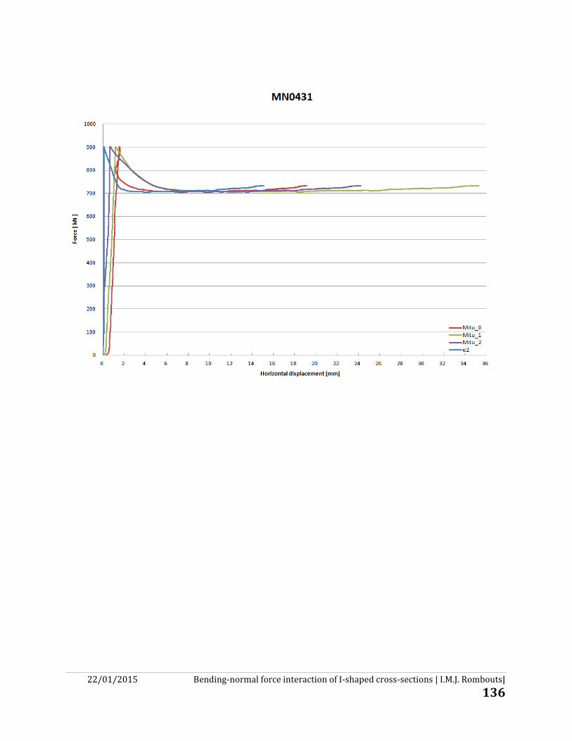
22/01/2015 Bending-normal force interaction of I-shaped cross-sections | I.M.J. Rombouts|
136

22/01/2015 Bending-normal force interaction of I-shaped cross-sections | I.M.J. Rombouts|
137
10.14 Test results MN0432

22/01/2015 Bending-normal force interaction of I-shaped cross-sections | I.M.J. Rombouts|
138

22/01/2015 Bending-normal force interaction of I-shaped cross-sections | I.M.J. Rombouts|
139
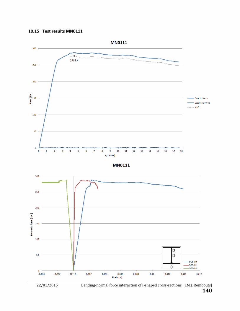
22/01/2015 Bending-normal force interaction of I-shaped cross-sections | I.M.J. Rombouts|
140
10.15 Test results MN0111
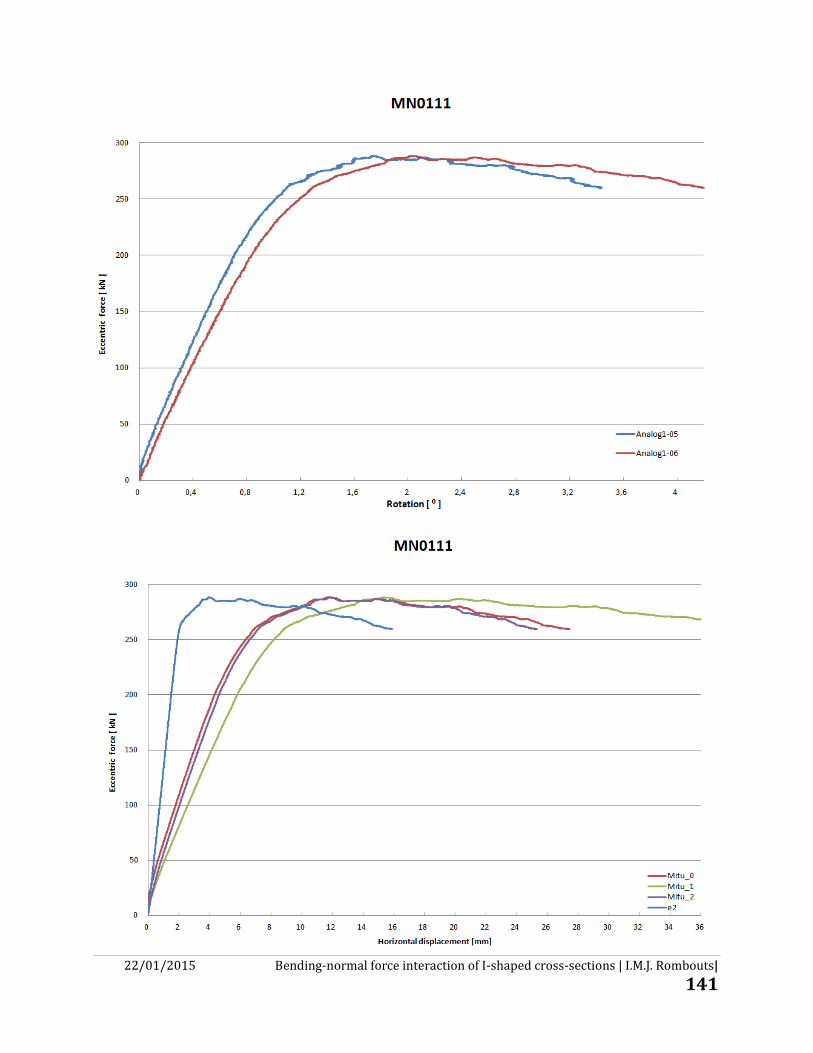
22/01/2015 Bending-normal force interaction of I-shaped cross-sections | I.M.J. Rombouts|
141
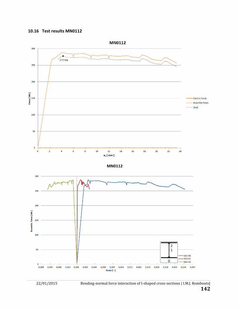
22/01/2015 Bending-normal force interaction of I-shaped cross-sections | I.M.J. Rombouts|
142
10.16 Test results MN0112
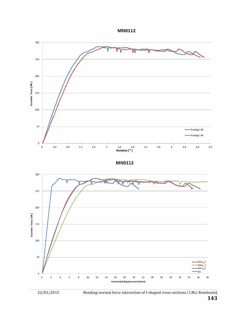
22/01/2015 Bending-normal force interaction of I-shaped cross-sections | I.M.J. Rombouts|
143
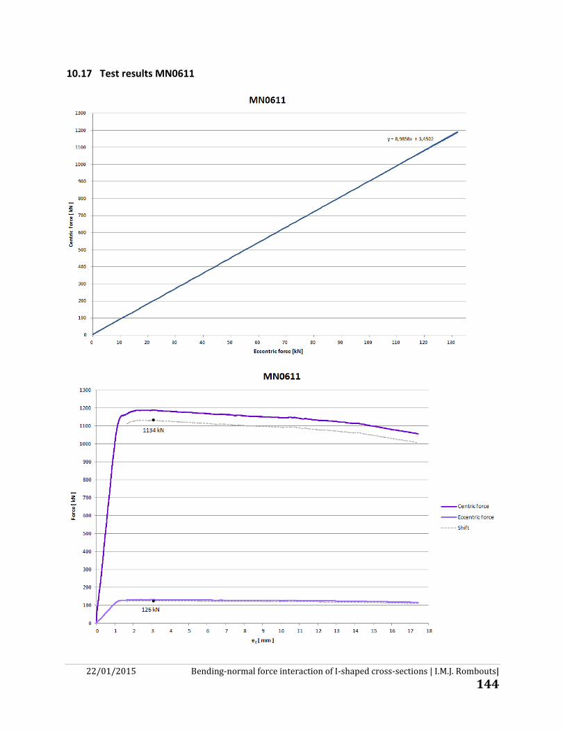
22/01/2015 Bending-normal force interaction of I-shaped cross-sections | I.M.J. Rombouts|
144
10.17 Test results MN0611

22/01/2015 Bending-normal force interaction of I-shaped cross-sections | I.M.J. Rombouts|
145
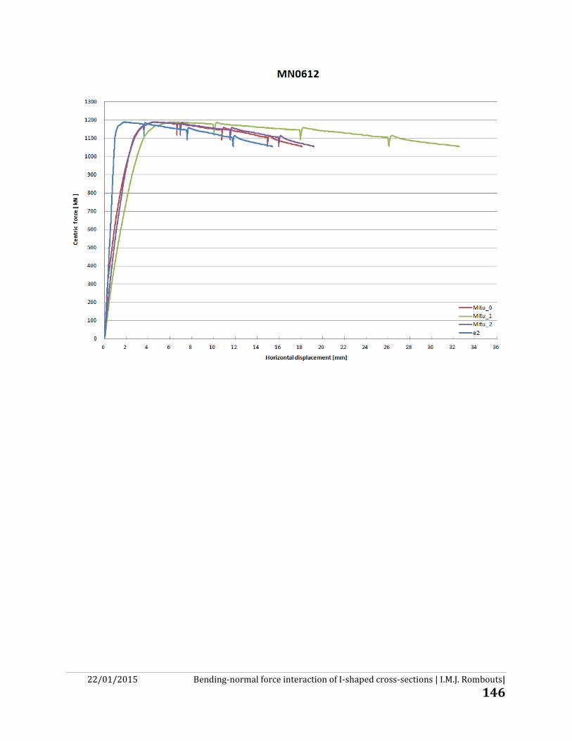
22/01/2015 Bending-normal force interaction of I-shaped cross-sections | I.M.J. Rombouts|
146
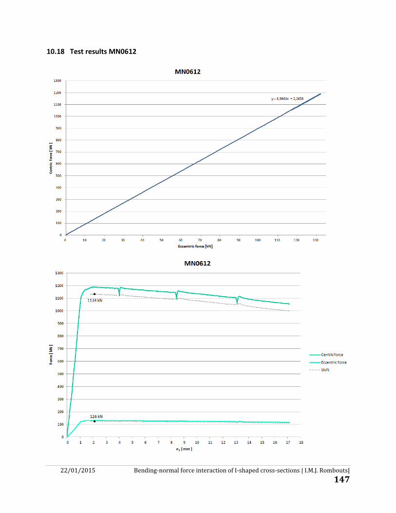
22/01/2015 Bending-normal force interaction of I-shaped cross-sections | I.M.J. Rombouts|
147
10.18 Test results MN0612
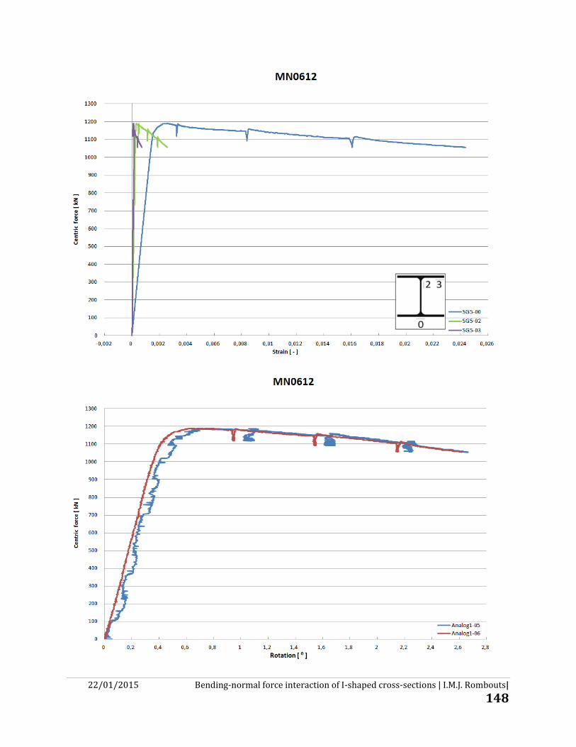
22/01/2015 Bending-normal force interaction of I-shaped cross-sections | I.M.J. Rombouts|
148

22/01/2015 Bending-normal force interaction of I-shaped cross-sections | I.M.J. Rombouts|
149

22/01/2015 Bending-normal force interaction of I-shaped cross-sections | I.M.J. Rombouts|
150
10.19 FEM model Python script
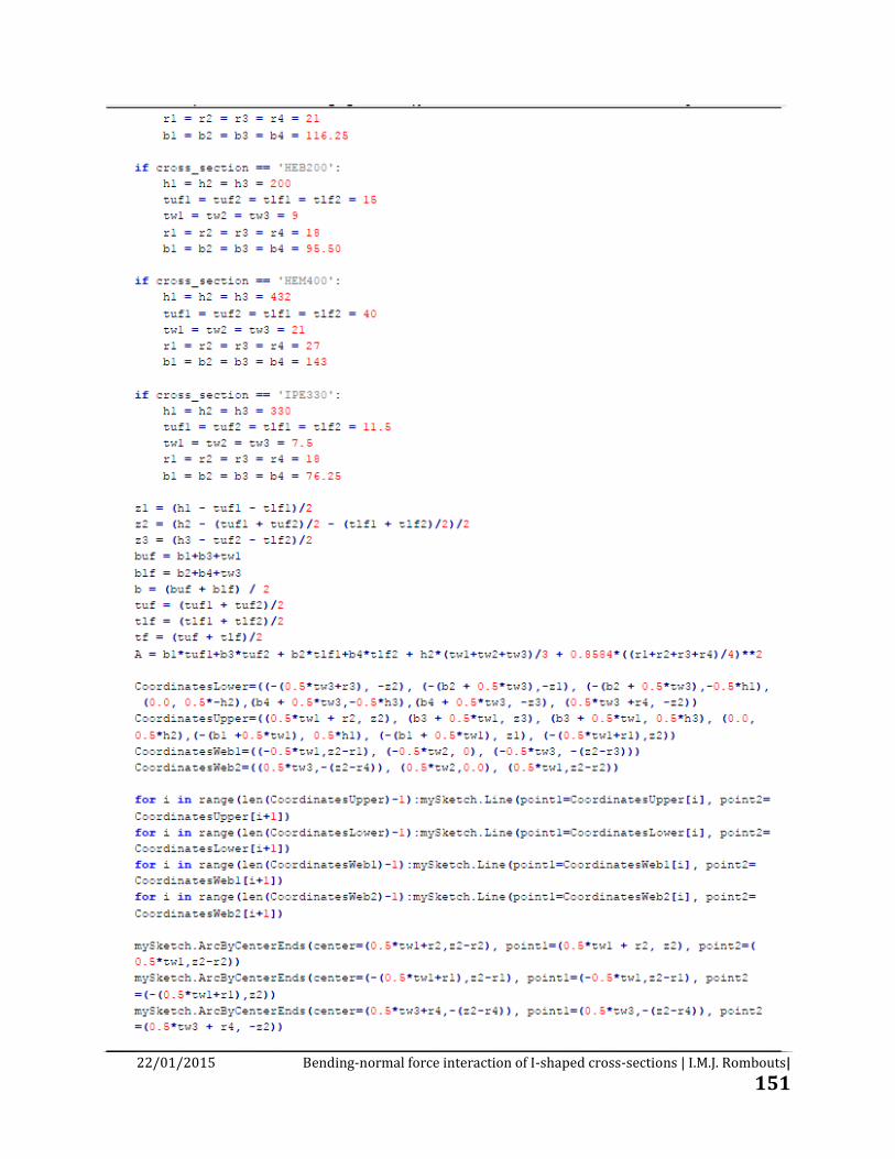
22/01/2015 Bending-normal force interaction of I-shaped cross-sections | I.M.J. Rombouts|
151

22/01/2015 Bending-normal force interaction of I-shaped cross-sections | I.M.J. Rombouts|
152

22/01/2015 Bending-normal force interaction of I-shaped cross-sections | I.M.J. Rombouts|
153
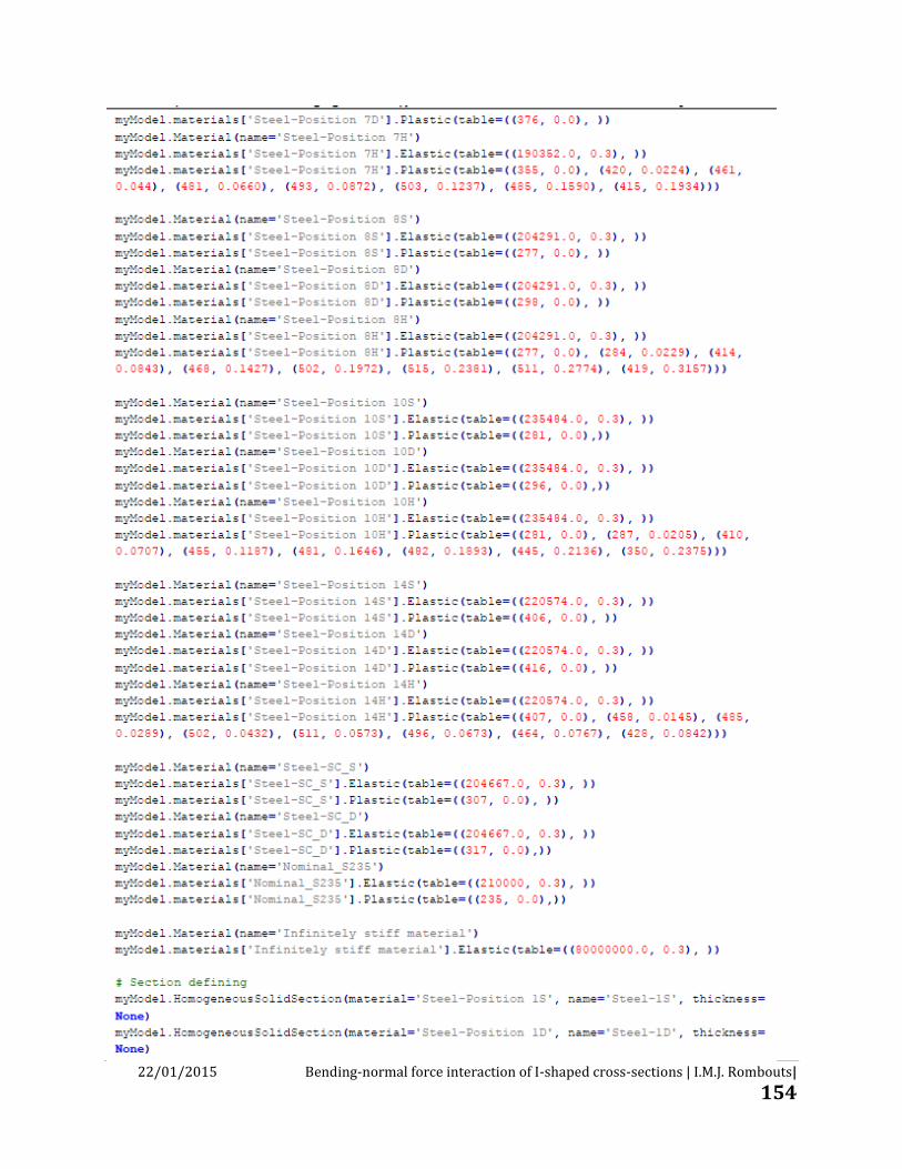
22/01/2015 Bending-normal force interaction of I-shaped cross-sections | I.M.J. Rombouts|
154

22/01/2015 Bending-normal force interaction of I-shaped cross-sections | I.M.J. Rombouts|
155

22/01/2015 Bending-normal force interaction of I-shaped cross-sections | I.M.J. Rombouts|
156

22/01/2015 Bending-normal force interaction of I-shaped cross-sections | I.M.J. Rombouts|
157
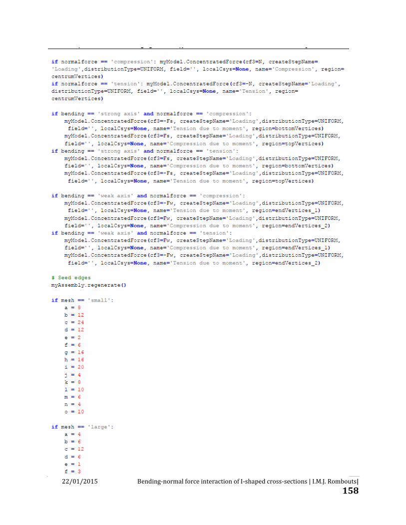
22/01/2015 Bending-normal force interaction of I-shaped cross-sections | I.M.J. Rombouts|
158
22/01/2015 Bending-normal force interaction of I-shaped cross-sections | I.M.J. Rombouts|
159
22/01/2015 Bending-normal force interaction of I-shaped cross-sections | I.M.J. Rombouts|
160

22/01/2015 Bending-normal force interaction of I-shaped cross-sections | I.M.J. Rombouts|
161

22/01/2015 Bending-normal force interaction of I-shaped cross-sections | I.M.J. Rombouts|
162

22/01/2015 Bending-normal force interaction of I-shaped cross-sections | I.M.J. Rombouts|
163
10.20 Strain gauge validation
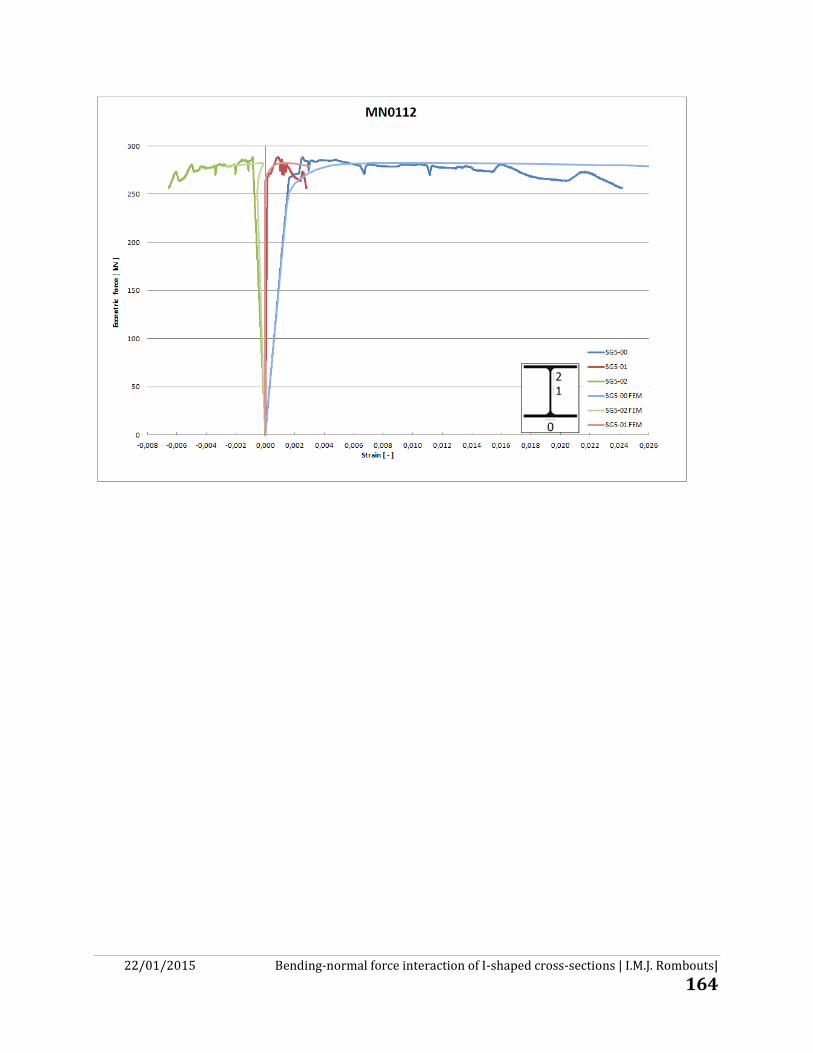
22/01/2015 Bending-normal force interaction of I-shaped cross-sections | I.M.J. Rombouts|
164

22/01/2015 Bending-normal force interaction of I-shaped cross-sections | I.M.J. Rombouts|
165
10.21 Flow chart for the determination of Vrt
22/01/2015 Bending-normal force interaction of I-shaped cross-sections | I.M.J. Rombouts|
166
10.22 Statistical evaluation

0.00 < n < 0.25 25 tests
0.25 ≤ n < 0.50 27 tests
0.50 ≤ n < 0.75 25 tests
0.75 ≤ n < 1.00 22 tests
Total 99 tests
b 0,981
Δbar ‐0,004
sΔ2
0,0002
Vδ 0,0128
γM* 0,993
TEST RESULTS
M y ‐N INTERACTION DIAGRAM
HEA240
0,8
0,9
1,0
My‐N interaction HEA240
1
0,0
0,1
0,2
0,3
0,4
0,5
0,6
0,7
0,8
0,0 0,1 0,2 0,3 0,4 0,5 0,6 0,7 0,8 0,9 1,0
My,Ed
/ M
pl,y,Rd
NEd / Npl,Rd
Nummerical testsEurocode 3 nominal HEA240Exact solution nominal HEA240
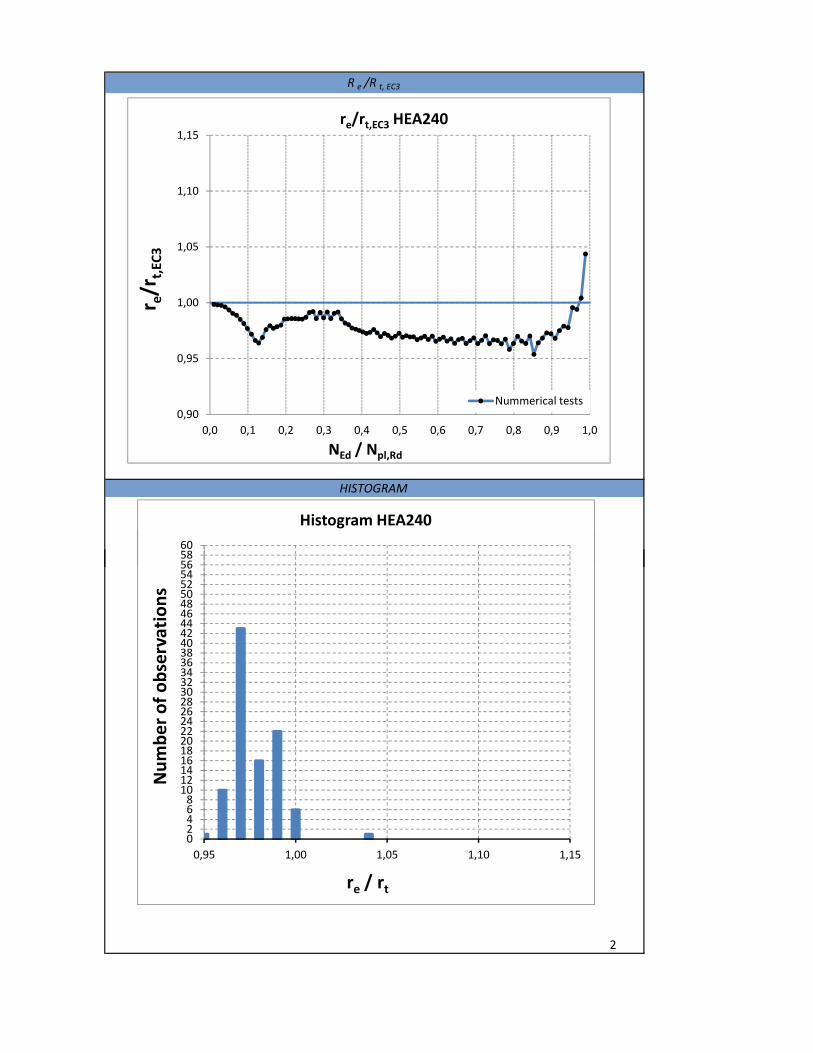
R e /R t, EC3
HISTOGRAM
565860
Histogram HEA240
0,90
0,95
1,00
1,05
1,10
1,15
0,0 0,1 0,2 0,3 0,4 0,5 0,6 0,7 0,8 0,9 1,0
r e/r
t,EC3
NEd / Npl,Rd
re/rt,EC3 HEA240
Nummerical tests
2
024681012141618202224262830323436384042444648505254565860
0,95 1,00 1,05 1,10 1,15
Number of observations
re / rt
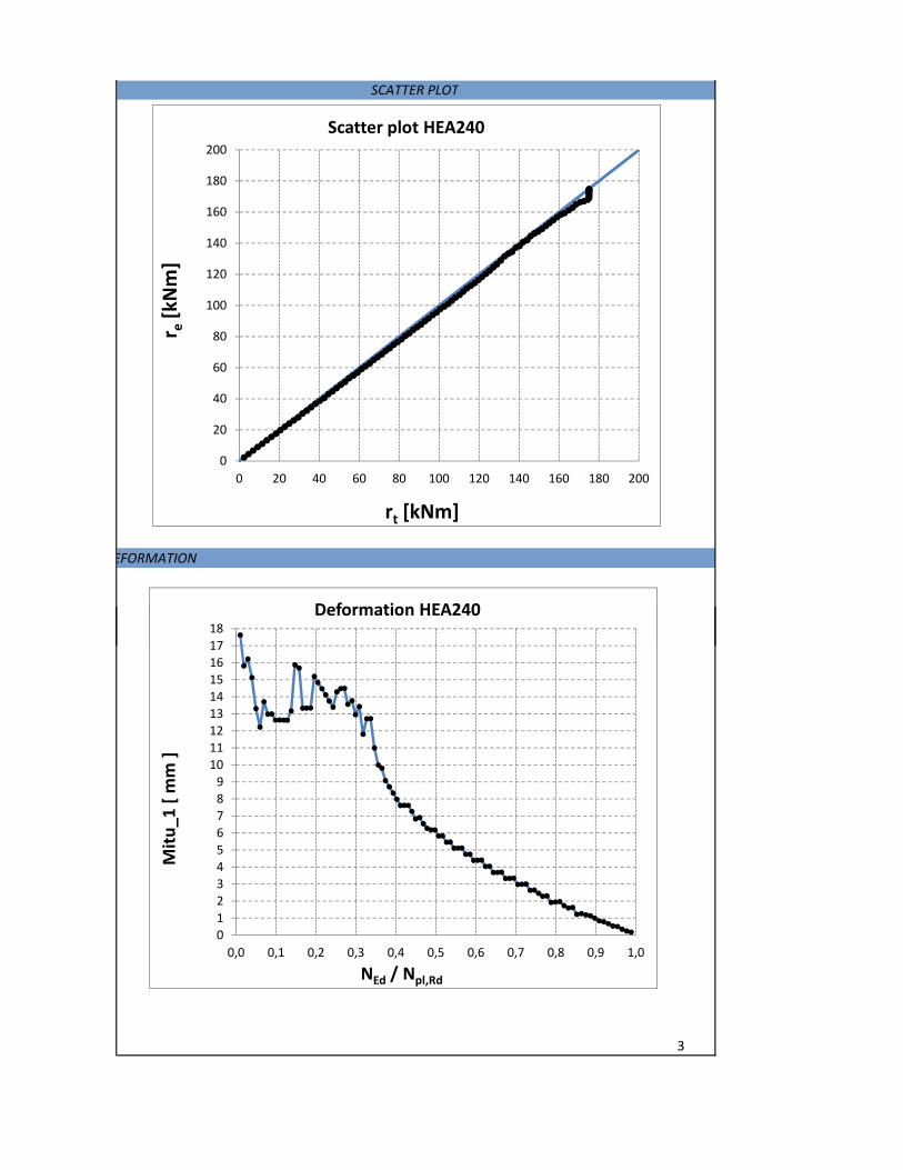
EFORMATION
SCATTER PLOT
0
20
40
60
80
100
120
140
160
180
200
0 20 40 60 80 100 120 140 160 180 200
r e[kNm]
rt [kNm]
Scatter plot HEA240
1718
Deformation HEA240
3
0123456789
101112131415161718
0,0 0,1 0,2 0,3 0,4 0,5 0,6 0,7 0,8 0,9 1,0
Mitu_1
[ m
m ]
NEd / Npl,Rd
Deformation HEA240
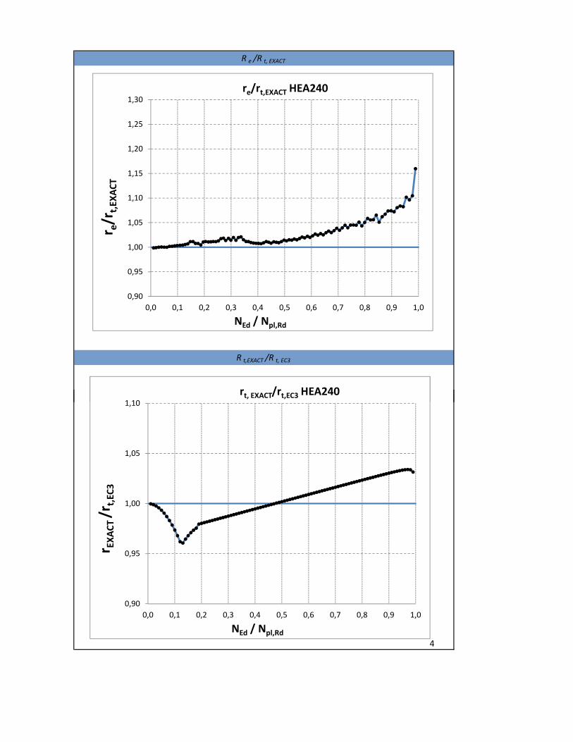
R e /R t, EXACT
R t,EXACT /R t, EC3
0,90
0,95
1,00
1,05
1,10
1,15
1,20
1,25
1,30
0,0 0,1 0,2 0,3 0,4 0,5 0,6 0,7 0,8 0,9 1,0
r e/r
t,EX
ACT
NEd / Npl,Rd
re/rt,EXACT HEA240
1 10rt, EXACT/rt,EC3 HEA240
4
0,90
0,95
1,00
1,05
1,10
0,0 0,1 0,2 0,3 0,4 0,5 0,6 0,7 0,8 0,9 1,0
r EXACT /r
t,EC3
NEd / Npl,Rd
rt, EXACT/rt,EC3 HEA240

0.00 < n < 0.25 26 tests
0.25 ≤ n < 0.50 27 tests
0.50 ≤ n < 0.75 25 tests
0.75 ≤ n < 1.00 21 tests
Total 99 tests
b 0,984
Δbar ‐0,004
sΔ2
0,0001
Vδ 0,0120
γM* 0,989
HEB200
TEST RESULTS
My‐N INTERACTION DIAGRAM
0,8
0,9
1,0
My‐N interaction HEB200
1
0,0
0,1
0,2
0,3
0,4
0,5
0,6
0,7
0,8
0,0 0,1 0,2 0,3 0,4 0,5 0,6 0,7 0,8 0,9 1,0
My,Ed
/ M
pl,y,Rd
NEd / Npl,Rd
Nummerical testsEurocode 3 nominal HEB200Exact solution HEB200

HISTOGRAM
R e /R t,EC3
565860
Histogram HEB200
0,90
0,95
1,00
1,05
1,10
1,15
0,0 0,1 0,2 0,3 0,4 0,5 0,6 0,7 0,8 0,9 1,0
r e/r
t,EC3
NEd / Npl,Rd
re/rt,EC3 HEB200
Nummerical tests
2
024681012141618202224262830323436384042444648505254565860
0,95 1,00 1,05 1,10 1,15
Number of observations
re / rt

DEFORMATION
SCATTER PLOT
0
20
40
60
80
100
120
140
160
180
200
0 20 40 60 80 100 120 140 160 180 200
r e[kNm]
rt [kNm]
Scatter plot HEB200
24
26
Deformation HEB200
3
0
2
4
6
8
10
12
14
16
18
20
22
24
26
0,0 0,1 0,2 0,3 0,4 0,5 0,6 0,7 0,8 0,9 1,0
Mitu_1
[ m
m ]
NEd / Npl,Rd
Deformation HEB200

R e /R t,EXACT
R t,EXACT / R t,EC3
0,90
0,95
1,00
1,05
1,10
1,15
1,20
1,25
1,30
0,0 0,1 0,2 0,3 0,4 0,5 0,6 0,7 0,8 0,9 1,0
r e/r
t,EX
ACT
NEd / Npl,Rd
re/rt,EXACT HEB200
1 10
rt,XACT /rt,EC3 HEB200
4
0,90
0,95
1,00
1,05
1,10
0,0 0,1 0,2 0,3 0,4 0,5 0,6 0,7 0,8 0,9 1,0
r EXACT /r
t,EC3
NEd / Npl,Rd
rt,XACT /rt,EC3 HEB200

0.00 < n < 0.25 25 tests
0.25 ≤ n < 0.50 26 tests
0.50 ≤ n < 0.75 25 tests
0.75 ≤ n < 1.00 23 tests
Total 99 tests
b 0,980
Δbar 0,011
sΔ2
0,0005
Vδ 0,0231
γM* 0,995
TEST RESULTS
My‐N INTERACTION DIAGRAM
IPE330
0,8
0,9
1,0
My‐N interaction IPE330
1
0,0
0,1
0,2
0,3
0,4
0,5
0,6
0,7
0,8
0,0 0,1 0,2 0,3 0,4 0,5 0,6 0,7 0,8 0,9 1,0
My,Ed
/ M
pl,y,Rd
NEd / Npl,Rd
Nummerical testsEurocode 3 nominal IPE330Exact solution IPE330
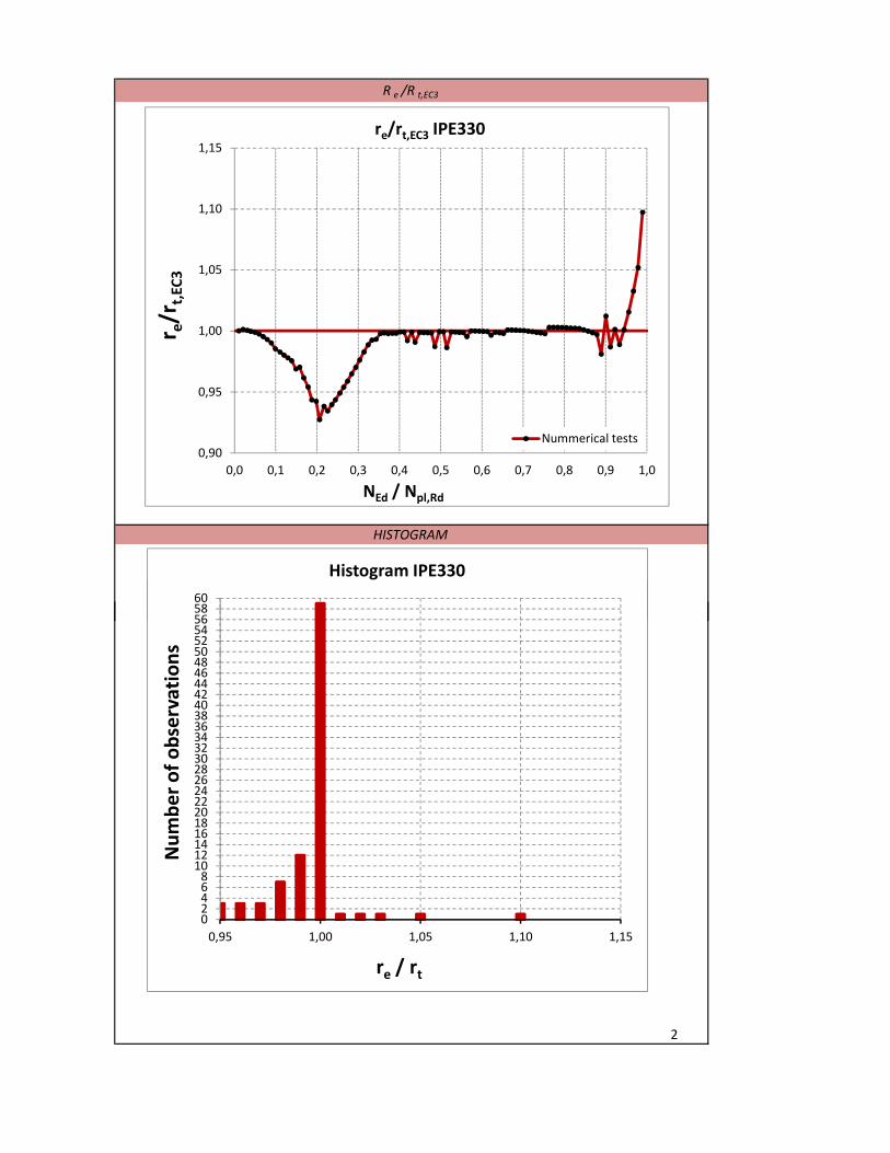
HISTOGRAM
R e /R t,EC3
565860
Histogram IPE330
0,90
0,95
1,00
1,05
1,10
1,15
0,0 0,1 0,2 0,3 0,4 0,5 0,6 0,7 0,8 0,9 1,0
r e/r
t,EC3
NEd / Npl,Rd
re/rt,EC3 IPE330
Nummerical tests
2
024681012141618202224262830323436384042444648505254565860
0,95 1,00 1,05 1,10 1,15
Number of observations
re / rt

DEFORMATION
SCATTER PLOT
0
20
40
60
80
100
120
140
160
180
200
0 20 40 60 80 100 120 140 160 180 200
r e[kNm]
rt [kNm]
Scatter plot IPE330
24
26
Deformation IP330
3
0
2
4
6
8
10
12
14
16
18
20
22
24
26
0,0 0,1 0,2 0,3 0,4 0,5 0,6 0,7 0,8 0,9 1,0
Mitu_1
[ m
m ]
NEd / Npl,Rd
Deformation IP330

R e /R t,EXACT
R t,EXACT /R t,EC3
0,90
0,95
1,00
1,05
1,10
1,15
1,20
1,25
1,30
0,0 0,1 0,2 0,3 0,4 0,5 0,6 0,7 0,8 0,9 1,0
r e/r
t,EX
ACT
NEd / Npl,Rd
re/rt,EXACT IPE330
rt,EXACT /rt,EC3 IPE330
4
0,90
0,95
1,00
1,05
1,10
0,0 0,1 0,2 0,3 0,4 0,5 0,6 0,7 0,8 0,9 1,0
r EXACT /r
t,EC3
NEd / Npl,Rd
rt,EXACT /rt,EC3 IPE330
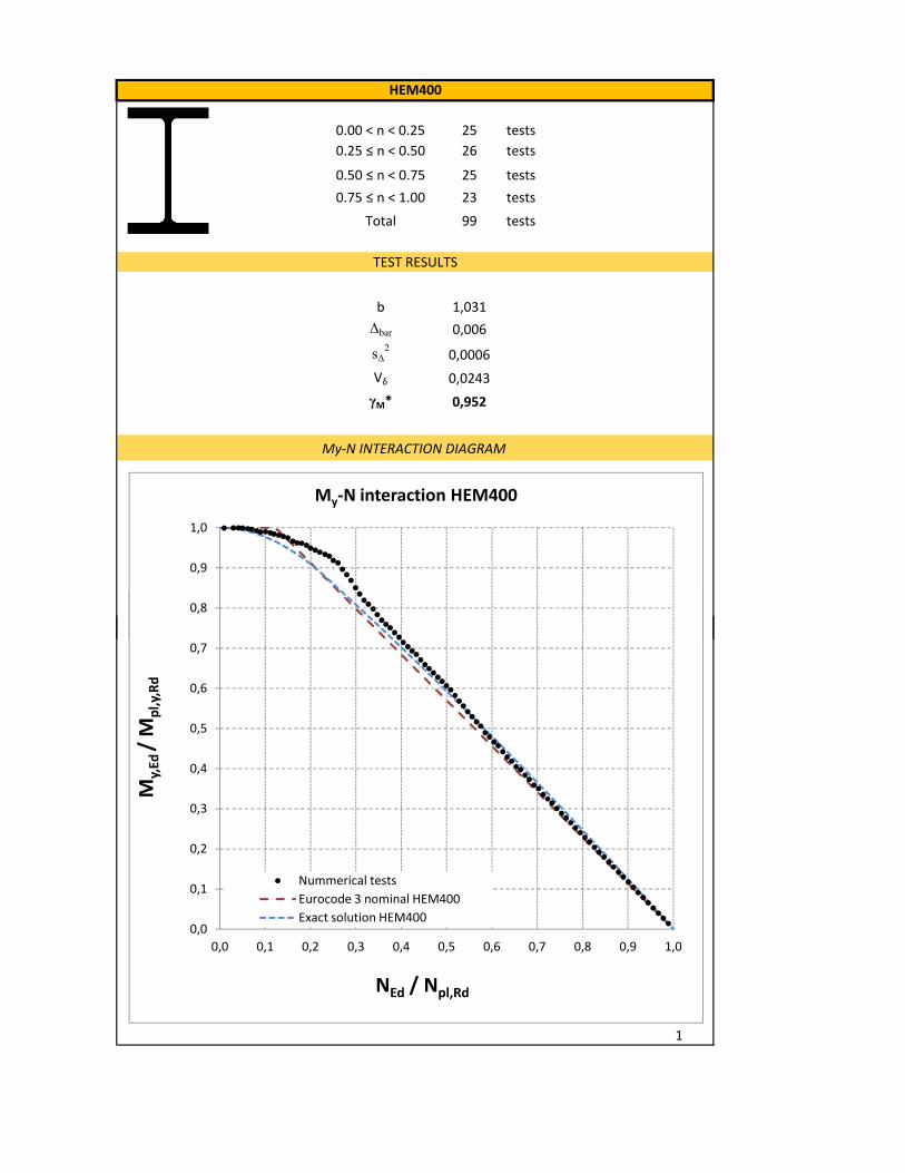
0.00 < n < 0.25 25 tests
0.25 ≤ n < 0.50 26 tests
0.50 ≤ n < 0.75 25 tests
0.75 ≤ n < 1.00 23 tests
Total 99 tests
b 1,031
Δbar 0,006
sΔ2
0,0006
Vδ 0,0243
γM* 0,952
HEM400
TEST RESULTS
My‐N INTERACTION DIAGRAM
0,8
0,9
1,0
My‐N interaction HEM400
1
0,0
0,1
0,2
0,3
0,4
0,5
0,6
0,7
0,8
0,0 0,1 0,2 0,3 0,4 0,5 0,6 0,7 0,8 0,9 1,0
My,Ed
/ M
pl,y,Rd
NEd / Npl,Rd
Nummerical tests
Eurocode 3 nominal HEM400
Exact solution HEM400
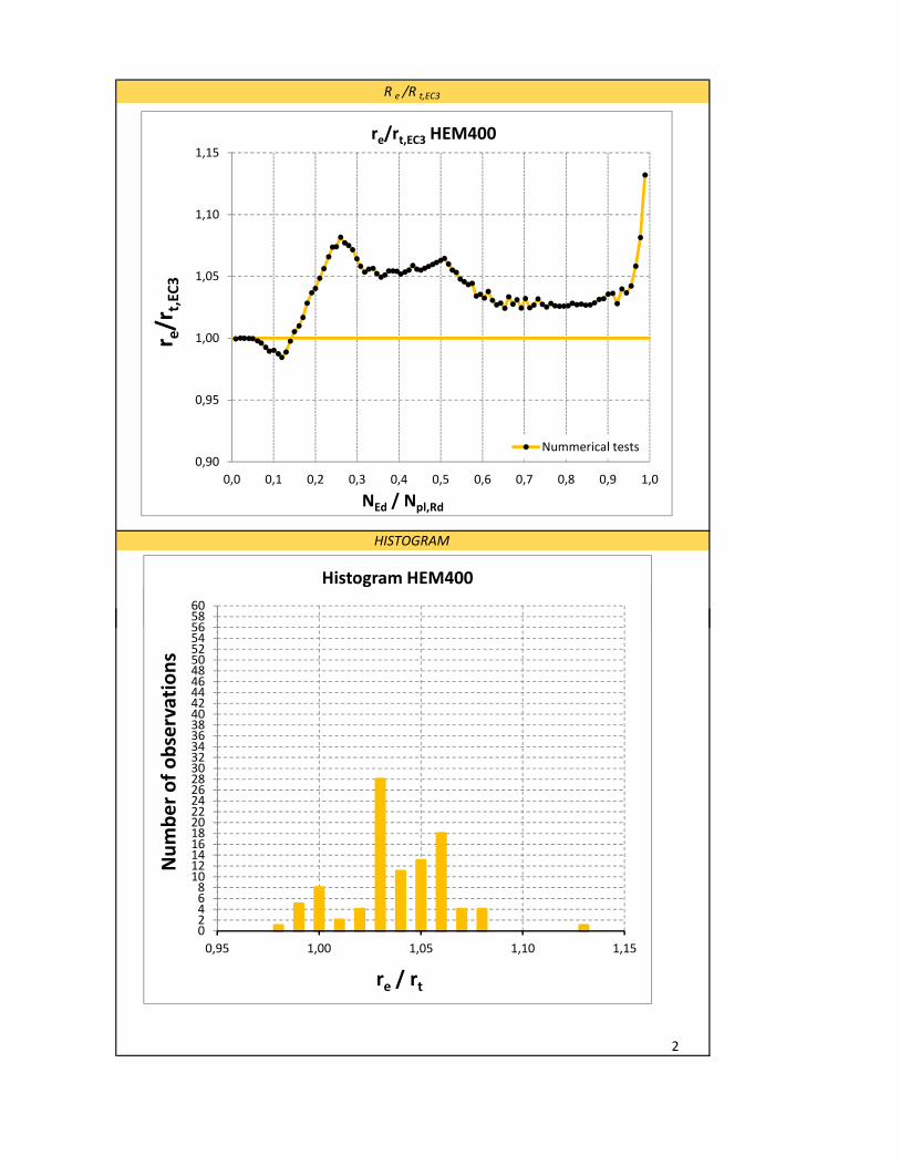
R e /R t,EC3
HISTOGRAM
565860
Histogram HEM400
0,90
0,95
1,00
1,05
1,10
1,15
0,0 0,1 0,2 0,3 0,4 0,5 0,6 0,7 0,8 0,9 1,0
r e/r
t,EC3
NEd / Npl,Rd
re/rt,EC3 HEM400
Nummerical tests
2
024681012141618202224262830323436384042444648505254565860
0,95 1,00 1,05 1,10 1,15
Number of observations
re / rt

DEFORMATION
SCATTER PLOT
0
200
400
600
800
1000
1200
1400
0 200 400 600 800 1000 1200 1400
r e[kNm]
rt [kNm]
Scatter plot HEM400
384042
Deformation HEM400
3
024681012141618202224262830323436384042
0,0 0,1 0,2 0,3 0,4 0,5 0,6 0,7 0,8 0,9 1,0
Mitu_1
[ m
m ]
NEd / Npl,Rd
Deformation HEM400

R e /R t,EXACT
R t,EXACT /R t,EC3
0,90
0,95
1,00
1,05
1,10
1,15
1,20
1,25
1,30
0,0 0,1 0,2 0,3 0,4 0,5 0,6 0,7 0,8 0,9 1,0
r e/r
t,EX
ACT
NEd / Npl,Rd
re/rt,EXACT HEM400
1 10
rt,EXACT /rt,EC3 HEM400
4
0,90
0,95
1,00
1,05
1,10
0,0 0,1 0,2 0,3 0,4 0,5 0,6 0,7 0,8 0,9 1,0
r EXACT /r
t,EC3
NEd / Npl,Rd
rt,EXACT /rt,EC3 HEM400

0.00 < n < 0.25 101 tests
0.25 ≤ n < 0.50 106 tests
0.50 ≤ n < 0.75 100 tests
0.75 ≤ n < 1.00 89 tests
Total 396 tests
b 1,028
Δbar ‐0,032
sΔ2
0,0009
Vδ 0,0306
γM* 0,962
TEST RESULTS
My‐N INTERACTION DIAGRAM
TOTAL
0,8
0,9
1,0
My‐N interaction all cross‐sections
HEA240
HEB200
IPE330
HEM400
1
0,0
0,1
0,2
0,3
0,4
0,5
0,6
0,7
0,8
0,0 0,1 0,2 0,3 0,4 0,5 0,6 0,7 0,8 0,9 1,0
My,Ed
/ M
pl,y,Rd
NEd / Npl,Rd
HEM400
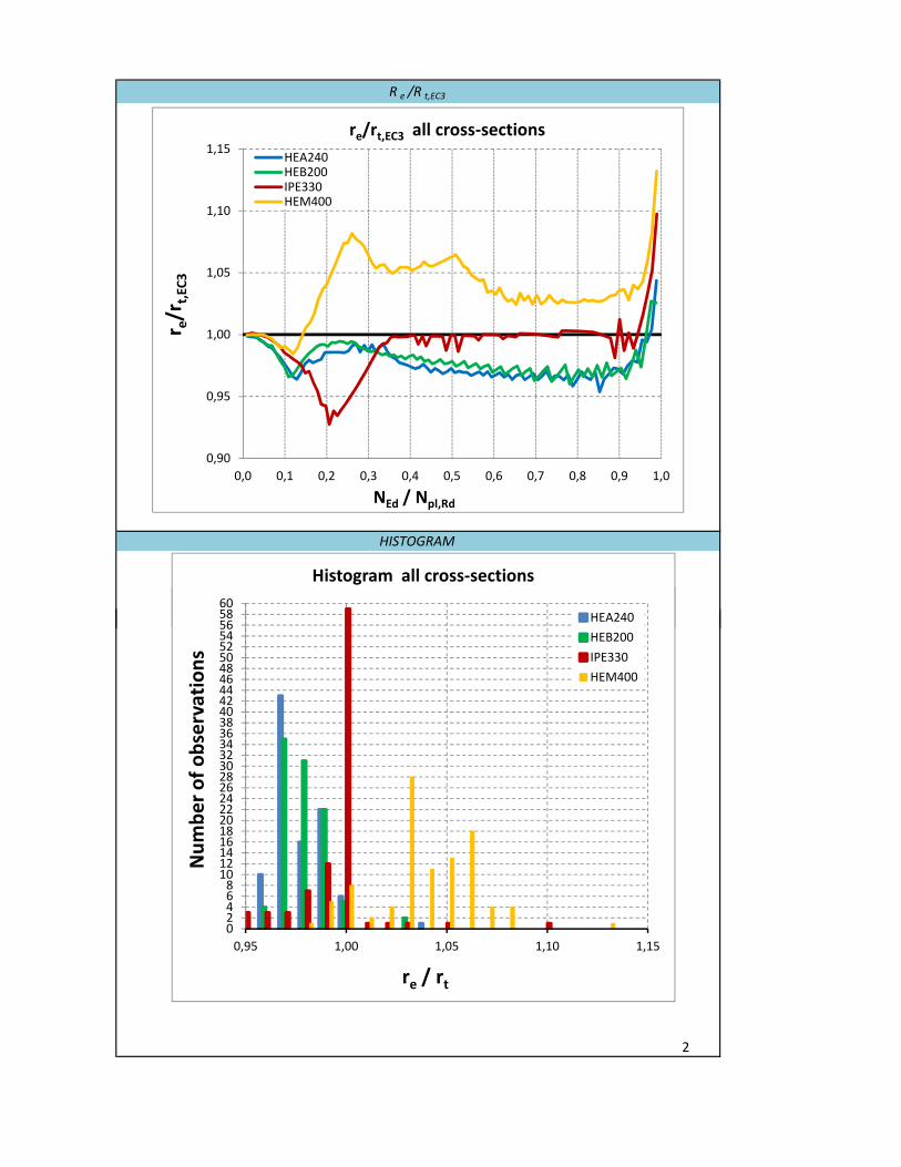
HISTOGRAM
R e /R t,EC3
565860
Histogram all cross‐sections
HEA240
0,90
0,95
1,00
1,05
1,10
1,15
0,0 0,1 0,2 0,3 0,4 0,5 0,6 0,7 0,8 0,9 1,0
r e/r
t,EC3
NEd / Npl,Rd
re/rt,EC3 all cross‐sections
HEA240HEB200IPE330HEM400
2
024681012141618202224262830323436384042444648505254565860
0,95 1,00 1,05 1,10 1,15
Number of observations
re / rt
HEA240
HEB200
IPE330
HEM400

0.00 < n < 0.25 b 1,011 S235 b 1,028
Δbar ‐0,022 Δbar ‐0,032
sΔ2 0,0006 sΔ
2 0,0009
Vδ 0,0255 Vδ 0,0306
γM* 0,976 γM* 0,962
0.25 ≤ n < 0.50 b 1,056 S355 b 1,028
Δbar ‐0,042 Δbar ‐0,032
sΔ2 0,0019 sΔ
2 0,0009
Vδ 0,0436 Vδ 0,0306
γM* 0,959 γM* 0,999
0.50 ≤ n < 0.75 b 1,038 S460 b 1,028
Δbar ‐0,044 Δbar ‐0,032
sΔ2
0,0006 sΔ2
0,0009
Vδ 0,0255 Vδ 0,031
γM* 0,946 γM* 1,049
0.75 ≤ n < 1.00 b 1,026
Δbar ‐0,025
sΔ2 0,0011
Vδ 0,0331
γM* 0 967
STEEL GRADESUBSET N
γM 0,967
0.10 ≤ n < 0.15 b 0,973
Δbar 0,000
sΔ2 0,0000
Vδ 0,0062
γM* 0,999